1. Introduction
About 99% of the electromagnetic energy emitted by the Earth’s atmosphere system is distributed in the spectral range of 3–80 µm [
1]. The water vapour, which strongly absorbs the radiation in this band [
2,
3,
4,
5], turns out to be an important component for the atmospheric radiative processes and hence for the evolution of the Earth’s climate. According to Lacis et al. [
6], the water vapour is responsible for 75% of the greenhouse effect. This results in a warming increase, which leads to greater evaporation and a consequent increase in cloud formation and precipitation levels.
The water vapour was included in the list of Essential Climate Variables (ECV), contributing to the characterization of Earth’s climate according to the definition given by the Global Climate Observing System (GCOS). GCOS assesses the status of the global climate observations needed to support climate research and services.
Polar regions are areas of the Earth that play a key role in the global climate system through the interaction with the oceans, atmosphere, and ecosystems. In the last two decades, the Arctic surface air temperature has increased by more than twice the global average [
7]. Moreover, there are signals of further Arctic warming [
8], even if the mechanisms for Arctic amplification are still under discussion [
9].
Unlike the Arctic, the Antarctic continent has shown less uniform temperature changes during the past 30–50 years, with the warming of West Antarctica and no significant overall change in East Antarctica [
10,
11]. However, these results are preliminary owing to the few in situ sensors to detect the water vapour. Furthermore, due to the logistics, large areas of these regions cannot be covered by sensors placed in situ. Considering the importance of the polar regions in the Earth’s climate system, we carried out a study using the available data from the last 20 years collected by the in-situ sensors (GNSS and Radiosonde). Moreover, we made use of values in the same areas from the reanalysis model ERA-Interim [
12].
The study is focused on the moisture content changes in the atmospheric column. In the last decades, the water vapour content in the atmosphere has been the subject of several studies, which have adopted various techniques for its quantitative assessment.
By definition, the “Total column of water vapour” is the total amount of water vapour in the vertical column of air extending from the surface of the ground to the top of the atmosphere. This is also called “Integrated Water Vapour” (IWV) or “Precipitable Water Vapour” (PWV or PW) since the water vapour could potentially precipitate. In this work, the PW (in mm) is the main observable.
The principal objective of this work was to provide reliable trend of the PW long time series in the Polar regions. Together with updated results for RS and GNSS stations already analysed in previous studies, we present new results for most recently installed stations in West Antarctica. All the data were processed with a homogeneous, coherent, and up-to-date processing strategy, in order to minimize the problems and the limits of the different techniques used.
The PW varies both in space and time [
13,
14,
15] and its measurement is challenging. Several techniques are currently used to derive the PW such as ground-based instrumentation from GNSS, in-situ measurements from RS, and sensors on board satellites. Several studies have been carried out to compare the retrievals from different techniques, observations, and re-analyses. An overview and comparison of different PW measurement techniques are given in Guerova et al. [
16], Parracho et al. [
17], Van Malderen et al. [
18], Triana-Gomez et al. [
19]. These studies focused on the optimization of the data processing to produce time series free from non-climatic effects and, consequently, obtain reliable climate signals. Van Malderen et al. [
20] carried out a detailed assessment of break detection methods to obtain homogeneous GPS IWV time series. Furthermore, the entire available GNSS dataset was reprocessed to take into account the updated reference frame, new models, different mapping functions, and different processing strategies [
21,
22,
23,
24,
25].
The most important advantage of using GNSS is that it works under all weather conditions with high precision, great temporal and potentially, spatial resolution at relatively low cost. Daily GPS time series have been available since the mid-90s, however, reprocessing of all this bulk of data requires either additional weather parameters from meteorological stations or reanalysis products, as from a numerical weather prediction model reanalysis (ERA-Interim).
Estimating PW trends in some areas of the Earth has often shown great uncertainty, e.g., analysing five different re-analyses Dessler and Davis [
26] found that the uncertainties in long-term trends needed to be reduced before using them for climate interpretations. Schroeder et al. [
27] also found problems in estimating trends from satellite data. Due to different types of uncertainties, GPS often is used for validation. Recently, detailed studies attempting to derive accurate GNSS PWV values were carried out by Ssenyunzi et al. [
28] in the East African tropical region, in which they assessed whether reanalysis data can substitute surface meteorological data if absent.
Studies carried out by Tomasi et al. [
29] on RS and Rinke et al. [
30] using RS, reanalysis models, and GPS data reported PW trends characterising the evolution of the water vapour in the Arctic atmosphere.
PWV trends can also be derived from ground-based microwave radiometers (MW) and Fourier transform infrared (FTIR) spectrometers; trends from these instruments have been compared with estimates from GNSS in Bernet et al. [
31] showing that GNSS data homogeneously reprocessed can be trusted to calculate climatic PWV trends. Moreover, Virolainen et al. [
32] compared the PWV estimates obtained from FTIR, MW, and GPS techniques and found a good agreement between them.
The variability of the PW is a very important issue for the study of climate change and the assessment of long-term trends in water vapour is crucial. To this end, it is necessary to assess the statistical significance of each estimated PW trend, which depends on its magnitude, the autocorrelation in time series, and its length in time [
14]. The authors assessed that the time it takes to detect significant PW trends ranges from 28 to 40 years. However, only sparse GPS stations will reach the lower limit in the next few years. Anyway, it has been shown that a full exploitation of available GPS time series is important, e.g., for the validation of water vapour estimation from radiosonde and satellite data [
33,
34], or assimilation into numerical weather models (Bennitt and Jupp [
35] and references therein). GNSS demonstrated its ability to make great contribution in the retrieval of the water vapour content in remote areas as well.
The present study investigates the assessment of the accuracy of PW retrieval, from GNSS and RS techniques, in particular in Arctic and Antarctic regions, where data are still scarce and often not easy to collect. At the same time, we explore the capability of the old and new permanent GNSS stations installed in Arctic and Antarctic regions to provide reliable estimates of precipitable water vapour (PW). To achieve this goal, PWGPS were compared with PWRS and with the ERA-Interim reanalysis model. Once validated, data were used for estimating long-term trends in Arctic and Antarctic regions. A discussion of these findings was held to consider the impact of the atmospheric water vapour content on weather and climate.
This paper is organized as follows.
Section 2 describes the characteristics and processing of the observations collected in polar regions using GNSS systems and radiosondes.
Section 3 deals with long time series of PW retrieved from GNSS and RS, their cross-validation and comparison with the ERA-Interim model.
Section 4 investigates different noise models and trend estimations from long time series of PW are carried out and discussed. In
Section 5, some conclusions are drawn.
2. Methodology and Data Collection in Polar Regions
The main purpose of this work was to produce long time series of PW, retrieved at the GNSS and RS co-located sites, for cross-validation and testing of appropriate methods, with the aim to provide new results of Earth’s polar regions. For those sites where RS instrumentation is not available, we processed only GNSS data (from old and new sites).
2.1. GNSS Data Selection and Processing for PW Retrieval
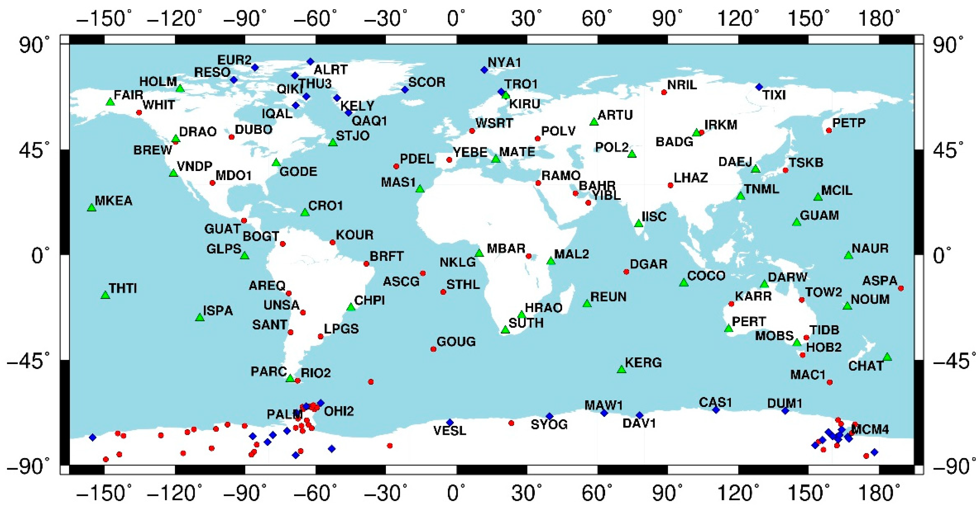
In this study, daily observation data of 208 GNSS stations distributed worldwide for over 20 years were processed. Stations belong to different GNSS networks, including the International GNSS Service (IGS) network, the Victoria Land Network for DEFormation control (VLNDEF), and the Polar Earth Observing Network (POLENET). More details about this dataset and its accurate identification and selection are given in Zanutta et al. [
36].
It is worth mentioning that during the polar year 2007–2008, a large effort was made by UNAVCO to install a series of GNSS stations in West Antarctica. At present, more than 100 GNSS stations operate in Antarctica, most of which are permanent stations and have been collecting data for more than 10 years.
Among the selected 208 GNSS stations, a global network of 38 permanent IGS stations was included during GPS data processing to frame the results in the International Terrestrial Reference Frame ITRF2014 [
37]; see
Figure 1.
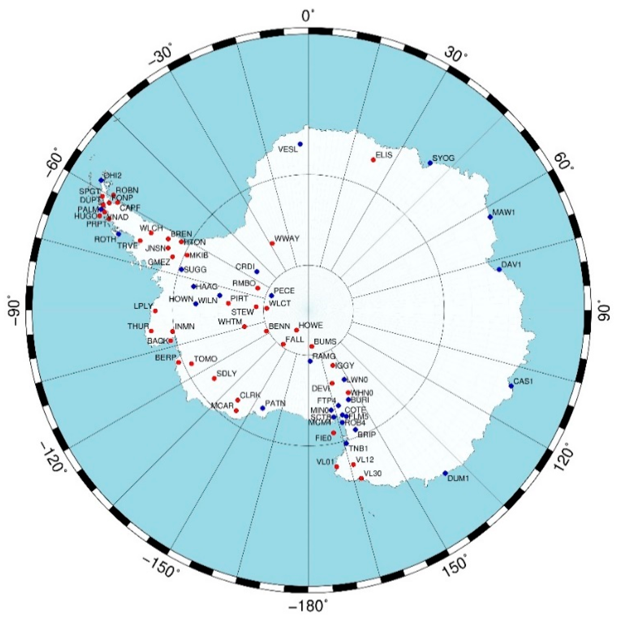
We selected 13 GNSS stations in the Arctic regions, close to radiosonde stations that make use of Vaisala sensors. In Antarctica, most of the available permanent stations were analysed (
Figure 2), and 27 were selected for the required characteristics (see below).
The GPS data were processed using the Bernese Processing Engine (BPE), a tool of the Bernese GNSS software v5.2 [
38]. Bernese is scientific, high-precision, multi-GNSS data processing software. It features state-of-the-art modeling and up-to-date standards adopted internationally. Furthermore, it allows you to set all relevant processing options and BPE is a powerful automation tool when processing huge amounts of data. Carrier-phase double difference approach was used to process the daily observation files, together with a sampling rate of 30 s and an elevation cutoff angle of 10°.
From the IGS repro2 campaign (
https://cddis.nasa.gov/archive/gps/products/repro2, last visit on 26 November 2021) and official IGS solutions, the following products were used: IGS station coordinates, satellite orbits and Earth Orientation Parameters (EOP), antenna phase centre offsets (PCOs) and variations (PCVs) (both for satellite and receiver antennas). Corrections and models in IERS2013 Conventions were applied.
For Zenith Total Delay (ZTD) computation, the hydrostatic and wet Vienna Mapping Functions (VMF1; [
39]) were used. A very crucial point in analysing data at high latitudes is the a priori Zenith Hydrostatic Delay (ZHD) in order to obtain a more reliable Zenith Wet Delay (ZWD). With this aim, the Bernese software was modified accordingly by adding the Global Pressure and Temperature 2 (GPT2w) model [
40], allowing these much more reliable results in the coordinate computation and consequently in the ZWD estimation. Further details on the strategy, models, and parameterization adopted during the GPS data processing can be found in
Section 3.1 and
Table 2 of Zanutta et al. [
36].
Although the GPS data were processed with the purpose of ensuring the utmost accuracy of the time series adopting homogeneous, consistent, and up-to-date processing strategies, suited to polar regions, some open issues still remain. Certainly, increasing the number of processed stations would help in network adjustment. The use of more refined atmospheric models and products, such as VMF3 [
41], could allow us to observe at lower elevations and better decouple estimated height and ZTD at stations. For some sites, especially in the inner Antarctic region, negative ZWD values were retrieved, suggesting that the ZHD model should be improved or that the data analysis needs to be further refined (see
Section 3 and
Section 4). Indeed, very small ZWD values are sought, at the limit of the accuracy of the GPS technique.
The PW was retrieved from GPS data using the mean temperature of the atmosphere (T
m) obtained integrating radiosonde profiles: more details are given in
Section 2.2 and in Negusini et al. [
24].
Metadata of the GPS stations adopted in this study, both in the Arctic and Antarctic regions for PW retrieval are listed in
Table 1 and
Table 2, respectively. As a general criterion, stations with data spanning less than 10 years were excluded from the PW retrieval studies, except for some stations that are important for GPS—RS comparison, such as IQAL and ROTH.
2.2. Radio Sounding Data Selection and Processing for PW Retrieval
For the purposes of the present study, 16 RS stations were selected, i.e., stations where radiosondes lunches are co-located with GNSS sites. Among these, 6 sites are in Antarctica: Casey, Davis, Mawson, McMurdo, Mario Zucchelli, and Rothera. The remaining 10 sites are in the Arctic: Alert, Eureka, Iqaluit, Aasiat, Andoya, Ny Alesund, Narsarsquaq, Resolute, Ittoqqpprtmiit, and Tiksi. The raw data recorded at these stations were downloaded from the World Meteorological Organization (WMO) database of the University of Wyoming), except for data recorded at the Mario Zucchelli station, collected by the Italian Meteo-Climatological Observatory and Rothera provided by the British Antarctic Survey (NCAS British Atmospheric Data Centre).
The dataset analysed was collected from 1998 to 2017 through more than 122.000 RS launches of Vaisala radiosondes (models RS-80, RS-90, and RS-92). Other radiosonde models like BAR, MRZ, and Marz2-2 were the most frequently used at the site of Tiksi [
41]. Each radiosonde measurement provides the values of the atmosphere pressure p (hPa), temperature T (°C), and relative humidity RH (%). These values are registered at different altitudes z, with a resolution that usually changes between 5 and 50 m depending on the ground recording equipment. The radiosonde measurements are affected by various external and internal factors that introduce errors to different extent of importance. RS measurements have been studied by many authors, e.g., Turner et al. [
43], Wang et al. [
44], Mattioli et al. [
45], and Ho et al. [
46], which highlighted the presence of different errors. In order to correct these errors, several methods based on the analysis of data provided by different Vaisala radiosonde models were proposed in the past two decades (e.g., [
47,
48,
49,
50]). The pressure error of Vaisala radiosondes usually does not exceed 0.5 hPa, a value for which it is assumed that no specific correction is required [
24]. On the contrary, temperature and RH measurements require specific corrections to obtain reliable results, especially for the latter. A procedure that groups together most of the correction methods for the Vaisala radiosondes was developed by Tomasi et al. [
51,
52]. Discussion on the errors and different approaches to correct BAR, MRZ, and Marz2-2 radiosonde observations can be found in Tomasi et al. [
29].
To validate the column water vapour content retrieved from the GPS signal, the precipitable water from the radiosonde data PW
RS was determined together with the mean temperature T
m. Both PW
RS and T
m were estimated according to the procedure described in Negusini et al. [
24]. Briefly, the tropospheric water vapour content was calculated for each RS measurement through the integration of the vertical distribution curve of the absolute humidity
q(
z) from the surface-level to 12 km altitude. The
q(
z) value was calculated using the vertical profiles of
T(
z) and
RH(
z) appropriately corrected for the main lag, instrumental errors, and the various dry biases:
where
Rw is the water vapour gas constant. The water vapour partial pressure
e(
z), measured in hPa is given at each level by the product
RH(
z) ×
E(
T(
z)), where the
E(
T(
z)) value is the saturated water vapour pressure in the pure phase over a plane surface of pure liquid water, which was calculated by using the formula of Murphy and Koop [
53]. The total PW
RS is obtained by adding to the integrated value of
q(
z) the monthly average values of stratospheric water vapour content (
z > 12 km) derived from the observations carried out using the Michaelson Interferometer for Passive Atmospheric Sounding (MIPAS)–Environmental Satellite (ENVISAT) [
51]. The contribution of the stratosphere humidity to the column PW is between 4 × 10
−3 and 6 × 10
−3 mm, which is much below the tropospheric PW levels. However, during the austral winter, PW in Antarctica could decrease appreciably below 1 mm, as shown in the following section, and in these cases, the weight of the stratospheric precipitable water can range from 1% to 6%.
Parameter
Tm is the average value of the air temperature, calculated on the vertical atmospheric path by using the vertical profile of
e(
z) as a weight function as follows:
Equation (2) represents the ratio of the integrals determined in the altitude range from the surface level z0 to zTR = 12 km; the vertical profiles of e(z) and T(z) were derived from RS measurements. Considering that parameter e(z) is used as a weight function in both integrals, the parameter Tm can be defined as the average tropospheric temperature, which is calculated as the sum of the contributions given by the various atmospheric layers weighted on the basis of their moisture characteristics.
The RS stations located in the Arctic and Antarctica are listed in
Table 3 and
Table 4 along with their main characteristics.
According to the general criterion of selecting data, Andoya’s RS site is not taken into account because its time interval is too short (only 1.5 year). The Aasiat and Narsarsquaq data are anyway used in further analysis even if their data availability is just under 10 years. Finally, Rothera data were processed but not used for long-term trend estimation, due to the short time interval of the available data.
3. GPS and RS PW Long Time Series: Cross-Validation and Comparison with ERA
3.1. PW from GPS and RS Long Time Series
For the entire dataset presented in
Section 2.1 and in
Figure 1, only the GPS constellation data over a 20-year span were processed using the Bernese GNSS software.
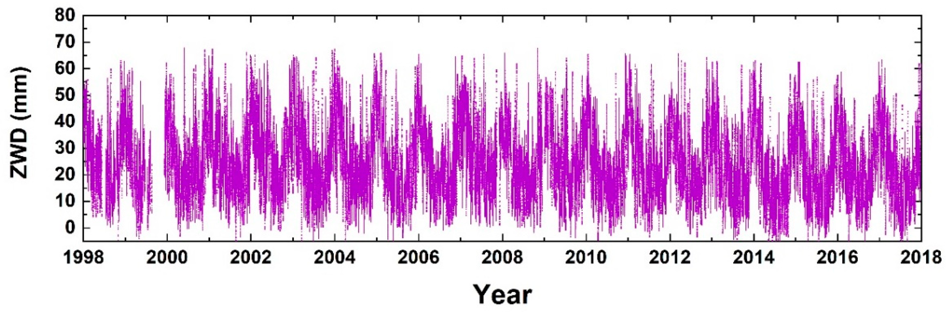
The ZWD parameters were estimated on an hourly basis during the GPS processing. An example of the ZWD time series is shown in
Figure 3.
The annual signal is clearly identified in the time series and more evident in the Arctic, with maximum values ranging from 9 to 17 cm, depending on the latitude of the station; higher latitudes correspond to lower ZWD values. In Antarctica, the maximum values range from 2 to 10 cm, depending on the height of the station (higher altitudes correspond to lower ZWD) and the region to which the station belongs. Higher values are registered in the Antarctic Peninsula, lower values in inland regions, and in coastal stations, the maximum value found was 5 cm.
In order to retrieve PW
GPS (in mm) from ZWD
GPS the well known relation [
54] was used:
The dimensionless factor
Π is given by
where
ρ (in kg·m
−3) is the density of liquid water,
Rw the specific gas constant for water vapour.
k3 is one of the 3 constants
k1,
k2, and
k3 that appear in the formula for atmospheric refractivity
N at radio frequencies [
55].
k’2 can be calculated as
k’2 = k2−mk1, considering that
m=
Mw/
Md is the ratio between the molar masses of water vapour and dry air. Values of
Tm (K) were computed using RS data.
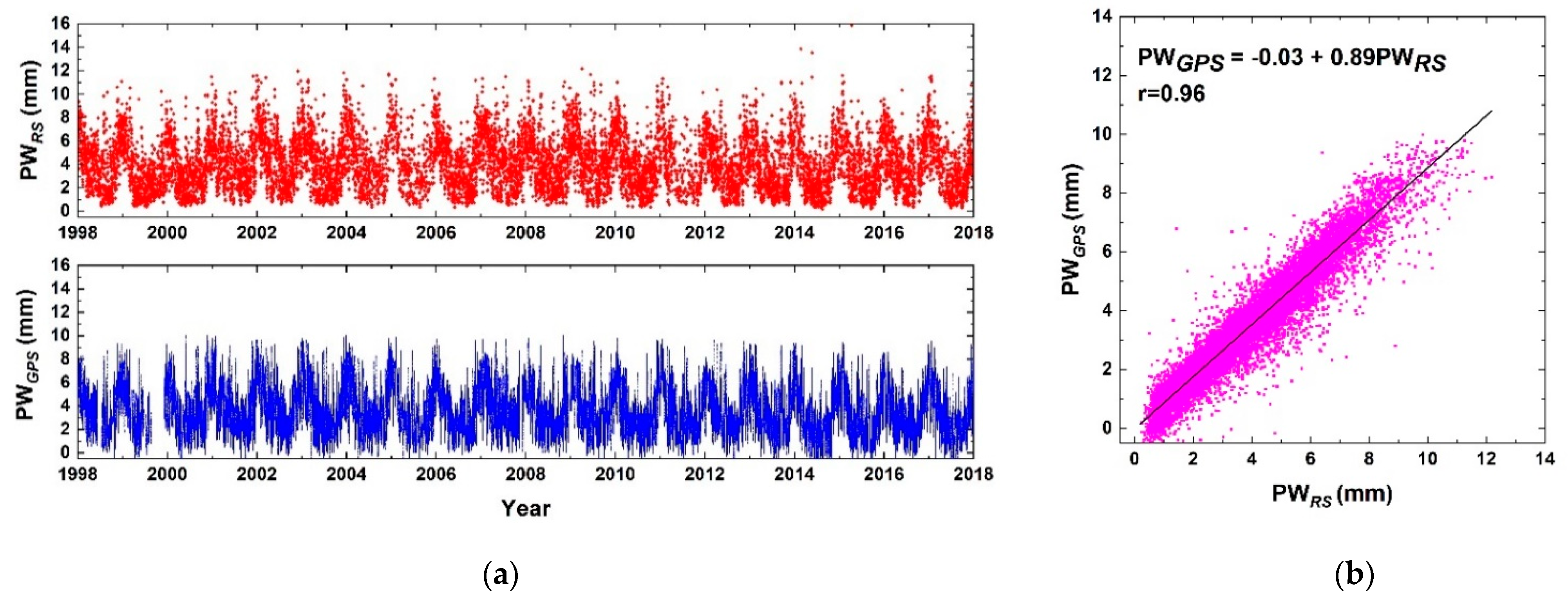
PW estimates for the Casey station obtained from RS (see
Figure 4 left-top) and from GPS (
Figure 4 left-bottom) are displayed during the twenty years. The time series shows a very similar behaviour in terms of seasonal signals, although the RS time series is noisier and presents some higher values of PW. A scatter plot of the two Casey’s PW time series (from GPS and RS) was produced as well, see
Figure 4 (right). There is a very good agreement between the two time series in terms of intercept, slope of the regression line, and correlation coefficient (Pearson’s r = 0.96). Similar behaviours were obtained for all the co-located stations and their results are shown in the following sections.
Most GNSS stations do not have RS instrumentation nearby. When available, often, the time series of PW from RS are shorter than the GPS time series. Therefore, to convert ZWDGPS to PWGPS, another method had to be used, since PWGPS could suffer from the lack of Tm from RS to fully exploit the results.
Bevis et al. [
56] proposed a relation between
Tm and T
s, where T
s is the surface temperature at the investigated station. However, as most GNSS stations do not have co-located weather stations, other methods had to be found to obtain T
s. One method makes use of atmospheric reanalysis models as, e.g., ERA-Interim, which is computed by the European Centre for Medium-Range Weather Forecasts (ECMWF), see Dee et al. [
12].
Another option makes use of the Tm grid values provided by the Wien University of Technology (TU Wien). To estimate the Tm values at the GNSS stations (TmG, hereafter), gridded values were estimated every 6 h using bilinear interpolation.
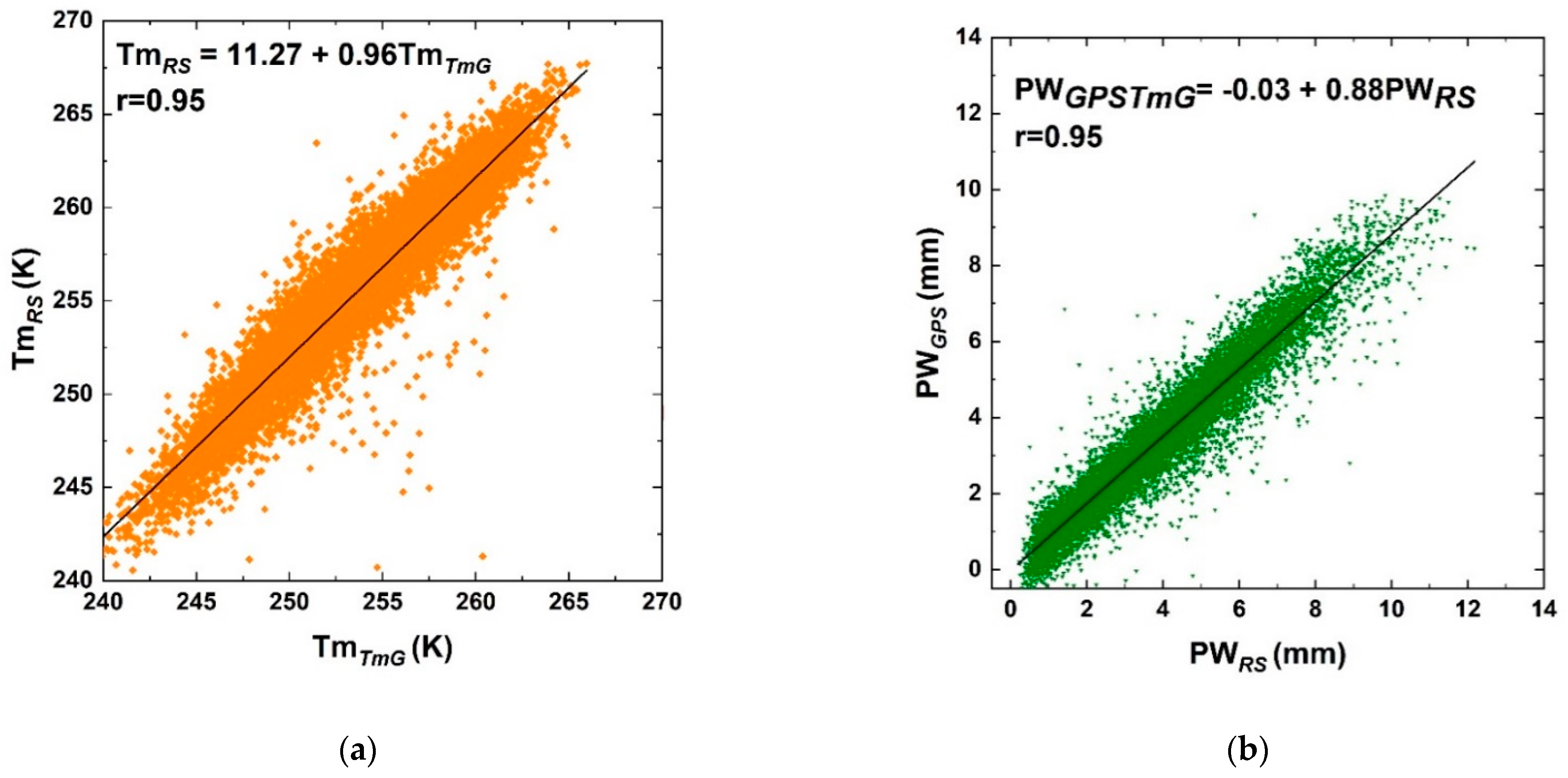
At GPS—RS co-located stations, the two quantities
Tm derived by RS (T
mRS, hereafter) and T
mG were compared. A scatter plot between T
mRS and T
mG, shown in
Figure 5, presents a good agreement, even if it is not possible to state that the two quantities are equal (see
Figure 5a).
The scatter plot between computed PW
GPSTmG (i.e., PW
GPS obtained using T
mG) and PW
RS is shown in
Figure 5b. Taking into account the error range, not shown in
Figure 5a, slope, intercept and Pearson’s correlation coefficient are almost the same as in
Figure 4b. This behaviour was verified for all the co-located stations. For these reasons, the PW
GPS is estimated using the
Tm values from TU Wien, i.e., T
mG, and named PW
GPS, although it would be more correct to call it PW
GPSTmG.
3.2. PW Time Series from ERA-Interim Dataset
In order to have an additional dataset to be compared with the GPS and RS PW time series, ERA-Interim parameters were computed. This dataset is particularly useful for GNSS stations where no sounding data from weather stations are available.
The ERA-Interim is a global atmospheric reanalysis dataset computed by the ECMWF. It covers the interval from 1 January 1979 to 31 August 2019, with a native Gaussian grid spacing of 0.75 × 0.75 degrees, 60 vertical levels, and a temporal resolution of 6 h (0, 6, 12, 18 UTC). The data assimilation system used to produce the ERA-Interim is based on the 2006 release of the Integrated Forecast System (IFS-Cy31r2). This system includes a 4-dimensional variational analysis (4D-Var) with a 12-h analysis window [
57]. An extensive list of all the available parameters can be found in Dee et al. [
12]. Among them, only three sets of parameters were extracted for this study: geopotential height Z (m), specific humidity Q (gKg
−1), and absolute temperature T (K). They were used as input of Ray-traced Delays in the Atmosphere (RADIATE) software to calculate ZWD and ZHD. RADIATE is developed and maintained by TU Wien. It is a ray-tracing software used for geodetic applications and it is freely available. Taking the above three parameters (Z, Q, and T) as input on 25 pressure levels and with a spatial resolution of 1 × 1 degrees, the software can compute several tropospheric ray-traced parameters [
57]. Since this work is focused on precipitable water vapour trend estimations, among all the outputs computed by RADIATE, mainly ZTD, ZHD, and ZWD values at the location of the considered GNSS stations were analysed, even if surface temperature and pressure were obtained. From ZWD obtained by ERA-Interim (ERA, hereafter), and using T
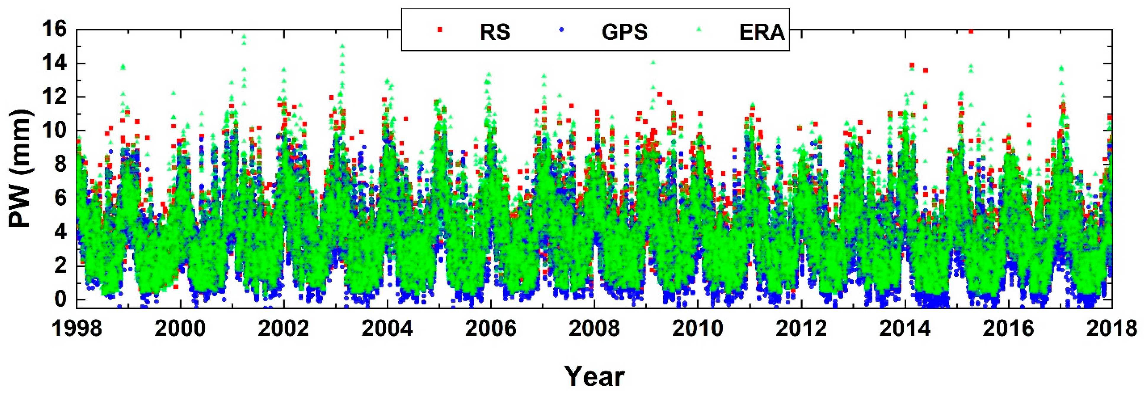
mG values, the PW time series was also calculated for all the GPS stations considered in this study. As an example, the three PW time series are shown in
Figure 6 for the CAS1 station.
It appears that the PW values obtained from ERA are drier than the PW values from the GPS. This kind of statement will be discussed in the next section for all the co-located stations.
3.3. RS PW Comparison with GPS and with ERA (at GPS—RS Co-Located Sites)
Scatter plots of PW values (RS vs. GPS and RS vs. ERA) were produced for all the 14 stations, 9 in the Arctic, and 5 in Antarctica. As explained in
Section 2.2, in Antarctica only 5 out of 6 stations are available, since Rothera (ROTH) was excluded from long-term trend estimation due to the short measurement period available.
For each scatter plot, 6 parameters were estimated:
Bias = mean value of the differences PW_(RS−GPS) and PW_(RS−ERA) (in mm);
RMSD = Root-Mean-Square Deviation of the series of the differences (in mm);
Intercept of the linear regression (in mm);
Slope of the linear regression of the scatter plot;
Pearson’s correlation coefficient;
RMSE = Root-Mean-Square of the Error or residual standard deviation (in mm) that indicates the quality of the fit.
From that point on, the 4-character GNSS code will also be used for RS sites. As a general comment, there is better agreement between PW values from RS and PW values from ERA. This likely depends on RS data assimilation in ERA reanalysis, while GPS is largely model independent, even if some of the products derived from the ECMWF reanalysis models are used within GPS processing and post-processing data analysis.
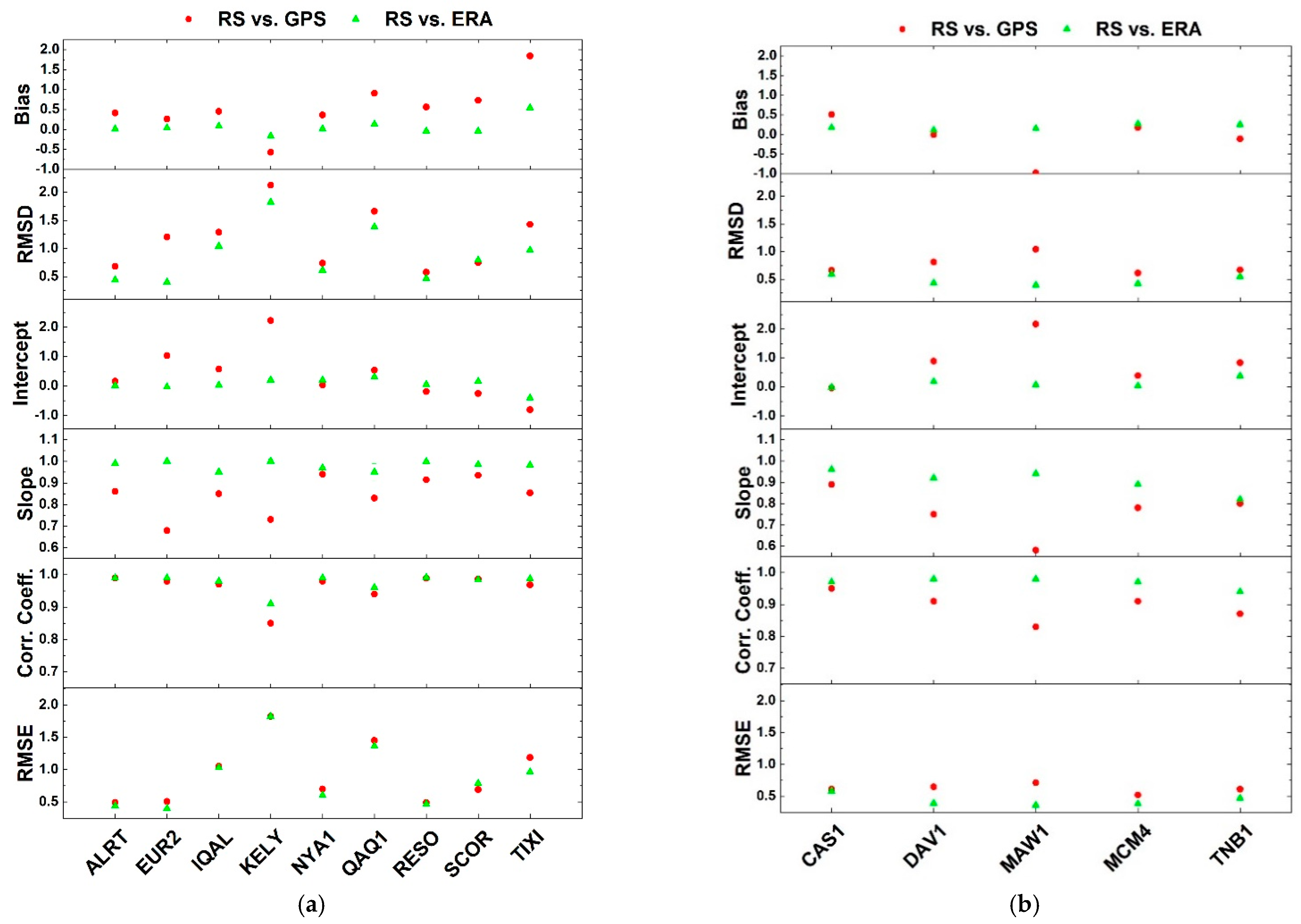
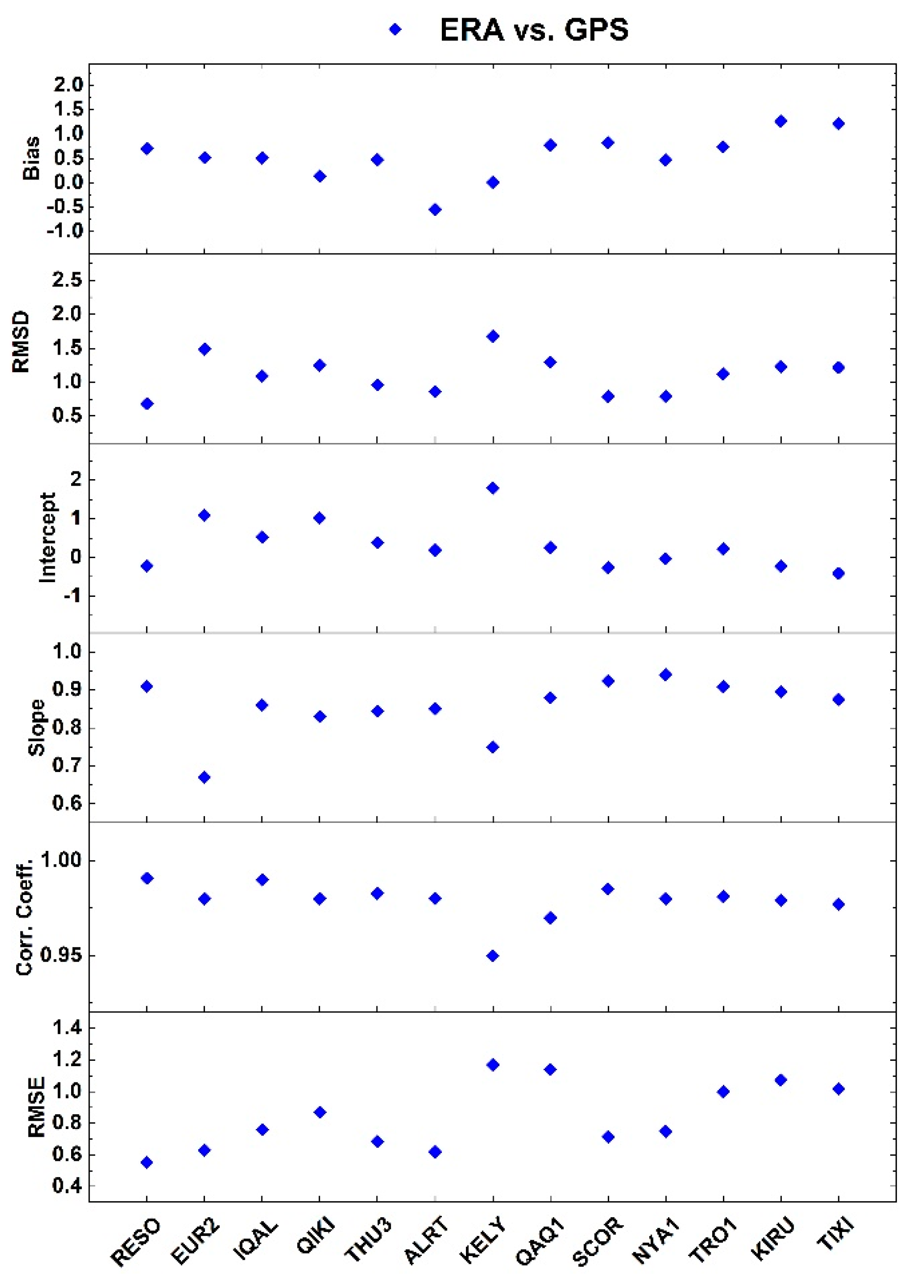
The above listed parameters estimated for the Arctic region are shown in
Figure 7a and
Table 5. As regards the bias, the RS vs. ERA comparison shows a mean value around zero, with a low negative value at KELY and a high positive value at TIXI. The greater relative bias found in TIXI can be attributed to the less effective correction procedure adopted for the corresponding radiosondes, as mentioned in
Section 2.2. The RS vs. GPS scatter plot shows positive values for the bias, except for KELY which shows a value of −0.5 mm. In both cases, the shorter time series of RS observations at KELY can affect all the results.
As regards RMSD, the values for RS vs. GPS are always higher than the RS vs. ERA values, which are on the average below 1 mm (once again, KELY is the one with the worst performance).
The intercept of the regression model indicates whether one series is drier or wetter than the other. The mean value is 0.4 mm for the GPS and ERA dataset, while it is 0.1 mm for RS vs. ERA dataset. Except for a high positive intercept value for KELY, the values are higher or lower for one dataset than the other, a symptom of uncertain behaviour.
As for the slope, the RS vs. GPS has values lower than 1 (0.8 on the average) showing bad agreement between the two series, with EUR2 and KELY the worst-performing, while the RS and ERA dataset comparison shows a very good agreement for all stations, with a mean value of 1. The better agreement between the two solutions of PW (RS and ERA) can be explained since the values from RS are assimilated in the reanalysis models, while this is not the case for the GPS ones.
The correlation coefficients are very high: 0.96 for RS vs. GPS and even more 0.98 for RS vs. ERA on the average. Moreover, in this case, KELY shows different values from those of other stations.
There are no appreciable differences for the RMSE parameter calculated for the two datasets and it is 0.9 mm on the average for both series.
The six parameters calculated for scatter plots of PW values in Antarctica are displayed in
Figure 7b and
Table 6. In this region, only 5 co-located GPS and RS stations are present, therefore the statistics are very poor. Anyway, some general comments can be made: RS vs. ERA have similar values at the different stations, while PW
GPS retrieved at MAW1 shows peculiar results. At ROTH, common data between RS and GPS are very few while none exist between RS and ERA. This evidence is probably due to the asynchronous observations between the two different techniques and, therefore, the ROTH results are not shown in the plots.
3.4. Comparison of ERA and GPS Precipitable Water at GPS Sites
All the selected GNSS stations are used in this comparison of the PW retrieval from GPS with the PW values from the ERA model (the latter is taken as the validation dataset). The scatter plots between ERA and GPS for all sites were produced, together with the graphs of the 6 parameters as defined above.
Figure 8 and
Figure 9 show the 6-parameter values for the Arctic and Antarctic stations, respectively. For the Arctic stations, the geographical criterion (stations in longitude order from Canada to Russia) was established, while for the stations in Antarctica, the orthometric height was assumed as a discriminating parameter. The stations are listed following ascending heights and 5 different zones can be emphasized: H < 500 m (from OHI2 to FTP4), 500 < H < 1 000 m (from PATN to CRDI), 1000 < H < 1500 m (from SUGG to HOWN), 1500 < H < 2000 m (from PECE to COTE) and H > 2000 m (BURI and BRIP), in order to understand whether different behaviours can be highlighted according to height.
In
Figure 8, the six parameters for the Arctic ERA vs. GPS series are displayed. As regards the bias, the comparison shows a positive mean value (0.5 mm) with a unique negative bias at ALRT. As regards RMSD, a mean value of 1.1 mm is estimated. The intercept of the regression fit shows which series appears to be drier or wetter than the other. The mean value is 0.3 mm, but except for a high positive value for KELY, the values of the other sites are fluctuating, again a symptom of uncertain behaviour. As regards the slope, ERA vs. GPS shows values lower than 1 (0.9 on the average) showing a not-optimal agreement between the two series at the different sites, with EUR2 and KELY the worst stations. The correlation coefficients are high, the mean value is 0.96, but excluding KELY, it is even higher r = 0.98. As concerns the RMSE parameter, an average value of 0.8 mm is estimated.
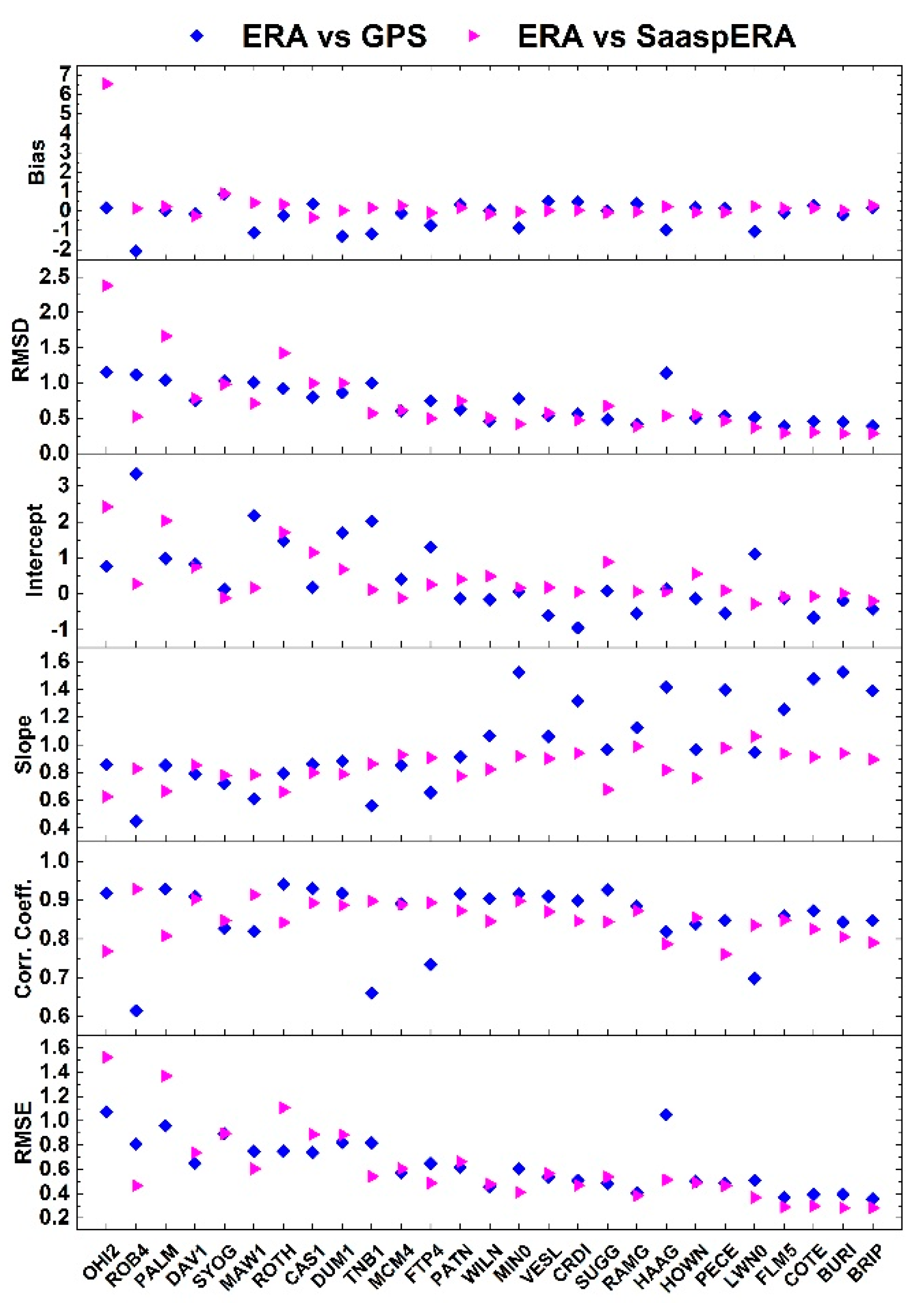
In
Figure 9, the same parameters are displayed for stations in Antarctica. A bias value of −0.2 mm is calculated, even if different values are present below and above 500 m, where it is very close to zero. The RMSD decreases with increasing height, except for HAAG. Regarding the intercept, a mean value of 0.7 mm is estimated, though above 500 m, it is close to zero. The mean of the slope has a value of 1 mm but within the single station, the slope is different if it is evaluated below or above 500 m. The Pearson’s correlation coefficients have a mean value of 0.85 as they are affected by the presence of some anomalous PW
GPS values, in particular in time series of stations ROB4, TNB1, FTP4, and LWN0. Finally, a mean value of 0.6 mm is estimated for the RMSE.
By analysing in detail the PWGPS time series, some aspects can be highlighted. Seasonal signals seem not to be present at some stations, while in some other cases, negative values of PWGPS are present. This is not physically meaningless, but it depends on how ZWD is computed, i.e., as the difference between ZTD and ZHD. A plausible explanation for negative values (case 1) could be that the a priori ZHD is not properly computed, e.g., giving higher values than the real ones. Another possible explanation (case 2) could instead be related to inappropriate ZTD estimation methods when processing GPS data.
To understand which is the most likely case, the PW was retrieved starting from the same ZTD computed during the GPS data processing, to which the ZHD value obtained using the formula proposed in Bevis et al. [
56] and Saastamoinen [
58] was subtracted:
where
ps (hPa) is the surface pressure obtained from the ERA model,
h (m) is the ellipsoidal height, and
φ (rad) the latitude of the site. The new solution is called SaaspERA. The height at which the ERA parameters were retrieved is the same as the GPS station. This analysis was performed for all selected polar stations, but the results obtained are not clear enough to give a definitive answer to the above question. In general, the new solution is worse for the Arctic stations, while in Antarctica, the results can be better or worse depending on the station. The bias is very close to zero in the scatter plot between ERA and SaaspERA, except for the station at O’Higgins (OHI2), which gets considerably worse. The mean value of RMSD is, in general, the same found for the standard solution between ERA and GPS, except for HAAG, which improves this value and some other stations that make it worse. As regards the intercept, the mean value is similar to the previous, with few stations that improve this value (ROB4, MAW1, TNB1, FTP4, LWN0) and again, some others that make it worse. The slope shows a mean value of 0.8 with less dispersion and values very close to each other among stations. The mean value of
r is similar to the standard solution, with ROB4, MAW1, TNB1, FTP4, and LWN0 that improve the
r value and some others that suffer from worse values (e.g., the stations of the Antarctic Peninsula). Finally, the RMSE value is the same as the standard solution for the majority of the stations, with few of them (ROB4, TNB1, HAAG) that show a better value and others (OHI2, PALM, ROTH) that have a worse value (see
Figure 9).
4. GPS, RS and ERA PW Time Series Analysis: Model Noise Investigations, Long Term Trend Estimation
The main purpose of this work is to provide reliable trend estimates of the PW long time series in the polar regions. To achieve this goal, time series analysis for all stations involved in this study was performed using the Hector scientific software package [
59], which allows to estimate trends from time series with temporal correlated noise. A trend analysis can be conducted by using a linear or higher degree polynomial. In addition to the possibility of identifying periodic signals, offsets, and post-seismic deformation, it handles gaps and removes outliers in the time series. Hector also estimates both the model parameters and the parameters of the chosen noise model using the Maximum Likelihood Estimation (MLE) method. If the noise model is not known a priori, as it should be, tests can be performed on the data, in order to take advantage of the best choice. The residuals were obtained by subtracting the linear trend and the seasonal signals from the time series. Furthermore, several noise-model combinations were investigated, e.g., White Noise (WN), Power Law plus White Noise (PW + WN), and autoregressive models. Among the noise combinations, the following were adopted in the daily GPS and RS time series analysis:
AR(1) = ARMA(1,0),
AR(5) = ARMA(5,0),
ARFI(1) = ARFIMA(1,0),
GGM = Generalized Gauss Markov,
PL + WN = Power Law + White Noise,
AR(1) + WN = ARMA(1,0) + White Noise.
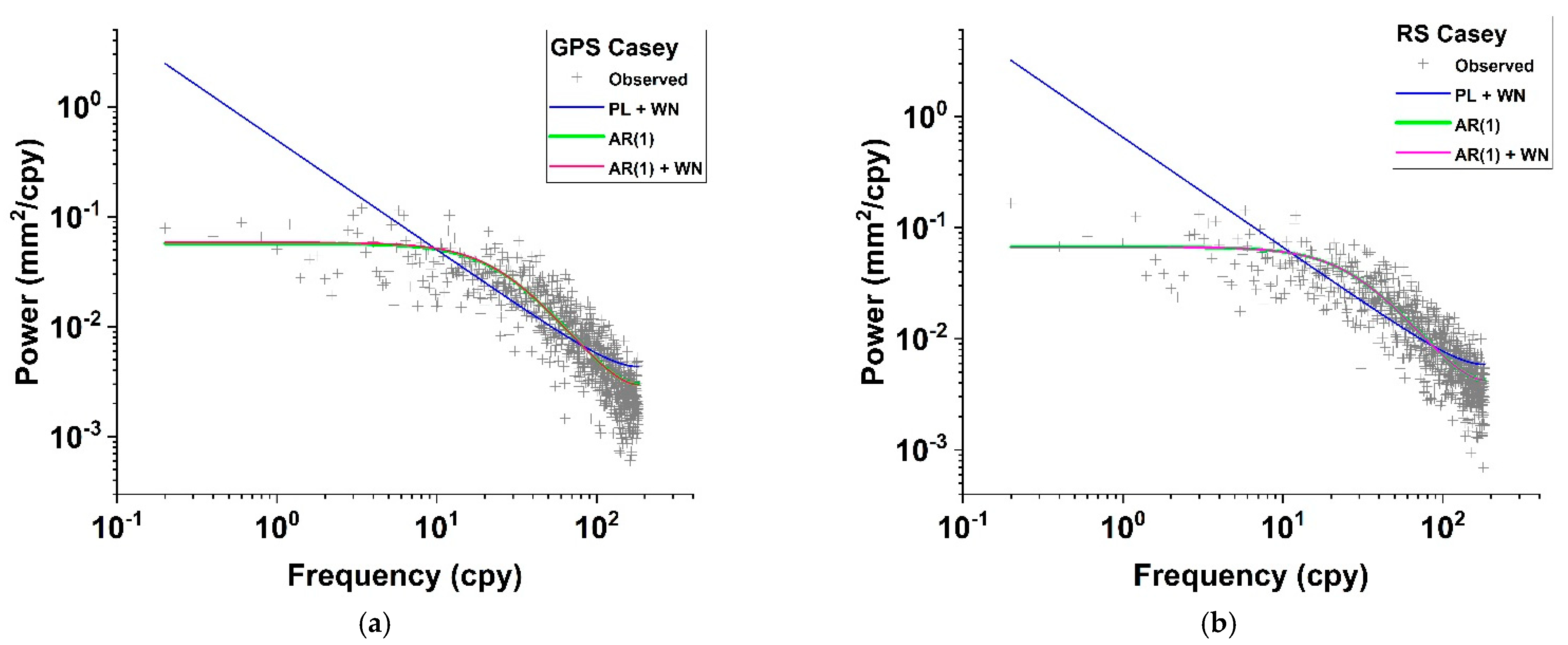
The power spectrum of the daily PW at Casey station is shown in
Figure 10a for GPS and
Figure 10b for RS. The graphs show clearly that the model PL + WN does not represent the data well, while the autoregressive models AR(1) and AR(1) + WN better fit the residuals after trend estimation; furthermore, a correct trend uncertainty is also estimated. This outcome also agrees with previous studies (e.g., [
14,
60]). The noise model AR(1) (or ARMA(1,0)) is simpler and less time consuming than others and it was adopted in this study.
The results of the Hector analysis relative to GPS, RS, and ERA daily PW time series are presented in
Table 7 and
Table 8 and
Figure 11 and
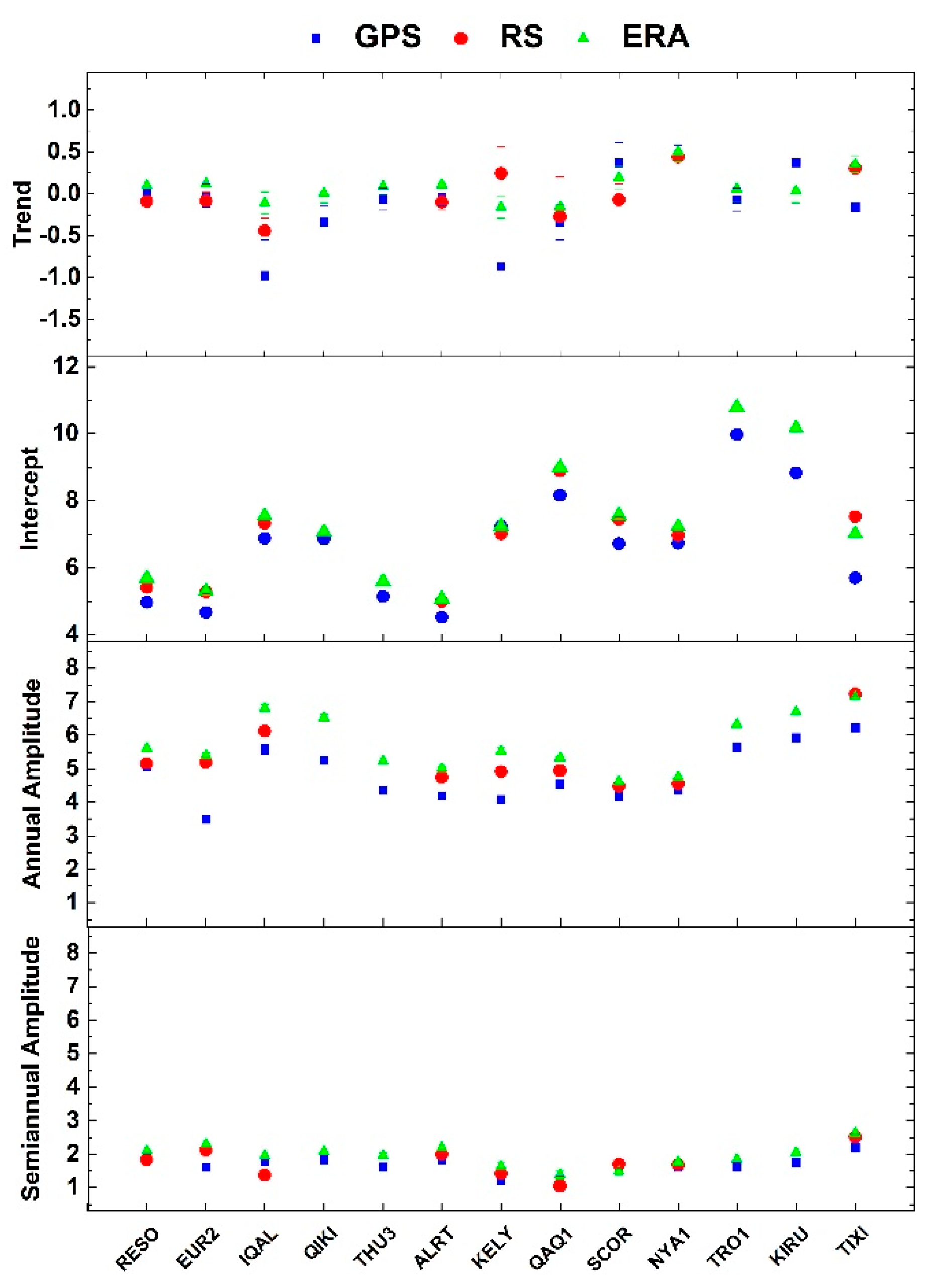
Figure 12. The parameters shown are trend (mm/decade), intercept, and amplitude of annual and semiannual signals (all in mm) with their associated errors. The intercept is equal to the estimated value in the middle of the analysed time series. Significant trends at ±1σ level according to Hector estimates are highlighted in bold in
Table 7 and
Table 8. The RS time series at Mario Zucchelli station (TNB1) is very long, but since observations are available only for summer seasons they were not deemed sufficient to provide reliable results.
In
Figure 11, trend, intercept, annual and semiannual amplitudes for PW estimates at Arctic sites are shown with reference to GPS, RS, and ERA results. The GPS trend values range from −0.98 mm/dec to 0.46 mm/dec, with a mean value of −0.10 mm/dec. RS presents a zero mean value (−0.01) mm/dec, ranging from −0.44 mm/dec to 0.44 mm/dec. Finally, ERA has an average of 0.09 mm/dec, with values from −0.16 mm/dec to 0.50 mm/dec.
There is not a clear signal of a specific technique with lower or higher values of the trend for all the stations. Looking at each site, the main discrepancies are present at KELY and IQAL, which are probably explained by the different lengths of the time series (
Table 1 and
Table 3). In any case, there is poor agreement between ERA and both GPS and RS results for either series. In some cases, GPS and RS show very similar results (ALRT, QAQ1, EUR2, RESO, NYA1). Differences are present for SCOR and TIXI, with ERA values closer to RS. If RS data are not available, no consideration can be made regarding any discrepancies between GPS and ERA data since RS has been considered the reference value in the comparison so far.
In
Table 7, the trend values are listed. Significant values (±1σ) are highlighted in bold. GPS trends are mainly negative; positive values can be found for RESO (not significant), SCOR, NYA1 and KIRU. RS shows mainly negative values, with positive trends for KELY (not significant), NYA1, and TIXI. ERA trends are more homogenous and mainly positive; the half of trends are significant and only 3 stations present negative values, 1 significant (KELY).
As for the intercept, in each station the GPS shows lower values than the other series, while the values of RS and ERA are comparable. Only for TIXI, RS presents a slightly greater value. The values range from 4.5 mm to 10.0 mm for GPS, from 5.0 mm to 8.9 mm for RS, and from 5.1 mm to 10.8 mm for ERA. Larger differences between GPS and ERA are found in KIRU, TRO1, and TIXI.
The SaaspERA solution was used to compute a new set for the above parameters at KELY station to evaluate possible improvements using this approach. However, no appreciable changes were found except for annual and semiannual amplitudes (see
Table 7).
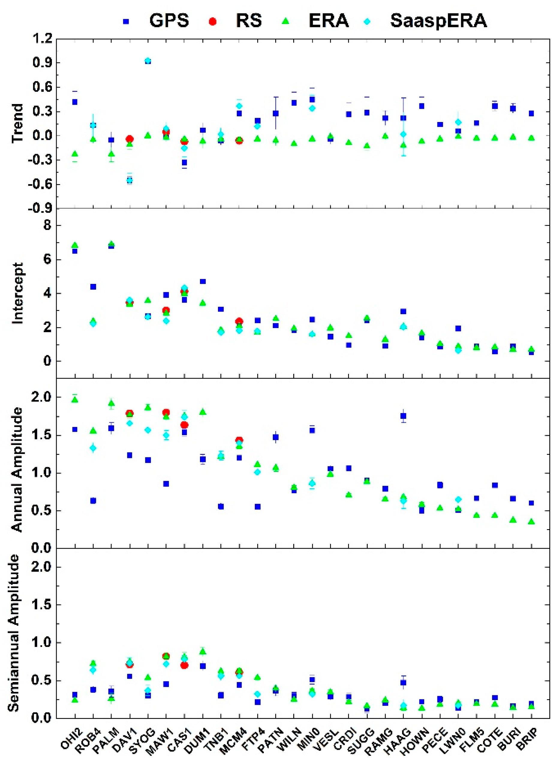
Regarding Antarctica (
Figure 12 and
Table 8), the GPS shows positive trends almost for all available stations, whereas trends of RS and ERA are negative. The mean intercept values estimated for GPS and ERA are similar, while those for RS are higher. For the latter case, it must be considered that the number of available RS stations is much lower than the GPS one. Considering only the co-located stations, trends follow the same behaviour and intercepts are very similar between the three series, while annual and semiannual values are similar for RS and ERA but lower for GPS. It should be remembered that stations with different orthometric heights show different behaviours: for H < 500 m the mean intercept is equal to 4 mm, for 500 < H < 1500 m it is 2 mm, and for H > 1500 m mean intercepts are of 1 mm or less. In the annual and semiannual amplitudes, the GPS shows values lower than those of RS and ERA. This is still true for H < 500 m, in all cases the GPS has higher values than ERA, even if the numbers involved are very small, respectively 1.7 mm and 0.6 mm.
Moreover, the SaaspERA solution was calculated for some Antarctic stations. Trends of CAS1 e HAAG definitely improve with respect to RS and ERA results, while FTP4 and MIN0 improve a little (see
Table 8 and
Figure 12). However, there is not a significant change in trend directions. As already stated, for some selected stations there is an improvement in the intercept values (ROB4, TNB1, MIN0, HAAG, LWN0, and FTP4). In addition, for the annual and semiannual amplitudes, there is a general improvement or changes not appreciable.
In any case, it can be concluded that some critical issues in the PWGPS time series are still present, in terms of hourly PWGPS negative estimated values, which, in some cases, are not solved with the SaaspERA solution. This means that our data analysis fails for the inner areas of Antarctica and further investigations will be needed to better clarify this argument. However, in terms of trend estimation, the GPS solutions are validated for providing valuable results.
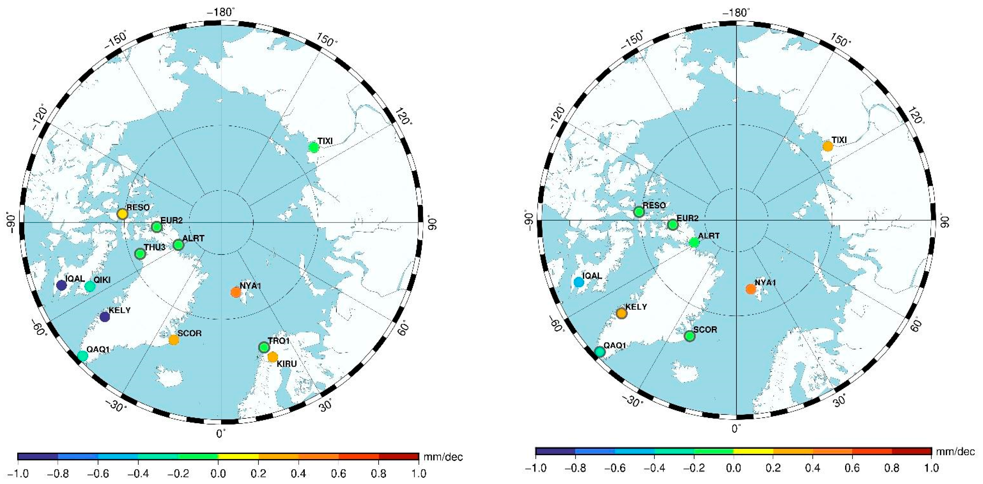
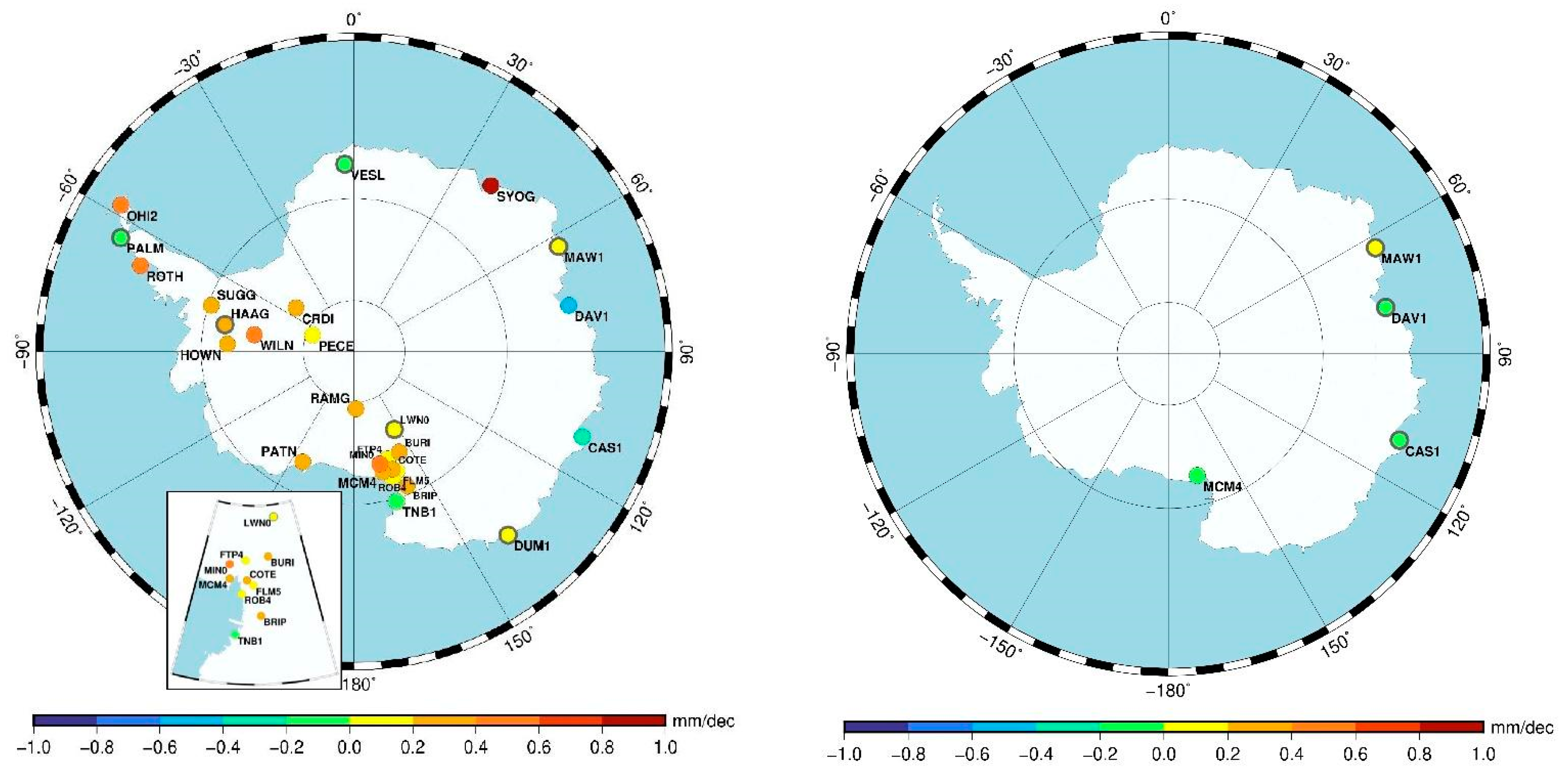
PW trends estimated at GPS and RS stations from PW time series are shown in
Figure 13, superimposed to Arctic and Antarctic geographical areas.
Negative PW
GPS trends dominate in the Arctic with the strongest PW
GPS decrease at IQAL and KELY (−1.0 mm/dec and −0.9 mm/dec, respectively). Positive PW
GPS trends can be noted at NYAL, KIRU, and SCOR (~0.4 mm/dec) sites placed in the Atlantic Ocean zone. The sites located at higher latitudes show no significant values (at 1σ level). A similar distribution of the PW
RS trends in the Arctic can be seen in the upper right panel of
Figure 13. The distribution of PW
GPS and PW
RS trends in the Arctic shows that the stations in the sector between Greenland and North America are predominantly characterized by negative trends, while those in the Atlantic Ocean region show predominantly a positive trend. These findings are consistent with the results obtained by Tomasi et al. [
29], who analysed the PW extracted from RS data collected for 14 Arctic sites, including some of the stations used in the present study. Similarly, a long-term decrease in PW was found at Greenland and North American sites and a long-term increase at stations from the Atlantic Ocean to the coasts of Central Siberia.
The positive trend of PW in the Atlantic sector was also reported by many authors (Rinke et al. [
30] and references therein) and believed to be responsible for the increase in air and sea surface temperature (SST), advection of humidity, and reduction in the extent of sea ice. It should be also pointed out that the warm waters of the tropics, which are carried north across the Atlantic Ocean by the Gulf Stream, contribute to maintain relatively high temperatures in the waters of the Norwegian and Barents seas [
61]. Carvalho and Wang [
62] studied the SST variability in the Arctic Ocean during the 1982–2018 period and found positive SST trends between 0.2 °C/dec and 0.8 °C/dec in the coastal zones of the Norwegian, Barents, and Kara seas, while the trend on the Canadian coasts and around Greenland was mostly close to zero. While the Arctic Ocean and surrounding seas significantly affect the environment in the North Pole area, the distribution of the PW trend in the Arctic obtained in this study could be associated with the SST trends reported by Carvalho and Wang [
62].
Cox et al. [
63] concluded that the humidity trends play an important role in the radiative budget of the Arctic surface and, especially, they can influence the clouds’ radiative effect. Hence, knowledge about these trends improves our understanding of climate change, which implies the importance of humidity monitoring over large Arctic areas.
The lower row of
Figure 13 indicates that the stations in the West Antarctic sector show a predominantly positive PW
GPS trend (from 0.1 mm/dec to 0.7 mm/dec), while the sites on the coastal zone of the East Antarctic exhibit a few significant PW
GPS (from −0.1 mm/dec to −0.4 mm/dec) and predominantly no significant PW
RS trends. Some researchers [
11,
64] reported positive near-surface temperature trends in the West Antarctic and trends with a doubtful significance on the coasts of the East Antarctic. Since the increase in temperature near the surface usually leads to an increase in humidity and therefore in PW, as assumed for the Arctic, the results given in the lower row of
Figure 13 can be considered consistent with the findings presented in the above research studies.
Other authors reported global or regional PW trends (e.g., [
17]). For the only six common sites, our results are different from those of Parracho et al. [
17], in some cases the trends are even opposite for both GPS and ERA. This may be due to the different observation periods and/or for different sampling (hourly compared to monthly solutions).
5. Conclusions
This work is focused on the evaluation of PW in the polar regions and on the estimation of its trend through the analysis of long time series from different sources. Particular attention was paid to Antarctica, where data are scarce and generally difficult to collect. The observations acquired at the permanent Antarctic GNSS stations, which are maintained by various institutions and included in the international and regional networks (IGS, POLENET and VLNDEF), were analysed.
A global network of more than 200 stations, some with 20-year GPS records, was analysed to ensure the maximum accuracy of the time series by adopting a homogeneous, coherent, and up-to-date processing strategy. To this aim, the Bernese GNSS software was used together with models and a priori information capable of providing the Zenith Wet Delay (ZWD), even where local surface meteorological data were not available.
Among them, 40 geodetic GNSS stations were selected to retrieve hourly precipitable water (PW) values. Some of these stations are co-located with Radio Sounding (RS) stations, where Vaisala sensors are used to collect atmosphere pressure, temperature, and relative humidity. The meteorological parameters, appropriately corrected for the main lags, instrumental errors, and the various dry biases, were used to obtain homogenous long time series of PWRS. As an additional tool for validation and comparison of the results, the global atmospheric reanalysis ERA-Interim was also used for all the selected GPS stations. A small dry bias of RS vs. GPS values was found in the Arctic, while no clear behaviour is present in Antarctica. Since various correction procedures were applied to the RS data, they could be considered a standard to some extent. Nevertheless, the discrepancy between PWRS and PWGPS should be carefully examined to better understand the sources of error in both approaches, once more data and co-located stations are analysed, especially in Antarctica.
The PWGPS and PWRS seasonal variations are consistent, as also confirmed by scatter plots and related correlation coefficients, and show values, on average, of 0.96 for RS vs. GPS and 0.98 for RS vs. ERA in the Arctic and 0.89 for RS vs. GPS and 0.97 for RS vs. ERA in Antarctica.
Once validated, long-term trends for both Arctic and Antarctic regions were estimated using the scientific software package Hector, which allows the estimation of trends from time series with temporal correlated noise. We applied a function to estimate the linear trend plus the annual/semiannual signals, and autoregressive noise model AR(1) which best fits the residuals of all investigated PW time series. The choice of the most suitable noise model was also fundamental in determining the residuals of the time series, once the trend and seasonal signals were subtracted.
Both PWGPS and PWRS trends in the Arctic show that the stations in the sector between Greenland and North America are predominantly characterized by negative trends (from −1.0 to −0.3 mm/dec), while those located in regions bordering the Atlantic Ocean show predominantly a positive trend (~0.4 mm/dec). Regarding Antarctica, the stations in the West Antarctic sector show a predominantly positive PWGPS trend (from 0.1 mm/dec to 0.7 mm/dec), while the sites on the coastal zone of the East Antarctic exhibit only few significant PWGPS trends (from −0.1 mm/dec to −0.5 mm/dec), and predominantly no significant PWRS trends.
The values of PW trends estimated in polar regions are extremely small and longer time series would be needed to provide more reliable values. We are planning to reprocess the GPS data as soon as the ITRF2020 is available along with the relevant IGS products. Meanwhile, an increase in the number of GNSS stations with a longer observation time interval is expected. This will allow us to obtain more reliable results and extend the number of long-term trends suitable for climate-related studies.


 ,
, 


