Abstract
Snow preserves fresh water and impacts regional climate and the environment. Enabled by modern satellite Earth observations, fast and accurate automated snow mapping is now possible. In this study, we developed the Automated Snow Mapper Powered by Machine Learning (AutoSMILE), which is the first machine learning-based open-source system for snow mapping. It is built in a Python environment based on object-based analysis. AutoSMILE was first applied in a mountainous area of 1002 km2 in Bome County, eastern Tibetan Plateau. A multispectral image from Sentinel-2B, a digital elevation model, and machine learning algorithms such as random forest and convolutional neural network, were utilized. Taking only 5% of the study area as the training zone, AutoSMILE yielded an extraordinarily satisfactory result over the rest of the study area: the producer’s accuracy, user’s accuracy, intersection over union and overall accuracy reached 99.42%, 98.78%, 98.21% and 98.76%, respectively, at object level, corresponding to 98.84%, 98.35%, 97.23% and 98.07%, respectively, at pixel level. The model trained in Bome County was subsequently used to map snow at the Qimantag Mountain region in the northern Tibetan Plateau, and a high overall accuracy of 97.22% was achieved. AutoSMILE outperformed threshold-based methods at both sites and exhibited superior performance especially in handling complex land covers. The outstanding performance and robustness of AutoSMILE in the case studies suggest that AutoSMILE is a fast and reliable tool for large-scale high-accuracy snow mapping and monitoring.
1. Introduction
Snow is one of the most common land covers [1]. As a major source of Earth surface fresh water, snow melts into water and runs to rivers and lakes, consequently impacting drinking water supply, regional ecosystem [2], agriculture [3], and the climate at large. Therefore, fast and accurate mapping of snow cover is essential for monitoring natural resources, regional climate change and environment evolution [4]. Owing to the fast growth of Earth observation (EO) data, frequent monitoring of large-scale snow covers becomes possible.
Visual interpretation features high accuracy but requires a tremendous amount of time and effort, especially when dealing with large areas [5]. Apart from visual interpretation, many existing studies apply rule-based methods for fast extraction of snow areas [6,7,8,9]. The National Aeronautics and Space Administration (NASA) uses multiple thresholds for different bands and the normalized difference snow index (NDSI) to produce the fifth collection of Moderate Resolution Imaging Spectroradiometer (MODIS) snow products [10], with the highest resolution of 500 m. Gascoin et al. launched the Theia snow collection to provide high-resolution (20/30 m) snow products for the mountain regions in western Europe (e.g., Alps, Pyrenees) and the High Atlas in Morocco using multiple thresholds on DEM and indices calculated from Sentinel-2 and Landsat-8 images [9]. Although rule-based methods exhibit good capabilities in mapping snow of some regions [11], the best thresholds or configurations vary significantly with space and time [7], and a set of universally applicable snow mapping parameters can hardly be defined.
Unlike the threshold methods at pixel level, object-based methods analyze the land cover through objects, which are essentially groups of pixels segmented by algorithms. Object-based methods have been proven effective in many land cover classification studies [12,13], and perform even better than pixel-based methods [14,15]. For instance, Rastner et al. [15] found that an object-based analysis has overall a ~3% higher quality than a pixel-based analysis when conducting glacier mapping. However, very limited attempts have been made in advancing object-based snow mapping [16]. Wang et al. [16] conducted snow mapping using both pixel- and object-based information. Also, commercial software like eCognition is heavily relied upon in object-based studies [12,13,16].
Machine learning (ML) has been proven to be a powerful tool in many recent Earth science applications [17,18,19,20]. Accordingly, researchers started to develop ML-based methods for snow mapping [21,22,23,24,25,26]. Liu et al. [22] compares three machine learning algorithms in improving the accuracy of the MODIS daily fractional snow cover in the Tibetan Plateau. Liu et al. [26] used a principal component analysis–support vector machine (PCA–SVM) method to estimate snow cover from the MODIS and Sentinel-1 SAR data. Cannistra et al. [25] used convolution neural network (CNN) to map high-resolution snow covered areas using the PlanetScope optical satellite image dataset. These studies, however, barely explored the use of machine learning in object-based snow mapping. Therefore, three crucial challenges remain unaddressed: (a) object-based snow mapping using machine learning has not been attempted; (b) open-source solutions for object-based automated snow mapping need to be developed; and (c) the benefits of using auxiliary data in snow mapping are yet to be confirmed.
Accordingly, the main objectives of this study are to develop a Python-based open-source automated snow mapper for fast and accurate snow mapping using EO products, as well as to investigate ML-based solutions for object-based snow mapping with auxiliary data. The key novelty and contribution of this study lie in the fact that it is the first work that combines machine learning with object-based analysis in snow mapping. Equally important, it presents the first machine learning based open-source system for large-scale automated snow mapping.
2. Materials and Methods
2.1. Study Area
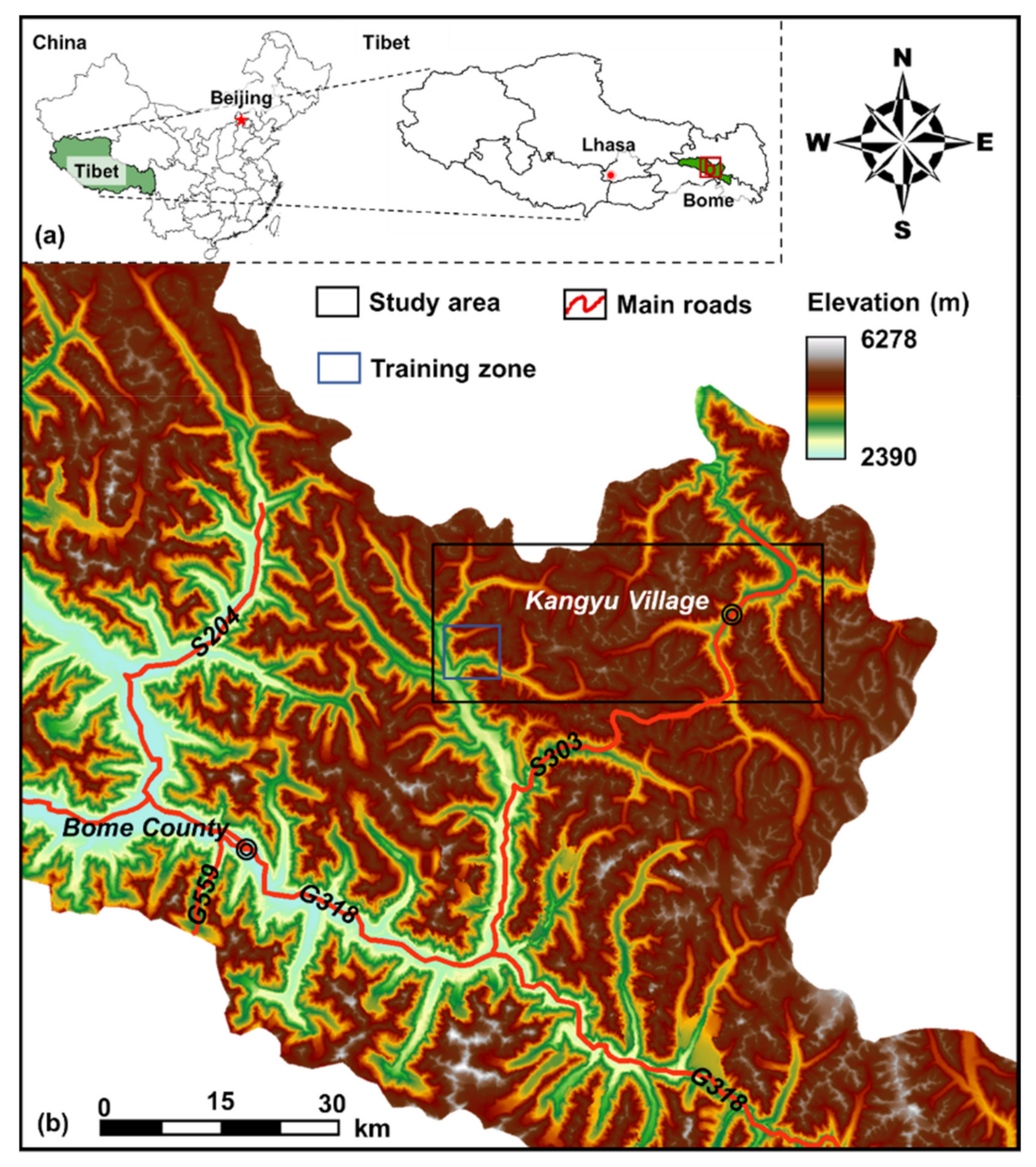
The study area is located at the northeast of Bome County, Tibet, China (Figure 1), covering a total area of 1002 km2. With a high average altitude of 4720 m, the study area is partially covered by perennial snow. The maximum elevation difference within the study area reaches 2228 m, indicating a typical alpine-gorge landform of the Sichuan-Tibet region. According to the weather records of China Meteorological Administration (CMA) from 1981 to 2010, the annual average temperate of Bome is 9 ℃, with a lowest monthly average of 0.7 ℃ in January and a highest average of 16.9 ℃ in August. The winter of Bome is long (October to March) while summer is usually absent. Bome has a humid monsoon climate with annual relative humidity of 71.2% and annual rainfall of 890.9 mm. Several key infrastructural projects are located in the study area, such as the Sichuan–Tibet railway and Provincial Road S303.
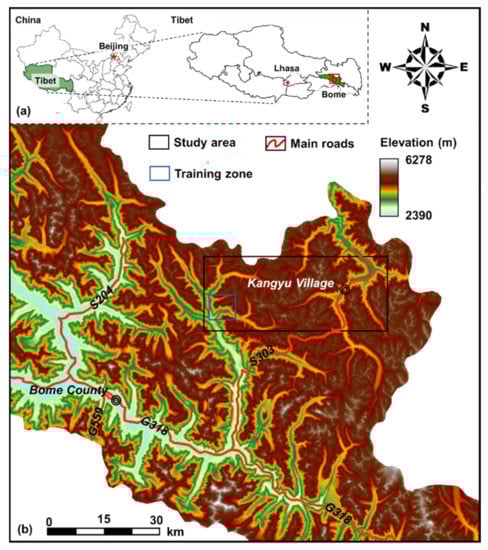
Figure 1.
Locations of (a) Bome County and (b) the study area on a digital elevation map. (Source of the digital elevation model: National Aeronautics and Space Administration Shuttle Radar Topography Mission Global 1 arc second product).
2.2. Data
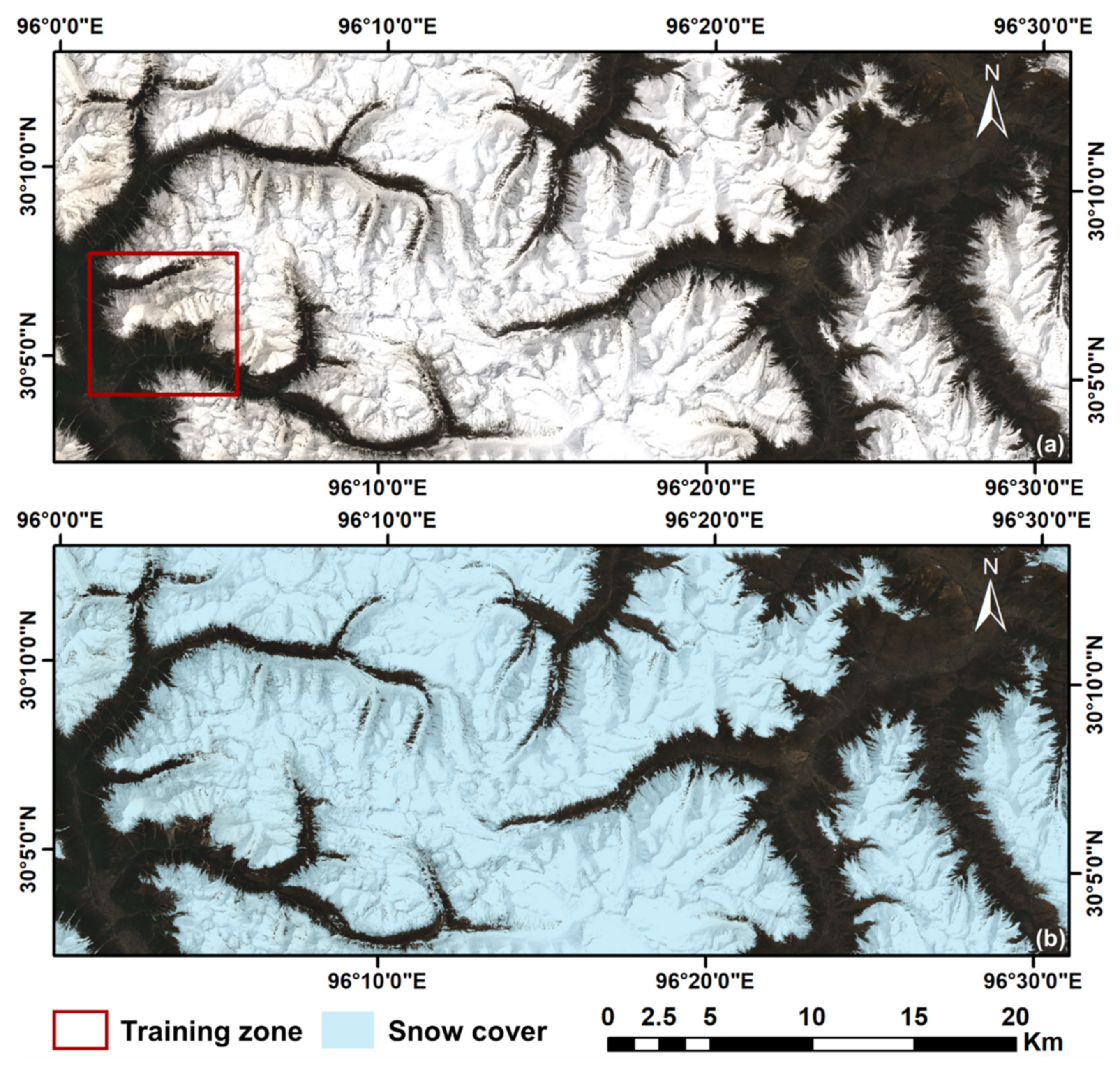
A multi-spectral Level-1C product of Sentinel-2B, which was captured on 30 April 2021, was acquired and used in this study for snow mapping (Figure 2a). The Sen2Cor processor developed by the European Space Agency (ESA) was first used to generate the Level-2A product by performing atmospheric corrections on the original product. A multi-spectral product of Sentinel-2B has thirteen bands: four bands with 10 m spatial resolution (Blue, Green, Red and Near Infra-Red bands), six with 20 m spatial resolution (Red Edge 1, Red Edge 2, Red Edge 3, Narrow Near Infra-Red, Short Wave Infrared 1 and Short Wave Infrared 2 bands) and another three with 60 m spatial resolution (Coastal Aerosol, Water Vapor and Cirrus bands). In order to have a uniform spatial resolution for feature extraction, Sen2Res, a processor recommended by the ESA, is used to enhance the spatial resolution of low-resolution bands to 10 m. Sen2Res uses a super-resolution method proposed by Brodu [27], which utilizes shared information between bands and band-specific information, to produce super resolution products. After resolution enhancement, the spatial resolutions of all bands increase to 10 m except Coastal Aerosol, Water Vapor and Cirrus bands. The three bands are not used in this study due to their insufficient original resolution (60 m) and intended purposes (the Coastal Aerosol band for aerosol retrieval, the Water Vapor band for water vapor correction and the Cirrus band for cirrus detection). Detailed band statistics and information of the 13 bands within the study area are summarized in Table 1. In the case of cloud presence, the cloud mask which comes with each Sentinel-2 product can be used to remove cloud areas.

Figure 2.
(a) True-color red, green and blue (RGB) image of the study area in Bome County and the location of training zone and (b) pixel-level snow cover of the study area based on visual interpretation.

Table 1.
Band information and statistics of the multispectral image of the study area in Bome County.
Based on the true color image shown in Figure 2a, which is composed of red, green and blue channels, a pixel-level snow cover inside the study area was manually interpreted and presented in Figure 2b. A small part of the study area is chosen as the training zone (red box in Figure 2a) and the rest of the area is used for model testing. With the intention of developing a universally applicable tool which can be trained with limited data but predict accurately for a large area, the training zone is purposely set to only occupy approximately 5% (50.4 km2) of the entire study area (1002 km2).
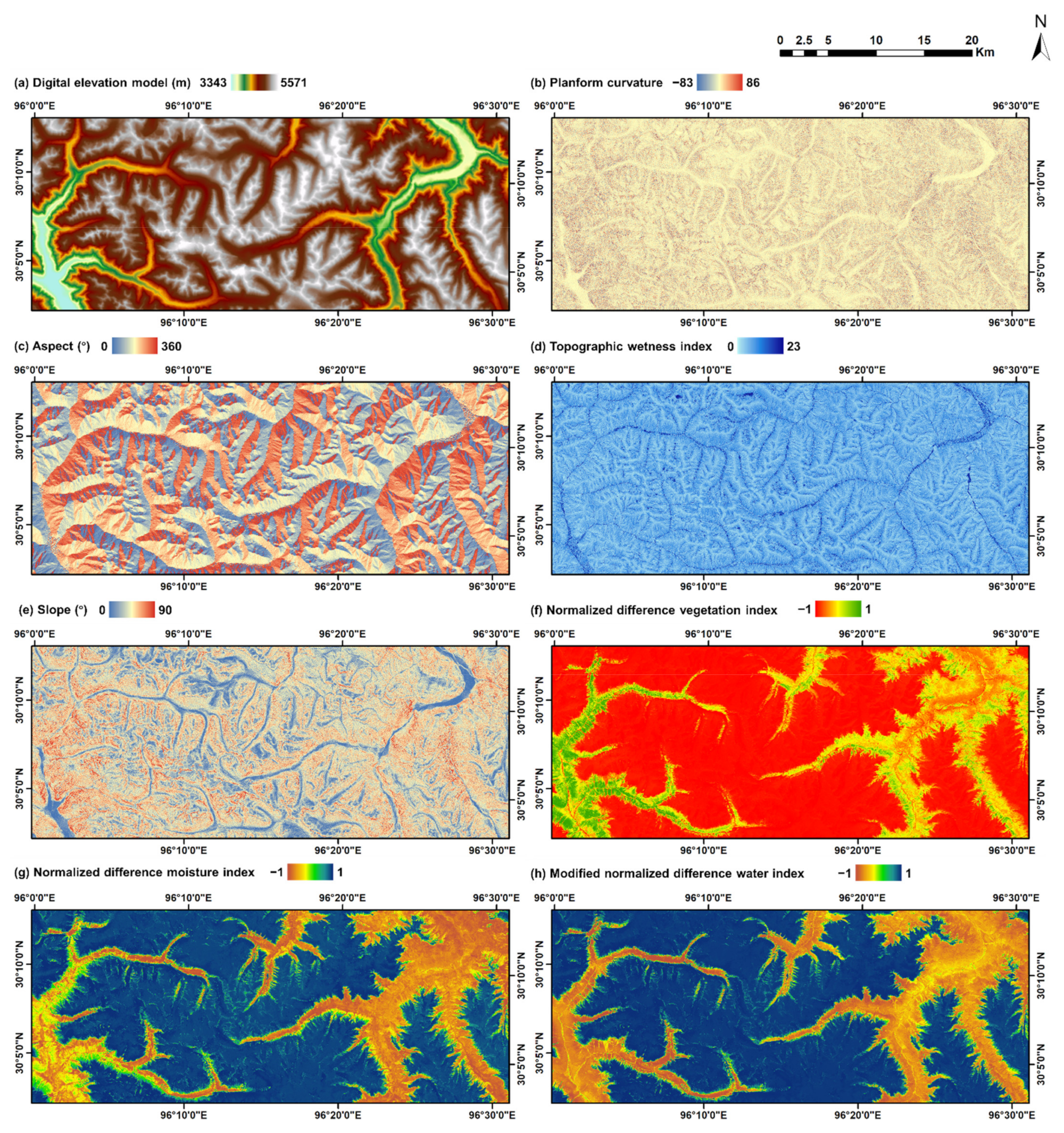
Other than the multi-spectral data, we also examined the contribution of auxiliary data in snow mapping. Thus, two kinds of auxiliary data are collected in this study and shown in Figure 3; namely, a digital elevation model (DEM) and its derivatives, and spectral band-derived data. The DEM data of 12.5 m resolution of the study area is collected from the Radiometric Terrain Correction (RTC) product created by the Alaska Satellite Facility (ASF), which originated from the NASA Shuttle Radar Topography Mission (SRTM) Global 1 arc second product. It is then resampled to 10 m using the nearest neighbor method (Figure 3a). Four widely used derivatives are then produced to describe the topographic characteristics of the study area; namely, planform curvature (Figure 3b), aspect (Figure 3c), topographic wetness index (TWI, Figure 3d) [28] and slope (Figure 3e). The normalized difference vegetation index (NDVI, Figure 3f), normalized difference moisture index (NDMI, Figure 3g) [29] and the modified normalized difference water index (MNDWI, Figure 3h) [30] are chosen as the band-derived indices to provide additional information about the land cover. The three indices are given by:
where NDVI is a common indicator of surface plant health; NDMI is sensitive to moisture levels in vegetation; and MNDWI, also known as the normalized difference snow index (NDSI), is generally used to enhance the open water features or identify snow cover.
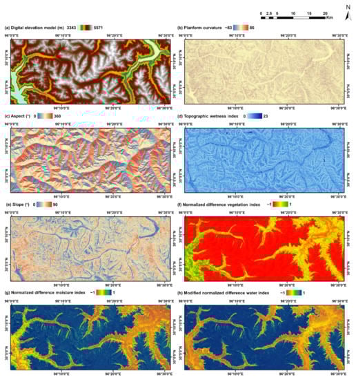
Figure 3.
Data layers of the study area: (a) digital elevation model; (b) planform curvature; (c) aspect; (d) topographic wetness index; (e) slope; (f) normalized difference vegetation index (NDVI); (g) normalized difference moisture index (NDMI) and (h) modified normalized difference water index (MNDWI). (The digital elevation model is acquired from the Alaska Satellite Facility Distributed Active Archive Center and originated from the National Aeronautics and Space Administration Shuttle Radar Topography Mission Global 1 arc second product. The Sentinel-2B multi-spectral image, which is used to produce the NDVI, NDMI and MNDWI layers, is acquired from the Copernicus Open Access Hub of the European Space Agency).
2.3. AutoSMILE: Automated Snow Mapper Powered by Machine Learning
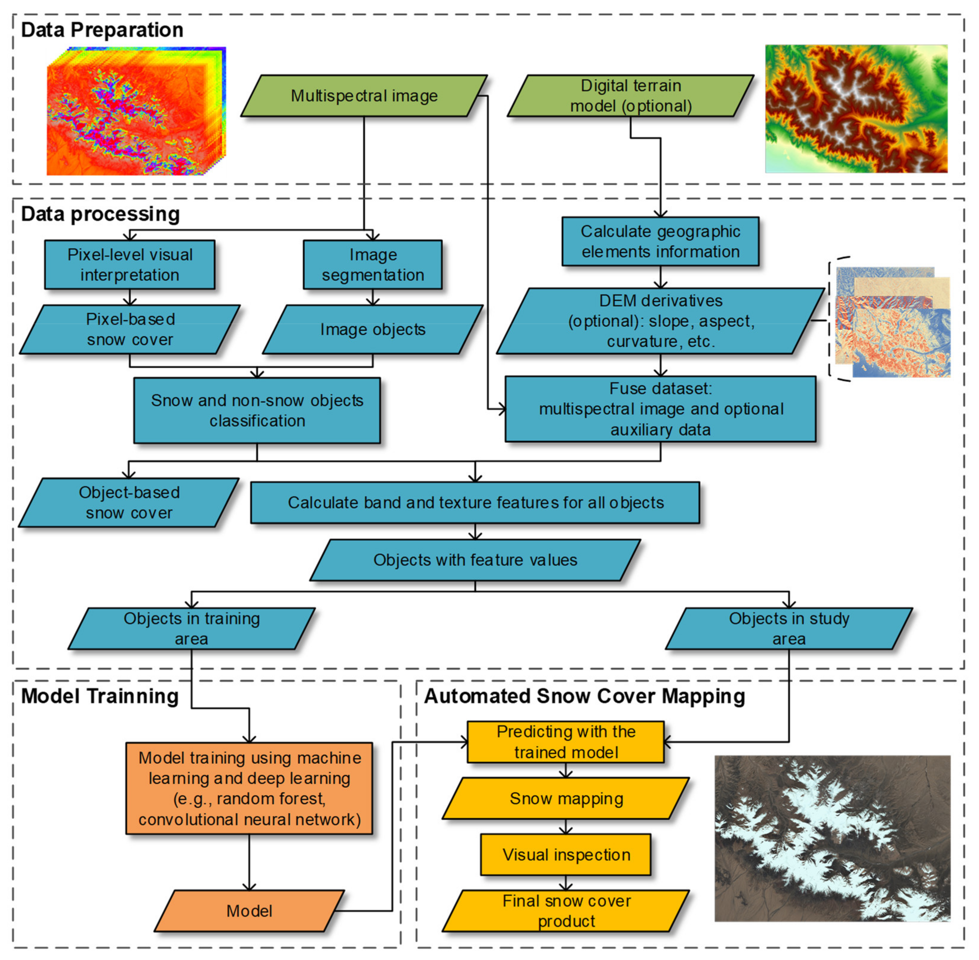
In this study, we developed the system AutoSMILE (Automated Snow Mapper Powered by Machine Learning) with open-source packages in the Python 3.8 environment, to automate the process of snow mapping. As shown in Figure 4, AutoSMILE consists of three main modules; namely, a data processing module that includes image segmentation and feature extraction, a model training module that applies machine learning and deep learning and a snow mapping module that conducts snow mapping with trained models and visual inspection. Technical details of these modules will be introduced in the following sections.
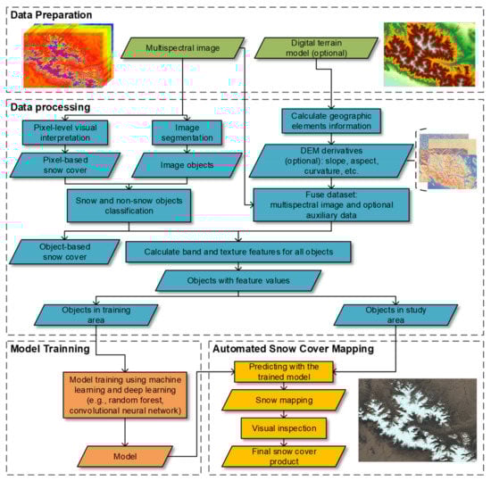
Figure 4.
Framework of AutoSMILE (automated Snow Mapper Powered by Machine Learning).
2.3.1. Image Segmentation
Image segmentation is the first step after data preparation. In AutoSMILE, the quickshift mode-seeking algorithm proposed by Vedaldi and Soatto [31] is employed, which is available in the scikit-image package (https://scikit-image.org/, accessed on 30 September 2021). Given a set of data points, the goal of a mode-seeking algorithms is to locate the maxima (i.e., modes) of the density function estimated from the set of data. Quickshift, which computes a hierarchical segmentation on multiple scales concurrently, is essentially a modified version of traditional mean-shift algorithm. Given N data points x1, …, xN, quickshift starts by computing the Parzen density estimate P(x):
where k(x) is a kernel function, which is often in the form of a Gaussian window. D(xi, xj) is the distance function between xi and xj. Then, quickshift moves each point xi to the nearest neighbor for which there is an increment of density P(x) and subsequently connects all the points to a single hierarchical tree. By breaking the branches of the tree that are longer than a certain threshold, modes can be recovered and used for image segmentation.
In the quickshift function of scikit-image, two key parameters, which control the segmentation process, can be identified; namely, the kernel size (KZ) and maximum distance (MD). KZ controls the width of Gaussian kernels used in local density approximation and MD is the threshold that decides the level in the hierarchical segmentation. The impact of different values of KZ and MD on AutoSMILE’s performance is also investigated and discussed in Section 3.1. Other parameters in this function (e.g., ratio and sigma) remain at their default values. The image segmentation is conducted on the true-color image of the study area (Figure 2a). After the quickshift segmentation, similar pixels share the same mode, gather together and form objects. Note that an object is inherently a group of similar pixels.
2.3.2. Object Labelling and Feature Extraction
The label of each object is assigned based on the manually interpreted pixel-level snow cover (Figure 2b). First, the label of each pixel is determined by whether its location falls in the snow area. Then, a simple strategy is applied in AutoSMILE: objects with more than 50% of snow member pixels are assigned with snow object labels; otherwise, non-snow labels are given. Note that it is inevitable some objects contain both snow and non-snow pixels. Thus, the snow covers mapped by snow objects and snow pixels, so called object-based and pixel-based snow covers, will be slightly different and the difference is defined as the segmentation loss. Assume that an image has W × L pixels. After certain segmentation, M objects are created. Each object i has ni member pixels and the fraction of snow member pixels is Pi. Then the segmentation loss of the object-based snow cover can be defined as:
As the data layers are already prepared at a uniform resolution (10 m in this study), the values of member pixels of a certain object can be easily extracted from different data layers to calculate object features. To fully characterize objects, AutoSMILE creates both high-level band and texture features for each object. The band features, which are calculated band-wise, include the minimum, maximum, mean, variance, skewness and kurtosis of the member pixels’ values of an object. Regarding the texture features, AutoSMILE uses the Haralick method [32] to calculate the grey-level co-occurrence matrix (GLCM) of an object. Based on the GLCM, four-directional (i.e., 0°, 45°, 90° and 135°) contrast, dissimilarity, homogeneity, angular second moment (ASM) and correlation are calculated using the scikit-image package. In this study, texture features are calculated based on red, green and blue bands. Thus, each object will obtain six band features from each layer and 20 more texture features (five features in each direction) if the red, green or blue band is encountered.
2.3.3. Machine Learning and Deep Learning
Under the proposed framework of AutoSMILE, the snow mapping problem is treated as a binary classification task and no particular machine learning or deep learning algorithm is required. In this study, we select one popular machine learning algorithm (i.e., random forest, RF) and one well-known deep learning algorithm (i.e., convolutional neural network, CNN) due to their outstanding performance and robustness in various applications [33,34].
RF, as an ensemble algorithm, is developed on the basis of decision trees and bagging [35]. In classification tasks, the output of RF is the class voted by the majority of the trees. The major improvement of RF is that it decorrelates the trees in it by only selecting a random subset of the features at each candidate split when constructing each decision tree. A typical practice is to randomly choose (rounded down) features at each split for a classification task with p features.
CNN is a popular deep learning algorithm in computer vision [36]. It is good at feature extraction and usually consists of four types of layers: convolutional layers that use a set of convolutional filters to activate certain features from the input; activation layers like the rectified linear unit (ReLU) to accelerate the training process; pooling layers which simplify the output by non-linear downsampling and other basic layers such as the fully connected layers and flatten layers. In this study, the input is taken as a ‘long’ picture with unit width to apply CNN for feature learning and snow mapping.
2.3.4. Performance Evaluation and Post-Processing
Trained machine learning models are then used for mapping snow for the entire study area. Four popular machine learning performance indices in remote sensing are selected to evaluate the performance of trained models; namely, producer’s accuracy (PA), user’s accuracy (UA), intersection over union (IoU) and overall accuracy (OA). Definitions of the four indices are given as follows:
where TP (true positive) and FP (false positive) are the numbers of correct and incorrect positive/snow predictions. Similarly, TN (true negative) and FN (false negative) stand for the numbers of correct and incorrect negative/non-snow predictions, respectively. PA, also known as recall, is the percentage of TP predictions among all positive samples. UA quantifies the fraction of TP predictions among all samples predicted to be positive, which is also known as precision. IoU measures the ratio of the intersection between ground truth snow area and predicted snow area over their union. Due to the presence of two sets of ground truths: object- and pixel-based snow covers, the snow cover mapped by the trained ML model is compared with the two snow covers. The object- and pixel-based performance indices are then calculated, which reflect the model performance at different levels.
The final step of AutoSMILE is visual inspection to ensure the snow mapping is satisfactory and to make necessary corrections before exporting the final snow cover product.
3. Results
3.1. Snow Mapping Results from Different Segmentations
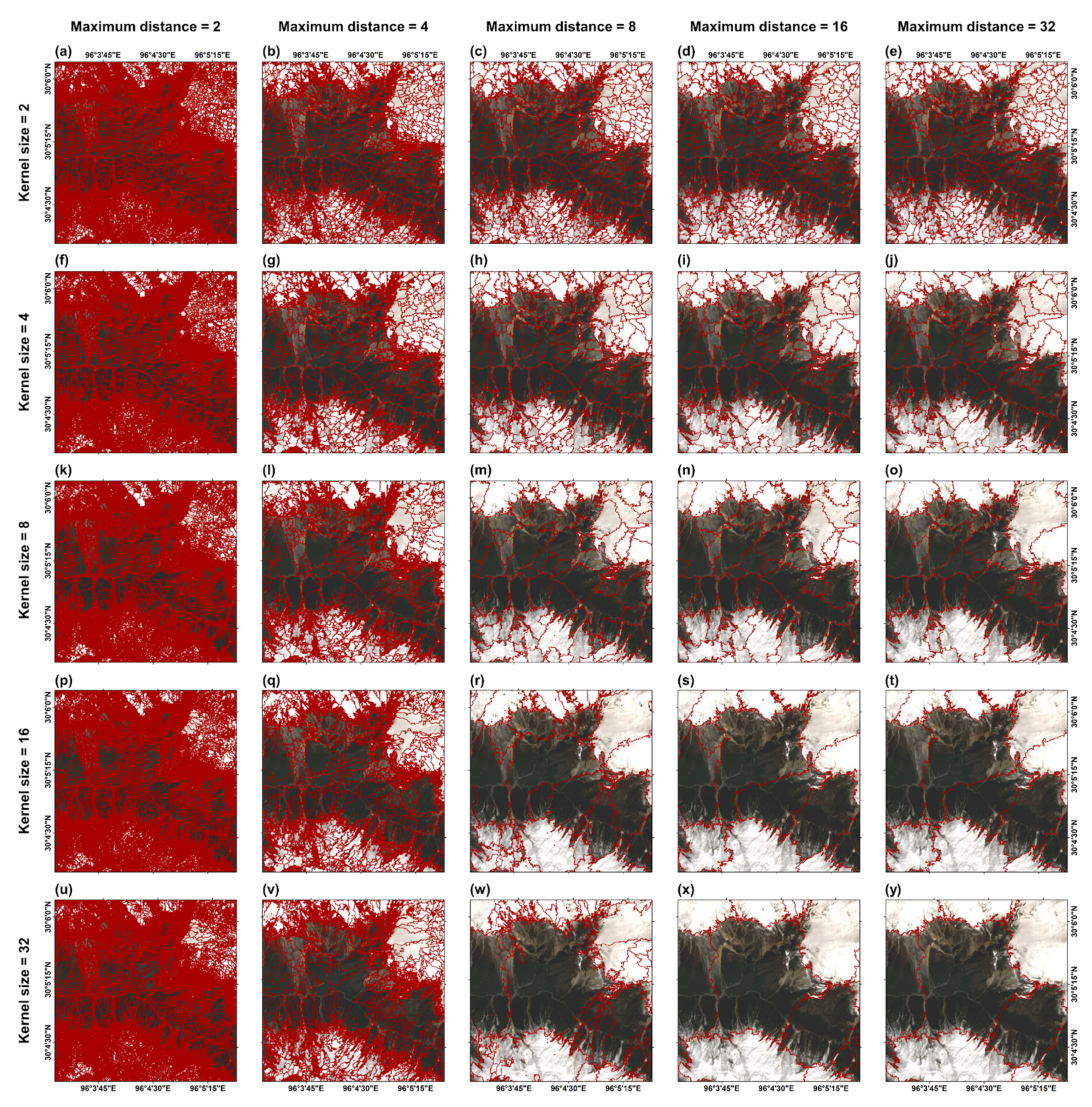
To investigate the influence of segmentation parameters on AutoSMILE’s performance, different combinations of KZ and MD are tested. Table 2 summarizes the numbers of objects given by different combinations. It can be found that a low MD will lead to a large number of objects and that the object number drops rapidly with an increase in MD. For example, when MD increases from 2 to 8, the maximum decrease of the object number reaches 99.5%. In contrast, KZ has a much less effect on the object number. In most cases, a higher KZ tends to have fewer objects. Figure 5 compares different segmentations that are mapped in a subarea of the training zone. The boundaries of objects produced with a higher MD overlap those of the objects produced with a lower MD. This is because MD controls the segmentation hierarchical level: objects segmented with higher MDs are inherently produced by merging objects segmented with lower MDs. In the cases of MD = 2 and 4, excessive oversegmentation can be observed as a large number of unnecessary small objects are created inside the same land cover. In view of computational efficiency, when the object number exceeds 100,000, AutoSMILE will slow down as object feature computation will require more resources. Thus, according to Table 2, quickshift with too small MDs (<8) is usually not recommended in AutoSMILE. When increasing KZ, some particularly large objects are created. In this case, the snow boundary cannot be properly handled, which will put the non-snow zone and the marginal snow zone into the same object. Thus, a small value of KZ (<8) is recommended in AutoSMILE to handle the segmentations in the margins between the snow area and the non-snow area. However, if an extremely large area is encountered, higher KZ and MD values will accelerate the analysis at the expense of some loss of accuracy.
Table 2.
Number of objects based on different segmentation parameters.
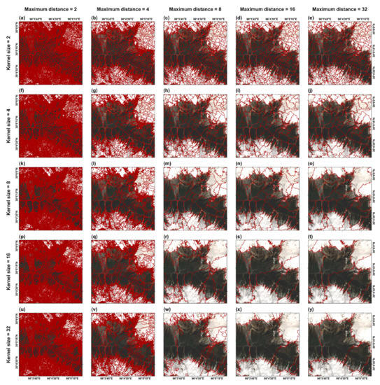
Figure 5.
Influence of different segmentation parameters in a subarea of the training zone. (Segmented objects are delineated in red polygons).
To further investigate the segmentation influence on the model performance, the samples built from different segmentations are used to train the RF models. Note that only features derived from the 10 multispectral bands are used and the models are only trained with the object samples that are within the training zone (i.e., the red box in Figure 2a). In this study, 100 decision trees are used in each RF model and the performance of the trained RF models is evaluated and listed in Table 3. Conditions of MD = 2 and 4 are not included in Table 3 due to excessive oversegmentation (Figure 5a,b,f,g,k,l,p,q,u,v). Referring to Table 2 and Table 3, it can be found that the segmentation loss has a negative correlation with the object number. Due to the segmentation loss, all the pixel-based indices are lower than the corresponding object-based indices under different conditions, and the pixel-based indices decrease as the segmentation loss increases. The best pixel-level mapping result is achieved by the segmentation using KZ = 2 and MD = 8, which has the object and pixel IoUs of 98.21% and 97.23%, respectively, and the object and pixel OA values of 98.76% and 98.07%, respectively. Although the pixel-based mapping performance decreases with increasing segmentation loss, the lowest pixel IoU and OA still reach 92.12% and 94.42%, respectively, proving the robustness of AutoSMILE.
Table 3.
Performance evaluation of snow mapping with different segmentation parameters using random forest (RF) over the study area in Bome County (excluding the training zone).
3.2. Snow Mapping Results of Different Datasets
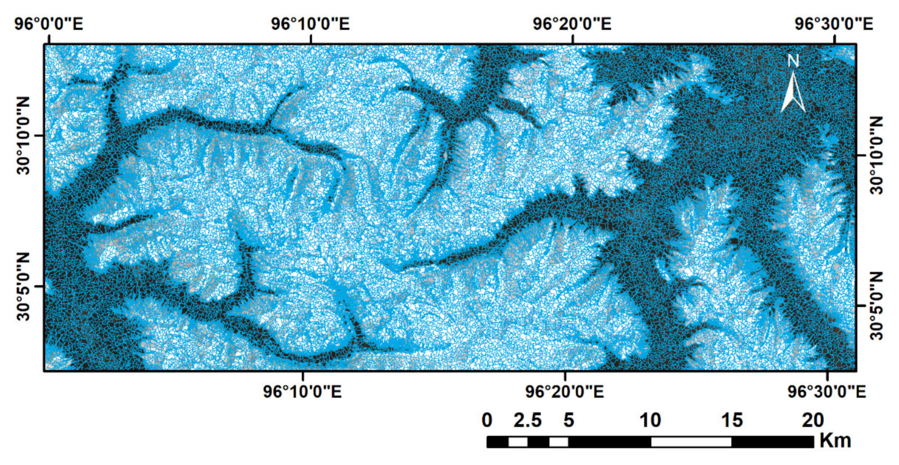
As suggested in Table 3, KZ = 2 and MD = 8 are adopted to conduct snow mapping. The segmentation of the study area is visualized in Figure 6. It can be seen that small objects concentrate in the transition zones between snow and non-snow land covers, and the objects inside the same land cover are larger and much sparser. There are 77,848 objects inside the study area. Among all the segmented objects, 3934 objects that are within the training zone are used for model training, and the rest of the objects are used for model testing.
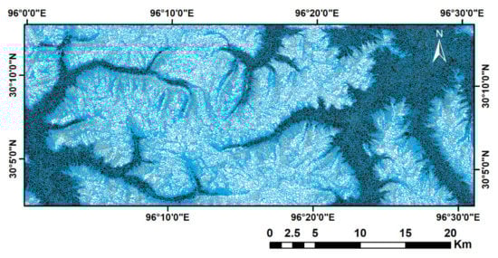
Figure 6.
Segmentation results using quickshift. (Kernel size = 2, maximum distance = 8, and segmented objects are delineated in blue polygons).
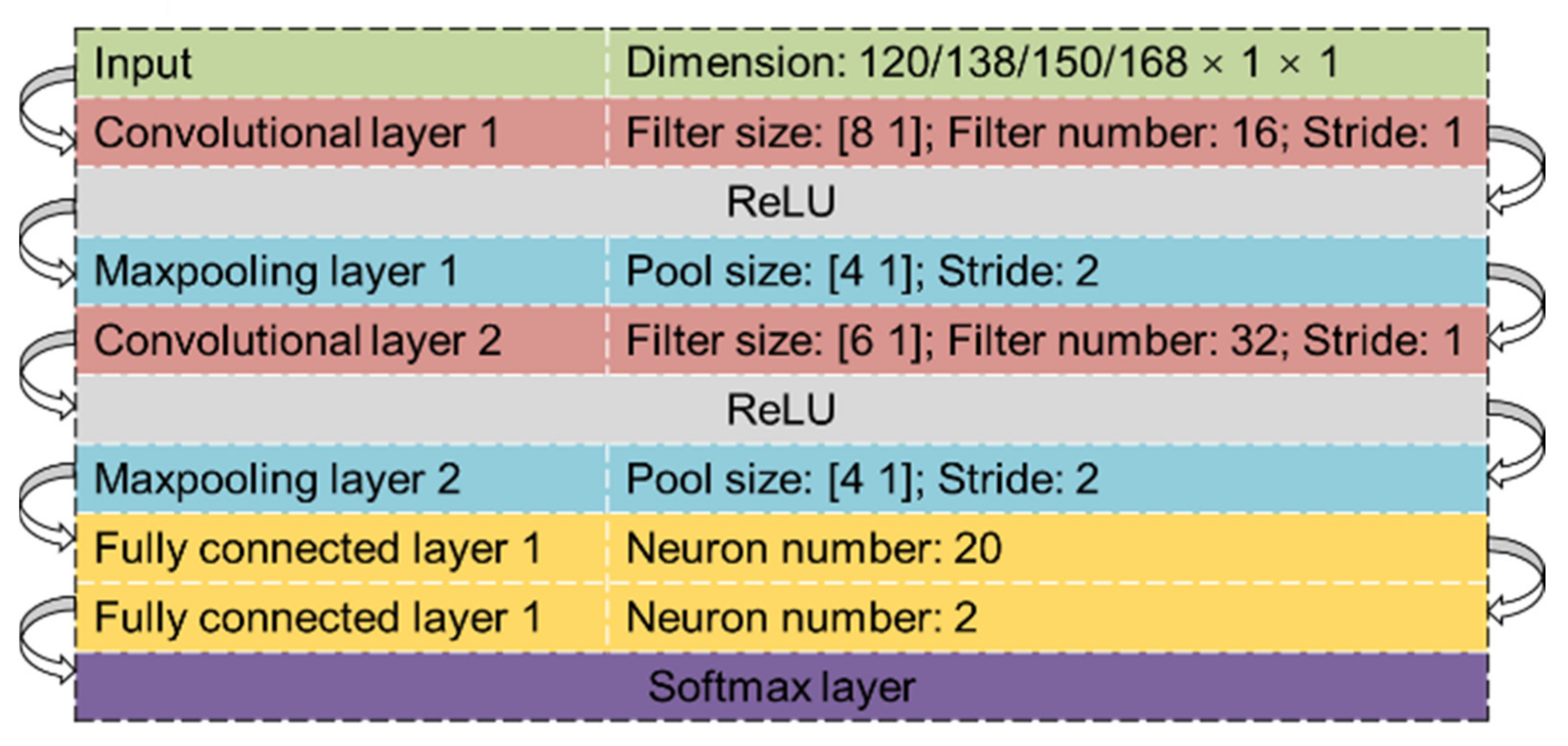
Based on the segmentation in Figure 6, snow maps with different dataset combinations were examined to assess the contributions from extra auxiliary data. Three datasets were created using features derived from different data layers; namely, multispectral image dataset (MSID), multispectral image derived dataset (MSIDD) and digital elevation model dataset (DEMD). MSID only uses the 10 spectral layers, which derive 60 band features and 60 texture features. MSIDD includes 18 features which are calculated based on derived NDVI, NDMI and MNDWI layers. DEMD consists of 30 features which are extracted from the DEM and its derivatives. Table 4 compares results of snow mapping using different dataset combinations, where both CNN and RF are applied. The structure of the CNN is presented in Figure 7. In this study, the Adam optimizer was used to train the CNN model. The learning rate, maximum number of epochs and the mini-batch size were set to 0.0003, 100 and 256, respectively. The machine learning models trained by different dataset combinations all performed extraordinarily well with only minor differences. Interestingly, in most cases, the RF models performed slightly better than the CNN models with an OA improvement of around 0.2% to 0.4%. Due to the low complexity of the datasets, it is reasonable that deep learning models do not necessarily outperform conventional models. Adding the MSIDD slightly increased the pixel PA of the CNN models (~0.14%) but the RF performed similarly in both cases. By contrast, adding the DEMD did not improve the snow mapping and even caused minor pixel OA losses of the RF (~0.15%) model. If both the MSIDD and DEMD were included, the performance difference was also negligible: the pixel OA of RF decreased 0.22%. Overall, the pixel IoU and OA of CNN was always stable regardless of any supplement of new features. With pixel IoUs ranging from 96.66% to 97.23% and pixel OAs ranging from 97.67% to 98.07%, it can be concluded that the performance of AutoSMILE is not sensitive to extra auxiliary data. The snow cover can be mapped with very high accuracy using only the multispectral image.
Table 4.
Performance evaluation of snow mapping with different datasets and machine learning algorithms over the study area (excluding the training zone).
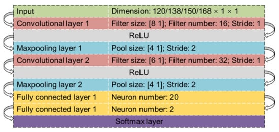
Figure 7.
Network architecture of the applied convolutional neural network model.
To understand how AutoSMILE performs across the entire study area, Figure 8 classifies each pixel into four groups (TP, TN, FP and FN) by taking different snow covers as ground truths and predictions. In Figure 8a, the spatial distribution of segmentation loss can be directly observed by taking the object-based snow cover as a prediction and the pixel-based snow cover as ground truth. It can be spotted that most FN pixels are distributed near the outer boundary of the snow area and most FP pixels spread over the gullies inside the snow area. Segmentation loss can hardly be eliminated in the object-based analysis as it is almost inevitable for some objects to have both snow and non-snow pixels after segmentation. The segmentation loss in this case is 1.17%, which is considered acceptable. Figure 8b shows the snow cover predicted by RF and MSID compared with the object-based snow cover. Although some objects are misclassified with RF, the overall snow area is complete, and the complex snow boundaries are successfully captured. Figure 8c compares the snow cover predicted by RF and MSID with the pixel-based snow cover. With less than 2% of misclassification pixels, the overall performance of AutoSMILE at pixel level is excellent. According to Figure 8, it is recommended that visual inspection of the final snow mapping product should focus more on the transition zones between snow and non-snow areas.
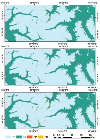
Figure 8.
Results of pixel classification using different snow covers as predictions and ground truths: (a) object-based snow cover as prediction and pixel-based snow cover as ground truth, (b) snow cover predicted by the random forest model as prediction and object-based snow cover as ground truth and (c) snow cover predicted by the random forest model as prediction and pixel-based snow cover as ground truth. (TP: true positive; TN: true negative; FP: false positive; and FN: false negative).
3.3. Layer Importance Analysis Based on the Best Model
To evaluate the contribution of different data layers in training the best model, a permutation-based feature importance analysis is conducted. By permuting the sample value of a specific feature, influential features could be identified if ML model performance drops. The importance of a layer is calculated as the average importance of the features derived from that layer. According to Table 4, the best ML model, which is trained with RF, MSID, KZ = 2 and MD = 8, is used to estimate the layer importance. Figure 9 shows the data layer importance relative to the red band layer, which is shown to be the most important to the model. However, the differences among the first three important layers (red, blue and green) are not significant. As these three bands can be integrated into the true-color image, it is not surprising that they rank at top. Texture layers rank the lowest, indicating that land cover in this study area is not sensitive to texture change.
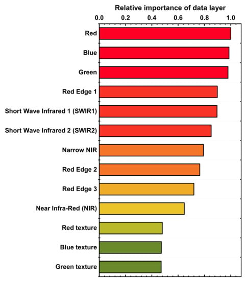
Figure 9.
Data layer importance relative to the red band layer.
4. Discussion
4.1. The Generalizability of the Trained AutoSMILE Model
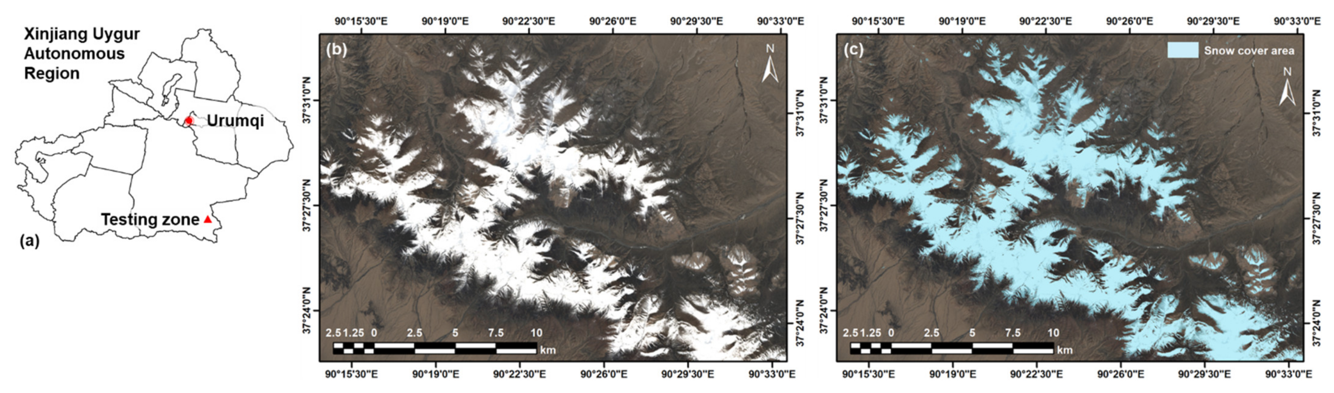
To assess the generalizability of the trained model in mapping snow covers for new images, a new multispectral image covering Qimantag Mountain in the western segment of eastern Kunlun Mountains, northern Tibetan Plateau, was acquired for extra testing. The image was captured by Sentinel 2B on 2 June 2019. In terms of administrative division, the new testing zone was at the southeast corner of the Xinjiang Uyghur Autonomous Region (Figure 10a). The true-color RGB image of the new testing zone is shown in Figure 10b, which covers an area of 579 km2. The manually interpreted snow cover is shown in Figure 10c. The ML models trained in Bome County were then directly applied to predict snow covers for the testing zone in the Qimantag Mountain region. Results are summarized in Table 5. Although the place, time and general environment changed, the RF model still achieves a pixel OA of 97.22% for the new testing zone, indicting a good generalizability of the ML model produced by AutoSMILE.
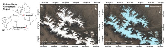
Figure 10.
(a) Location of the new testing zone; (b) true-color RGB image of the new testing zone and (c) pixel-level snow cover of the new testing zone based on visual interpretation.
Table 5.
Performance evaluation of snow mapping in the testing zone (Qimantag Mountain region).
4.2. Comparison of AutoSMILE and Threshold-Based Methods
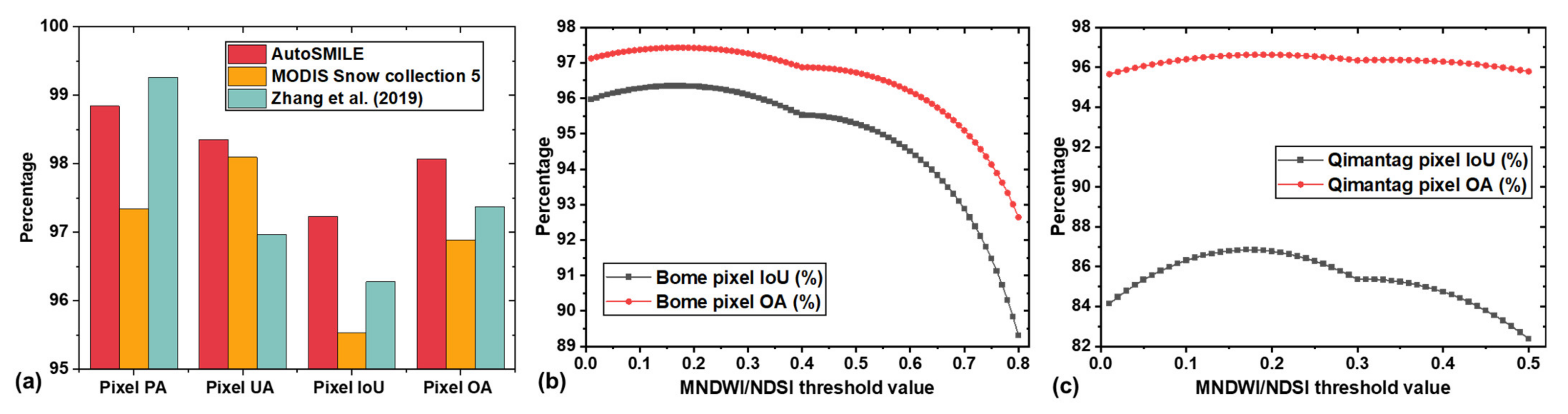
To further evaluate the performance of AutoSMILE, a comparative study between AutoSMILE and two existing threshold-based methods was conducted. The first threshold-based method was developed by NASA to produce the fifth version of MODIS Snow collection products, in which the following rules are applied: NDSI > 0.4, near-infrared reflectance (bandwidth: 841–876 nm) >0.11, and the band 4 reflectance (bandwidth: 545–565 nm) >0.1 [10]. The second method was proposed by Zhang et al. (2019), who found that a NDSI threshold of 0.1 is more reasonable than that of 0.4 for applications in China [6], so the second method simply applied the recommended threshold value (0.1) as the sole criterion. In Figure 11a, AutoSMILE (RF, KZ = 2, MD = 8, trained with MSID) ranks the first among the three methods in terms of the two most important indices: pixel IoU and OA. Compared with the MODIS method, AutoSMILE achieves a performance gain of 1.7% in terms of IoU and 1.2% in terms of OA, corresponding to a 11.4 km2 increase of correctly predicted area. When compared with the method of Zhang et al. (2019), the performance gains narrowed down to 1.0% of IoU and 0.7% of OA, corresponding to a 6.7 km2 increase of correctly predicted area. In order to find the optimal threshold value for both study areas, we further adopted the third method: testing all the NDSI values ranging from 0.01 to 0.80. The result of the study area in Bome County is shown in Figure 11b. It was found that the optimal threshold was 0.17 that gave an IoU of 96.35% and an OA of 97.43%. When examining the testing zone in the Qimantag Mountain region, the optimal threshold turned out to be 0.19, which gave an IoU of 86.81% and an OA of 96.63%. The changing optimal thresholds indicated that the threshold-based method could hardly find a universally applicable threshold. It usually required a site-specific calibration in order to obtain the best performance. In addition, in the Qimantag Mountain region, the RF model trained in Bome County outperformed the threshold-based method by 2.3% and 0.6% in terms of pixel IoU and OA, respectively.

Figure 11.
Results of the comparative study: (a) performance of different methods over the study area in Bome County (excluding the training zone); (b) performance of MNDWI/NDSI-based method as functions of threshold value over the study area in Bome County (excluding the training zone); (c) performance of MNDWI/NDSI-based method as functions of threshold value over the new testing zone in the Qimantag Mountain region. (PA: producer’s accuracy; UA: user’s accuracy; IoU: intersection over union; OA: overall accuracy; MNDWI: modified normalized difference water index; and NDSI: normalized difference snow index).
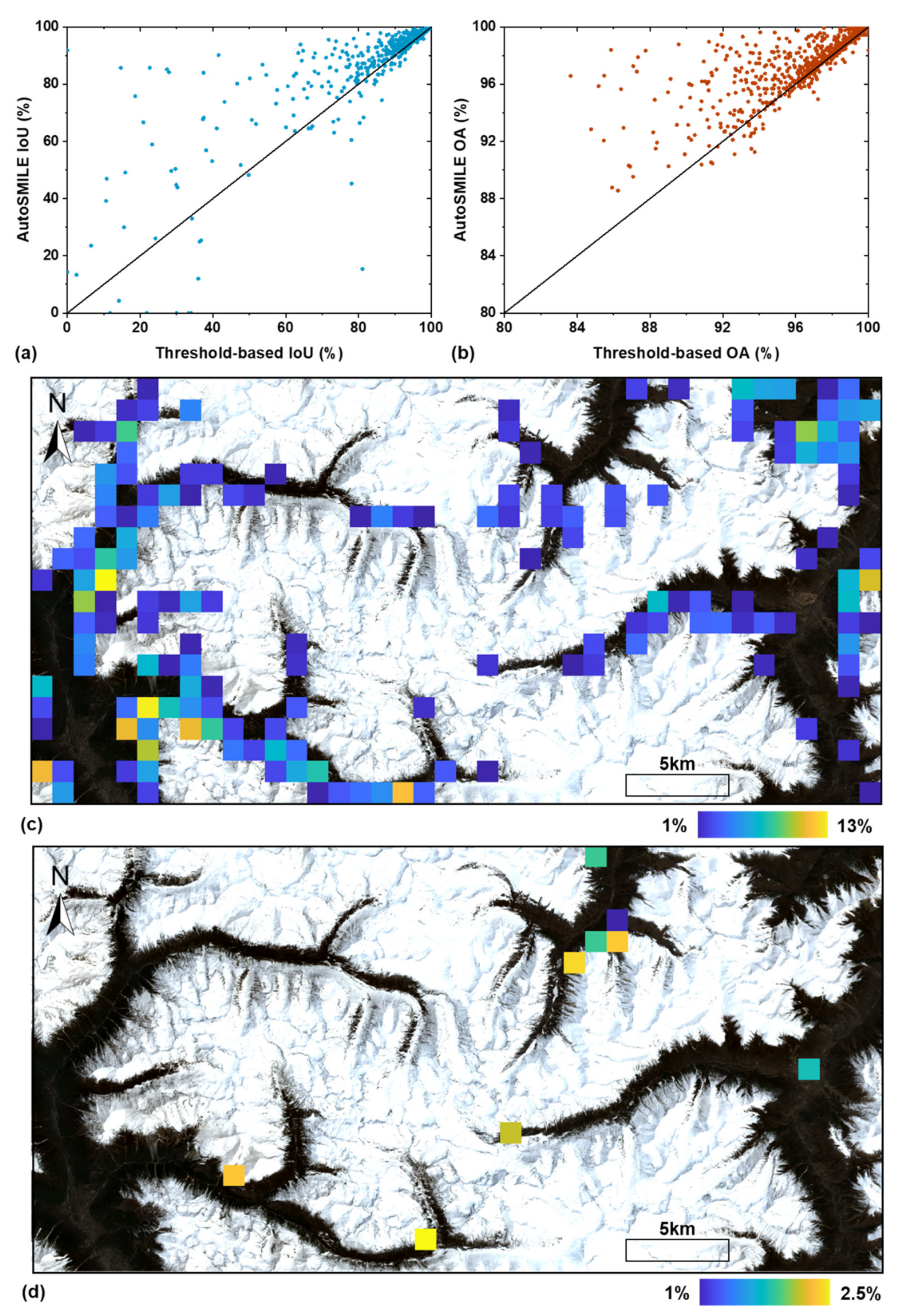
A more detailed comparison is presented in Figure 12 to illustrate how different methods perform at sub-regions of the study area in Bome County. The whole study area was first discretized into tiles of 1 × 1 km2. As our study area occupied 20.12 × 49.79 km2, in total 980 tiles were created and some marginal southern and eastern areas were omitted. Then, inside each tile, pixel-based IoU and OA were calculated based on the AutoSMILE method and the best threshold method at the study area in Bome County (NDSI > 0.17), respectively. IoU and OA results are shown in Figure 12a,b. It can be seen that vast majority of the data points concentrate either above or near the 1:1 line, indicating that the threshold-based method barely outperforms AutoSMILE in the sub-regions. A maximum increase of 92% of IoU can be observed in Figure 12a. Figure 12c further shows the spatial distribution of tiles where AutoSMILE-based OA (OAAutoSMILE) exceeds the threshold-based OA (OAthreshold) by at least 1%. Most identified tiles are located in the transition zones, and the highest OA difference reaches about 13%, indicating that AutoSMILE is particularly good at handling complex land cover conditions. Figure 12d presents the tiles where OAthreshold − OAAutoSMILE >1%. It can be noticed that very limited tiles fulfill this condition, and the highest OA difference is only around 2.5%. Combining Figure 12c,d, it can be concluded that both methods perform quite well inside the same land cover; however, when encountering complex land covers like the transition zones, AutoSMILE outperforms the threshold-based method substantially.
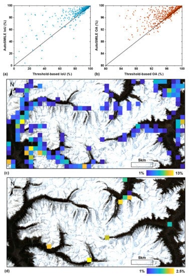
Figure 12.
Comparison results between AutoSMILE and the best threshold-based method (NDSI > 0.17) in the study area of Bome County: (a) scatter plot of IoUs of 1 × 1 km2 tiles using the two methods; (b) scatter plot of OAs of 1 × 1 km2 tiles using the two methods; (c) OA difference heatmap of 1 × 1 km2 tiles where OAAutoSMILE − OAthreshold > 1% and (d) OA difference heatmap of 1 × 1 km2 tiles where OAthreshold − OAAutoSMILE > 1%. (NDSI means the normalized difference snow index, IoU means the intersection over union, and OA means the overall accuracy).
5. Conclusions
An automated snow mapper powered by machine learning, AutoSMILE, which is the first machine learning-based open-source system for snow mapping, was developed and tested in two regions on the Tibetan Plateau. The first region was taken as the main study area (Bome County, 1102 km2) and the second region was only used for model testing (Qimantag Mountain region, 579 km2). The machine learning techniques and object-based analysis were successfully integrated for snow mapping in the two regions. The following conclusions can be drawn:
- Using only 5% of the main study area for training (50.4 km2), AutoSMILE achieves extraordinarily satisfactory results of snow mapping in the rest of the main study area: object and pixel PAs, UAs, IoUs and OA values reaching 99.42% and 98.78%, 98.21% and 98.76%, 98.84% and 98.35%, and 97.23% and 98.07%, respectively. When applying the trained models to the testing zone in Qimantag Mountain region, the highest OA reaches 97.22%, indicating the excellent performance, generalizability and robustness of AutoSMILE.
- According to the parametric study of segmentation parameters, KZ and MD should be carefully determined. In AutoSMILE, a low MD is not recommended to avoid excessive oversegmentation and low computational efficiency, but a small value of KZ is recommended to better handle the transition zone between snow and non-snow areas.
- Results of alternating dataset combinations indicate that auxiliary data like multispectral image derived indices and DEM derivatives play a limited role in enhancing the performance of AutoSMILE. High-quality snow mapping can be accomplished with only the multispectral image using AutoSMILE. Based on permutation importance analysis of the best ML model, the top five important layers are red, blue, green, red edge 1 and short wave infrared 1 band layers.
- AutoSMILE outperforms the existing threshold-based methods in both regions. The optimal NDSI thresholds of the two regions vary, suggesting that the threshold method typically requires site knowledge to achieve the best performance and it is hard to find a universally applicable threshold. When investigating the performance at the sub-regions, it was found that both AutoSMILE and threshold-based methods perform well when the land cover is simple. However, when encountering complex conditions like snow mapping in transition zones, AutoSMILE outperforms the threshold-based method substantially (up to 92% of IoU increase and up to 13% of OA increase).
- Due to the inevitable segmentation loss induced by object-based analysis, transition zones between snow and non-snow areas require more attention when inspecting the final snow cover products.
Author Contributions
Conceptualization, H.W. and L.Z.; methodology, formal analysis, data curation, H.W. and L.W.; software, validation, investigation, H.W., J.H. and H.L.; writing—original draft preparation, H.W.; writing—review and editing, supervision, project administration, funding acquisition, L.Z. All authors have read and agreed to the published version of the manuscript.
Funding
This research is supported by NSFC/RGC Joint Research Scheme (No. N_HKUST620/20), the National Natural Science Foundation of China (No. U20A20112), and the Research Grants Council of the Hong Kong SAR Government (Nos. 16203720 and 16205719).
Data Availability Statement
The Sentinel-2 multispectral products in this study are available at Copernicus Open Access Hub of ESA (https://scihub.copernicus.eu/, accessed on 30 September 2021) and the DEM data are download from the ASF DAAC (https://search.asf.alaska.edu/, accessed on 30 September 2021).
Acknowledgments
The authors would like to thank ESA and ASF DAAC for providing the necessary data for this study.
Conflicts of Interest
The authors declare no conflict of interest.
References
- Arino, O.; Bicheron, P.; Achard, F.; Latham, J.; Witt, R.; Weber, J.L. The Most Detailed Portrait of Earth. Eur. Space Agency 2008, 136, 25–31. [Google Scholar]
- Dedieu, J.-P.; Carlson, B.Z.; Bigot, S.; Sirguey, P.; Vionnet, V.; Choler, P. On the Importance of High-Resolution Time Series of Optical Imagery for Quantifying the Effects of Snow Cover Duration on Alpine Plant Habitat. Remote Sens. 2016, 8, 481. [Google Scholar] [CrossRef] [Green Version]
- Biemans, H.; Siderius, C.; Lutz, A.F.; Nepal, S.; Ahmad, B.; Hassan, T.; von Bloh, W.; Wijngaard, R.R.; Wester, P.; Shrestha, A.B.; et al. Importance of Snow and Glacier Meltwater for Agriculture on the Indo-Gangetic Plain. Nat. Sustain. 2019, 2, 594–601. [Google Scholar] [CrossRef]
- Croce, P.; Formichi, P.; Landi, F.; Mercogliano, P.; Bucchignani, E.; Dosio, A.; Dimova, S. The Snow Load in Europe and the Climate Change. Clim. Risk Manag. 2018, 20, 138–154. [Google Scholar] [CrossRef]
- Zhao, J.; Shi, Y.; Huang, Y.; Fu, J. Uncertainties of Snow Cover Extraction Caused by the Nature of Topography and Underlying Surface. J. Arid Land 2015, 7, 285–295. [Google Scholar] [CrossRef]
- Zhang, H.; Zhang, F.; Zhang, G.; Che, T.; Yan, W.; Ye, M.; Ma, N. Ground-Based Evaluation of MODIS Snow Cover Product V6 across China: Implications for the Selection of NDSI Threshold. Sci. Total Environ. 2019, 651, 2712–2726. [Google Scholar] [CrossRef]
- Härer, S.; Bernhardt, M.; Siebers, M.; Schulz, K. On the Need for a Time- and Location-Dependent Estimation of the NDSI Threshold Value for Reducing Existing Uncertainties in Snow Cover Maps at Different Scales. Cryosphere 2018, 12, 1629–1642. [Google Scholar] [CrossRef]
- Hall, D.K.; Riggs, G.A.; Salomonson, V.V.; Barton, J.; Casey, K.; Chien, J.; DiGirolamo, N.; Klein, A.; Powell, H.; Tait, A. Algorithm Theoretical Basis Document (ATBD) for the MODIS Snow and Sea Ice-Mapping Algorithms; NASA Goddard Space Flight Center: Greenbelt, MD, USA, 2001. [Google Scholar]
- Gascoin, S.; Grizonnet, M.; Bouchet, M.; Salgues, G.; Hagolle, O. Theia Snow Collection: High-Resolution Operational Snow Cover Maps from Sentinel-2 and Landsat-8 Data. Earth Syst. Sci. Data 2019, 11, 493–514. [Google Scholar] [CrossRef] [Green Version]
- Hall, D.K.; Salomonson, V.V. MODIS Snow Products User Guide to Collection 5; NASA Goddard Space Flight Center: Greenbelt, MD, USA, 2006. [Google Scholar]
- Hall, D.K.; Riggs, G.A. Accuracy Assessment of the MODIS Snow Products. Hydrol. Process. 2007, 21, 1534–1547. [Google Scholar] [CrossRef]
- Stumpf, A.; Kerle, N. Object-Oriented Mapping of Landslides Using Random Forests. Remote Sens. Environ. 2011, 115, 2564–2577. [Google Scholar] [CrossRef]
- Ghorbanzadeh, O.; Blaschke, T.; Gholamnia, K.; Meena, S.R.; Tiede, D.; Aryal, J. Evaluation of Different Machine Learning Methods and Deep-Learning Convolutional Neural Networks for Landslide Detection. Remote Sens. 2019, 11, 196. [Google Scholar] [CrossRef] [Green Version]
- Keyport, R.N.; Oommen, T.; Martha, T.R.; Sajinkumar, K.S.; Gierke, J.S. A Comparative Analysis of Pixel- and Object-Based Detection of Landslides from Very High-Resolution Images. Int. J. Appl. Earth Obs. Geoinf. 2018, 64, 1–11. [Google Scholar] [CrossRef]
- Rastner, P.; Bolch, T.; Notarnicola, C.; Paul, F. A Comparison of Pixel- and Object-Based Glacier Classification with Optical Satellite Images. IEEE J. Sel. Top. Appl. Earth Obs. Remote Sens. 2014, 7, 853–862. [Google Scholar] [CrossRef]
- Wang, X.; Gao, X.; Zhang, X.; Wang, W.; Yang, F. An Automated Method for Surface Ice/Snow Mapping Based on Objects and Pixels from Landsat Imagery in a Mountainous Region. Remote Sens. 2020, 12, 485. [Google Scholar] [CrossRef] [Green Version]
- Wang, H.J.; Zhang, L.M.; Xiao, T. DTM and Rainfall-Based Landslide Susceptibility Analysis Using Machine Learning: A Case Study of Lantau Island, Hong Kong. In Proceedings of the The Seventh Asian-Pacific Symposium on Structural Reliability and Its Applications (APSSRA 2020), Tokyo, Japan, 4–7 October 2020. [Google Scholar]
- Wang, H.J.; Xiao, T.; Li, X.Y.; Zhang, L.L.; Zhang, L.M. A Novel Physically-Based Model for Updating Landslide Susceptibility. Eng. Geol. 2019, 251, 71–80. [Google Scholar] [CrossRef]
- Rastegarmanesh, A.; Moosavi, M.; Kalhor, A. A Data-Driven Fuzzy Model for Prediction of Rockburst. Georisk Assess. Manag. Risk Eng. Syst. Geohazards 2021, 15, 152–164. [Google Scholar] [CrossRef]
- Hosseini, S.A.A.; Mojtahedi, S.F.F.; Sadeghi, H. Optimisation of Deep Mixing Technique by Artificial Neural Network Based on Laboratory and Field Experiments. Georisk Assess. Manag. Risk Eng. Syst. Geohazards 2020, 14, 142–157. [Google Scholar] [CrossRef]
- Wang, L.; Chen, Y.; Tang, L.; Fan, R.; Yao, Y. Object-Based Convolutional Neural Networks for Cloud and Snow Detection in High-Resolution Multispectral Imagers. Water 2018, 10, 1666. [Google Scholar] [CrossRef] [Green Version]
- Liu, C.; Huang, X.; Li, X.; Liang, T. MODIS Fractional Snow Cover Mapping Using Machine Learning Technology in a Mountainous Area. Remote Sens. 2020, 12, 962. [Google Scholar] [CrossRef] [Green Version]
- Rahmati, O.; Ghorbanzadeh, O.; Teimurian, T.; Mohammadi, F.; Tiefenbacher, J.P.; Falah, F.; Pirasteh, S.; Ngo, P.T.T.; Bui, D.T. Spatial Modeling of Snow Avalanche Using Machine Learning Models and Geo-Environmental Factors: Comparison of Effectiveness in Two Mountain Regions. Remote Sens. 2019, 11, 2995. [Google Scholar] [CrossRef] [Green Version]
- Tsai, Y.-L.S.; Dietz, A.; Oppelt, N.; Kuenzer, C. Wet and Dry Snow Detection Using Sentinel-1 SAR Data for Mountainous Areas with a Machine Learning Technique. Remote Sens. 2019, 11, 895. [Google Scholar] [CrossRef] [Green Version]
- Cannistra, A.F.; Shean, D.E.; Cristea, N.C. High-Resolution Cubesat Imagery and Machine Learning for Detailed Snow-Covered Area. Remote Sens. Environ. 2021, 258, 112399. [Google Scholar] [CrossRef]
- Liu, Y.; Chen, X.; Hao, J.-S.; Li, L.-H. Snow Cover Estimation from MODIS and Sentinel-1 SAR Data Using Machine Learning Algorithms in the Western Part of the Tianshan Mountains. J. Mt. Sci. 2020, 17, 884–897. [Google Scholar] [CrossRef]
- Brodu, N. Super-Resolving Multiresolution Images with Band-Independent Geometry of Multispectral Pixels. IEEE Trans. Geosci. Remote Sens. 2017, 55, 4610–4617. [Google Scholar] [CrossRef] [Green Version]
- Moore, I.D.; Grayson, R.B.; Ladson, A.R. Digital Terrain Modelling: A Review of Hydrological, Geomorphological, and Biological Applications. Hydrol. Process. 1991, 5, 3–30. [Google Scholar] [CrossRef]
- Wilson, E.H.; Sader, S.A. Detection of Forest Harvest Type Using Multiple Dates of Landsat TM Imagery. Remote Sens. Environ. 2002, 80, 385–396. [Google Scholar] [CrossRef]
- Xu, H.Q. Modification of Normalised Difference Water Index (NDWI) to Enhance Open Water Features in Remotely Sensed Imagery. Int. J. Remote Sens. 2006, 27, 3025–3033. [Google Scholar] [CrossRef]
- Vedaldi, A.; Soatto, S. Quick Shift and Kernel Methods for Mode Seeking. In Computer Vision—ECCV 2008, Proceedings of the European Conference on Computer Vision, Marseille, France, 23–28 August 2008; Springer: Berlin/Heidelberg, Germany, 2008; pp. 705–718. [Google Scholar]
- Haralick, R.M. Statistical and Structural Approaches to Texture. Proc. IEEE 1979, 67, 786–804. [Google Scholar] [CrossRef]
- Wang, H.; Zhang, L.; Yin, K.; Luo, H.; Li, J. Landslide Identification Using Machine Learning. Geosci. Front. 2021, 12, 351–364. [Google Scholar] [CrossRef]
- Wang, H.J.; Zhang, L.M.; Luo, H.Y.; He, J.; Cheung, R.W.M. AI-Powered Landslide Susceptibility Assessment in Hong Kong. Eng. Geol. 2021, 288, 106103. [Google Scholar] [CrossRef]
- James, G.; Witten, D.; Hastie, T.; Tibshirani, R. An Introduction to Statistical Learning; Springer: New York, NY, USA, 2013. [Google Scholar]
- Goodfellow, I.; Bengio, Y.; Courville, A. Deep Learning; MIT Press: London, UK, 2016. [Google Scholar]


Publisher’s Note: MDPI stays neutral with regard to jurisdictional claims in published maps and institutional affiliations. |
© 2021 by the authors. Licensee MDPI, Basel, Switzerland. This article is an open access article distributed under the terms and conditions of the Creative Commons Attribution (CC BY) license (https://creativecommons.org/licenses/by/4.0/).