Article

Ground Observations and Environmental Covariates Integration for Mapping of Soil Salinity: A Machine Learning-Based Approach

by
Salman Naimi
1,
Shamsollah Ayoubi
1,
Mojtaba Zeraatpisheh
2,3,* and
Jose Alexandre Melo Dematte
4
1
Department of Soil Science, College of Agriculture, Isfahan University of Technology, Isfahan 841156-83111, Iran
2
Henan Key Laboratory of Earth System Observation and Modeling, Henan University, Kaifeng 475004, China
3
College of Geography and Environmental Science, Henan University, Kaifeng 475004, China
4
Department of Soil Science, Luiz de Queiroz College of Agriculture, Av. Pádua Dias, 11, Piracicaba 13418-900, SP, Brazil
*
Author to whom correspondence should be addressed.
Remote Sens. 2021, 13(23), 4825; https://doi.org/10.3390/rs13234825
Submission received: 14 October 2021 / Revised: 22 November 2021 / Accepted: 24 November 2021 / Published: 27 November 2021
(This article belongs to the Special Issue Advances of Proximal and Remote Sensing in Soil Salinity Mapping)

Abstract

:
Soil salinization is a severe danger to agricultural activity in arid and semi-arid areas, reducing crop production and contributing to land destruction. This investigation aimed to utilize machine learning algorithms to predict spatial soil salinity (dS m−1) by combining environmental covariates derived from remotely sensed (RS) data, a digital elevation model (DEM), and proximal sensing (PS). The study is located in an arid region, southern Iran (52°51′–53°02′E; 28°16′–28°29′N), in which we collected 300 surface soil samples and acquired the spectral data with RS (Sentinel-2) and PS (electromagnetic induction instrument (EMI) and portable X-ray fluorescence (pXRF)). Afterward, we analyzed the data using five machine learning methods as follows: random forest—RF, k-nearest neighbors—kNN, support vector machines—SVM, partial least squares regression—PLSR, artificial neural networks—ANN, and the ensemble of individual models. To estimate the electrical conductivity of the saturated paste extract (ECe), we built three scenarios, including Scenario (1): Synthetic Soil Image (SySI) bands and salinity indices derived from it; Scenario (2): RS data, PS data, topographic attributes, and geology and geomorphology maps; and Scenario (3): the combination of Scenarios (1) and (2). The best prediction accuracy was obtained for the RF model in Scenario (3) (R2 = 0.48 and RMSE = 2.49), followed by Scenario (2) (RF model, R2 = 0.47 and RMSE = 2.50) and Scenario (1) for the SVM model (R2 = 0.26 and RMSE = 2.97). According to ensemble modeling, a combined strategy with the five models exceeded the performance of all the single ones and predicted soil salinity in all scenarios. The results revealed that the ensemble modeling method had higher reliability and more accurate predictive soil salinity than the individual approach. Relative improvement (RI%) showed that the R2 index in the ensemble model improved compared to the most precise prediction for the Scenarios (1), (2), and (3) with 120.95%, 56.82%, and 66.71%, respectively. We applied the best model in each scenario for mapping the soil salinity in the selected area, which indicated that ECe tended to increase from the northwestern to south and southeastern regions. The area with high ECe was located in the regions that mainly had low elevations and playa. The areas with low ECe were located in the higher elevations with steeper slopes and alluvial fans, and thus, relief had great importance. This study provides a precise, cost-effective, and scientific base prediction for decision-making purposes to map soil salinity in arid regions.

Graphical Abstract

1. Introduction

As one of the most common environmental concerns, soil salinization is a severe threat to agricultural activity in arid and semi-arid districts, reducing crop production and contributing to land destruction [1]. In these areas, lands that are widely irrigated, mainly to improve water use efficiency, the irrigation system has been changed from flood to drip irrigation, which has caused the accumulation of salts in the root zone and surface soil salinization [2]. In the last decades, Iran has faced increasing soil salinization problems due to increasing drought because of climate change consequences and human pressures on land and water resources in this region [3]. Therefore, accurate and reliable salinity mapping is needed to monitor and assess saline soil and manage the issue [4]. However, due to the high spatio-temporal variability in soil salinity, a timely and accurate approach is essential for soil salinity prediction to prevent and control soil degradation and ecological restoration in arid and semi-arid districts [5].
Traditional soil mapping is laborious, expensive, and not suitable to cover extended areas [6]. Using the digital soil mapping (DSM) technique can solve the problems of traditional methods and is a practical alternative [7,8,9,10]. Currently, several environmental covariates, including topographic ones, legacy soil maps, and remote sensing (RS) and proximal sensing (PS) data, were applied as auxiliary covariates for predicting soil properties, including soil salinity [4,5], soil organic carbon [11], and soil classes [12] for DSM technique.
McBratney et al. [7] explicated several modeling methods used in DSM investigations. Machine learning algorithms have been extensively applied in DSM to achieve the relationships between the spatial variation of soil characteristics and environmental covariates and then derive the spatial variability of soil attributes. This method is more successful at evaluating non-linear interactions between soil and environmental covariates [13]. Many machine learning algorithms have been assessed for soil properties prediction, including Cubist [14,15], artificial neural networks [16,17], partial least squares regression [18,19], k-nearest neighbors [19], regression kriging [20,21], multinomial logistic regression [12], multiple linear regression [22], random forests [23,24], random forest regression [25], support vector machines [17,26], and genetic algorithms [16].
RS data from satellite images, i.e., the Sentinel-2 Multi-Spectral Instrument (S2-MSI), are commonly used to investigate the spatial variation of soil salinity in agricultural regions and other land resources [27,28,29,30,31]. Meanwhile, PS data are increasingly being utilized to map soils with high spatial resolution in order to support precision agriculture and land management [32,33]. This data comprises measuring soil properties with geophysical field and laboratory sensors in order to directly or indirectly forecast and map soil properties of interest.
Electromagnetic induction instrument (EMI) sensors and portable X-ray fluorescence spectrometry (pXRF) are used to quantify soil properties in situ or in the laboratory. Several researchers have considered apparent electrical conductivity (ECa) as a convenient source of ancillary information for mapping soil salinity [4,34,35,36,37]. Additionally, other scholars have used data obtained from pXRF for predicting and mapping soil properties [38,39,40,41]. It seems that among the available environmental covariates for mapping soil salinity, the RS and PS techniques using the EMI and pXRF spectrometry have been of significant importance because they are good instruments for prediction, temporal monitoring, and mapping of soil salinity in conjunction with field measurements. However, there is little attempt to combine these two datasets for predicting soil properties, especially soil salinity in arid lands.
In recent years, in most arid and semi-arid regions in Iran, soluble salts have accumulated in the soil surface. The main reasons for this phenomenon are low precipitation and human activities, such as irrigation with saline water (low-quality water), improper water and soil management, overexploitation of groundwater, and insufficient drainage. Moreover, due to a lack of information about the spatial variability of soil salinity, land use planning was conducted inappropriately by decision-makers. As a result, the production of agricultural products has been gradually decreased. Therefore, to manage this problem, regular monitoring of soil salinity and detailed knowledge regarding its spatial distribution is essential [42].
As mentioned, there is little attempt to combine RS data and auxiliary environmental data with PS data to predict soil salinity. Since soil sensing is range-specific with attributes, soil attributes could thus be defined in different spectral ranges. This study expects that PS detects the salinity elements and remotely assists in specialization using the machine learning system. As a result, the main goals of this study were (i) to predict soil salinity spatially by combining RS data and environmental covariates with PS such as EMI and pXRF, (ii) evaluate the capability of different machine learning methods including PLSR, SVM, RF, ANN, kNN, and the ensemble of individual models for predicting soil salinity, and (iii) to determine the most important covariates for predicting soil salinity by sensitivity analysis in an arid region, southern Iran.

2. Materials and Methods

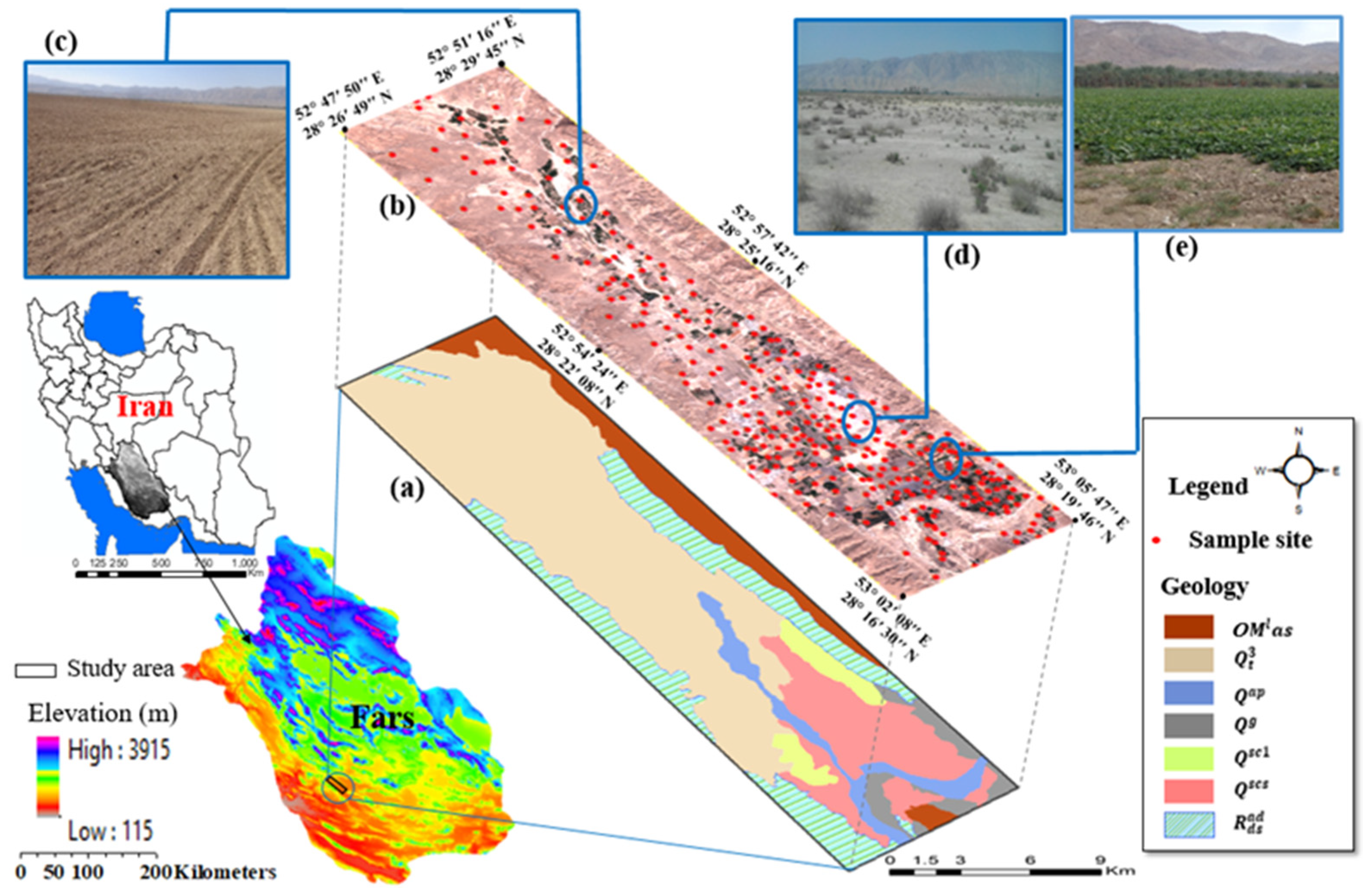
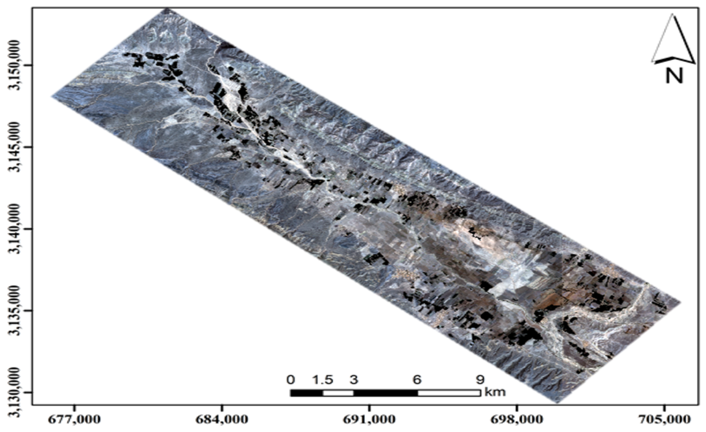
2.1. Description of the Study Area

The study site is located at the Afzar region in Fars province (part of the folded Zagros) south of Iran (52°51′–53°02′E; 28°16′–28°29′N) and covers 242 km2. Most of the study area is almost flat with a slope of 1–4%, and the elevation varies from 597 to 723 m above sea level (Figure 1). The predominant crops cultivated in the plain included citrus and dates, followed by wheat, barley, maize, and cucurbits. In the study area, the climate is the hot desert climate (BWh in the Köppen–Geiger classification) with a mean annual temperature and precipitation of 22.8 °C and 240 mm, respectively [43]. The precipitation mainly occurs during the cold months (November to March), and the local temperature ranges from −3 °C in January to 43.4 °C in July. The average annual evaporation is 2900 to 3400 mm [44]. The study area comprises various geological units, including deposits consisting of alluvial deposits, limestone, shale, and marl [45] (Figure 1a). The soils of the northern parts of the region are mainly from silty, sand, and clay flats ( Q t 3 ) and the soils of the southern parts are from flood plain deposits consisting of silt, clay, and sand with salt ( Q s c s ) and marsh deposits consisting of silt and clay with salt ( Q s c 1 ) (Figure 1a). The cultivated lands in the northern areas are irrigated with quality water, while the irrigated lands in the southern areas are irrigated with saline water, and this has probably caused the salinization of the soils in these areas. The study area comprises several landforms, including alluvial fans, bajada, alluvial plains, pediment, and clay flats (playa) (Figure 2 and Table 1). The major geoformation processes, especially in the late Tertiary and early Quaternary periods, are erosional and depositional processes. According to Soil Taxonomy, the soil temperature and moisture regimes are Hyperthermic and Aridic-Ustic, respectively. Moreover, soils in this region are predominantly classified under three sub-great groups: Ustic Haplocalcids, Ustic Haplocambids, and Ustic Torriorthents [46].

2.2. Data Collection and Soil Sample Analyses

A total of 300 surface soil samples (0–30 cm) were collected using the conditional Latin hypercube sampling (cLHS) technique [47], which was based on a wide variety of environmental covariates (RS indices, topographic attributes, geology and geomorphology maps) (Figure 1). The soil samples were prepared based on the standard method, and the electrical conductivity of the saturated paste extract (ECe) was determined using a conductivity meter [48,49].
The electromagnetic induction device (EMI, Geonics EM38) was used to determine the ECa at the sampled locations. The instrument is capable of measuring ECa in two modes: horizontal (ECah) and vertical (ECav), with effective depths of 0.75 and 1.5 m, respectively [50]. The EMI readings were performed in July 2019, when soil moisture was minimal, to minimize the soil moisture variation effects. Although diurnal temperature variation has little effect on ECa [51], the measurements were taken midmorning to coincide with soil surface that might be a daily average temperature.
Moreover, the elemental concentrations of the dry-sifted samples were determined using pXRF equipment [38]. The instrument was operated in Soil Mode, which is capable of detecting various elements. Scanning for Soil Mode was performed at a rate of 30 s per beam. Each sample was scanned once in Soil Mode; however, each scan was an average of internal scans performed at 1 s intervals. The pXRF output generated a geochemical profile of elemental concentrations and raw pXRF spectra for each of the three beams. Considering both the precision level of the XRF and the elemental ranges of the samples used in Soil Mode, only the contents of four elements (K: potassium; Ca: calcium; S: sulfur; Cl: chlorine) were used in this study because these elements are the main constituents of soluble salts in soil (e.g., various combinations of Mg2+, Na+, K+, Ca2+, Cl, SO42−, CO32−, and HCO3) [52].

2.3. Collection of Auxiliary Data

The environmental covariates employed in this study included four auxiliary covariates comprising RS indices, PS data, topographic covariates taken from a digital elevation model (DEM), and geology and geomorphology maps (Table 2).

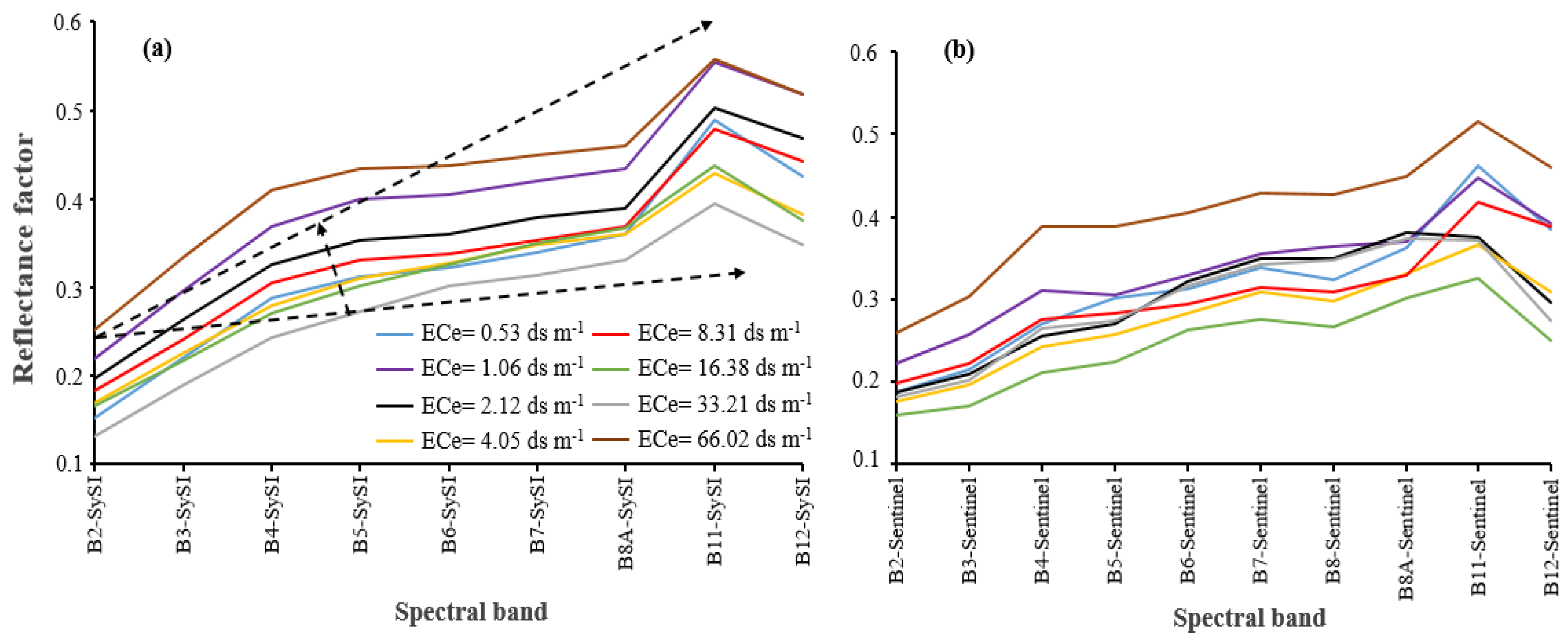
2.3.1. Remote Sensing and Selection of Spectral Index

The RS image data used in this investigation were derived from Sentinel-2A. The satellite images in this study were obtained from the website [62] (https://scihub.copernicus.eu/dhus/#/home, accessed on 23 November 2021) of the European Space Agency [63] (https://www.esa.int/ESA, accessed on 23 November 2021), which was basically synchronous with the sampling time, and there was no cloud in the study area. Furthermore, we used the multi-temporal bare soil technique from the Sentinel-2A satellite. Multi-temporal bare soil images known as SySI (Synthetic Soil Image) were produced from the Sentinel-2A images using the Geospatial Soil Sensing System method (GEOS3) [64]. Images from the Sentinel-2A satellite, at Level-1C (Top of Atmosphere reflectance, TOA), were obtained from the Copernicus website [62] (https://scihub.copernicus.eu/dhus/#/home, accessed on 23 November 2021), from 2015 to 2020. These needed to be corrected from TOA to BOA (Bottom of Atmosphere); thus, we used the Sen2Cor plugin for correction [65]. These Level-2A (BOA) images were processed using the statistical software R [66]. Sentinel-2 MSI images have a spatial resolution of 10 to 60 m, but we used spectral bands with 10 and 20 m pixel sizes. The near-infrared (NIR) bands (band 8A) were available in 10 m pixel size and were resampled to 20 m using the resample function and the bilinear method in R software to ensure the same spatial extent of all spectral bands [66].
The GEOS3 method consists of (1) obtaining the images, (2) masking pixels that were non-bare soil, and (3) calculating the median reflectance of the masked images. After obtaining the images, spectral indices such as NBR2 (Normalized Burn Ratio 2) and NDVI (Normalized Difference Vegetation Index) were calculated and used to mask the images. Following the GEOS3 method, each of the images obtained was masked from two spectral indices. The NDVI was used to mask vegetation (Equation (1)), both natural and planted. For this purpose, all pixels that were not in the range of −0.15 to 0.25 were discarded, maintaining only those that had a soil response. Then NBR2 was used to mask straw (Equation (2)), with an interval between −0.15 and 0.15. Subsequently, cloud or cloud shadow was also masked to prevent them from interfering with the final image. Then, using the median between the pixels of all satellite images, SySI was calculated. The SySI was composed of nine surface reflectance data from the regions visible, near-infrared, and shortwave infrared (Vis-NIR-SWIR) that included bands Blue, Green, Red, Red Edge1, Red Edge2, Red Edge3, Red Edge4, SWIR1, and SWIR2 (Figure 3), which were later used as soil salinity predictors.
N D V I = N I R R E D N I R + R E D
N B R 2 = S W I R 1 S W I R 2 S W I R 1 + S W I R 2
Since the spectral indices are an effective way to detect soil salinity in arid and semi-arid regions [67,68], in this study, we employed commonly used spectral indices, including salinity index and vegetation index, to generate a strong combination for the creation of detection model (Table 2). We calculated vegetation indices using Sentinel-2A satellite images and salinity indices using bare soil images (SySI) and Sentinel-2A satellite images.

2.3.2. Proximal Sensing Data

In this study, the data obtained from EMI (ECah and ECav) and pXRF (K, Ca, S, and Cl) were used as auxiliary covariates to improve the accuracy of soil salinity prediction. The variables acquired by ECa and pXRF were spatialized for the whole study region based on the definition of the optimal modeling approach. To do so, the ECa and pXRF variables were spatialized using the ordinary kriging method in ArcMap 10.5, allowing them to be used for mapping later.

2.3.3. Topographic Attributes

In DSM studies, topographic attributes are the most widely used surface parameters [4,68]. Salt distribution and redistribution are influenced by terrain conditions [68]. Therefore, in this study, the effect of topographic attributes on soil salinity prediction was investigated. The Aster GDEM database was used to download a DEM with a cell size of 20 m [69] to obtain the topographic attributes. The terrain attributes obtained from DEM that were derived by SAGA software are presented in Table 2.

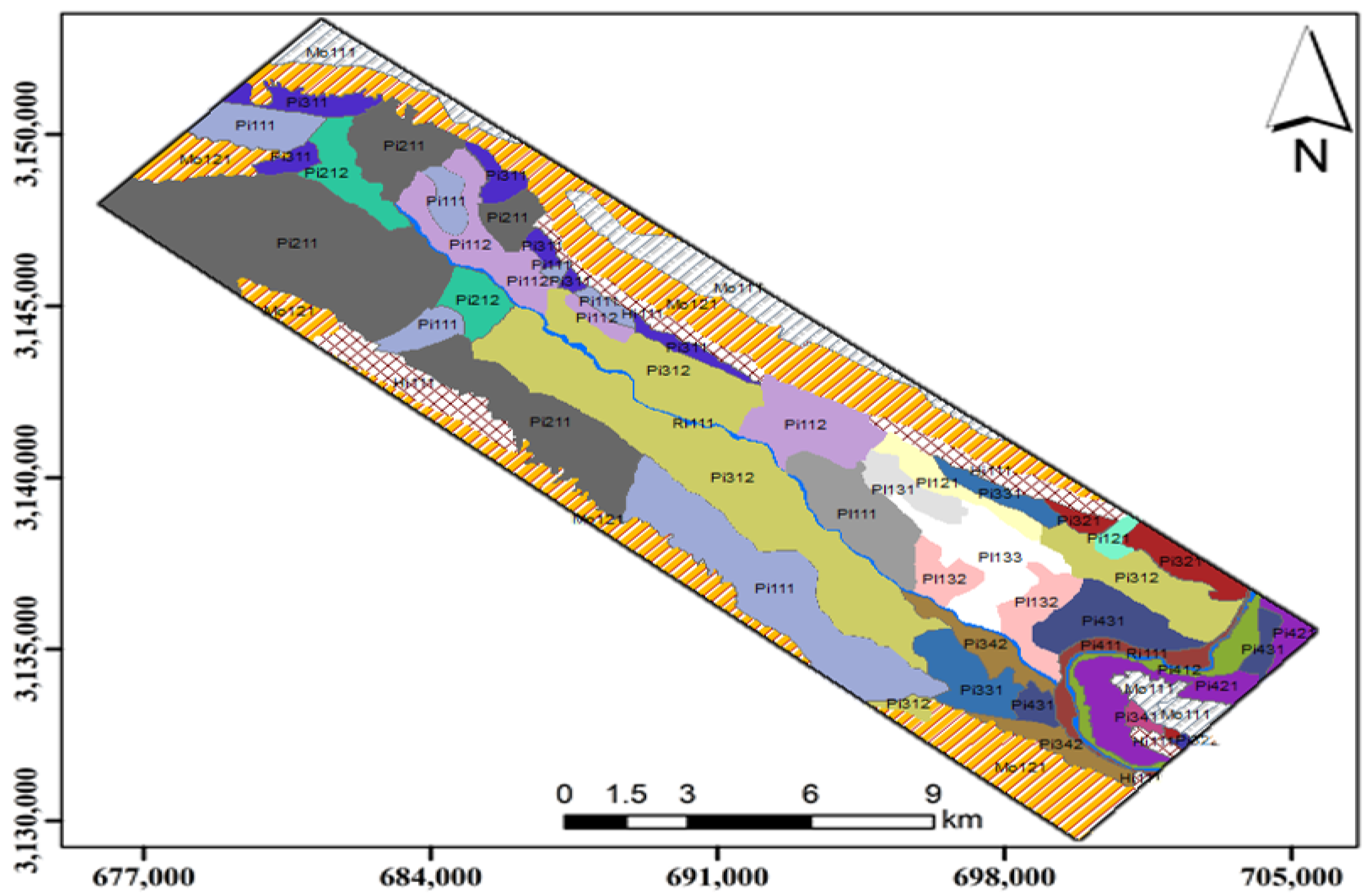
2.3.4. Geology and Geomorphology Maps

Other valuable sources of information for assessing soil properties are geology and geomorphology maps that present soil parent material and soil genesis, and other soil-forming factors, especially in arid regions [12,68]. The geomorphic units were determined using a nested hierarchy described by Toomanian et al. [61]. For the purpose of the breakdown of the intricacy of various landscapes, a four-level geomorphic hierarchy was used in this method: landscapes, landforms, lithology, and geomorphology, and ultimately, 25 geomorphic units were mapped (Figure 2 and Table 1).

2.4. Preprocessing and Feature Selection

When a model has a high number of predictors, improving its performance and general capabilities requires an exhaustive search of all possible subsets to choose the best predictors [70,71]. Furthermore, several of the models in the caret package do not need all the predictors, and using feature selection for these models would be more efficient [72].
Three scenarios were investigated to determine the capability of the combined RS and PS data, topographic attributes, geology map, and geomorphology map to estimate ECe, including:
Scenario (1): Using only 9 SySI bands and 13 salinity indices derived from SySI; Scenario (2): Using RS data (10 Sentinel multispectral bands, 13 salinity indices, and 6 vegetation indices), PS data (ECa and elemental concentration by pXRF), topographic attributes (21 attributes extracted from DEM), and geology and geomorphology maps; and Scenario (3): Using total variables including RS data (10 Sentinel multispectral bands, 13 salinity indices, and 6 vegetation indices), 9 SySI bands and 13 salinity indices derived from SySI, PS data (ECa and elemental concentration by pXRF), topographic attributes (21 attributes extracted from DEM), and geology and geomorphology maps to estimate ECe.

2.5. Modeling Approaches

For modeling, the following preprocessing was applied to the data. Because the ECe data had a log-normal distribution, it was log-transformed before being preprocessed and modeled. First, the variance inflation factor (VIF) was calculated for each covariate to check the impact of multicollinearity in each MLR model and covariates with VIF >10 were removed from the datasets [73]. In the next step, the Boruta method was applied to select the most important covariates with the target covariate (ECe). Then, a linear technique represented partial least squares regression (PLSR), and three non-linear techniques, artificial neural networks (ANN), random forest (RF), and support vector machines (SVM), were used for modeling. In addition, k-nearest neighbors (kNN) was considered a non-parametric algorithm necessary for accurately modeling non-linear data and interpolating point source soil data across the landscape [74]. Then, the final ensemble model was composed of five individual predictions (one for each calibration technique), which were weighted averaged [19]. All feature selections and modeling were performed using the “caret” and “caretEnsemble” packages in R 3.5.2 [66].
The Pearson correlation coefficients were calculated between soil salinity from the topsoil (0–30 cm) and environmental covariates. The statistical analysis was performed in the R environment [66], using the package corrplot [75].

2.6. Assessment of Model Performance

The prediction performance of models was assessed using 10-fold cross-validation [76]. Cross-validation provides a structure for creating several train/test splits in the dataset and guaranteeing that each data point is in the test set at least once. The advantage of this method is that it performs reliably and is unbiased on smaller datasets. To compare the modeling performance and determine the optimal model, the coefficient of determination (R2), root mean square error (RMSE), mean absolute error (MAE), and normalized root mean square error (nRMSE) were calculated. RMSE means show how close the predicted values are to the observed values, and the coefficient of determination (R2) shows the proportion of the variance in the target covariate that the model explains.
R 2 = 1 i = 1 n ( Z * ( X i ) Z ( X i ) ) 2 i = 1   n ( Z ( X i ) Z ¯ ( X ) ) 2
R M S E = [ i = 1 N [ Z ( X i ) Z * ( X i ) ] 2 N ] 1 / 2
M A E = 1 N i = 1 N [ | Z ( X i ) Z * ( X i ) | ]
n R M S E =   R M S E Z ¯ ( X ) × 100
where Z(Xi) and Z∗(Xi) are the observed and predicted values, respectively, and Z ¯ ( X ) is the average of observed values, and N is the number of measurements.

3. Results

3.1. Descriptive Statistics of Field Measurements (ECe, ECa, and pXRF)

Table 3 presents the descriptive statistics of ECe, EM38 readings, and concentrations of elements measured with pXRF. The ECe showed a broad range from 0.48 to 73.92 dS m−1, while the log-transformed ECe values ranged from −0.31 to 1.87 log10 dS m−1 (Table 3). These values were used as the dependent covariate for modeling (Table 4). The ECav ranged between 7 and 431 mS m−1 with a mean value of 45.92 mS m−1, whereas the ECah varied from 3 to 198 mS m−1 with an average of 26.64 mS m−1. The coefficients of variation (CV) for ECe, ECav, and ECah were 150.43, 128.25, and 117.90%, respectively (Table 3).
According to the soil salinity classification, the U.S. Salinity Laboratory Staff [52], 11% of the soil samples were strongly saline (≥16 dS m−1), 18% moderately (8–16 dS m−1), 13% slightly (4–8 dS m−1), 15% very slightly (2–4 dS m−1), and 43% non-saline (0–2 dS m−1).
The results showed that 42% of samples had an ECe of more than 4 dS m−1, indicating salt-affected soils. The pXRF instrument was used to measure K, Ca, S, and C elements and these were applied for soil salinity modeling. CV for K, Ca, S, and Cl contents were 18.84, 18.62, 368.34, and 105.42%, respectively (Table 3). Among the measured elements, the highest mean (285,170 mg Kg−1) was related to Ca. This is probably due to the accumulation of calcium carbonate in the soils of this region (Table 3). In the arid and semi-arid regions, calcium carbonates accumulate in the top-surface due to high temperatures and low precipitation amounts [77].

3.2. Correlations between ECe and Environmental Covariates

Since the present study aimed to investigate the effects of using auxiliary covariates independently and in combination on soil salinity as a target covariate, the VIF procedure was used to reduce variables. The covariate reduction has been used to reduce errors in predictions [78] through the removal of potentially irrelevant predictor covariates. Since weak learners produce weak outliers, the process progressively increases the prediction accuracy by reducing the chance of obtaining outliers [79]. A total of 51 covariates were derived from the RS data, and 7 covariates were retained. Of the six covariates from the PS data, five remained, while out of 21 topographic attributes extracted from DEM, only four covariates were included in the final environmental dataset. Finally, Pearson’s correlation analysis was performed, and a correlogram was constructed to investigate the sensitivity of the remaining environmental factors to soil salinity (Figure 4). Soil salinity showed a high correlation with the PS data, relatively weak correlation with topographic attributes, and low correlation with the RS data (Figure 4). Therefore, PS data could play an important role in prediction and improving the accuracy of ECe. PS data including Cl, ECav, and ECah showed a positive correlation, while K and Ca negatively correlated with soil salinity (Figure 4).
Among the four topographic attributes, the correlation between MRVBF and ECe was positive and high; however, CNBL, Val_Dep, RSP, and ECe showed a negative correlation with ECe. The highest correlation was related to CNBL, followed by MRVBF, Val_Dep, and RSP (Figure 4). The results showed a weak correlation between the covariates derived from RS, including spectral bands, vegetation indices, salinity indices, and ECe (Figure 4).

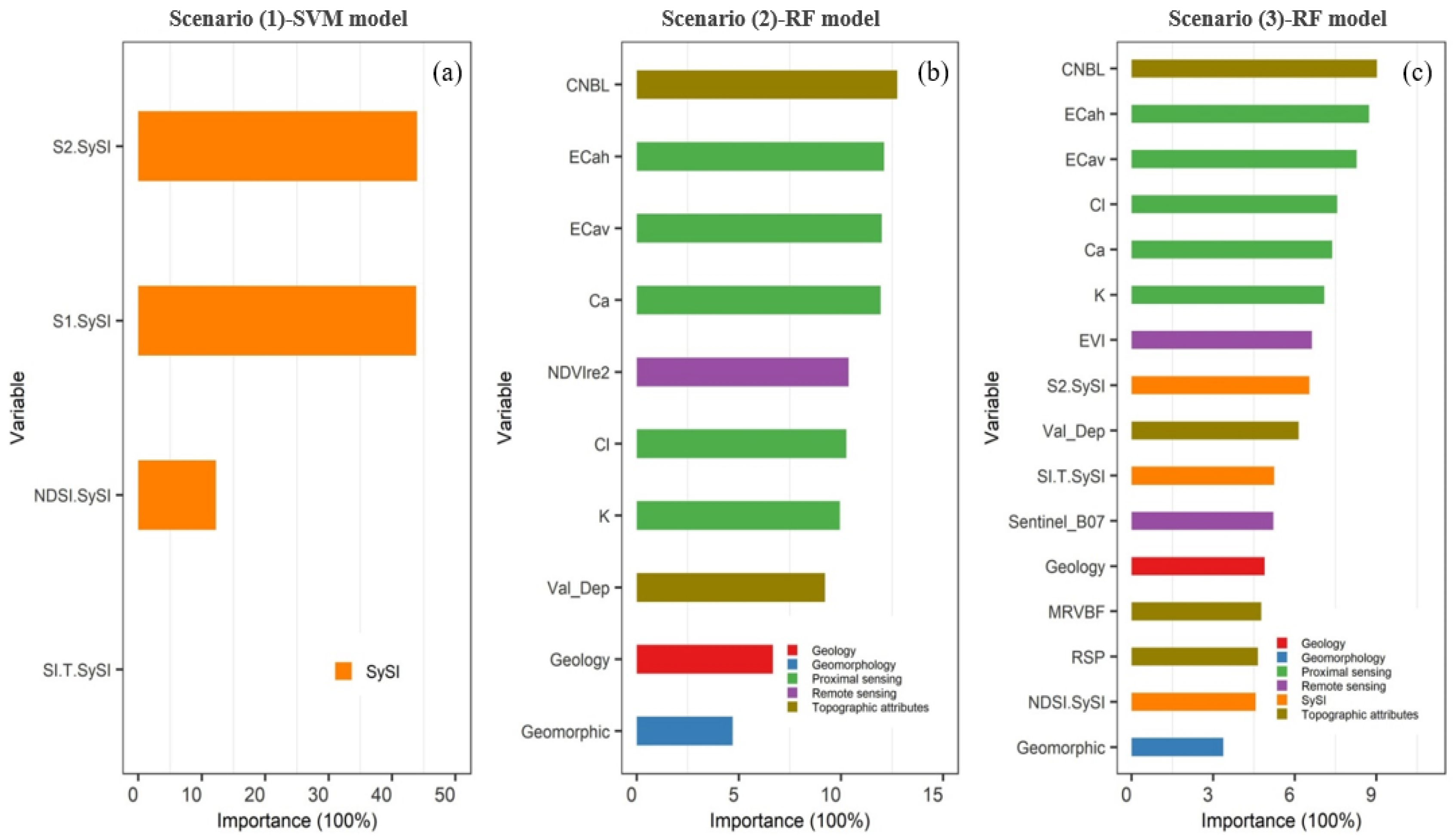
3.3. Covariate Importance

Figure 5 shows the measured importance of the examined predictor covariates taken from the Boruta algorithm for each scenario. The results showed that salinity indices were obtained from SySI, including S2.SySI, S1.SySI, and NDSI.SySI, and are the most important covariates for predicting ECe in Scenario (1) (Figure 5a). In Scenario (2), the PS data (ECah, ECav, Ca, Cl, and K) with 56% of total relative importance were the main covariates for predicting ECe content. Just afterward came the topographic attributes (CNBL and Val_Dep) with 22%, RS data (NDVIre2) with 12%, and geology and geomorphology maps with 10% as important covariates for predicting soil salinity (Figure 5b). In Scenario (3), the highest importance was related to the PS data (ECav, ECah, Ca, Cl, and K) with 40% of the total relative importance, followed by topographic attributes (CNBL, Val_Dep, MRVBF, and RSP) with 23%, salinity indices obtained from SySI (S2.SySI, S1.SySI, and NDSI.SySI) with 17%, RS data (EVI and Sentinel_B07) with 12%, and geology and geomorphology maps with 8% were the most important covariates for predicting ECe (Figure 5c).

3.4. Modeling Performance and Evaluation

The performance of models (i.e., kNN, ANN, PLS, RF, SVM, and ensemble model) for predicting ECe content in each scenario was compared based on R2, MAE, RMSE, and nRMSE indices (Table 4). The best prediction accuracy was obtained using the SVM model in Scenario (1), while the RF model outperformed in the others ((2) and (3)) (Table 4). However, the comparison between all scenarios showed that the best prediction accuracy is obtained for the RF model in Scenario (3) (R2 = 0.48 and RMSE = 2.49), followed by Scenario (2) for the RF model (R2 = 0.47 and RMSE = 2.50), and then Scenario (1) for the SVM model (R2 = 0.26 and RMSE = 2.97). Comparison of three scenarios showed that there was a difference between the models developed with Scenarios (1) and (2) and Scenarios (1) and (3). However, there was a little difference between the developed models with Scenarios (2) and (3). In ECe modeling, the difference in the value of R2 for the best model was 0.21 in Scenarios (1) and (2) and 0.22 in Scenarios (1) and (3), but the R2 value differed 0.01 for the best model in Scenarios (2) and (3) (Figure 5 and Table 4). We employed the ensemble modeling technique to see whether we could enhance the prediction of soil salinity (Table 4). Results showed that the ensemble model had the best performance in Scenario (3) with R2 = 0.79 and RMSE = 1.76, followed by Scenario (2) with R2 = 0.73 and RMSE = 1.89, and then Scenario (1) with R2 = 0.58 and RMSE = 2.22 (Table 4). This indicates that the ensemble modeling approach produced more accurate and dependable predictive soil salinity results than the individual models (Table 4). Relative improvement (RI%) indicated that the R2 index in the ensemble model improved compared with the most accurate prediction for Scenarios (1), (2), and (3) with 120.95, 56.82, and 66.71%, respectively (Table 4).
Results indicated that PS data and topographic attributes are important in predicting ECe, and better results were obtained when all auxiliary covariates (RS and PS data, salinity indices obtained from SySI, topographic attributes, and geology and geomorphology maps) for salinity prediction were combined (Table 4). Moreover, the results demonstrated that the selection of environmental covariates influences prediction accuracy (Table 4). Environmental covariates derived from SySI had a low correlation with ECe, which is possibly the reason for the low accuracy estimation in Scenario (1) (Figure 4 and Table 4).

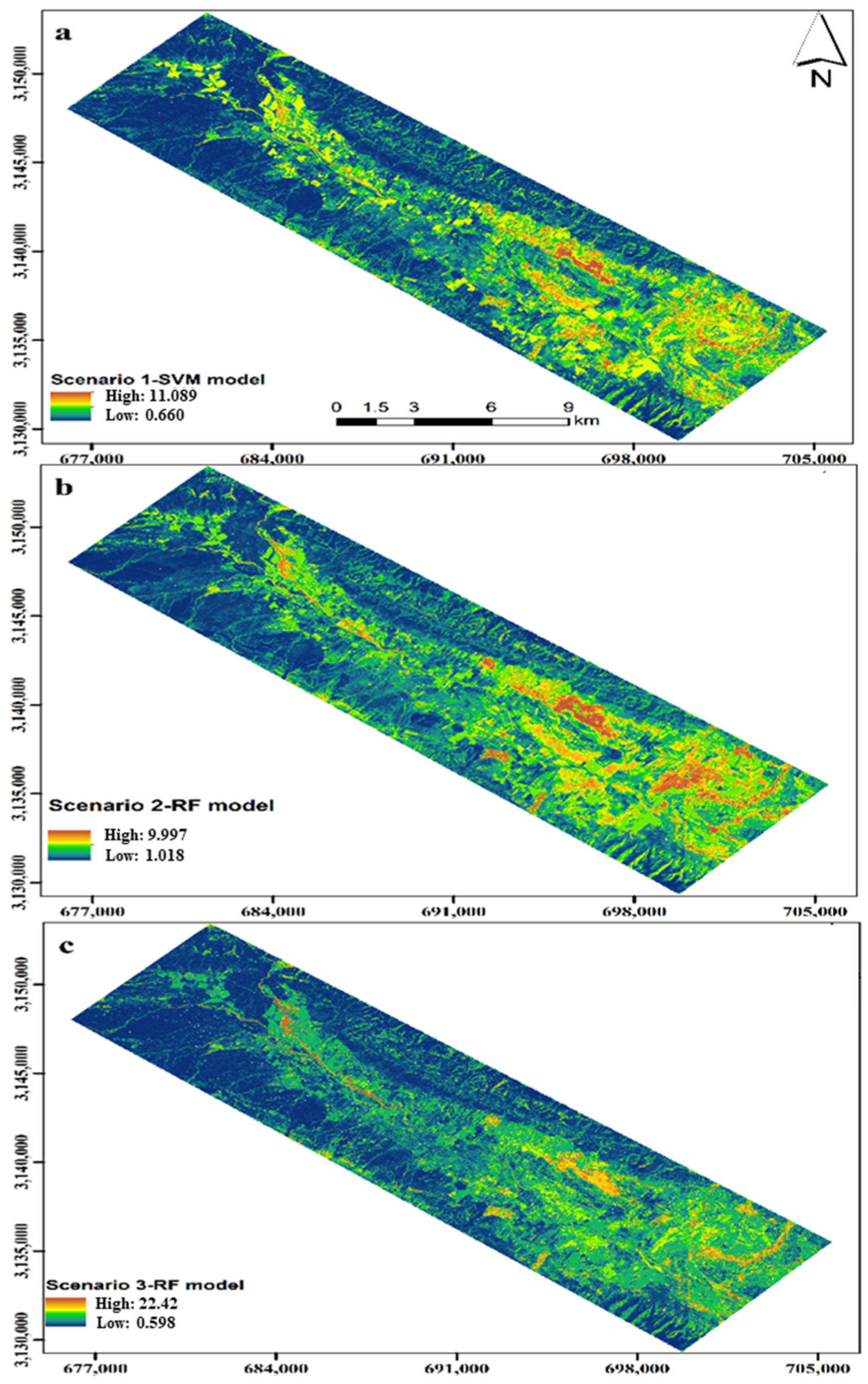
3.5. Spatial Distribution of Soil Salinity

Figure 6 shows the spatial distribution of ECe using the best performance model for three scenarios. The spatial patterns of ECe produced for the three scenarios corresponded with the distribution of known topographic features in the region. The prediction maps of ECe by the three scenarios indicated that ECe tended to increase from northwestern to south and southeastern regions. The regions with high ECe were located in low elevations and playa, where halophyte plant Suaeda aegyptiaca grows. The regions with low ECe were located in the higher elevations with steeper slopes and alluvial fans (Figure 1 and Figure 6). A large amount of salt is likely discharged from the middle and upper parts of the alluvial fans [12]. The discharged salts flow to the surrounding area at a low altitude in central and southern areas (Figure 1 and Figure 6). Generally, this is because the higher sections of the area have a sandy texture and low salt absorbability. There occurs leaching and discharge of salts to the lower parts, which have a clay texture and poor drainage (Figure 6). The spatial patterns of ECe also corresponded with the lithological map so that the soil of the southern parts generally has a geological formation Q s c s and Q s c 1 , which contains salt (Figure 1a and Figure 6). As shown in Figure 6, three scenarios predicted low ECe values appropriately; however, the high ECe values are relatively underestimated. The minimum predicted ECe by Scenario (1) is 0.660 dS m−1, and the maximum is 11.089 dS m−1 (Figure 6a), while the maximum ECe by Scenarios (2) and (3) are 9.997 dS m−1 and 22.42 dS m−1, respectively (Figure 6b,c).

4. Discussion

In the study, ground observations and environmental covariates were integrated to map soil salinity. This property has a wide range in the study area. This is likely due to the fact that landscape position, soil type, parent material, and other variables influence soil salinity variations [80]. Additionally, soil salinity changes quickly over short distances due to topography and other variables [81]. Therefore, we used RS and PS techniques to predict soil salinity as the cost and time-efficient approach. In this study, we obtained a lower CV for ECah and ECav values than ECe, which was consistent with the results of Taghizadeh-Mehrjardi et al. [4]. They stated this is because the instrument measures ECa in a larger soil volume, while smaller soil samples were measured for ECe.
In a study conducted in Texas, the USA, Aldabaa et al. [18] predicted soil salinity by combining RS data and content of soil elements measured by pXRF. They reported that S and Cl had the highest CV values among the elements, which indicated outliers for these two elements. Similarly, among the elements measured by pXRF, S and Cl had the highest CV in this study.
The positive correlation between soil salinity and Cl indicates that the origin of salinity in the region is probably salts that contain Cl (halite). Aldabaa et al. [18] also reported a high correlation between log10 EC with S (0.78) and Cl (0.60). The authors stated that the high correlation indicated the origin of salinity when salts contain SO4 (gypsum) and Cl (halite). They also reviewed the results of energy-dispersive X-ray spectroscopy and found that S, Na, Mg, O, Cl, K, Al, and Ca were prevalent elements in high salinity samples (especially Cl and S). On the other hand, they found that Ca, Mg, Si, K, O, and Al are prevalent elements in non-saline samples. This finding is consistent with the result of the negative correlation between ECe and Ca and K in our study.
Although the study area comprises several land uses, geological formations, and geomorphic surfaces (Figure 1 and Figure 4), it could be concluded that the relatively weak correlations between topographic attributes and soil salinity are probably because the study area has a relatively flat topographic system in most of the area [82]. In addition, due to the flatness in the middle and southern parts of the area, surface runoff due to precipitation was limited, preventing salts’ redistribution [68,83].
Peng et al. [68], working in southern Xinjiang Province, China, reported that CNBL and RSP variables, among the topographic attributes, have a significant negative correlation with salinity, and this result was consistent with our finding. According to previous research [84,85], some topography indices (elevation, RSP, Val_Dep, and CNBL) have a strong relationship with EC and significantly affect other soil characteristics. In a study in Dongying City, Shandong Province, China, Yang et al. [82] obtained a high correlation between elevation and total salt content. They attributed this to the effect of elevation on groundwater level, which significantly impacts water and salt migration. Moreover, they have reported a very weak correlation between profile curvature, plan curvature, and TWI with total salt due to the flatness of the region. In agreement with our findings, Akramkhanov et al. [83], in a study in Khorezm Province, Uzbekistan, reported that most terrain attributes had a low correlation with topsoil properties and bulk salinity, as their study area was rather flat.
Different spectral behaviors affected by variable rates of soil salinity are the basis for monitoring surface soil salinity using RS data [29]. In different works, spectral bands and a salinity index [86,87,88] have been directly used as a vegetation index [56,84,88] with an indirect approach. The low correlation between satellite data and soil salinity is probably due to the fact that a small part of the study area has a salinity of more than 8 dS m−1, and salinity is not visible at the soil surface) Figure 4). Moreover, in some parts of the area, the white color on the soil surface is due to the presence of gypsum or surface gravel, which causes errors in salinity monitoring using satellite data. Zeraatpisheh et al. [89] reported that when the study area has low vegetation indices (e.g., NDVI lower than 0.3), there is no or very low correlation between RS covariates and soil organic carbon content.
The corresponding reflectance characteristics of the eight representative soil samples with different ECe for the SySI and Sentinel-2A band showed that samples with ECe of 66.02 and 33.21 dS m−1 attained a higher reflectance than the other samples in the SySI band. In contrast, in the Sentinel-2A band, soil samples with an ECe 66.02 dS m−1 showed the highest reflectance (Figure 7a,b). The reflectance curve of the soil samples in the SySI band with an ECe ranging from 0.53 to 16.38 dS m−1 was more concentrated, and the reflectance in the nine wavebands was low (Figure 7). In this study, the soil samples with the lowest and highest ECe did not correspond to the lowest and highest reflectance curves, respectively, which should be closely related to the salt composition, soil moisture content [90,91], and other soil properties such as gypsum, carbonate, soil organic carbon, and soil texture. Wang et al. [5] stated that areas covered by a white salt crust have a large amount of salt. They also indicated that the spectral reflectance of the soil samples does not necessarily increase with increasing soil salinity in each band of the Sentinel-2 MSI data. This fact makes it difficult to map and monitor the soil surface salinity using multispectral bands and their derived indices. It can also be observed that spectral behavior has a trend where the spectra increase from lower to higher ECe (from visible to SWIR2), forming an angle. In both cases, the trend of SySI and Sentinel maintained the higher ECe with greater reflectance and increased type.
The results indicated that the RF and SVM models had a higher performance in predicting soil salinity among the models investigated (Table 4). These higher accuracies are due to the ability of the algorithms to handle the non-linear relationships, which are typically observed between soil salinity, ground observations, and environmental covariates. Although the differences between the modeling performance in Scenarios (2) and (3) are not significant, the most important factors affecting model performance are mainly sample density and input variables. Since the number of samples in this study was consistent in two scenarios, different environmental variables in the two scenarios induced different performances [13]. In a study in Aksu Province, China, Wang et al. [5] indicated that the SVM soil EC estimation model had higher performance and accuracy than soil EC estimation models created with ANN and RF models. In a study conducted in southern Xinjiang, China, Wang et al. [79] found that RF was the best algorithm for predicting soil salinity in arid regions.
The modeling results showed that the ensemble soil ECe estimation model performed better than the individual approaches (Table 4). This is because the polynomial ensemble model can combine the strengths of individual ones [26]. The ensemble model improved the validation indicators positively compared to the best individual model in all scenarios (Table 4). According to Heung et al. [92], ensemble learning is a strategy for improving the consistency of results in soil surveys with complicated relationships between variables.
In many previous studies, regions with vegetation coverage were directly identified as non- or slightly salinized [93,94]. However, in our study, areas with high salinity also have vegetation because these areas are generally irrigated with saltwater, and salt-tolerant plants such as barley, wheat, and dates are grown. Because of differences in topography, vegetation kinds, and geographic location, the soil salinity under vegetation cover varied from non-saline to heavily saline soil [95,96].
Our results showed that the covariates obtained from PS are more important and practical predictors of soil salinity than RS. These results were consistent with previous studies [18,36]. The data also showed that ECah and ECav were more important among the PS data (Figure 5), which is confirmed by the results of Taghizadeh-Mehrjardi et al. [4]. These authors reported that ECav was the most important covariate for predicting ECe in surface soils.

5. Conclusions

The present study was conducted to investigate the spatial variation of soil salinity using multiple machine learnings and environmental covariates in an arid region in Iran. Since EMI is sensitive to soil salinity and moisture, and pXRF directly measures constituent soil elements that play a role in soil salinity (Cl), PS showed a higher correlation than RS and topographic attributes. The low correlation between satellite data and soil salinity is probably because salt is not visible at the soil surface. Thus, our results showed that covariates obtained from PS are more important than RS covariates and could be more precise to predict soil salinity. The results showed that the ensemble model was generally successful, as it produced a more accurate prediction for soil salinity than individual ones. The ensemble modeling method positively improved the validation indicators more than the best individual model in all scenarios.
We propose that the PS, RS data, and topographic attributes be merged for optimal soil salinity prediction because these data types are inexpensive, easy, and rapid to obtain and can be used for soil salinity management. The results of this study showed that the combination of PS and RS data with topographic attributes could be successfully used to monitor and map other basic soil properties such as textural constituents, soil pH, carbonate, gypsum, and soil organic carbon in the future. In doing so, researchers will be able to achieve results that are comparable to lab-derived data while spending less time and making less attempts than traditional laboratory determinations.

Author Contributions

Conceptualization, S.N. and M.Z.; Methodology, S.N. and M.Z.; Software, S.N. and M.Z.; Validation, S.N. and M.Z.; Resources, S.A. and J.A.M.D.; Writing—original draft preparation, S.N. and M.Z.; Writing—review and editing, S.N., S.A., M.Z. and J.A.M.D.; Visualization, S.N. and M.Z. All authors have read and agreed to the published version of the manuscript.

Funding

This research was supported by grants from the Iran National Science Foundation (INSF) (Grant Nos. 98001941).

Institutional Review Board Statement

Not applicable.

Informed Consent Statement

Not applicable.

Data Availability Statement

The data presented in this study are available on request form the corresponding author.

Acknowledgments

The authors would like to thank the Geotechnology in Soil Science Group, GEOCIS (http://esalqgeocis.wix.com/english, accessed on 23 November 2021) at the Soil Science Department at the University of São Paulo for providing excellent support services, and FAPESP n. 2014-2262-0. The authors also acknowledge the Iran National Science Foundation (INSF) financial support for project No: 98001941, which made the study possible. Mojtaba Zeraatpisheh’s postdoctoral program at Henan University, China, has been supported by the National Key Research and Development Program of China, grant numbers 2017YFA0604302 and 2018YFA0606500.

Conflicts of Interest

The authors declare no conflict of interest.

References

  1. El Harti, A.; Lhissou, R.; Chokmani, K.; Ouzemou, J.; Hassouna, M.; Bachaoui, E.M.; El Ghmari, A. Spatiotemporal Monitoring of Soil Salinization in Irrigated Tadla Plain (Morocco) Using Satellite Spectral Indices. Int. J. Appl. Earth Obs. Geoinf. 2016, 50, 64–73. [Google Scholar] [CrossRef]
  2. Zaman, M.; Shahid, S.A.; Heng, L. Irrigation Systems and Zones of Salinity Development. In Guideline for Salinity Assessment, Mitigation and Adaptation Using Nuclear and Related Techniques; Springer International Publishing: Cham, Switzerland, 2018; pp. 91–111. ISBN 978-3-319-96189-7. [Google Scholar]
  3. Farahmand, N.; Sadeghi, V. Estimating Soil Salinity in the Dried Lake Bed of Urmia Lake Using Optical Sentinel-2 Images and Nonlinear Regression Models. J. Indian Soc. Remote Sens. 2020, 48, 675–687. [Google Scholar] [CrossRef]
  4. Taghizadeh-Mehrjardi, R.; Minasny, B.; Sarmadian, F.; Malone, B.P. Digital Mapping of Soil Salinity in Ardakan Region, Central Iran. Geoderma 2014, 213, 15–28. [Google Scholar] [CrossRef]
  5. Wang, J.; Peng, J.; Li, H.; Yin, C.; Liu, W.; Wang, T.; Zhang, H. Soil Salinity Mapping Using Machine Learning Algorithms with the Sentinel-2 MSI in Arid Areas, China. Remote Sens. 2021, 13, 305. [Google Scholar] [CrossRef]
  6. Li, J.; Pu, L.; Zhu, M.; Dai, X.; Xu, Y.; Chen, X.; Zhang, L.; Zhang, R. Monitoring Soil Salt Content Using HJ-1A Hyperspectral Data: A Case Study of Coastal Areas in Rudong County, Eastern China. Chin. Geogr. Sci. 2015, 25, 213–223. [Google Scholar] [CrossRef]
  7. McBratney, A.B.; Mendonça Santos, M.L.; Minasny, B. On Digital Soil Mapping. Geoderma 2003, 117, 3–52. [Google Scholar] [CrossRef]
  8. McBratney, A.; Field, D.; Morgan, C.L.S.; Huang, J. On Soil Capability, Capacity, and Condition. Sustainability 2019, 11, 3350. [Google Scholar] [CrossRef] [Green Version]
  9. Viscarra Rossel, R.A.; Behrens, T.; Ben-Dor, E.; Brown, D.J.; Demattê, J.A.M.; Shepherd, K.D.; Shi, Z.; Stenberg, B.; Stevens, A.; Adamchuk, V.; et al. A Global Spectral Library to Characterize the World’s Soil. Earth-Sci. Rev. 2016, 155, 198–230. [Google Scholar] [CrossRef] [Green Version]
  10. Hengl, T.; Mendes de Jesus, J.; Heuvelink, G.B.M.; Ruiperez Gonzalez, M.; Kilibarda, M.; Blagotić, A.; Wei, S.; Wright, M.N.; Geng, X.; Bauer-Marschallinger, B.; et al. SoilGrids250m: Global Gridded Soil Information Based on Machine Learning. PLoS ONE 2017, 12, e0169748. [Google Scholar] [CrossRef] [Green Version]
  11. Goydaragh, M.G.; Taghizadeh-Mehrjardi, R.; Jafarzadeh, A.A.; Triantafilis, J.; Lado, M. Using Environmental Variables and Fourier Transform Infrared Spectroscopy to Predict Soil Organic Carbon. CATENA 2021, 202, 105280. [Google Scholar] [CrossRef]
  12. Jafari, A.; Finke, P.A.; Vande Wauw, J.; Ayoubi, S.; Khademi, H. Spatial Prediction of USDA- Great Soil Groups in the Arid Zarand Region, Iran: Comparing Logistic Regression Approaches to Predict Diagnostic Horizons and Soil Types. Eur. J. Soil Sci. 2012, 63, 284–298. [Google Scholar] [CrossRef]
  13. Zeraatpisheh, M.; Jafari, A.; Bagheri Bodaghabadi, M.; Ayoubi, S.; Taghizadeh-Mehrjardi, R.; Toomanian, N.; Kerry, R.; Xu, M. Conventional and Digital Soil Mapping in Iran: Past, Present, and Future. CATENA 2020, 188, 104424. [Google Scholar] [CrossRef]
  14. Ma, Y.; Minasny, B.; Welivitiya, W.D.D.P.; Malone, B.P.; Willgoose, G.R.; McBratney, A.B. The Feasibility of Predicting the Spatial Pattern of Soil Particle-Size Distribution Using a Pedogenesis Model. Geoderma 2019, 341, 195–205. [Google Scholar] [CrossRef]
  15. Naimi, S.; Ayoubi, S.; Demattê, J.A.M.; Zeraatpisheh, M.; Amorim, M.T.A.; de Oliveira Mello, F.A. Spatial Prediction of Soil Surface Properties in an Arid Region Using Synthetic Soil Image and Machine Learning. Geocarto Int. 2021. [Google Scholar] [CrossRef]
  16. Hosseini, M.; Rajabi Agereh, S.; Khaledian, Y.; Jafarzadeh Zoghalchali, H.; Brevik, E.C.; Movahedi Naeini, S.A.R. Comparison of Multiple Statistical Techniques to Predict Soil Phosphorus. Appl. Soil Ecol. 2017, 114, 123–131. [Google Scholar] [CrossRef]
  17. Emadi, M.; Taghizadeh-Mehrjardi, R.; Cherati, A.; Danesh, M.; Mosavi, A.; Scholten, T. Predicting and Mapping of Soil Organic Carbon Using Machine Learning Algorithms in Northern Iran. Remote Sens. 2020, 12, 2234. [Google Scholar] [CrossRef]
  18. Aldabaa, A.A.A.; Weindorf, D.C.; Chakraborty, S.; Sharma, A.; Li, B. Combination of Proximal and Remote Sensing Methods for Rapid Soil Salinity Quantification. Geoderma 2015, 239–240, 34–46. [Google Scholar] [CrossRef] [Green Version]
  19. Tajik, S.; Ayoubi, S.; Zeraatpisheh, M. Digital Mapping of Soil Organic Carbon Using Ensemble Learning Model in Mollisols of Hyrcanian Forests, Northern Iran. Geoderma Reg. 2020, 20, e00256. [Google Scholar] [CrossRef]
  20. Mondal, A.; Khare, D.; Kundu, S.; Mondal, S.; Mukherjee, S.; Mukhopadhyay, A. Spatial Soil Organic Carbon (SOC) Prediction by Regression Kriging Using Remote Sensing Data. Egypt. J. Remote Sens. Space Sci. 2017, 20, 61–70. [Google Scholar] [CrossRef] [Green Version]
  21. Shen, Q.; Wang, Y.; Wang, X.; Liu, X.; Zhang, X.; Zhang, S. Comparing Interpolation Methods to Predict Soil Total Phosphorus in the Mollisol Area of Northeast China. CATENA 2019, 174, 59–72. [Google Scholar] [CrossRef]
  22. Forkuor, G.; Hounkpatin, O.K.L.; Welp, G.; Thiel, M. High Resolution Mapping of Soil Properties Using Remote Sensing Variables in South-Western Burkina Faso: A Comparison of Machine Learning and Multiple Linear Regression Models. PLoS ONE 2017, 12, e0170478. [Google Scholar] [CrossRef]
  23. Amirian-Chakan, A.; Minasny, B.; Taghizadeh-Mehrjardi, R.; Akbarifazli, R.; Darvishpasand, Z.; Khordehbin, S. Some Practical Aspects of Predicting Texture Data in Digital Soil Mapping. Soil Tillage Res. 2019, 194, 104289. [Google Scholar] [CrossRef]
  24. Poppiel, R.R.; Demattê, J.A.M.; Rosin, N.A.; Campos, L.R.; Tayebi, M.; Bonfatti, B.R.; Ayoubi, S.; Tajik, S.; Afshar, F.A.; Jafari, A.; et al. High Resolution Middle Eastern Soil Attributes Mapping via Open Data and Cloud Computing. Geoderma 2021, 385, 114890. [Google Scholar] [CrossRef]
  25. Mohammed, S.; Al-Ebraheem, A.; Holb, I.J.; Alsafadi, K.; Dikkeh, M.; Pham, Q.B.; Linh, N.T.T.; Szabo, S. Soil Management Effects on Soil Water Erosion and Runoff in Central Syria—A Comparative Evaluation of General Linear Model and Random Forest Regression. Water 2020, 12, 2529. [Google Scholar] [CrossRef]
  26. Taghizadeh-Mehrjardi, R.; Minasny, B.; Toomanian, N.; Zeraatpisheh, M.; Amirian-Chakan, A.; Triantafilis, J. Digital Mapping of Soil Classes Using Ensemble of Models in Isfahan Region, Iran. Soil Syst. 2019, 3, 37. [Google Scholar] [CrossRef] [Green Version]
  27. Bannari, A.; El-Battay, A.; Bannari, R.; Rhinane, H. Sentinel-MSI VNIR and SWIR Bands Sensitivity Analysis for Soil Salinity Discrimination in an Arid Landscape. Remote Sens. 2018, 10, 855. [Google Scholar] [CrossRef] [Green Version]
  28. Taghadosi, M.M.; Hasanlou, M.; Eftekhari, K. Retrieval of Soil Salinity from Sentinel-2 Multispectral Imagery. Eur. J. Remote Sens. 2019, 52, 138–154. [Google Scholar] [CrossRef] [Green Version]
  29. Wang, J.; Ding, J.; Yu, D.; Teng, D.; He, B.; Chen, X.; Ge, X.; Zhang, Z.; Wang, Y.; Yang, X.; et al. Machine Learning-Based Detection of Soil Salinity in an Arid Desert Region, Northwest China: A Comparison between Landsat-8 OLI and Sentinel-2 MSI. Sci. Total Environ. 2020, 707, 136092. [Google Scholar] [CrossRef]
  30. Wang, J.; Ding, J.; Li, G.; Liang, J.; Yu, D.; Aishan, T.; Zhang, F.; Yang, J.; Abulimiti, A.; Liu, J. Dynamic Detection of Water Surface Area of Ebinur Lake Using Multi-Source Satellite Data (Landsat and Sentinel-1A) and Its Responses to Changing Environment. CATENA 2019, 177, 189–201. [Google Scholar] [CrossRef]
  31. Gorji, T.; Yildirim, A.; Hamzehpour, N.; Tanik, A.; Sertel, E. Soil Salinity Analysis of Urmia Lake Basin Using Landsat-8 OLI and Sentinel-2A Based Spectral Indices and Electrical Conductivity Measurements. Ecol. Indic. 2020, 112, 106173. [Google Scholar] [CrossRef]
  32. Viscarra Rossel, R.A.; Adamchuk, V.I.; Sudduth, K.A.; McKenzie, N.J.; Lobsey, C. Proximal Soil Sensing: An Effective Approach for Soil Measurements in Space and Time. In Advances in Agronomy; Elsevier: Amsterdam, The Netherlands, 2011; Volume 113, pp. 243–291. ISBN 978-0-12-386473-4. [Google Scholar]
  33. Grunwald, S.; Vasques, G.M.; Rivero, R.G. Fusion of Soil and Remote Sensing Data to Model Soil Properties. In Advances in Agronomy; Elsevier: Amsterdam, The Netherlands, 2015; Volume 131, pp. 1–109. ISBN 978-0-12-802136-1. [Google Scholar]
  34. Guo, Y.; Huang, J.; Shi, Z.; Li, H. Mapping Spatial Variability of Soil Salinity in a Coastal Paddy Field Based on Electromagnetic Sensors. PLoS ONE 2015, 10, e0127996. [Google Scholar] [CrossRef]
  35. Yao, R.; Yang, J.; Wu, D.; Xie, W.; Gao, P.; Jin, W. Digital Mapping of Soil Salinity and Crop Yield across a Coastal Agricultural Landscape Using Repeated Electromagnetic Induction (EMI) Surveys. PLoS ONE 2016, 11, e0153377. [Google Scholar] [CrossRef]
  36. Nouri, H.; Chavoshi Borujeni, S.; Alaghmand, S.; Anderson, S.; Sutton, P.; Parvazian, S.; Beecham, S. Soil Salinity Mapping of Urban Greenery Using Remote Sensing and Proximal Sensing Techniques; The Case of Veale Gardens within the Adelaide Parklands. Sustainability 2018, 10, 2826. [Google Scholar] [CrossRef] [Green Version]
  37. Ding, J.; Yang, S.; Shi, Q.; Wei, Y.; Wang, F. Using Apparent Electrical Conductivity as Indicator for Investigating Potential Spatial Variation of Soil Salinity across Seven Oases along Tarim River in Southern Xinjiang, China. Remote Sens. 2020, 12, 2601. [Google Scholar] [CrossRef]
  38. Swanhart, S.; Weindorf, D.C.; Chakraborty, S.; Bakr, N.; Zhu, Y.; Nelson, C.; Shook, K.; Acree, A. Soil Salinity Measurement Via Portable X-Ray Fluorescence Spectrometry. Soil Sci. 2014, 179, 417–423. [Google Scholar] [CrossRef]
  39. Vasques, G.M.; Rodrigues, H.M.; Coelho, M.R.; Baca, J.F.M.; Dart, R.O.; Oliveira, R.P.; Teixeira, W.G.; Ceddia, M.B. Field Proximal Soil Sensor Fusion for Improving High-Resolution Soil Property Maps. Soil Syst. 2020, 4, 52. [Google Scholar] [CrossRef]
  40. Silva, S.H.G.; dos Santos Teixeira, A.F.; de Menezes, M.D.; Guilherme, L.R.G.; de Souza Moreira, F.M.; Curi, N. Multiple Linear Regression and Random Forest to Predict and Map Soil Properties Using Data from Portable X-Ray Fluorescence Spectrometer (PXRF). Ciênc. Agrotec. 2017, 41, 648–664. [Google Scholar] [CrossRef]
  41. Silva, S.H.G.; Weindorf, D.C.; Faria, W.M.; Pinto, L.C.; Menezes, M.D.; Guilherme, L.R.G.; Curi, N. Proximal Sensor-Enhanced Soil Mapping in Complex Soil-Landscape Areas of Brazil. Pedosphere 2021, 31, 615–626. [Google Scholar] [CrossRef]
  42. Bilgili, A.V.; Cullu, M.A.; van Es, H.; Aydemir, A.; Aydemir, S. The Use of Hyperspectral Visible and Near Infrared Reflectance Spectroscopy for the Characterization of Salt-Affected Soils in the Harran Plain, Turkey. Arid Land Res. Manag. 2011, 25, 19–37. [Google Scholar] [CrossRef]
  43. Islamic Republic of Iran Meteorological Organization|GFCS. Available online: https://gfcs.wmo.int/node/65 (accessed on 23 November 2021).
  44. Fars Meteorological Bureau. Available online: https://www.farsmet.ir/ (accessed on 23 November 2021).
  45. Geological Map of Iran 1:100,000 Series [Cartographic Material]. Available online: https://nla.gov.au/nla.obj-233247255 (accessed on 23 November 2021).
  46. Soil Survey Staff Keys to Soil Taxonomy, 12th ed.; USDA-Natural Resources Conservation Service: Washington, DC, USA, 2014.
  47. Minasny, B.; McBratney, A.B. A Conditioned Latin Hypercube Method for Sampling in the Presence of Ancillary Information. Comput. Geosci. 2006, 32, 1378–1388. [Google Scholar] [CrossRef]
  48. Richards, L. Determination of the Properties of Saline and Alkali Soils. In Diagnosis and Improvement of Saline and Alkali Soils, Agriculture Handbook; No. 60; US Regional Salinity Laboratory: Riverside, CA, USA, 1954; Volume 60, pp. 7–33. [Google Scholar]
  49. Sparks, D.L. Methods of Soil Analysis. Part. 3: Chemical Methods; Soil Science Society of America, American Society of Agronomy: Madison, WI, USA, 1996; ISBN 978-0-89118-825-4. [Google Scholar]
  50. Sun, Y.; Cheng, Q.; Lin, J.; Schellberg, J.; Schulze Lammers, P. Investigating Soil Physical Properties and Yield Response in a Grassland Field Using a Dual-Sensor Penetrometer and EM38. Z. Pflanzenernähr. Bodenk. 2013, 176, 209–216. [Google Scholar] [CrossRef]
  51. Brevik, E.C.; Fenton, T.E.; Horton, R. Effect of Daily Soil Temperature Fluctuations on Soil Electrical Conductivity as Measured with the GeonicsÒ EM-38. Precis. Agric. 2004, 5, 145–152. [Google Scholar] [CrossRef]
  52. U.S. Salinity Laboratory Staff. Diagnosis and Improvement of Saline and Alcaly Soils; Handbook 60; USDA: Washington, DC, USA, 1954.
  53. Demattê, J.A.M.; Safanelli, J.L.; Poppiel, R.R.; Rizzo, R.; Silvero, N.E.Q.; de Sousa Mendes, W.; Bonfatti, B.R.; Dotto, A.C.; Salazar, D.F.U.; de Oliveira Mello, F.A.; et al. Bare Earth’s Surface Spectra as a Proxy for Soil Resource Monitoring. Sci. Rep. 2020, 10, 4461. [Google Scholar] [CrossRef] [PubMed]
  54. Douaoui, A.E.K.; Nicolas, H.; Walter, C. Detecting Salinity Hazards within a Semiarid Context by Means of Combining Soil and Remote-Sensing Data. Geoderma 2006, 134, 217–230. [Google Scholar] [CrossRef]
  55. Rahmati, M.; Mohammadi-Oskooei, M.; Neyshabouri, M.; Fakheri-Fard, A.; Ahmadi, A.; Walker, J. ETM+ Data Applicability for Remote Sensing of Soil Salinity in Lighvan Watershed, Northwest of Iran. Curr. Opin. Agric. 2014, 3, 10–13. [Google Scholar]
  56. Allbed, A.; Kumar, L. Soil Salinity Mapping and Monitoring in Arid and Semi-Arid Regions Using Remote Sensing Technology: A Review. ARS 2013, 02, 373–385. [Google Scholar] [CrossRef] [Green Version]
  57. Allbed, A.; Kumar, L.; Aldakheel, Y.Y. Assessing Soil Salinity Using Soil Salinity and Vegetation Indices Derived from IKONOS High-Spatial Resolution Imageries: Applications in a Date Palm Dominated Region. Geoderma 2014, 230–231, 1–8. [Google Scholar] [CrossRef]
  58. Cho, K.H.; Beon, M.-S.; Jeong, J.-C. Dynamics of Soil Salinity and Vegetation in a Reclaimed Area in Saemangeum, Republic of Korea. Geoderma 2018, 321, 42–51. [Google Scholar] [CrossRef]
  59. Qiu, Y.; Chen, C.; Han, J.; Wang, X.; Wei, S.; Zhang, Z. Satellite Remote Sensing Estimation Model of Soil Salinity in Jiefangzha Irrigation under Vegetation Coverage. Water Sav. Irrig. 2019, 44, 108–112. (In Chinese) [Google Scholar]
  60. Fan, X.; Pedroli, B.; Liu, G.; Liu, Q.; Liu, H.; Shu, L. Soil Salinity Development in the Yellow River Delta in Relation to Groundwater Dynamics. Land Degrad. Dev. 2012, 23, 175–189. [Google Scholar] [CrossRef]
  61. Toomanian, N.; Jalalian, A.; Khademi, H.; Eghbal, M.K.; Papritz, A. Pedodiversity and Pedogenesis in Zayandeh-Rud Valley, Central Iran. Geomorphology 2006, 81, 376–393. [Google Scholar] [CrossRef]
  62. Copernicus Open Access Hub. Available online: https://scihub.copernicus.eu/ (accessed on 23 November 2021).
  63. European Space Agency. Available online: https://www.esa.int/ (accessed on 23 November 2021).
  64. Demattê, J.A.M.; Fongaro, C.T.; Rizzo, R.; Safanelli, J.L. Geospatial Soil Sensing System (GEOS3): A Powerful Data Mining Procedure to Retrieve Soil Spectral Reflectance from Satellite Images. Remote Sens. Environ. 2018, 212, 161–175. [Google Scholar] [CrossRef]
  65. Main-Knorn, M.; Pflug, B.; Louis, J.; Debaecker, V.; Müller-Wilm, U.; Gascon, F. Sen2Cor for Sentinel-2. In Proceedings of the Image and Signal Processing for Remote Sensing XXIII, Warsaw, Poland, 4 October 2017; Bruzzone, L., Bovolo, F., Benediktsson, J.A., Eds.; SPIE: Warsaw, Poland, 2017; p. 3. [Google Scholar]
  66. R Core Team. R: A Language and Environment for Statistical Computing; R Foundation for Statistical Computing: Vienna, Austria, 2019. [Google Scholar]
  67. Gorji, T.; Sertel, E.; Tanik, A. Monitoring Soil Salinity via Remote Sensing Technology under Data Scarce Conditions: A Case Study from Turkey. Ecol. Indic. 2017, 74, 384–391. [Google Scholar] [CrossRef]
  68. Peng, J.; Biswas, A.; Jiang, Q.; Zhao, R.; Hu, J.; Hu, B.; Shi, Z. Estimating Soil Salinity from Remote Sensing and Terrain Data in Southern Xinjiang Province, China. Geoderma 2019, 337, 1309–1319. [Google Scholar] [CrossRef]
  69. Ministry of Economy, Trade and Industry of Japan, National Aeronautics and Space Administration. Available online: http://www.gdem.aster.ersdac.or.jp (accessed on 3 March 2021).
  70. Scull, P.; Franklin, J.; Chadwick, O.A. The Application of Classification Tree Analysis to Soil Type Prediction in a Desert Landscape. Ecol. Model. 2005, 181, 1–15. [Google Scholar] [CrossRef]
  71. Ließ, M.; Schmidt, J.; Glaser, B. Improving the Spatial Prediction of Soil Organic Carbon Stocks in a Complex Tropical Mountain Landscape by Methodological Specifications in Machine Learning Approaches. PLoS ONE 2016, 11, e0153673. [Google Scholar] [CrossRef] [Green Version]
  72. Kuhn, M. Variable Selection Using the Caret Package. Available online: http//cran.cermin.lipi.go.id/web/packages/caret/vignettes/caretSelection.pdf (accessed on 3 April 2021).
  73. Guo, L.; Fu, P.; Shi, T.; Chen, Y.; Zhang, H.; Meng, R.; Wang, S. Mapping Field-Scale Soil Organic Carbon with Unmanned Aircraft System-Acquired Time Series Multispectral Images. Soil Tillage Res. 2020, 196, 104477. [Google Scholar] [CrossRef]
  74. Mansuy, N.; Thiffault, E.; Paré, D.; Bernier, P.; Guindon, L.; Villemaire, P.; Poirier, V.; Beaudoin, A. Digital Mapping of Soil Properties in Canadian Managed Forests at 250m of Resolution Using the K-Nearest Neighbor Method. Geoderma 2014, 235–236, 59–73. [Google Scholar] [CrossRef]
  75. Wei, T.; Simko, V.; Levy, M.; Xie, Y.; Jin, Y.; Zemla, J.; Freidank, M.; Cai, J.; Protivinsky, T. Corrplot: Visualization of a Correlation Matrix. 2021. Available online: https://CRAN.R-project.org/package=corrplot/ (accessed on 23 November 2021).
  76. Hengl, T.; Heuvelink, G.B.M.; Kempen, B.; Leenaars, J.G.B.; Walsh, M.G.; Shepherd, K.D.; Sila, A.; MacMillan, R.A.; Mendes de Jesus, J.; Tamene, L.; et al. Mapping Soil Properties of Africa at 250 m Resolution: Random Forests Significantly Improve Current Predictions. PLoS ONE 2015, 10, e0125814. [Google Scholar] [CrossRef]
  77. Esfandiarpoor Borujeni, I.; Mohammadi, J.; Salehi, M.H.; Toomanian, N.; Poch, R.M. Assessing Geopedological Soil Mapping Approach by Statistical and Geostatistical Methods: A Case Study in the Borujen Region, Central Iran. CATENA 2010, 82, 1–14. [Google Scholar] [CrossRef]
  78. Svetnik, V.; Liaw, A.; Tong, C.; Culberson, J.C.; Sheridan, R.P.; Feuston, B.P. Random Forest: A Classification and Regression Tool for Compound Classification and QSAR Modeling. J. Chem. Inf. Comput. Sci. 2003, 43, 1947–1958. [Google Scholar] [CrossRef] [PubMed]
  79. Wang, F.; Shi, Z.; Biswas, A.; Yang, S.; Ding, J. Multi-Algorithm Comparison for Predicting Soil Salinity. Geoderma 2020, 365, 114211. [Google Scholar] [CrossRef]
  80. Clay, D.E.; Chang, J.; Malo, D.D.; Carlson, C.G.; Reese, C.; Clay, S.A.; Ellsbury, M.; Berg, B. Factors Influencing Spatial Variability of Soil Apparent Electrical Conductivity. Commun. Soil Sci. Plant. Anal. 2001, 32, 2993–3008. [Google Scholar] [CrossRef] [Green Version]
  81. Pozdnyakova, L.; Zhang, R. Geostatistical Analyses of Soil Salinity in a Large Field. Precis. Agric. 1999, 1, 153–165. [Google Scholar] [CrossRef]
  82. Yang, L.; Huang, C.; Liu, G.; Liu, J.; Zhu, A.-X. Mapping Soil Salinity Using a Similarity-Based Prediction Approach: A Case Study in Huanghe River Delta, China. Chin. Geogr. Sci. 2015, 25, 283–294. [Google Scholar] [CrossRef]
  83. Akramkhanov, A.; Martius, C.; Park, S.J.; Hendrickx, J.M.H. Environmental Factors of Spatial Distribution of Soil Salinity on Flat Irrigated Terrain. Geoderma 2011, 163, 55–62. [Google Scholar] [CrossRef]
  84. Sugimori, Y.; Funakawa, S.; Pachikin, K.M.; Ishida, N.; Kosaki, T. Soil Salinity Dynamics in Irrigated Fields and Its Effects on Paddy-Based Rotation Systems in Southern Kazakhstan. Land Degrad. Dev. 2008, 19, 305–320. [Google Scholar] [CrossRef]
  85. Ma, G.; Ding, J.; Han, L.; Zhang, Z.; Ran, S. Digital Mapping of Soil Salinization Based on Sentinel-1 and Sentinel-2 Data Combined with Machine Learning Algorithms. Reg. Sustain. 2021, 2, 177–188. [Google Scholar] [CrossRef]
  86. Sidike, A.; Zhao, S.; Wen, Y. Estimating Soil Salinity in Pingluo County of China Using QuickBird Data and Soil Reflectance Spectra. Int. J. Appl. Earth Obs. Geoinf. 2014, 26, 156–175. [Google Scholar] [CrossRef]
  87. Han, L.; Liu, D.; Cheng, G.; Zhang, G.; Wang, L. Spatial Distribution and Genesis of Salt on the Saline Playa at Qehan Lake, Inner Mongolia, China. CATENA 2019, 177, 22–30. [Google Scholar] [CrossRef]
  88. Wang, J.; Ding, J.; Yu, D.; Ma, X.; Zhang, Z.; Ge, X.; Teng, D.; Li, X.; Liang, J.; Lizaga, I.; et al. Capability of Sentinel-2 MSI Data for Monitoring and Mapping of Soil Salinity in Dry and Wet Seasons in the Ebinur Lake Region, Xinjiang, China. Geoderma 2019, 353, 172–187. [Google Scholar] [CrossRef]
  89. Zeraatpisheh, M.; Garosi, Y.; Reza Owliaie, H.; Ayoubi, S.; Taghizadeh-Mehrjardi, R.; Scholten, T.; Xu, M. Improving the Spatial Prediction of Soil Organic Carbon Using Environmental Covariates Selection: A Comparison of a Group of Environmental Covariates. CATENA 2022, 208, 105723. [Google Scholar] [CrossRef]
  90. Peng, J.; Liu, H.; Shi, Z.; Xiang, H.; Chi, C. Regional Heterogeneity of Hyperspectral Characteristics of Salt-Affected Soil and Salinity Inversion. Trans. Chin. Soc. Agric. Eng. 2014, 30, 167–174. [Google Scholar]
  91. Xu, C.; Zeng, W.; Huang, J.; Wu, J.; van Leeuwen, W. Prediction of Soil Moisture Content and Soil Salt Concentration from Hyperspectral Laboratory and Field Data. Remote Sens. 2016, 8, 42. [Google Scholar] [CrossRef] [Green Version]
  92. Heung, B.; Ho, H.C.; Zhang, J.; Knudby, A.; Bulmer, C.E.; Schmidt, M.G. An Overview and Comparison of Machine-Learning Techniques for Classification Purposes in Digital Soil Mapping. Geoderma 2016, 265, 62–77. [Google Scholar] [CrossRef]
  93. Pakparvar, M.; Gabriels, D.; Aarabi, K.; Edraki, M.; Raes, D.; Cornelis, W. Incorporating Legacy Soil Data to Minimize Errors in Salinity Change Detection: A Case Study of Darab Plain, Iran. Int. J. Remote Sens. 2012, 33, 6215–6238. [Google Scholar] [CrossRef]
  94. Ding, J.; Yu, D. Monitoring and Evaluating Spatial Variability of Soil Salinity in Dry and Wet Seasons in the Werigan–Kuqa Oasis, China, Using Remote Sensing and Electromagnetic Induction Instruments. Geoderma 2014, 235–236, 316–322. [Google Scholar] [CrossRef]
  95. Metternicht, G.I.; Zinck, J.A. Remote Sensing of Soil Salinity: Potentials and Constraints. Remote Sens. Environ. 2003, 85, 1–20. [Google Scholar] [CrossRef]
  96. Bui, E.N. Soil Salinity: A Neglected Factor in Plant Ecology and Biogeography. J. Arid Environ. 2013, 92, 14–25. [Google Scholar] [CrossRef]
Figure 1. Study area location. (a) Lithological map in the study area, and (b) Sentinel-2A image and location of sampling sites in the study area and demonstration of the landscape of the sampling sites (ce). Geological formation (a): O M l a s : limestone thin-bedded to massive feature forming (ASMARI.F.), R d s a d : anhydrite, dolomite, shale, and marl, Q t 3 : silty, sandy, and clay flat, Q a p : alluvial, colluvial, and proluvial deposits of major channels and stream, Q g : poorly consolidated alluvial–proluvial deposits in young terraces, consisting of subrounded gravels and sand, silt, and clay, Q s c 1 : marsh deposits consisting of silt and clay with salt, Q s c s : flood plain deposits consisting of silt, clay, and sand with salt.
Remotesensing 13 04825 g001
Figure 2. Geomorphology map of the study area. Codes that refer to geomorphic surfaces are presented in Table 1.
Remotesensing 13 04825 g002
Figure 3. Multi-temporal bare soil image from Sentinel-2A satellite, Synthetic Soil Image (SySI).
Remotesensing 13 04825 g003
Figure 4. Pearson’s correlation coefficients between soil salinity and the selected covariates after the VIF procedure and covariate selection (Boruta algorithm) in various datasets (N = 300). The environmental covariates are presented in Table 2.
Remotesensing 13 04825 g004
Figure 5. Relative importance of environmental covariates (%) for predicting ECe content in various datasets for the best prediction models. (a) Scenario (1): modeling with SySI bands and salinity indices derived from it; (b) Scenario (2): modeling with RS data, PS data, topographic attributes, geology and geomorphology maps; and (c) Scenario (3): modeling with a combination of Scenarios (1) and (2). The environmental covariates are presented in Table 2.
Remotesensing 13 04825 g005
Figure 6. Spatial prediction maps of soil salinity (dS m−1) using different datasets for the best prediction models. (a) Scenario (1): modeling with SySI bands and salinity indices derived from it; (b) Scenario (2): modeling with RS data, PS data, topographic attributes, geology and geomorphology maps; and (c) Scenario (3): modeling with a combination of Scenarios (1) and (2).
Remotesensing 13 04825 g006
Figure 7. Reflectance of the soil samples with different salinity levels in the (a) SySI bands and (b) Sentinel-2A spectral bands.
Remotesensing 13 04825 g007
Table 1. Geomorphic units related to the map (Figure 2) for the study area.
LandscapeLandformLithologyGeomorphological SurfaceCode
MountainEroded rock outcrop O M l a s Rock surfacesMo111
R d s a d Rock surfacesMo121
HillEroded outcrop R d s a d Rock outcrops with braided streamHi111
PiedmontAlluvial fan Q t 3 Active fan, upper section, high slopePi111
Active fan, lower section, low slopePi112
Q a p Active fan, lower section, low slopePi121
Bajada Q t 3 Upper section, high slope, dense drainage systemPi211
Lower section, low slopePi212
Pediment Q t 3 High slope, rockyPi311
Low slope, cultivatedPi312
Q g High slope, rockyPi321
Low slope, cultivatedPi322
Q s c 1 Low slope, cultivatedPi331
Q s c s High slope, rockyPi341
Low slope, cultivatedPi342
Alluvial plain Q a p Cultivated, salinePi411
CultivatedPi412
Q g CultivatedPi421
Q s c s CultivatedPi431
River River sediments Q a p Channel sedimentsRi111
PlayaClay flat Q t 3 Cultivated clay flatPl111
Q s c 1 Salty and cultivated Pl121
Q s c s Gypsic, salty, and wetnessPl131
Soft clay flat, salty, and cultivatedPl132
Gypsic, salty with low drainagePl133
Table 2. Covariates used for spatial prediction of soil salinity.
Auxiliary DataCovariateDefinitionReference/Source
Remote sensing dataSySI bands Synthetic Soil Image[53]
Sentinel-2A bands
Salinity Index 1 (SI) B 2 × B 4 [54,55]
Salinity index 2 (SI1) B 3 × B 4 [54,55]
Salinity Index 3 (SI2) B 3 2 + B 4 2 + B 8 A 2 [54,55]
Salinity Index 4 (SI3) B 3 2 + B 4 2 [54,55]
Salinity Index 5 (S) B 4 / B 8 A [56]
Salinity Index (S1) B 2 / B 4 [57]
Salinity Index (S2) ( B 2 B 4 ) / ( B 2 + B 4 ) [57]
Salinity Index (S3) ( B 3 × B 4 ) / B 2 [57]
Salinity Index (S5) ( B 2 × B 4 ) / B 3 [57]
Salinity Index (S6) ( B 4 × A 8 A ) / B 3 [57]
Salinity Index-T (SI-T) ( B 4 / B 8 A ) / 100 [57]
Brightness Index (BI) B 4 2 + B 8 A 2 [57]
Normalized Difference Salinity Index (NDSI) ( B 4 B 8 A ) / ( B 4 + B 8 A ) [57]
Normalized Difference Vegetation Index (NDVI) ( B 8 A B 4 ) / ( B 8 A + B 4 ) [58]
Enhanced Vegetation Index (EVI) 2 · 5 × ( B 8 A B 4 ) ( B 8 A + 6 × B 4 7 · 5 × B 2 + 1 ) [59]
Normalized Difference Vegetation Index red-edge 1 (NDVIre1) ( B 8 A B 5 ) / ( B 8 A + B 5 ) [59]
Normalized Difference Vegetation Index red-edge 2 (NDVIre2) ( B 8 A B 6 ) / ( B 5 + B 6 ) [59]
Ratio Vegetation Index (RVI) B 8 A / B 4 [60]
Renormalized Difference Vegetation Index (RDVI) ( B 8 A B 4 ) / ( B 8 A + B 4 ) [27]
Proximal sensing dataApparent Electrical Conductivity (ECa readings (ECah and ECav))Calculated the ECa of soil volume down to 1.5 mGeonics Ltd. EM38
Portable X-Ray Fluorescence (pXRF)elemental concentration (K, Ca, Cl and S)
Topographic attributesElevation (m)ElSAGA GIS
Analytical HillshadingAH
AspectAspect
Channel Network Base LevelCNBL
Cross-Sectional CurvatureCSCu
Convergence IndexCI
Closed DepressionsCD
Flow AccumulationFA
General CurvatureGCu
Longitudinal CurvatureLCu
LS FactorLSF
Multi-resolution of Ridge Top Flatness IndexMRRTF
Multi-resolution Valley Bottom Flatness IndexMRVBF
Plan CurvaturePlCu
Profile CurvaturePrCu
Relative Slope PositionRSP
SlopeSlope
Topographic Wetness IndexTWI
Total CurvatureTCu
Valley DepthVal_Dep
Vertical Distance to Channel NetworkVDCN
GeologyGeology map
Geomorphology Geomorphology mapGeomorphology surfaces[61]
Table 3. Descriptive statistics of soil salinity (dS m−1), log-normal soil salinity (dS m−1), electromagnetic induction readings, and concentrations of elements measured with pXRF in all studied surface soil samples (N = 300).
Soil PropertiesUnitMinMaxMeanStDevCV%Skew.Kurt.
ECedSm−10.4873.927.3110.99150.433.1912.37
Log10 ECedSm−1−0.311.870.520.54102.230.39−0.86
ECavmSm−1743145.9258.89128.253.6116.81
ECahmSm−1319826.6431.41117.902.588.23
Kmg kg−191418,41013,4852540.8018.84−1.835.27
Camg kg−1116,000454,000285,17053,118.1318.620.470.78
Smg kg−10329,000981636,159.78368.345.8838.84
Clmg kg−130610,9441265.801334.51105.424.0319.01
ECe: electrical conductivity; Log10: logarithm base 10, ECav: apparent electrical conductivity (vertical mode); ECah: apparent electrical conductivity (horizontal mode); K: potassium; Ca: calcium; S: sulfur; Cl: chlorine; Min: minimum; Max: maximum; StDev: standard deviation; CV: coefficient of variation; Skew: skewness; Kurt: kurtosis.
Table 4. Validation criteria for prediction of the soil electrical conductivity (ECe; dS m−1) of all models. The values that are bolded indicate the results with the highest accuracy.
ModelScenario (1)Scenario (2)Scenario (3)
RMSER2MAEnRMSERMSER2MAEnRMSERMSER2MAEnRMSE
kNN3.38 ± 1.100.06 ± 0.072.79 ± 1.0846.212.86 ± 1.110.29 ± 0.122.38 ± 1.0939.132.92 ± 1.110.26 ± 0.102.41 ± 1.0939.97
ANN3.07 ± 1.120.20 ± 0.142.55 ± 1.1042.002.89 ± 1.130.28 ± 0.152.43 ± 1.1239.592.99 ± 1.130.25 ± 0.152.49 ± 1.1340.93
PLS3.13 ± 1.120.17 ± 0.122.59 ± 1.0942.892.81 ± 1.120.32 ± 0.152.36 ± 1.0938.452.93 ± 1.120.27 ± 0.142.41 ± 1.1040.06
RF3.02 ± 1.130.22 ± 0.112.40 ± 1.1041.392.50 ± 1.100.47 ± 0.112.12 ± 1.01934.162.49 ± 1.110.48 ± 0.132.10 ± 1.0934.11
SVM2.97 ± 1.140.26 ± 0.122.33 ± 1.1140.592.64 ± 1.160.44 ± 0.122.15 ± 1.1536.092.63 ± 1.160.45 ± 0.132.15 ± 1.1535.94
Ensemble2.220.581.7930.451.890.731.5625.921.760.791.4724.12
RI (%) *33.28120.9530.5633.2831.8256.8235.4231.8241.4066.7142.9541.40
Scenario (1): modeling with SySI bands and salinity indices derived from it; Scenario (2): modeling with RS data, PS data, topographic attributes, geology and geomorphology maps; and Scenario (3): modeling with a combination of Scenarios (1) and (2). * RI: relative improvement of RMSE, R2, MAE, and nRMSE of ensemble method compared with the most accurate prediction for the soil electrical conductivity (ECe; dS m−1).
Publisher’s Note: MDPI stays neutral with regard to jurisdictional claims in published maps and institutional affiliations.

