
Comparative Study of Groundwater-Induced Subsidence for London and Delhi Using PSInSAR

 , , and
Abstract
:
1. Introduction
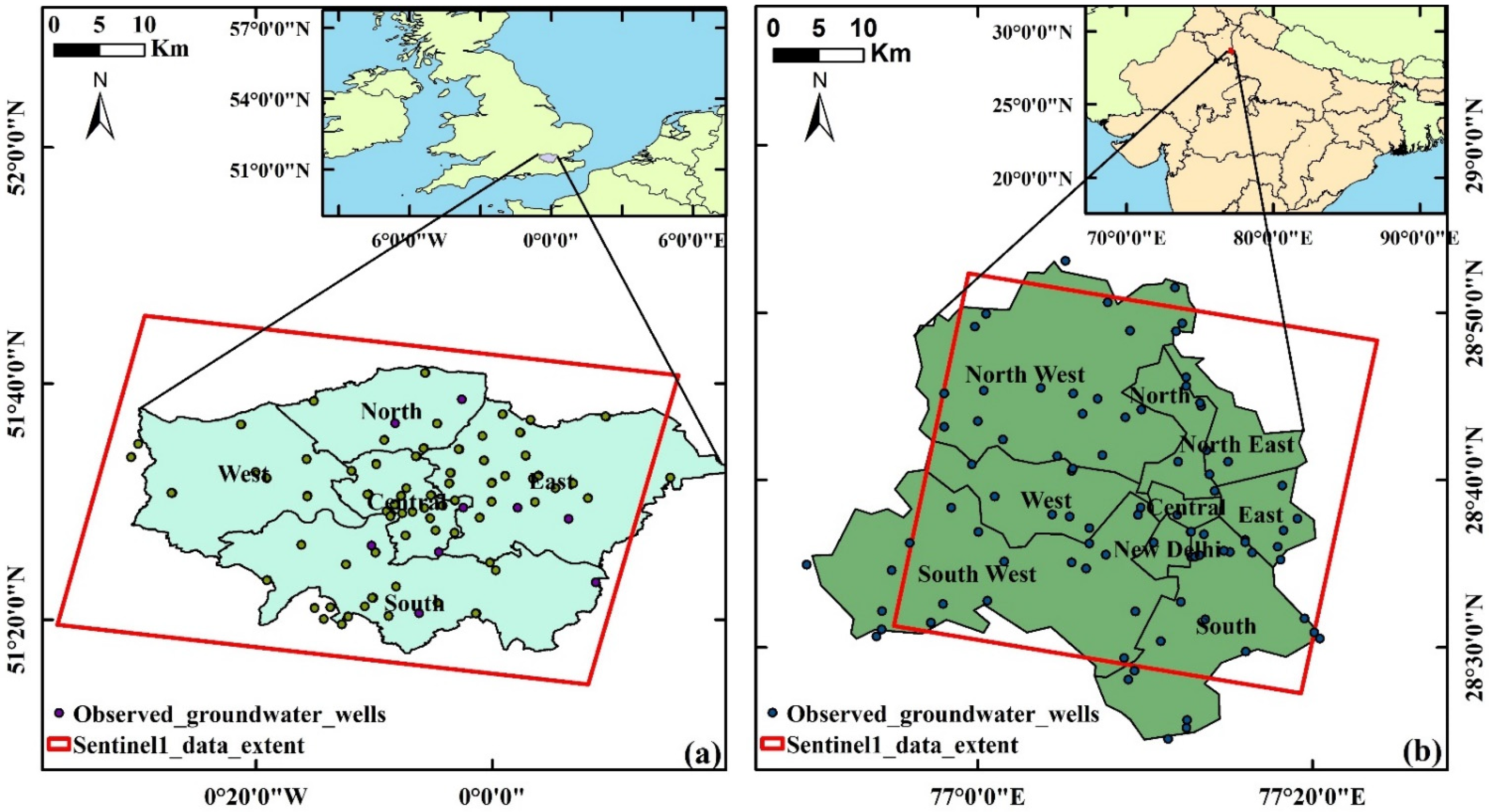
2. Study Area
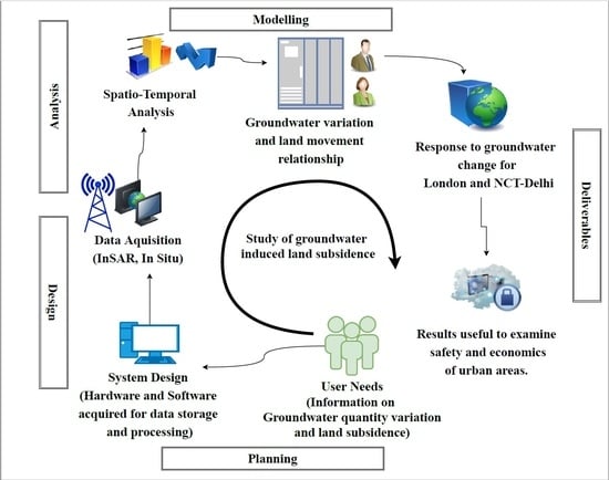
3. Materials and Methods
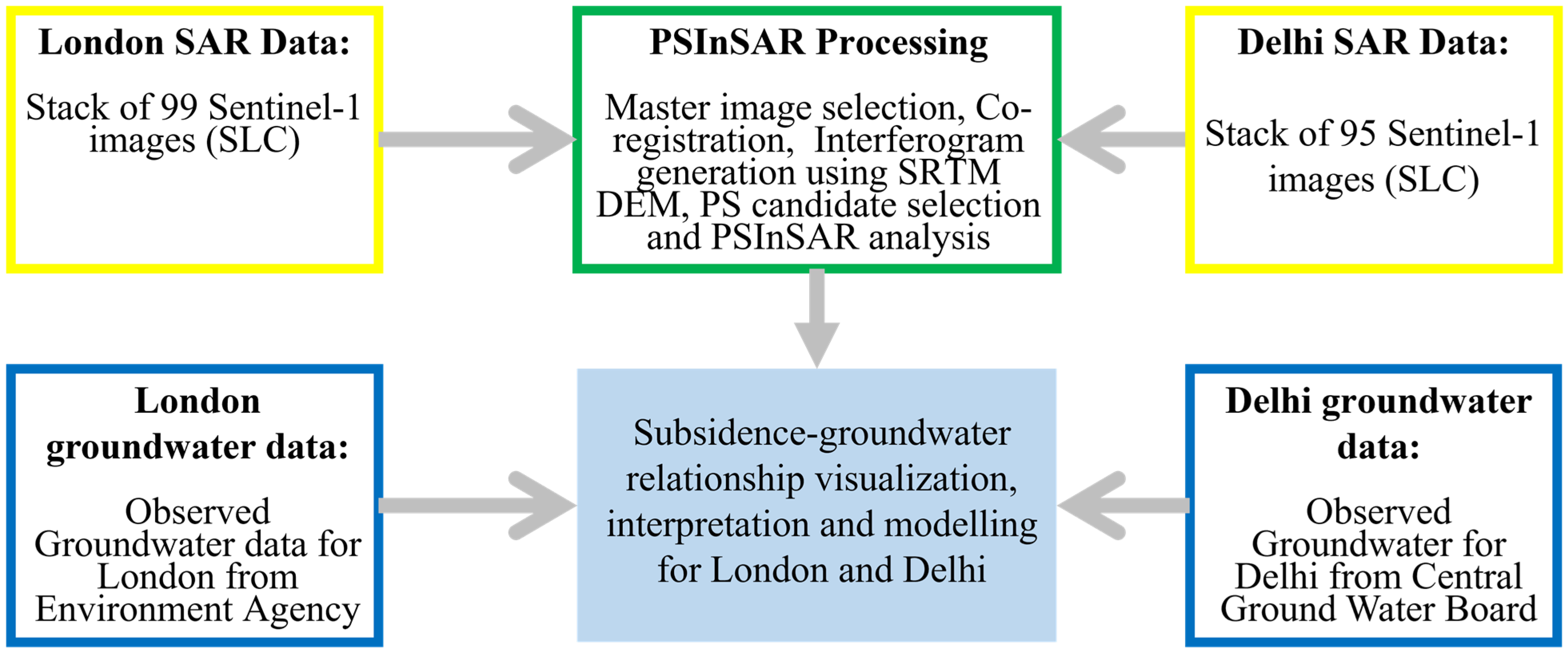
3.1. PSInSAR Processing

| Data | London | NCT-Delhi |
|---|---|---|
| InSAR Data | 99 Sentinel-1 SLC images | 95 Sentinel-1 SLC images |
| VV polarisation, Frame 422, Descending, IW Beam mode | VV polarisation, Frame 496, Descending, IW Beam mode | |
| Resolution: Azimuth: 20 m by Range: 5 m | Resolution: Azimuth: 20 m by Range: 5 m | |
| Repeat Cycle: 12 days | Repeat Cycle: 12 days | |
| Wavelength: 5.6 cm, C-band | Wavelength: 5.6 cm, C-band | |
| Master Image: 1 November 2018 | Master Image: 24 September 2018 | |
| Time period: October 2016 to October 2020 | Time period: October 2016 to October 2020 | |
| Digital Elevation Model: SRTM V4 | Digital Elevation Model: SRTM V4 | |
| Software Used: ENVI SARscape, ArcGIS (ArcMap 10.2.2) | Software Used: ENVI SARscape, ArcGIS (ArcMap 10.2.2) | |
| Ancillary data | Borehole groundwater data from the UK Environment Agency for 81 boreholes. | Groundwater level data (Source: Central Ground Water Board, CGWB) for 98 boreholes. Geological data of Delhi (Source: CGWB) |

3.2. Groundwater Variation
3.3. Groundwater-Subsidence Mathematical Model
| Location | Formation | Thickness (m) | Void Ratio | Porosity | Compression Index |
|---|---|---|---|---|---|
| Delhi | Clay and Kankar | 160 | 0.65 | - | 0.045 |
| Silt and Kankar | 45 | 0.55 | - | 0.0924 | |
| Sand | 20 | 0.45 | - | 0.00525 | |
| London | Lambeth Group | 11.98 | - | 0.35 | 0.0025 |
| Thanet Sands | 10.20 | - | 0.3 | 0.0015 | |
| Chalk Group | 201.09 | - | 0.55 | 0.001 |
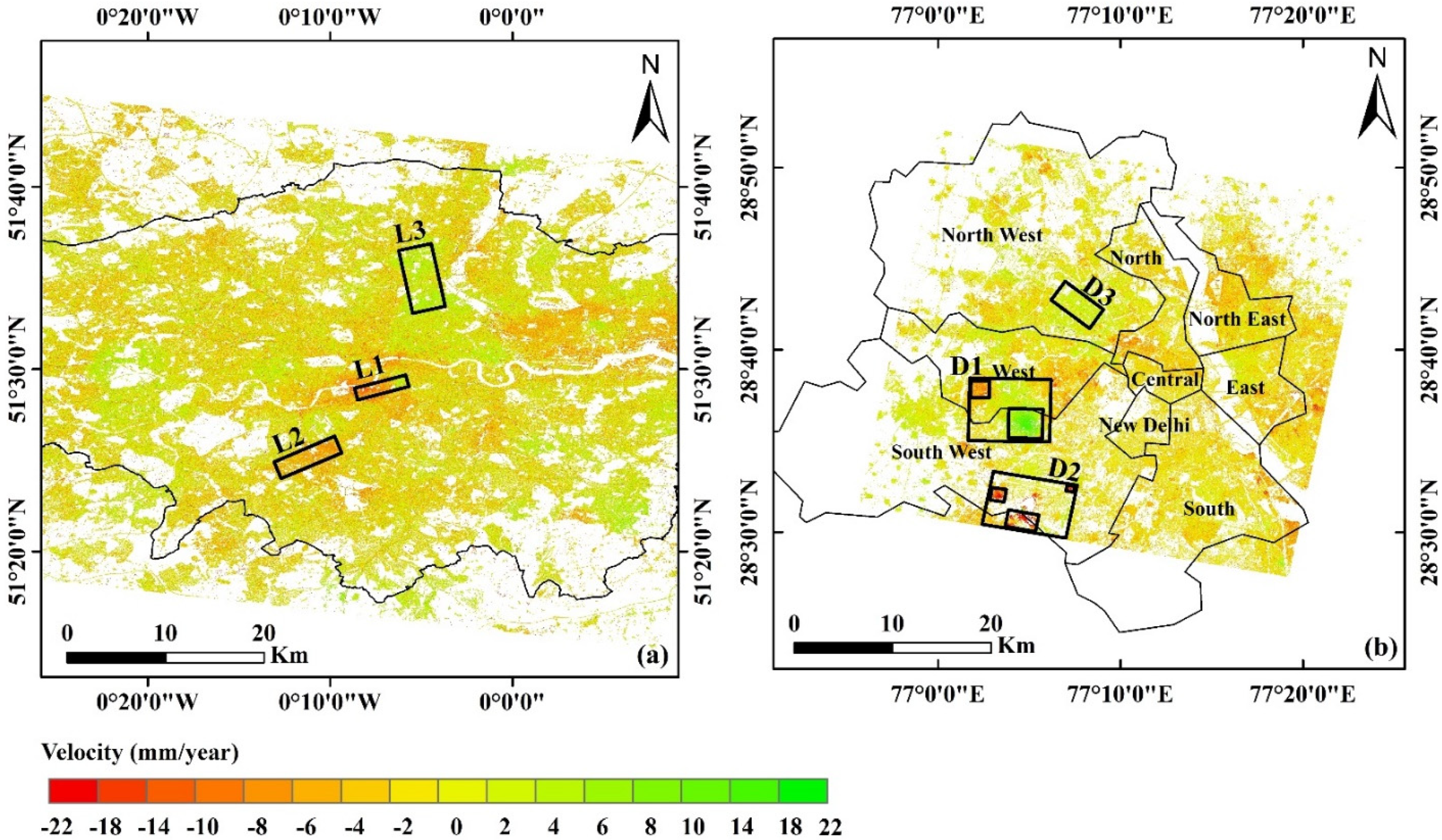
4. Results

| Area | Time-Period | Area (km2) | PS Coherence Threshold Used | Number of Permanent Scatterers Obtained (PS) | PS Density (PS/km2) | Mean Rate of Deformation (mm/Year) | Standard Deviation (mm/Year) |
|---|---|---|---|---|---|---|---|
| London | October 2016 to October 2020 | 2607 | 0.5 | 14,327,370 | 5496 | −0.08 | 1.34 |
| NCT-Delhi | October 2016 to October 2020 | 1611 | 0.5 | 7,764,180 | 4819 | −0.04 | 1.70 |
| Area | Groundwater Monthly Change (m/Month) | Model Change (mm/Year) | PSInSAR Change (mm/Year) | Difference in Rate (Model-PSInSAR) | |
|---|---|---|---|---|---|
| L1 | L1-a | −0.339 | −3.18 | −3.44 | 0.26 |
| L1-b | 0.313 | 2.94 | 4.55 | −1.61 | |
| D1 | D1-a | −0.029 | −7.79 | −5.09 | -2.7 |
| D1-b | 0.038 | 10.14 | 11.06 | −0.92 | |
| L2 | −0.401 | −3.75 | −4.87 | 1.12 | |
| D2 | D2-a | −8.770 | −8.77 | −5.28 | −3.49 |
| D2-b | −0.012 | −3.19 | −4.37 | 1.18 | |
| D2-c | −0.022 | −5.97 | −3.74 | −2.23 | |
| L3 | 0.145 | 1.36 | 3.64 | −2.28 | |
| D3 | 0.041 | 11.13 | 6.30 | 4.83 | |
5. Discussion
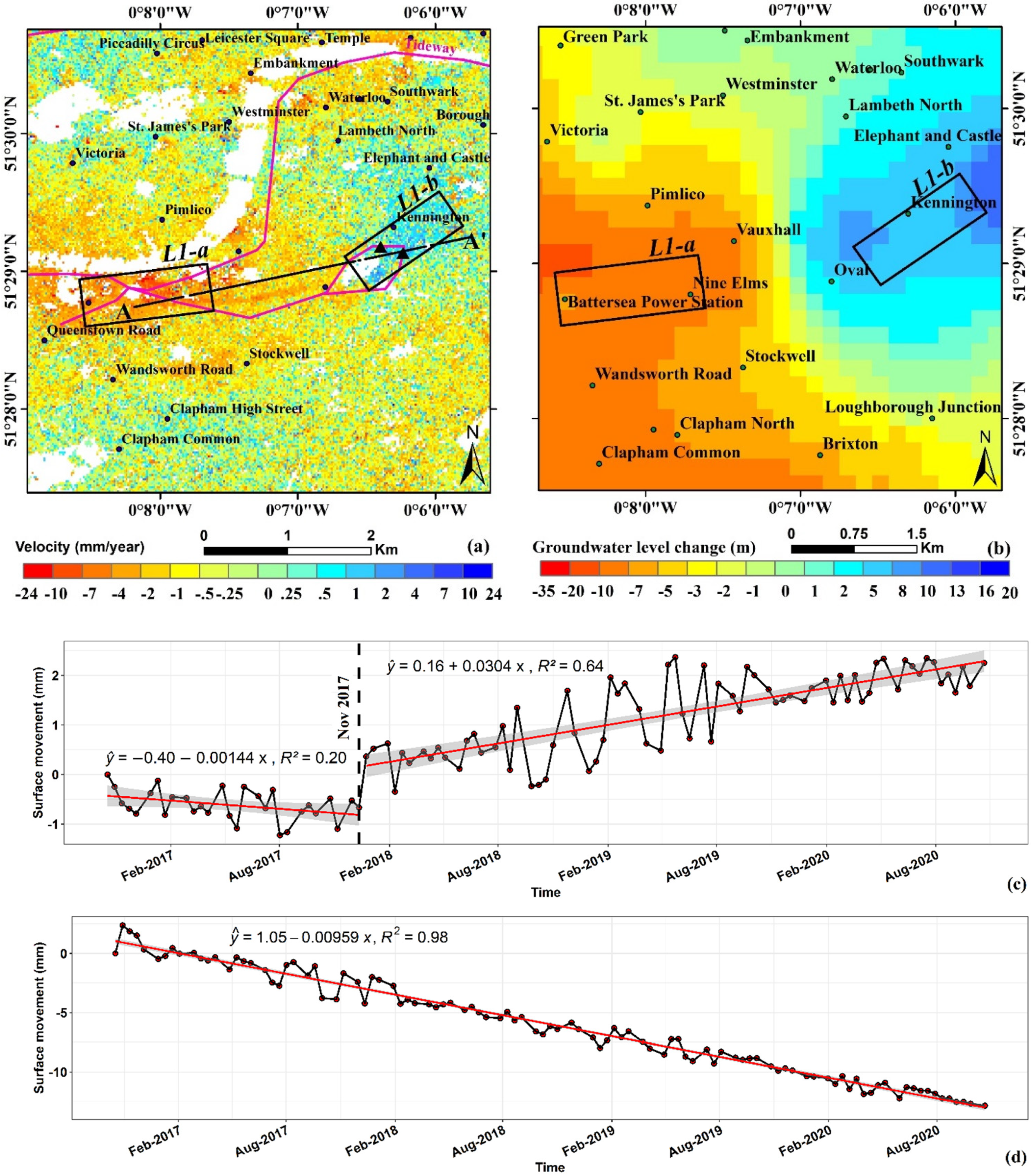
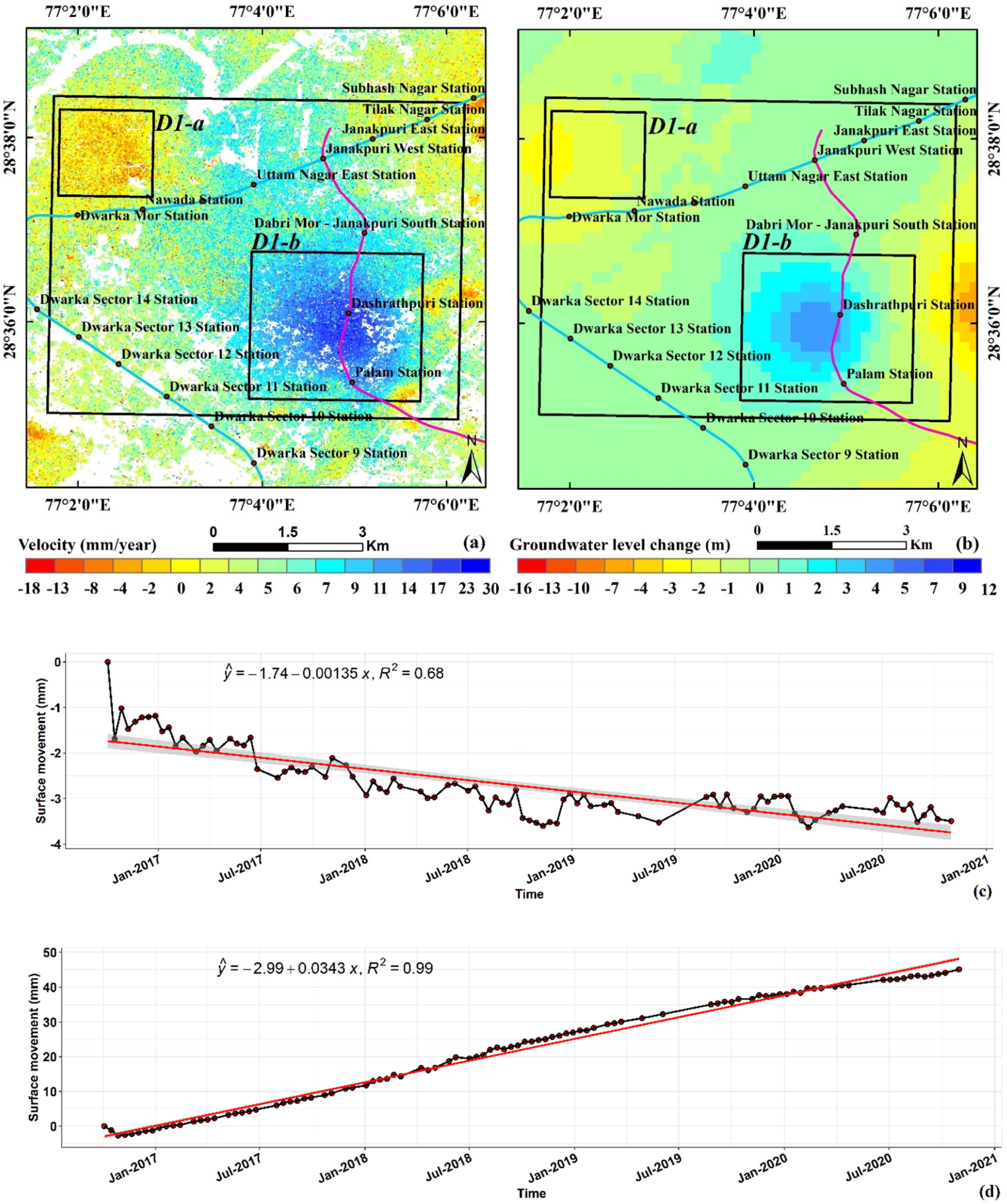
5.1. Differential Land Motion Areas
| Location ID | Location Name | Area (km2) | No. of PS | PS Density (PS/km2) | Land Deformation (mm/Year) | Groundwater Change (m) | |||||
|---|---|---|---|---|---|---|---|---|---|---|---|
| Max | Min | Mean | St. Dev. | Max | Min | Mean | |||||
| L1-a | NLE: Battersea | 0.68 | 7831 | 11,516 | 17.04 | −22.71 | −6.05 | 2.42 | −9.40 | −5.70 | −8.15 |
| L1-b | NLE: Kennington | 0.54 | 6360 | 11,778 | 9.93 | −10.26 | 4.55 | 1.37 | 10.61 | 6.20 | 7.52 |
| D1-a | Magenta-Blue metro line: a | 2.86 | 36,930 | 12,912 | 30.15 | −18.49 | −5.09 | 3.31 | −2.32 | −0.52 | −1.38 |
| D1-b | Magenta-Blue metro line: b | 8.96 | 107,198 | 11,964 | 30.21 | −18.69 | 11.06 | 4.61 | +4.80 | −1.16 | +1.84 |


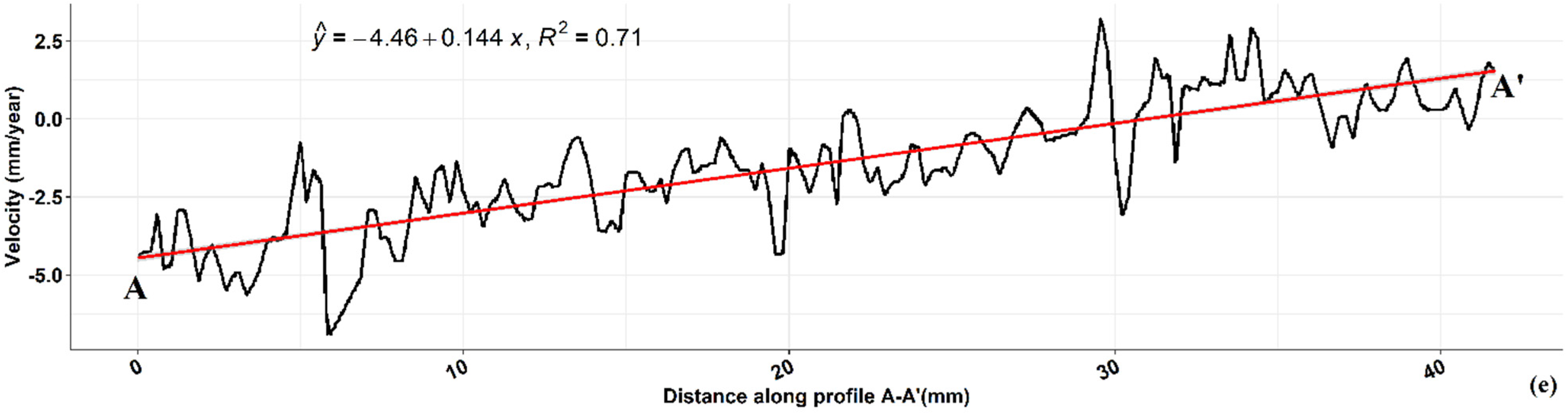
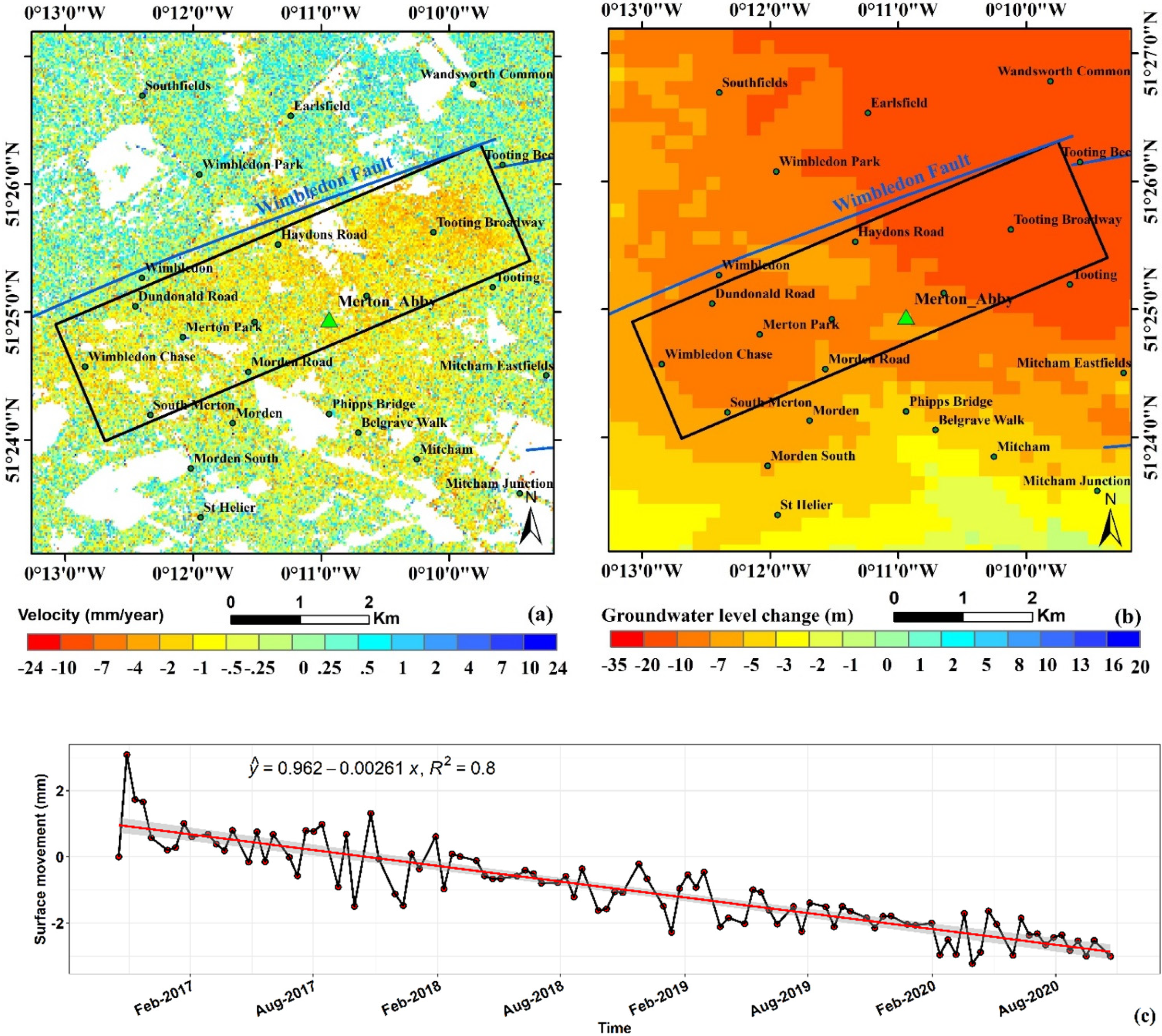
5.2. Subsidence Areas
| Location ID | Location Name | Area (km2) | Number of PS | PS Density (PS/km2) | Land Deformation (mm/Year) | Groundwater Change (m) | |||||
|---|---|---|---|---|---|---|---|---|---|---|---|
| Max | Min | Mean | St. Dev. | Max | Min | Mean | |||||
| L2 | Wimbledon to Tooting | 7.71 | 86,822 | 11,261 | 22.89 | −14.61 | −4.87 | 1.19 | −5.95 | −13.79 | −9.6 |
| D2-a | Delhi-Haryana Border: a | 1.65 | 13,444 | 8148 | 28.43 | −18.71 | −5.28 | 5.26 | −9.46 | −5.97 | −7.77 |
| D2-b | Delhi-Haryana Border: b | 4.70 | 26,368 | 5610 | 30.19 | −18.71 | −4.37 | 7.71 | −7.72 | −4.87 | −5.64 |
| D2-c | Delhi-Haryana Border: c | 0.40 | 4653 | 11,632 | 28.01 | −18.71 | −3.74 | 6.63 | −1.46 | −0.73 | −1.06 |


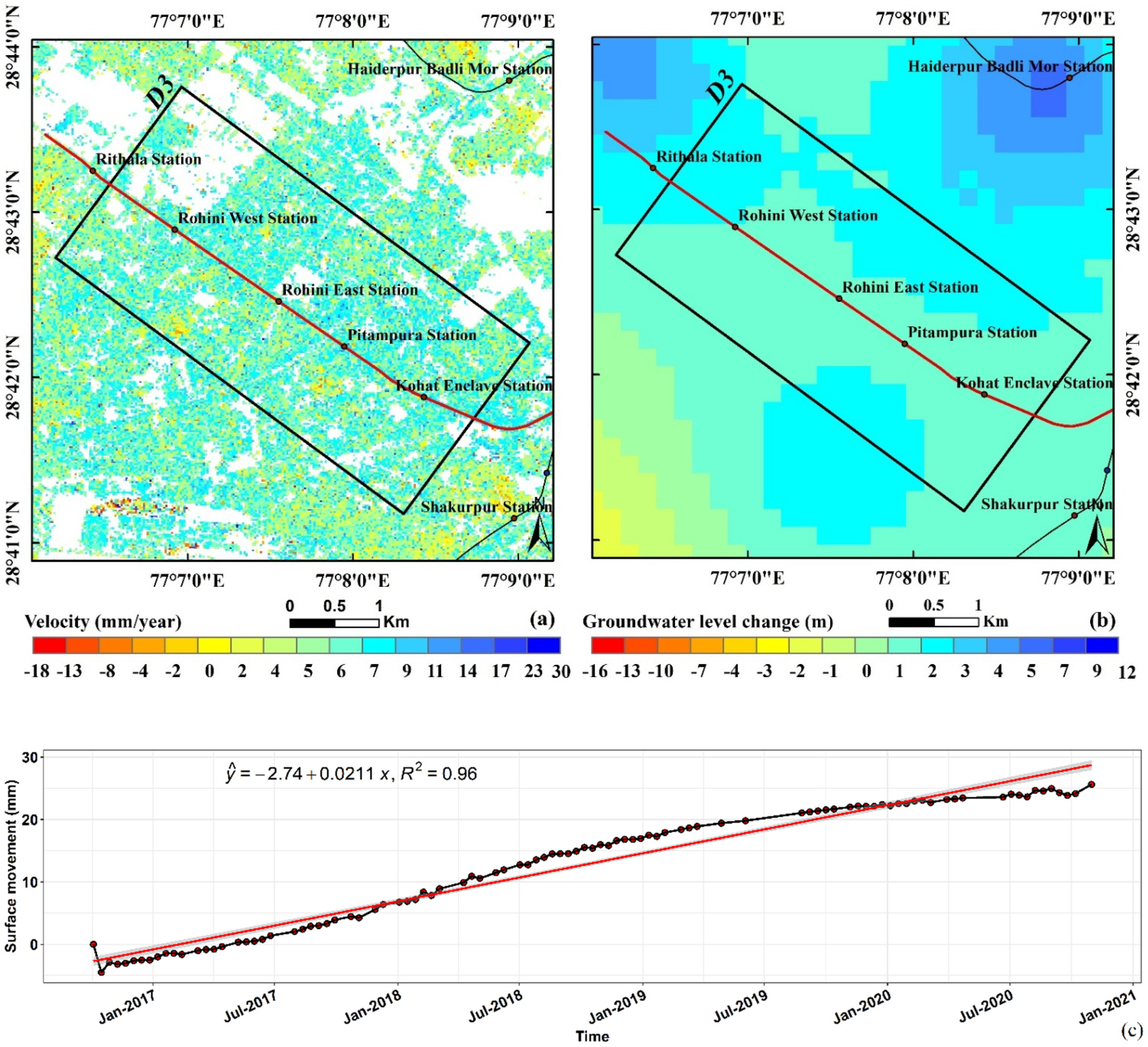
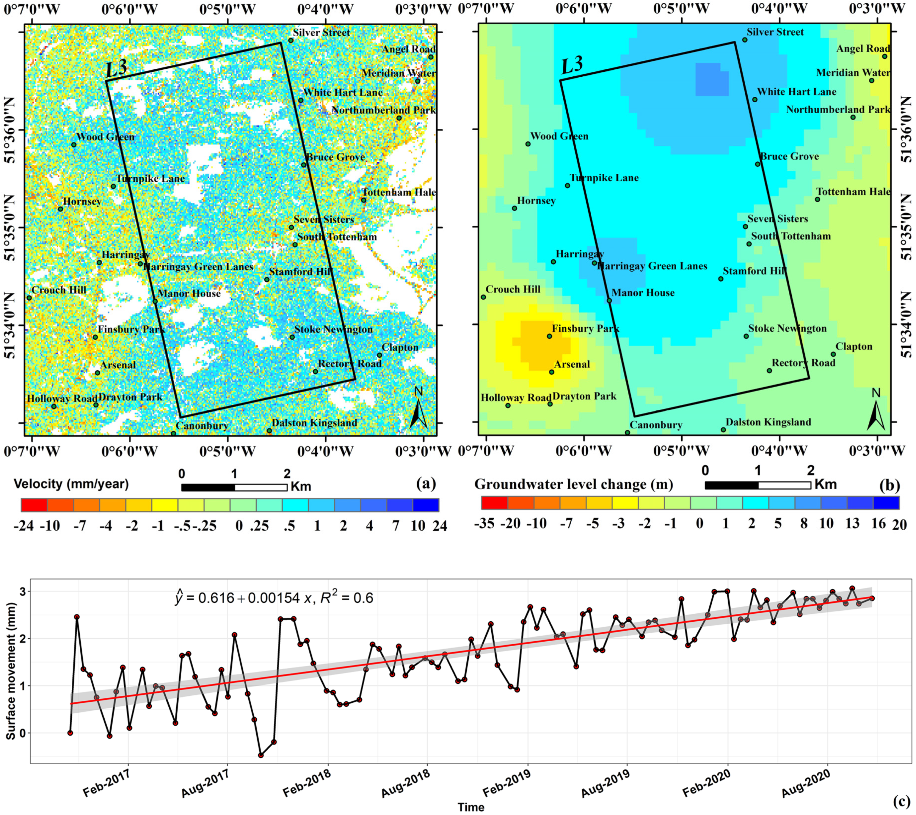
5.3. Uplift Areas
| Location ID | Location Name | Area (km2) | Number of PS | PS Density (PS/km2) | Land Deformation (mm/Year) | Groundwater Change (m) | |||||
|---|---|---|---|---|---|---|---|---|---|---|---|
| Max | Min | Mean | St. Dev. | Max | Min | Avg | |||||
| L3 | Bruce Castle to Clissold Park | 13.8 | 150,354 | 10,895 | 23.09 | −20.54 | 3.64 | 1.21 | 8.28 | −0.04 | 3.48 |
| D3 | Rohini | 10.1 | 99,665 | 9867 | 29.49 | −18.14 | 6.30 | 2.17 | 1.50 | 2.58 | 1.97 |

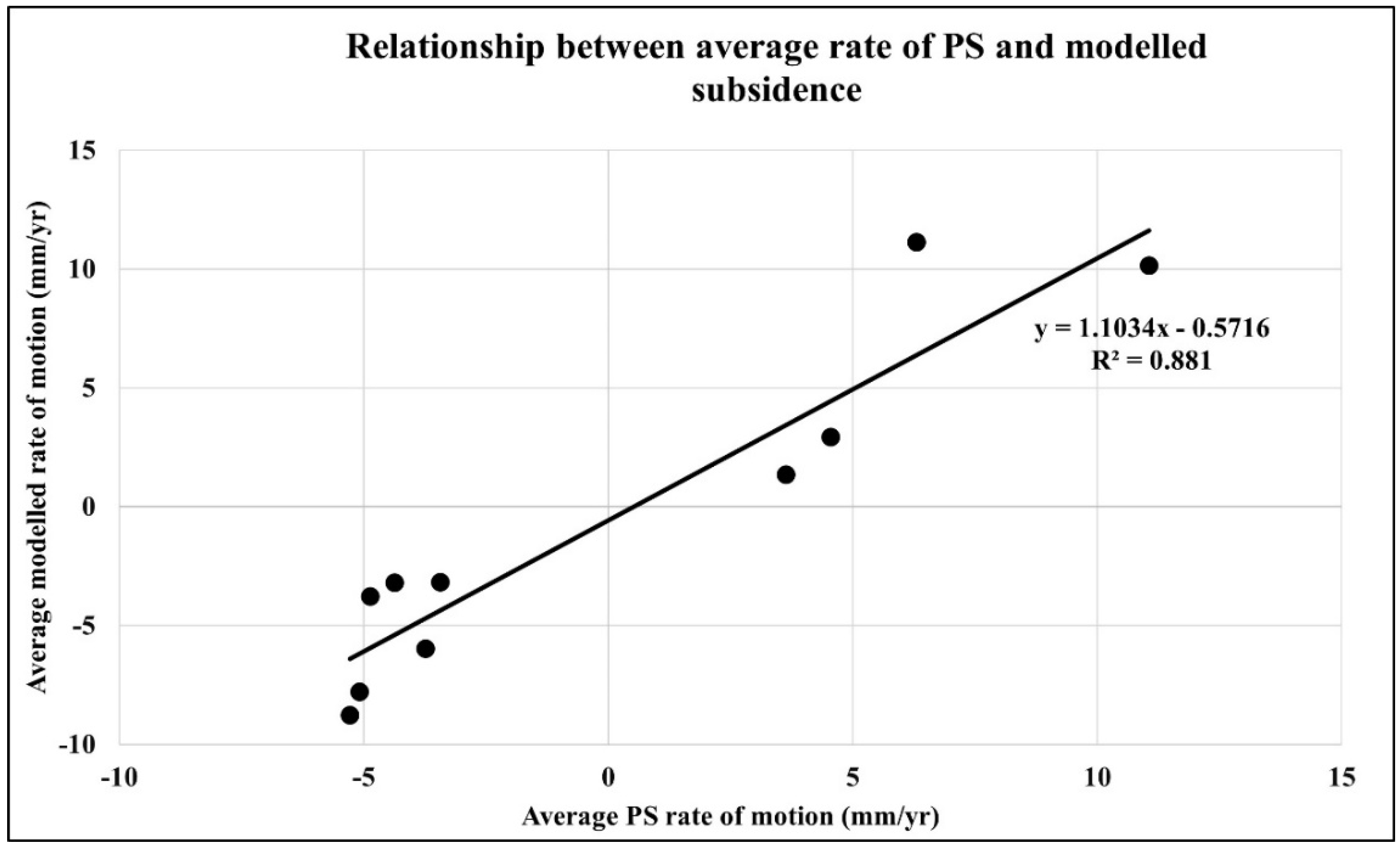
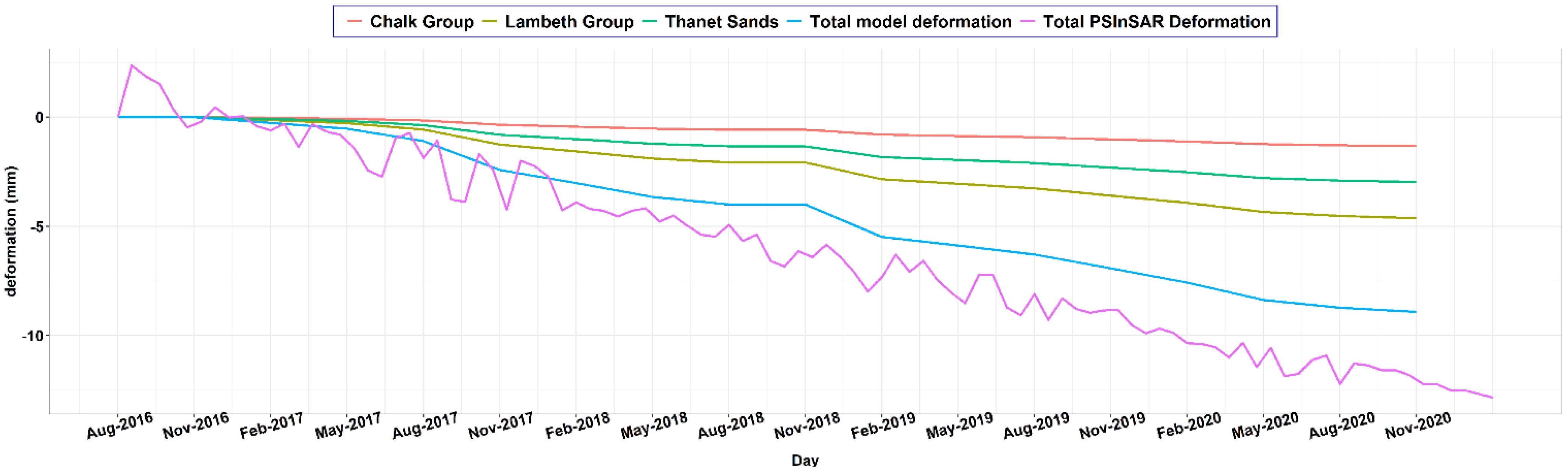
5.4. Modelling of Land Deformation due to Groundwater Change

6. Conclusions
Author Contributions
Funding
Acknowledgments
Conflicts of Interest
References
- Dalin, C.; Wada, Y.; Kastner, T.; Puma, Y.W.M.J. Groundwater depletion embedded in international food trade. Nature 2017, 543, 700–704. [Google Scholar] [CrossRef] [Green Version]
- Wada, Y.; Van Beek, L.P.H.; Van Kempen, C.M.; Reckman, J.W.T.M.; Vasak, S.; Bierkens, M.F.P. Global depletion of groundwater resources. Geophys. Res. Lett. 2010, 37, 37. [Google Scholar] [CrossRef] [Green Version]
- Konikow, L.F.; Kendy, E. Groundwater depletion: A global problem. Hydrogeol. J. 2005, 13, 317–320. [Google Scholar] [CrossRef]
- Li, M.-G.; Chen, J.-J.; Xu, Y.-S.; Tong, D.-G.; Cao, W.-W.; Shi, Y.-J. Effects of groundwater exploitation and recharge on land subsidence and infrastructure settlement patterns in Shanghai. Eng. Geol. 2021, 282, 105995. [Google Scholar] [CrossRef]
- Figueroa-Miranda, S.; Vargas, J.T.; Ramos-Leal, J.A.; Madrigal, V.M.H.; Villaseñor-Reyes, C.I. Land subsidence by groundwater over-exploitation from aquifers in tectonic valleys of Central Mexico: A review. Eng. Geol. 2018, 246, 91–106. [Google Scholar] [CrossRef]
- Zhang, Y.-Q.; Wang, J.-H.; Li, M.-G. Effect of dewatering in a confined aquifer on ground settlement in deep excavations. Int. J. Géoméch. 2018, 18, 04018120. [Google Scholar] [CrossRef]
- Zheng, G.; Ha, D.; Zeng, C.; Cheng, X.; Zhou, H.; Cao, J. Influence of the opening timing of recharge wells on settlement caused by dewatering in excavations. J. Hydrol. 2019, 573, 534–545. [Google Scholar] [CrossRef]
- Lyu, H.-M.; Shen, S.-L.; Zhou, A.; Yang, J. Risk assessment of mega-city infrastructures related to land subsidence using improved trapezoidal FAHP. Sci. Total Environ. 2020, 717, 135310. [Google Scholar] [CrossRef] [PubMed]
- Chai, J.C.; Shen, S.L.; Zhu, H.H.; Zhang, X.L. Land subsidence due to groundwater drawdown in Shanghai. Geotechnique 2004, 54, 143–147. [Google Scholar] [CrossRef]
- Bateson, L.B.; Barkwith AK, A.P.; Hughes, A.G.; Aldiss, D.T. Terrafirma: London H-3 modelled product: Comparison of PS data with the results of a groundwater abstraction related subsidence model. Br. Geol. Surv. Comm. Rep. 2009, 32, 4–47. Available online: http://nora.nerc.ac.uk/id/eprint/8581/1/OR09032.pdf (accessed on 12 July 2021).
- Yu, H.; Gong, H.; Chen, B.; Liu, K.; Gao, M. Analysis of the influence of groundwater on land subsidence in Beijing based on the geographical weighted regression (GWR) model. Sci. Total Environ. 2020, 738, 139405. [Google Scholar] [CrossRef] [PubMed]
- Galloway, D.L.; Burbey, T.J. Review: Regional land subsidence accompanying groundwater extraction. Hydrogeol. J. 2011, 19, 1459–1486. [Google Scholar] [CrossRef]
- Scoular, J.; Ghail, R.; Mason, P.J.; Lawrence, J.; Bellhouse, M.; Holley, R.; Morgan, T. Retrospective InSAR analysis of east london during the construction of the Lee tunnel. Remote Sens. 2020, 12, 849. [Google Scholar] [CrossRef] [Green Version]
- Agarwal, V.; Kumar, A.; Gomes, R.L.; Marsh, S. Monitoring of ground movement and groundwater changes in London using InSAR and GRACE. Appl. Sci. 2020, 10, 8599. [Google Scholar] [CrossRef]
- Biswas, K.; Chakravarty, D.; Mitra, P.; Misra, A. Spatial-correlation based persistent scatterer interferometric study for ground deformation. J. Indian Soc. Remote Sens. 2017, 45, 913–926. [Google Scholar] [CrossRef]
- Peltier, A.; Bianchi, M.; Kaminski, E.; Komorowski, J.-C.; Rucci, A.; Staudacher, T. PSInSAR as a new tool to monitor pre-eruptive volcano ground deformation: Validation using GPS measurements on Piton de la Fournaise. Geophys. Res. Lett. 2010, 37. [Google Scholar] [CrossRef]
- Kim, J.-S.; Kim, D.-J.; Kim, S.-W.; Won, J.-S.; Moon, W.M. Monitoring of urban land surface subsidence using PSInSAR. Geosci. J. 2007, 11, 59–73. [Google Scholar] [CrossRef]
- Karanam, V.; Motagh, M.; Garg, S.; Jain, K. Multi-sensor remote sensing analysis of coal fire induced land subsidence in Jharia Coalfields, Jharkhand, India. Int. J. Appl. Earth Obs. Geoinf. 2021, 102, 102439. [Google Scholar] [CrossRef]
- Ferretti, A.; Prati, C.; Rocca, F. Nonlinear subsidence rate estimation using permanent scatterers in differential SAR interferometry. IEEE Trans. Geosci. Remote Sens. 2000, 38, 2202–2212. [Google Scholar] [CrossRef] [Green Version]
- Mason, P.J.; Ghail, R.C.; Bischoff, C.; Skipper, J.A. Detecting and Monitoring Small-Scale Discrete Ground Movements Across London, Using Persistent SCATTERER InSAR (PSI); ICE Publishing: London, UK, 2015. [Google Scholar]
- Khorrami, M.; Alizadeh, B.; Tousi, E.G.; Shakerian, M.; Maghsoudi, Y.; Rahgozar, P. How groundwater level fluctuations and geotechnical properties lead to asymmetric subsidence: A PSInSAR Analysis of land deformation over a transit corridor in the Los Angeles Metropolitan area. Remote Sens. 2019, 11, 377. [Google Scholar] [CrossRef] [Green Version]
- Khorrami, M.; Abrishami, S.; Maghsoudi, Y.; Alizadeh, B.; Perissin, D. Extreme subsidence in a populated city (Mashhad) detected by PSInSAR considering groundwater withdrawal and geotechnical properties. Sci. Rep. 2020, 10, 1–16. [Google Scholar]
- Devleeschouwer, X.; Declercq, P.Y.; Flamion, B.; Brixko, J.; Timmermans, A.; Vanneste, J. Uplift revealed by radar interferometry around Liège (Belgium): A relation with rising mining groundwater. In Proceedings of the Post-Mining Symposium, Nancy, France, 6–8 February 2008; pp. 6–8. [Google Scholar]
- Jones, M.A.; Hughes, A.; Jackson, C.; Van Wonderen, J.J. Groundwater resource modelling for public water supply management in London. Geol. Soc. Lond. Spéc. Publ. 2012, 364, 99–111. [Google Scholar] [CrossRef] [Green Version]
- EA. Management of the London BAsin Chalk Aquifer; Environment Agency: Bristol, UK, 2019. [Google Scholar]
- Central Ground Water Board. Ground Water Year Book-India 2017–2018; Ministry of Water Resources, River Development and Ganga Rejuvenation: New Delhi, India, 2018. [Google Scholar]
- Central Ground Water Board. Ground Water Year Book, NCT Delhi, 2015–2016; Central Ground Water Board: Kolkata, India, 2016. [Google Scholar]
- Gupte, P.R. Groundwater Resources vs Domestic Water Demand and Supply-NCT Delhi; Central Ground Water Board: Kolkata, India, 2019. [Google Scholar]
- Garg, S.; Motagh, M.; Jayaluxmi, I. Land Subsidence in Delhi, India investigated using Sentinel-1 InSAR measurements. In Proceedings of the EGU General Assembly 2020, Online, 4–8 May 2020. [Google Scholar] [CrossRef]
- Ford, J.R.; Mathers, S.J.; Royse, K.; Aldiss, D.T.; Morgan, D.J. Geological 3D modelling: Scientific discovery and enhanced understanding of the subsurface, with examples from the UK. Z. Dtsch. Ges. Für Geowiss. 2010, 161, 205–218. [Google Scholar] [CrossRef] [Green Version]
- Mathers, S.; Burke, H.; Terrington, R.; Thorpe, S.; Dearden, R.; Williamson, J.; Ford, J. A geological model of London and the Thames Valley, southeast England. Proc. Geol. Assoc. 2014, 125, 373–382. [Google Scholar] [CrossRef] [Green Version]
- BGS. Industrial and Urban Pollution of Groundwater; UK Groundwater Forum: Oxfordshire, UK, 2013. [Google Scholar]
- Bonì, R.; Cigna, F.; Bricker, S.; Meisina, C.; McCormack, H. Characterisation of hydraulic head changes and aquifer properties in the London Basin using Persistent Scatterer Interferometry ground motion data. J. Hydrol. 2016, 540, 835–849. [Google Scholar] [CrossRef] [Green Version]
- Central Ground Water Board. Groundwater Scenario in India, November 2016; Central Ground Water Board: Kolkata, India, 2016. [Google Scholar]
- GLA. London Datastore. Greater London Authority (GLA). 2021. Available online: https://data.london.gov.uk/dataset/trend-based-population-projections (accessed on 12 July 2021).
- ESD. Demographic Profile of Delhi, Economic SURVEY of Delhi. 2021. Available online: http://delhiplanning.nic.in/sites/default/files/19.Demography.pdf (accessed on 12 July 2021).
- PS Tutorial. Sarmap SA, Switzerland. 2014. Available online: http://www.sarmap.ch/tutorials/PS_Tutorial_V_0_9.pdf (accessed on 12 July 2021).
- Agarwal, V.; Kumar, A.; Gomes, R.L.; Marsh, S. An overview of SAR sensors and software and a comparative study of poen source (Snap) and commercial (SARscape) software for DInSAR analysis using C-band Radar images. In Proceedings of the 41st Asian Conference on Remote Sensing—ACRS, Deqing, China, 9–11 November 2020; Available online: https://www.researchgate.net/publication/345335178 (accessed on 15 May 2021).
- Simonetto, E.; Follin, J.-M. An overview on interferometric SAR software and a comparison between DORIS and SARSCAPE Packages. In Lecture Notes in Geoinformation and Cartography; Springer: New York, NY, USA, 2012. [Google Scholar]
- Sahraoui, O.H.; Hassaine, B.; Serief, C. Radar Interferometry with Sarscape Software. In Proceedings of the XXIII FIG Congress Munich, Germany, 8–13 October 2006. [Google Scholar]
- Sarmap. SARscape Help Manual. 2014. Available online: http://sarmap.ch/tutorials/Basic.pdf (accessed on 12 July 2021).
- EA. Management of the London Basin Chalk Aquifer. Status Report 2017; Environ. Agency: Bristol, UK, 2017. Available online: https://www.gov.uk/government/publications/london-basin-chalk-aquifer-annual-status-report (accessed on 12 July 2021).
- Bartier, P.M.; Keller, C. Multivariate interpolation to incorporate thematic surface data using inverse distance weighting (IDW). Comput. Geosci. 1996, 22, 795–799. [Google Scholar] [CrossRef]
- Gee, D.; Bateson, L.; Grebby, S.; Novellino, A.; Sowter, A.; Wyatt, L.; Marsh, S.; Morgenstern, R.; Athab, A. Modelling groundwater rebound in recently abandoned coalfields using DInSAR. Remote Sens. Environ. 2020, 249, 112021. [Google Scholar] [CrossRef]
- Terzaghi, K. Principles of soil mechanics, IV—Settlement and consolidation of clay. Eng. News-Rec. 1925, 95, 874–878. [Google Scholar]
- Shearer, T. A numerical model to calculate land subsidence, applied at Hangu in China. Eng. Geol. 1998, 49, 85–93. [Google Scholar] [CrossRef]
- Poland, J.F. Guidebook to Studies of Land Subsidence Due to Ground-Water Withdrawal; UNESCO: Paris, France, 1984. [Google Scholar]
- Zimmerman, R.W. Compressibility of Sandstones; Elsevier: Amsterdam, The Netherlands, 1990. [Google Scholar]
- Sarkar, A.; Ali, S.; Kumar, S.; Shekhar, S.; Rao, S. Groundwater environment in Delhi, India. In Groundwater Environment in Asian Cities; Elsevier: Amsterdam, The Netherlands, 2016; pp. 77–108. [Google Scholar]
- Zheng, M.; Deng, K.; Fan, H.; Du, S. Monitoring and analysis of surface deformation in mining area based on InSAR and GRACE. Remote Sens. 2018, 10, 1392. [Google Scholar] [CrossRef] [Green Version]
- Transport for London, Northern Line Extension—Transport for London. 2021. Available online: https://tfl.gov.uk/travel-information/improvements-and-projects/northern-line-extension (accessed on 4 April 2021).
- DMRC. Delhi Metro Present Projects (DMRC), DMRC Off. Website. 2021. Available online: http://www.delhimetrorail.com/projectpresent.aspx (accessed on 21 July 2021).
- DMRC. Annual Report of DMRC 2017–2018. 2018. Available online: http://www.delhimetrorail.com/annual_report.aspx/ (accessed on 12 July 2021).
- BGS. Geoindex Onshore for Boreholes Provided by British Geological Survey. 2021. Available online: http://mapapps2.bgs.ac.uk/geoindex/home.html?layer=BGSBoreholes (accessed on 5 May 2021).
- Aldiss, D. The Stratigraphical Framework for the Palaeogene Successions of the London Basin, UK; British Geography Survey: Nottingham, UK, 2014. [Google Scholar]
- Geoiq. GeoIQ’s Spatial AI: India’s Comprehensive and Granular Location Data Stack, Geoiq. 2021. Available online: https://geoiq.io/ (accessed on 2 April 2021).
- E.P. 7. 3. 3. 778. Google, Delhi Haryana Border. 28°30’54.84” N, 77°4’21.80” E, Eye alt 13.45 km. Borders and labels; Places Layers. NOAA, DigitalGlobe 2021, Google Earth. Available online: http://www.google.com/earth/index.html (accessed on 10 July 2021).
- Mammen, S.S. Delhi’s Most Expensive and Posh Residential Areas. Available online: https://housing.com/news/posh-residential-areas-in-delhi/ (accessed on 20 September 2021).
Publisher’s Note: MDPI stays neutral with regard to jurisdictional claims in published maps and institutional affiliations. |
© 2021 by the authors. Licensee MDPI, Basel, Switzerland. This article is an open access article distributed under the terms and conditions of the Creative Commons Attribution (CC BY) license (https://creativecommons.org/licenses/by/4.0/).
Share and Cite
Agarwal, V.; Kumar, A.; Gee, D.; Grebby, S.; Gomes, R.L.; Marsh, S. Comparative Study of Groundwater-Induced Subsidence for London and Delhi Using PSInSAR. Remote Sens. 2021, 13, 4741. https://doi.org/10.3390/rs13234741
Agarwal V, Kumar A, Gee D, Grebby S, Gomes RL, Marsh S. Comparative Study of Groundwater-Induced Subsidence for London and Delhi Using PSInSAR. Remote Sensing. 2021; 13(23):4741. https://doi.org/10.3390/rs13234741
Chicago/Turabian StyleAgarwal, Vivek, Amit Kumar, David Gee, Stephen Grebby, Rachel L. Gomes, and Stuart Marsh. 2021. "Comparative Study of Groundwater-Induced Subsidence for London and Delhi Using PSInSAR" Remote Sensing 13, no. 23: 4741. https://doi.org/10.3390/rs13234741
APA StyleAgarwal, V., Kumar, A., Gee, D., Grebby, S., Gomes, R. L., & Marsh, S. (2021). Comparative Study of Groundwater-Induced Subsidence for London and Delhi Using PSInSAR. Remote Sensing, 13(23), 4741. https://doi.org/10.3390/rs13234741