Article

Deep Learning Triplet Ordinal Relation Preserving Binary Code for Remote Sensing Image Retrieval Task

1
School of Computer Science and Technology, Shandong University of Technology, Zibo 255000, China
2
Key Laboratory of Symbolic Computation and Knowledge Engineering of Ministry of Education, Jilin University, Changchun 130012, China
3
School of Computer Science and Technology, Jilin University, Changchun 130012, China
*
Author to whom correspondence should be addressed.
Remote Sens. 2021, 13(23), 4786; https://doi.org/10.3390/rs13234786
Submission received: 26 September 2021 / Revised: 9 November 2021 / Accepted: 23 November 2021 / Published: 26 November 2021
(This article belongs to the Special Issue Deep Learning and Computer Vision in Remote Sensing)

Abstract

:
As satellite observation technology rapidly develops, the number of remote sensing (RS) images dramatically increases, and this leads RS image retrieval tasks to be more challenging in terms of speed and accuracy. Recently, an increasing number of researchers have turned their attention to this issue, as well as hashing algorithms, which map real-valued data onto a low-dimensional Hamming space and have been widely utilized to respond quickly to large-scale RS image search tasks. However, most existing hashing algorithms only emphasize preserving point-wise or pair-wise similarity, which may lead to an inferior approximate nearest neighbor (ANN) search result. To fix this problem, we propose a novel triplet ordinal cross entropy hashing (TOCEH). In TOCEH, to enhance the ability of preserving the ranking orders in different spaces, we establish a tensor graph representing the Euclidean triplet ordinal relationship among RS images and minimize the cross entropy between the probability distribution of the established Euclidean similarity graph and that of the Hamming triplet ordinal relation with the given binary code. During the training process, to avoid the non-deterministic polynomial (NP) hard problem, we utilize a continuous function instead of the discrete encoding process. Furthermore, we design a quantization objective function based on the principle of preserving triplet ordinal relation to minimize the loss caused by the continuous relaxation procedure. The comparative RS image retrieval experiments are conducted on three publicly available datasets, including UC Merced Land Use Dataset (UCMD), SAT-4 and SAT-6. The experimental results show that the proposed TOCEH algorithm outperforms many existing hashing algorithms in RS image retrieval tasks.

Graphical Abstract

1. Introduction

With the rapid development of satellite observation technology, both the amount and the quality of remote sensing (RS) images have improved dramatically. An era of remote sensing image big data has arrived. An increasing number of researchers are focusing on the task of large-scale RS image retrieval, due to its broad applications, such as disaster prevention, soil erosion monitoring, disaster rescue scenario and short-term weather forecasting [1,2,3,4,5]. The content-based image retrieval (CBIR) [6,7] method extracts feature information representing RS image content and finds similar RS images by comparing the distance values among their feature information. However, the feature information in CBIR is always represented as high dimensional float point data and it is difficult to directly compute the similarity relationship based on the original high dimensional feature information. Fortunately, hashing methods [1,2,3,4,5,8,9] can map high dimensional float point data into compact binary codes and return the approximate nearest neighbors according to Hamming distance; this measure effectively improves the retrieval speed. In summary, the content-based image retrieval method assisted by hashing algorithms enables the efficient and effective retrieval of target remote sensing images from a large-scale dataset.
In recent years, many hashing algorithms [10,11,12,13,14] have been proposed to achieve the approximate nearest neighbor (ANN) search task, due to its advantage of computation and storage. According to the learning framework, the existing hashing algorithms can be roughly divided into two types: the shallow model [12,13,14] and the deep model [10,11,15,16]. Conventional shallow hashing algorithms, such as locality sensitive hashing (LSH) [14], spectral hashing (SH) [17], iterative quantization hashing (ITQ) [13] and k-means hashing (KMH) [12], have been applied to various approximate nearest neighbor search tasks, including image retrieval. Locality sensitive hashing [14] is a kind of data-independent method, which learns hashing functions without a training process. LSH [14] randomly generates linear hashing functions and encodes data into binary codes according to their projection signs. Spectral hashing (SH) [17] utilizes a spectral graph to represent the similarity relationship among data points. The binary codes in SH are generated by partitioning a spectral graph. Iterative quantization hashing [13] considers the vertexes of a hyper cubic as encoding centers. ITQ [13] rotates the principal component analysis (PCA) projected data and maps the rotated data to the nearest encoding center. The encoding centers in ITQ are fixed and they are not adaptive to the data distribution [12]. To fix this problem, k-means hashing [12] learns the encoding centers by simultaneously minimizing the quantization error and the similarity loss. KMH [12] encodes the data as the same binary code as the nearest center. For the image search task, the shallow model first learns the high dimensional features, such as scale-invariant feature transform (SIFT) [18] or a holistic representation of the spatial envelope (GIST) [19], then retrieves similar images by mapping these features into the compact Hamming space. In contrast, the deep learning model enables end-to-end representation learning and hash coding [10,11,20,21,22]. In particular, the deep learning to hash, such as deep Cauchy hashing (DCH) [11] and twin-bottleneck hashing (TBH) [10], proves crucial to jointly learn, thereby similarly preserving the representations and control quantization error of converting continuous representations to binary codes. Deep Cauchy hashing [11] defines a pair-wise similarity preserving restriction based on Cauchy distribution and it heavily penalizes the similar image pairs with large Hamming distance. Twin-bottleneck hashing [10] proposes a code-driven graph to represent the similarity relationship among data points and aims to minimize the loss between the original data and decoded data. These deep learning to hash methods have shown state-of-the-art results for many datasets.
Recently, many hashing algorithms have been applied to the large-scale RS image search task [1,2,3,4,5]. Partial randomness hashing [23] maps RS images into a low dimensional Hamming space by both the random and well-trained projection functions. Demir et al. [24] proposed two kernel-based methods to learn hashing functions in the kernel space. Liu et al. [25] fully utilized the supervised deep learning framework and hashing learning to generate the binary codes of RS images. Li et al. [25] carried out a comprehensive study of DHNN systems and aimed to introduce the deep neural network into the large-scale RS image search task. Fan et al. [26] proposed a distribution consistency loss (DCL) to capture the intra-class distribution and inter-class ranking. Both deep Cauchy hashing [11] and the distribution consistency loss functions [26] employ pairwise similarity [15] to describe the relationship among data. However, the similarity relationship among RS images is more complex. In this paper, we propose the triplet ordinal cross entropy hashing (TOCEH) to deal with the large-scale RS image search task. The flowchart of the proposed TOCEH is shown in Figure 1.
As shown in Figure 1, the TOCEH algorithm consists of two parts: the triplet ordinal tensor graph generation part and the hash code learning part. In part 1, we first utilize the AlexNet [27] pre-trained on the ImageNet dataset [28] to extract the 4096-dimension image feature information of the target domain RS images. Then, we separately compute the similarity and dissimilarity graph among the high dimensional features. Finally, we establish the triplet ordinal tensor graph representing the ordinal relation among any triplet RS images. Part 2 utilizes two fully connected layers to generate binary codes. During the training process, we define two excellent objection functions, including the triplet ordinal cross entropy loss and the triplet ordinal quantization loss to guarantee the performance of the obtained binary codes and utilize the back-propagation mechanism to optimize the variables of the deep neural network. The main contributions of the proposed TOCEH are summarized as follows:
1.
The learning procedure of TOCEH takes into account the triplet ordinal relations, rather than the pairwise or point-wise similarity relations, which can enhance the performance of preserving the ranking orders of approximate nearest neighbor retrieval results from the high dimensional feature space to the Hamming space.
2.
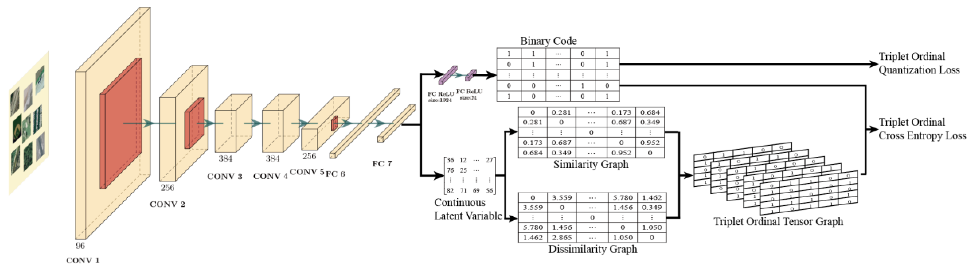
TOCEH establishes a triplet ordinal graph to explicitly indicate the ordinal relationship among any triplet RS images and preserves the ranking orders by minimizing the inconsistency between the probability distribution of the given triplet ordinal relation and that of the ones derived from binary codes.
3.
We conduct comparative experiments on three RS image datasets: UCMD, SAT-4 and SAT-6. Extensive experimental results demonstrate that TOCEH generates highly concentrated and compact hash codes, and it outperforms some existing state-of-the-art hashing methods in large-scale RS image retrieval tasks.
The rest of this paper is organized as follows. Section 2 introduces the proposed TOCEH algorithm. Section 2.1 shows the important notation. The hash learning problem is stated in Section 2.2. The tensor graph representing the triplet ordinal relation among RS images is introduced in Section 2.3. We provide the formulation of triplet ordinal cross entropy loss and triplet ordinal quantization loss in Section 2.4 and Section 2.5, respectively. The extensive experimental evaluations are presented in Section 3. Finally, we set out a conclusion in Section 4.

2. Triplet Ordinal Cross Entropy Hashing

2.1. Notation

In this paper, we use the letters B and X to separately represent the data matrix in the Hamming and Euclidean spaces. The columns in the data matrix are denoted as the letters with subscript. The important notations are summarized in Table 1.

2.2. Hashing Learning Problem

The purpose of the hashing algorithm [3,10,11] is to learn the hashing function H(∙), mapping the high dimensional float point data x into the compact Hamming space as defined in Equation (1). B(x) represents the compact binary code of x.
B ( x ) = ( s i g n ( H ( x ) 0.5 ) + 1 ) / 2
With the assistance of the obtained hashing function H(∙), we can encode RS image content as compact binary code and efficiently achieve RS image search task according to their Hamming distances [1,2,3,4,5,23,24,25]. Furthermore, to guarantee the quality of the RS image search result, we expect the triplet ordinal relation among RS images in the Hamming space to be consistent with that in the original space [29,30]. To illustrate this requirement, a simple example is provided below. Here, xi, xj and xk separately represent RS image content information. In the original space, the image pair (xi, xj) is more similar than the image pair (xj, xk). After mapping them into the Hamming space, the Hamming distance of the data pair (xi, xj) should be smaller than that of the data pair (xj, xk). This constraint is defined as in Equation (2).
| | H ( x i ) H ( x j ) | | 1 | | H ( x k ) H ( x j ) | | 1 s . t . | | x i x j | | 2 2 | | x k x j | | 2 2
The constraint in Equation (2) guarantees that the ranking order of the retrieval result in the Hamming space is consistent with that in the Euclidean space. Thus, the hashing algorithm, satisfying the triplet ordinal relation preserving constraint, can achieve RS image ANN search tasks [31,32,33,34,35].

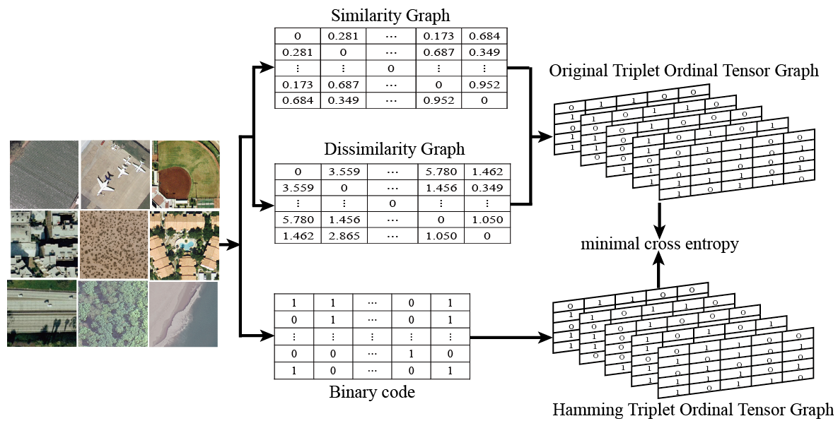
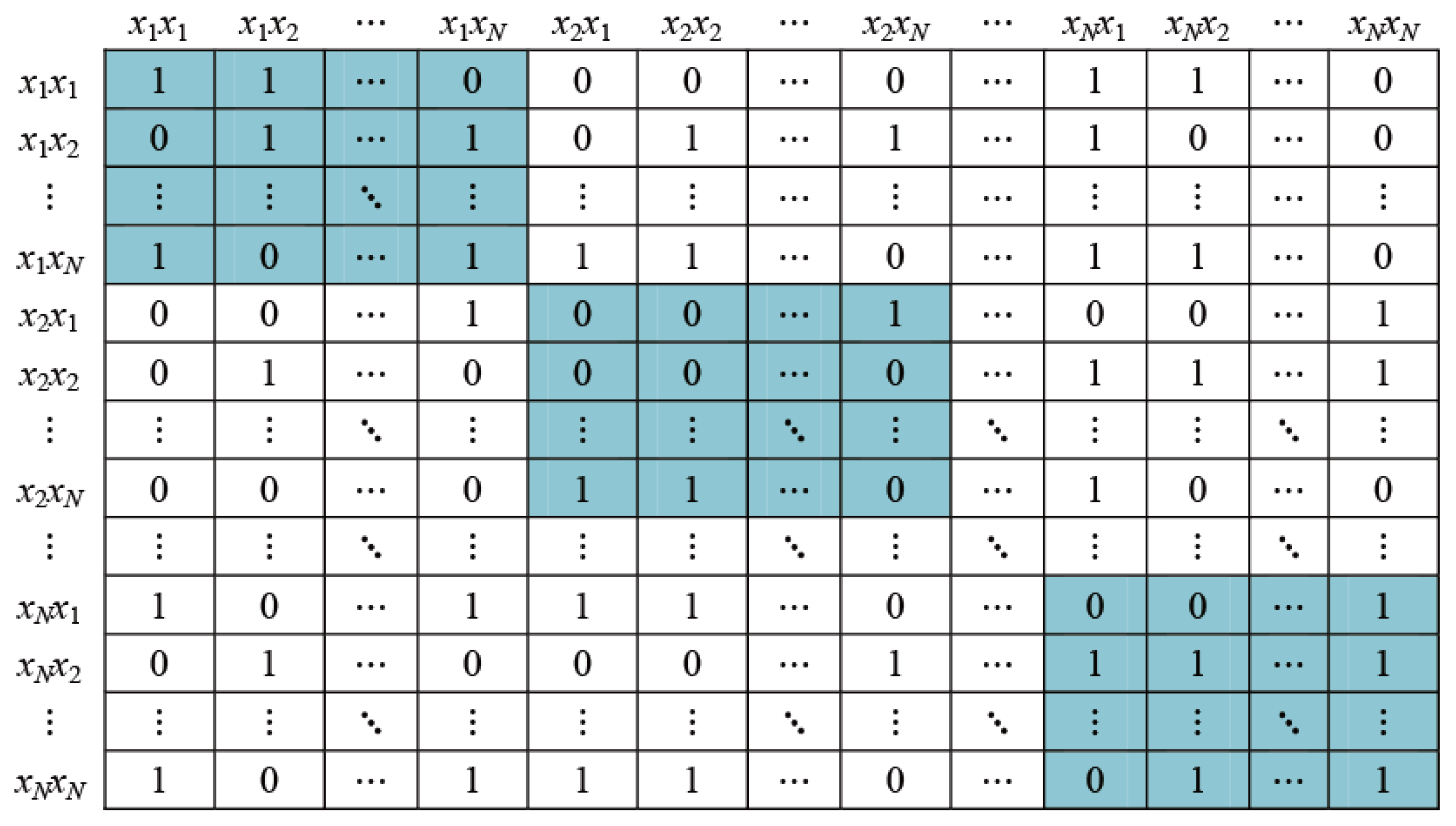
2.3. Triplet Ordinal Tensor Graph

To learn the triplet ordinal relation preserving hashing functions, the first problem is how to efficiently compute the probability distribution of the triplet ordinal relation among the training set in the original space.
Generally, we select the triplet data (xi, xj, xk) from the training set to compute their ordinal relation, where the data pair (xi, xj) has a small Euclidean distance value and (xj, xk) is considered as the dissimilar data pair. However, this mechanism needs to randomly select triplet samples and compare the distance values among all data points. It has a high time complexity and costly memory. Furthermore, it is difficult to define the similar and dissimilar data pairs for the problem without supervised information.
In this paper, to solve the above problem, we employ a tensor ordinal graph G to represent the ordinal relation among the triplet images (xi, xj, xk). We establish the tensor ordinal graph G by tensor production and each entry in G is calculated as G(ij, jk) = S(i, j)∙DS(j, k). S(i, j) is the similarity graph as defined in Equation (3). A larger value of S(i, j) means the data pair (xi, xj) is more similar. DS(i, j) is the dissimilarity graph and its value is calculated as DS(i, j) = 1/S(i, j).
S ( i , j ) = { 0 , i = j e | | x i x j | | 2 2 / 2 σ 2 , o t h e r w i s e
We further process G to obey the binary distribution as in Equation (4). gijk is the entry of G(i, j, k).
{ g i j k = 1 , G ( i , j , k ) > 1 g i j k = 0 , G ( i , j , k ) 1
Given N training samples, the size of the similarity graph and dissimilarity graph is N × N. The tensor product of the two graphs is shown in Figure 2, and its size is N 2 × N 2. However, the proposed TOCEH only concerns the relative similarity relationship among the data pairs (xi, xj) and (xj, xk). The corresponding elements are marked blue. There are N rectangles and each rectangle contains N × N elements. We pick up these elements and restore them into a matrix with the size of N × N × N.
Finally, the ordinal relation among any triplet items can be represented by the triplet ordinal graph G, as defined in Equation (5).
{ S ( i , j ) > S ( k , j ) , g i j k = 1 S ( i , j ) S ( k , j ) , g i j k = 0
To illustrate the cases defined in Equation (5), a simple explanation is provided below. For the triplet item (xi, xj, xk), the value of the (ij, kj)-th entry is G(ij, kj) = S(i, j)∙DS(k, j) = S(i, j)/S(k, j). If the triplet ordinal relation is S(i, j) > S(k, j), we have G(ij, kj) > 1 and gijk = 1; otherwise, we have G(ij, kj) ≤ 1 and gijk = 0. Thus, the value in G can correctly indicate the true ordinal relation among any triplet items.
As described above, we can establish a tensor ordinal graph G with size N3 to represent the triplet ordinal relation among N images. In practice, during the training procedure, we use L (LN) k-means centers to establish the tensor ordinal graph, which can reduce the training time complexity.

2.4. Triplet Ordinal Cross Entropy Loss

In this section, we define Ĝ as RS images’ triplet ordinal relation in the Hamming space. As discussed in Section 2.2, an ideal hashing algorithm should minimize the inconsistency between Ĝ and G. In this paper, the above requirement is achieved by minimizing the cross entropy value, as defined in Equation (6).
min C E H ( G , G ) = min P ( G ) log P ( G )
P(G) defined in Equation (7) computes the probability distribution of RS images’ triplet ordinal relation in the Euclidean space.
{ w i j k = T 1 T g i j k = 1 w i j k = T 0 T g i j k = 0
The definitions of T1, T0 and T are shown in Equation (8). T1 is the number of samples with a value of 1 in the matrix G and T0 is the number of samples with a value of 0 in the matrix G. T is the total number of the elements in the matrix G.
T 1 = i , j , k = 1 N g i , j , k T 0 = i , j , k = 1 N ( 1 g i , j , k ) T = i , j , k = 1 N | 2 g i , j , k 1 |
P(Ĝ) is a conditional probability of the triplet ordinal relation with given binary codes. As the samples are independent from each other, we calculate P(Ĝ) by Equation (9).
P ( G ) = Π i , j , k = 1 N P ( g i j k | B i , B j , B k )
P(gijk|Bi, Bj, Bk) is the probability of the triplet images satisfying the ordinal relation gijk, and the samples’ are assigned the binary codes (Bi, Bj, Bk). The definition is shown in Equation (10).
P ( g i j k | B i , B j , B k ) = { ϕ ( d h ( B k , B j ) d h ( B i , B j ) ) , g i j k = 1 1 ϕ ( d h ( B k , B j ) d h ( B i , B j ) ) , g i j k = 0
We further rewrite the definition of P(gijk|Bi, Bj, Bk) as in Equation (11).
P ( g i j k | B i , B j , B k ) = ϕ ( d h ( B k , B j ) d h ( B i , B j ) ) g i j k ( 1 ϕ ( d h ( B k , B j ) d h ( B i , B j ) ) ) 1 g i j k
dh(∙,∙) returns the Hamming distance and ϕ(∙) computes the probability value. If gijk = 1, the probability value should be close to 1 as dh(Bk, Bj)-dh(Bi, Bj) gets larger and the probability value should be close to 0 as dh(Bk, Bj)-dh(Bi, Bj) gets smaller. The characteristic of the function (∙) is shown in Figure 3.
In this paper, the sigmoid function is considered as the function (∙) as in Equation (12).
ϕ ( d h ( B k , B j ) d h ( B i , B j ) ) = 1 1 + e α ( d h ( B k , B j ) d h ( B i , B j ) )
By merging Equations (7), (9), (11) and (12) into Equation (6), we reach the final triplet ordinal relation preserving objective function, as shown in Equation (13).
L = w i j k log Π i , j , k = 1 N P ( g i j k | B i , B j , B k ) = i , j , k = 1 N w i j k log P ( s i j k | B i , B j , B k ) = i , j , k = 1 N w i j k log ( 1 1 + e α ( d h ( B k , B j ) d h ( B i , B j ) ) ) g i j k ( 1 1 1 + e α ( d h ( B k , B j ) d h ( B i , B j ) ) ) 1 g i j k ) = i , j , k = 1 N w i j k ( g i j k log ( 1 + e α ( d h ( B k , B j ) d h ( B i , B j ) ) ) + ( 1 g i j k ) log ( 1 + 1 e α ( d h ( B k , B j ) d h ( B i , B j ) ) ) ) = i , j , k = 1 N w i j k ( g i j k log ( e α ( d h ( B k , B j ) d h ( B i , B j ) ) ) + log ( 1 + 1 e α ( d h ( B k , B j ) d h ( B i , B j ) ) ) )

2.5. Triplet Ordinal Quantization Loss

Generally, the sign function is adopted to map the real-valued data output by the last layer of deep neural network into binary codes. However, it generates discrete values and makes the objective function non-deterministic polynomial (NP) hard for optimization [20,36]. To fix this problem, the continuous tanh(⋅) function is utilized instead of the sign(⋅) function in this paper. Furthermore, to minimize the quantization loss caused by the continuous relaxation procedure, we expect the output of the tanh(⋅) function to be close to ±1. Here, we utilize the triplet ordinal cross entropy to formulate the quantization loss. We define the binary code obtained by the tanh(⋅) function as Bitah. Bref is the reference binary code. The ideal encoding result is 1. Thus, we formulate the quantization loss Q as in Equation (14).
Q = i = 1 N log P ( 1 | ( | | B t a h i | | , 1 , | | B r e f | | ) ) = i = 1 N log ϕ ( d h ( | | B t a h i | | , 1 ) + δ ) = i = 1 N log ( 1 + e α ( d h ( | | B t a h i | | , 1 ) + δ ) )
In Equation (14), the triplet ordinal relation among (||Bitah ||, 1 and ||Bref||) is defined as 1 and it indicates that the data pair (||Bitah ||, 1) is more similar than the data pair (1, ||Bref||). Therefore, to minimize the quantization loss, the Hamming distance of the data pair (||Btah||, 1) should be smaller than the Hamming distance δ = dh(||Bref||, 1). During the training procedure, we tune the value of δ to balance the optimization complexity and the approximation performance. A small δ value let the encoding results be close to the output of sign function and the training process will become hard. In contrast, a large δ value creates low optimization complexity, but it leads to poor approximation results.
After applying the continuous relaxation mechanism, we compute the Hamming distance of one data pair by Equation (15). ⨂ computes the sum of bitwise production value. f8(⋅) represents the output of the deep neural network’s last layer.
d h ( B i , B j ) = 1 2 ( M tanh ( f 8 ( x i ) ) tanh ( f 8 ( x j ) ) )
Finally, we utilize the back propagation mechanism to optimize the variables of the deep neural network by simultaneously minimizing the triplet ordinal relation cross entropy loss in Equation (13) and the quantization loss in Equation (14).

3. Experimental Setting and Results

In this section, we introduce the comparative experimental setting and evaluate the approximate nearest neighbor search performance of the proposed TOCEH and some state-of-the-art hashing methods.

3.1. Datasets

The comparative experiments are conducted on three large-scale RS image datasets, including UC Merced land use dataset (UCMD) [37], SAT-4 dataset [38] and SAT-6 dataset [38]. The details of these three RS image datasets are introduced below.
1.
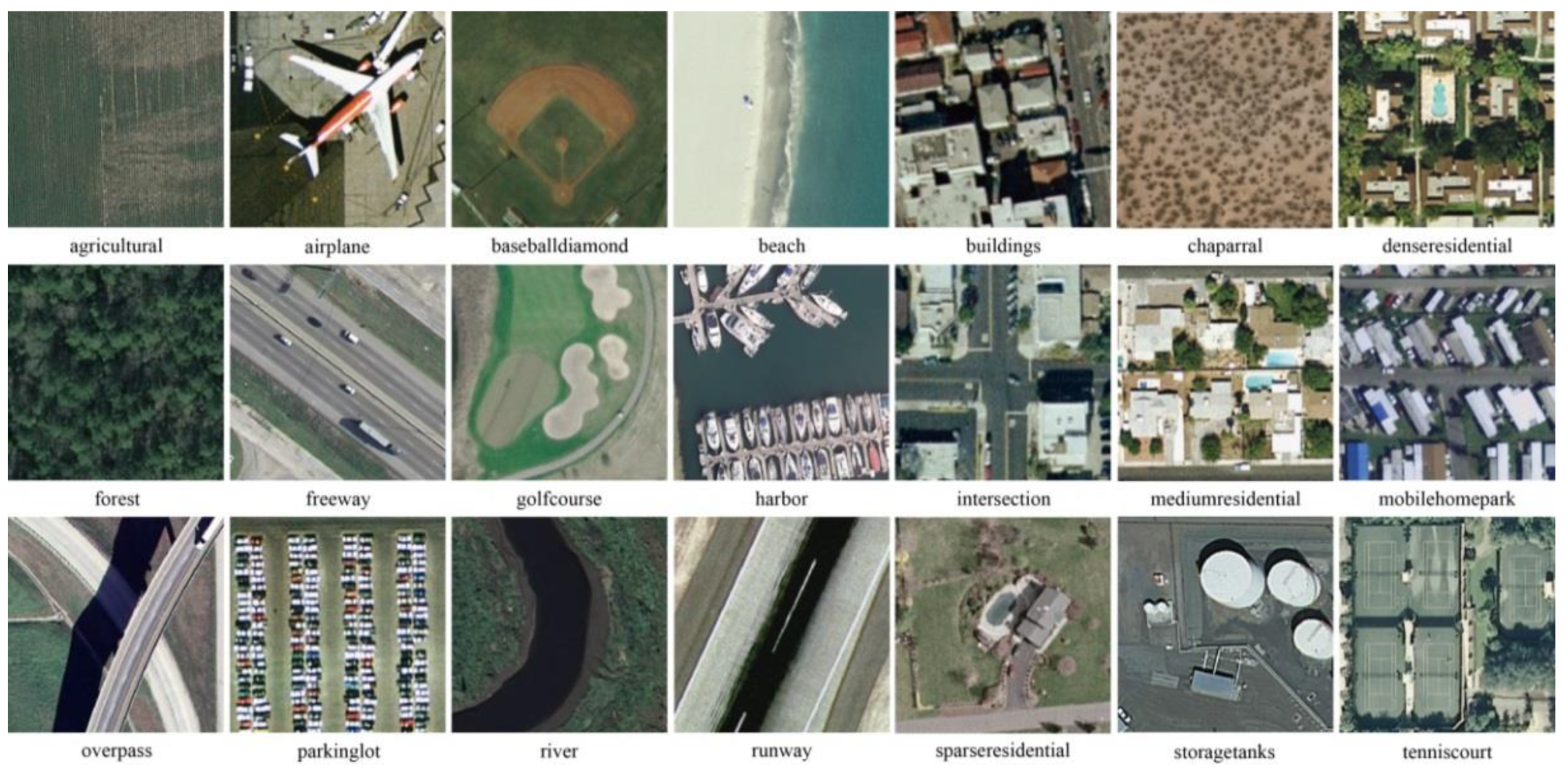
UCMD [37] stores aerial image scenes with a human label. There are 21 land cover categories, and each category includes 100 images with the normalized size of 256 × 256 pixels. The spatial resolution of each pixel is 0.3 m. We randomly choose 420 images as query samples and the remaining 1680 images are utilized as training samples.
2.
The total number of images in SAT-4 [38] is 500k and it includes four broad land cover classes: barren land, grass land, trees and other. The size of images is normalized to 28 × 28 pixels and the spatial resolution of each pixel is 1 m. We randomly select 400k images to train the network and the other 100k images to test the ANN search performance.
3.
The SAT-6 [38] dataset contains 405k images covering barren land, buildings, grassland, roads, trees and water bodies. These images are normalized to 28 × 28 pixels size and the spatial resolution of each pixel is 1 m. We randomly select 81k images as query set and the other 324k images as training set.
Some sample images of the above three datasets are shown in Figure 4, Figure 5 and Figure 6, and the statistics are summarized in Table 2.

3.2. Experimental Settings and Evaluation Matrix

To verify the ANN search performance of the proposed TOCEH method, many state-of-the-art hashing methods, including locality sensitive hashing (LSH) [14], spectral hashing (SH) [17], iterative quantization hashing method (ITQ) [13], k-means hashing (KMH) [12], partial randomness hashing (PRH) [23], deep variational binaries (DVB) [39], deep hashing (DH) [40], DeepBit [41], deep Cauchy hashing (DCH) [11] and twin-bottle neck hashing (TBH) [10] are utilized as the baseline methods. LSH [14], SH [17], ITQ [13] and KMH [12] belong to the shallow methods. During the ANN search experiments, we extract the content information from RS images by AlexNet and the features are represented as 4096-dimension float point data. Then, these shallow hashing methods map the 4096-dimension features into the compact Hamming space and achieve the ANN search task according to the Hamming distance. DCH [11], TBH [10], DVB [39], DH [40], DeepBit [41] and the proposed TOCEH are deep learning hashing methods. They directly generate the RS image’s binary feature using an end-to-end mechanism.
The training process and comparative experiments are conducted on a high-performance computer with GPU Tesla T4 16 GB, CPU Intel Xeon 6242R 3.10 GHz and 64 GB RAM.
To evaluate the ANN search performance, two widely used standards, mean average precision (mAP) and recall curves, are employed in this paper.
The recall curve represents the fraction of the positive samples that are successfully retrieved. The definition of recall is shown in Equation (16). #(⋅) returns the number of samples.
r e c a l l = # ( r e t r i e v e d   p o s i t i v e   s a m p l e s ) # ( a l l   p o s i t i v e   s a m p l e s )
Mean average precision value expresses the return rate of positive samples as defined in Equation (17). |total| is the total number of retrieved samples. Ki returns the number of positive samples of the i-th query sample. rank(j) is the ranking number of the j-th positive sample in the retrieved results.
m A P = 1 | t o t a l | i = 1 | t o t a l | 1 K i j = 1 K i j r a n k ( j )

3.3. Experimental Results

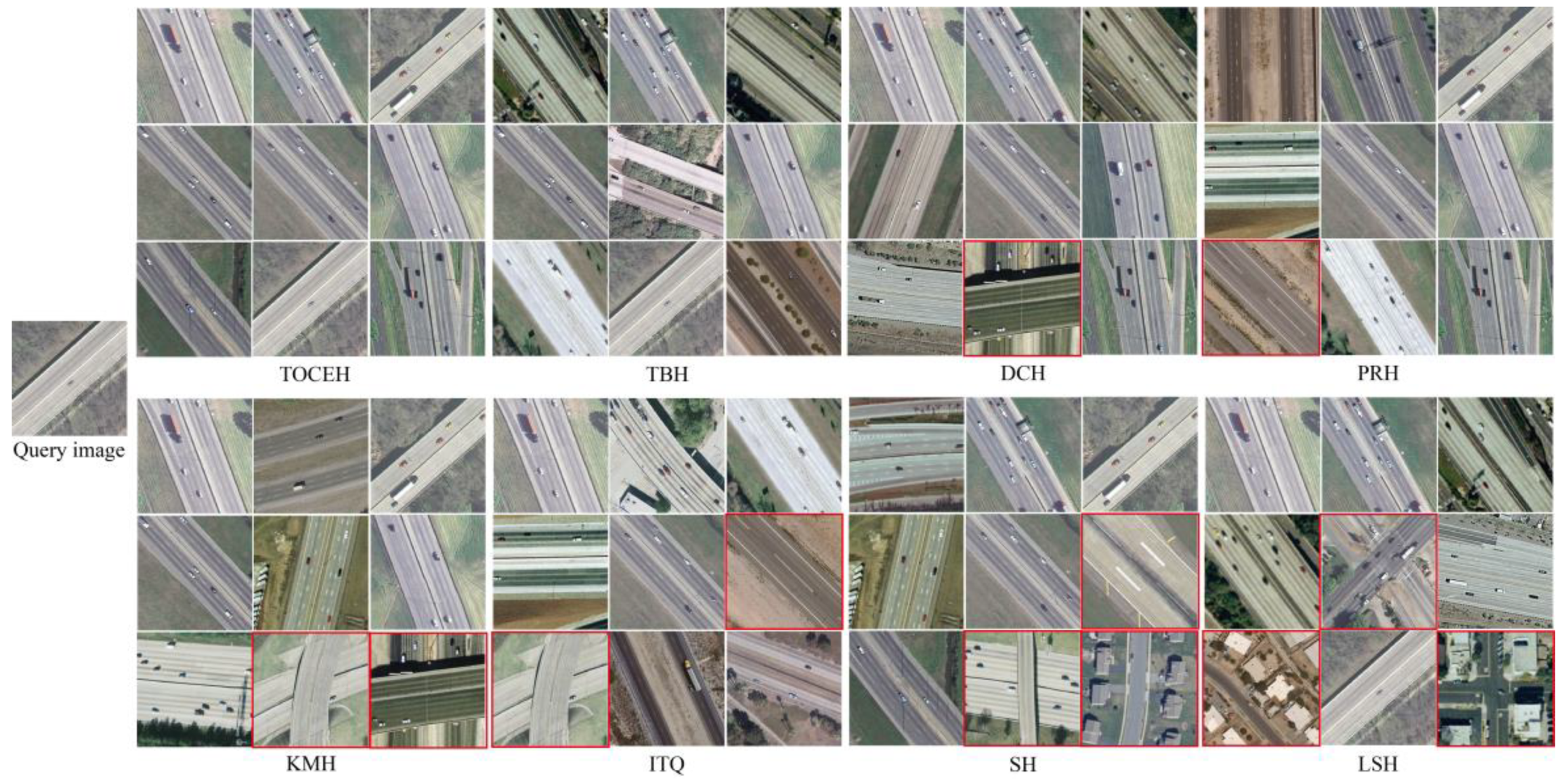
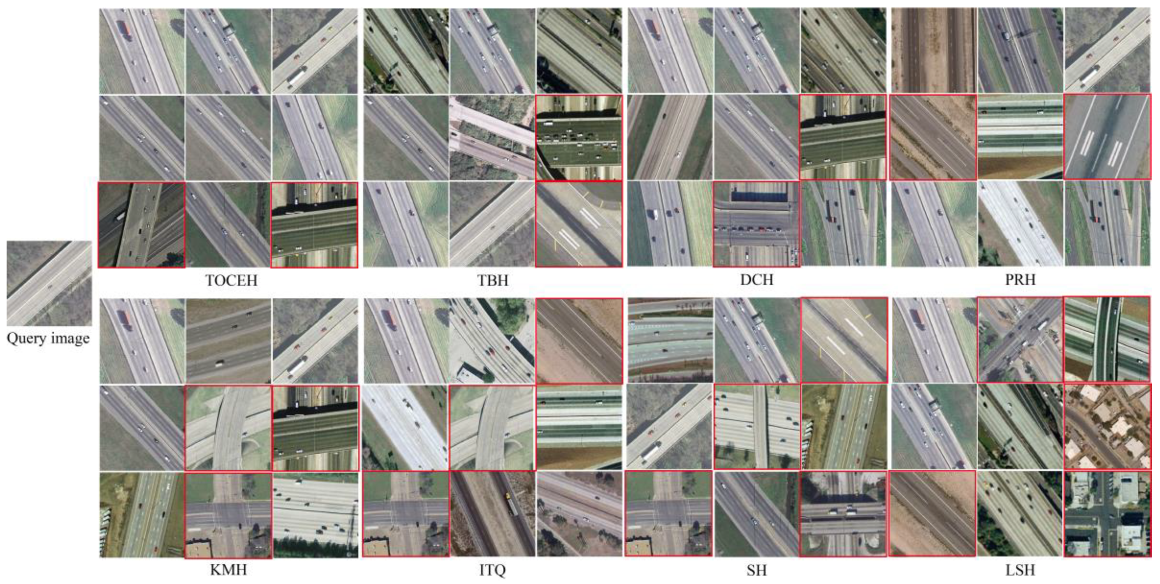
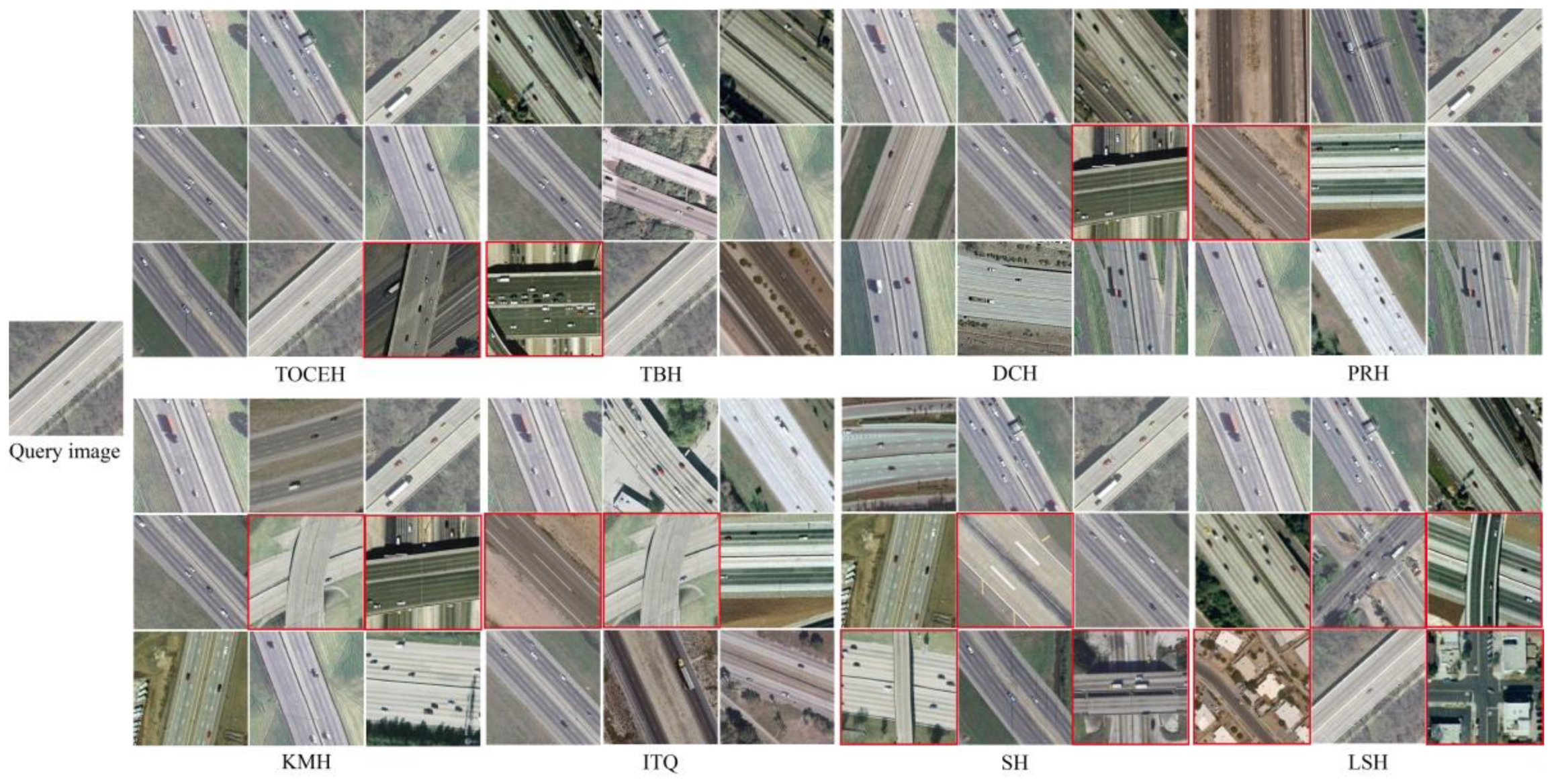
3.3.1. Qualitative Analysis

In this section, we show the qualitative image search results on the UCMD dataset [37]. The proposed TOCEH and the other seven state-of-the-art methods separately map the image content information into 64-, 128- and 256-bit binary code. The images with minimal Hamming distance to the query sample are returned as retrieval results and the false images are marked with red rectangles, as shown in Figure 7, Figure 8 and Figure 9.
From the RS image retrieval results, we intuitively know that TOCEH owns the best retrieval results. When encoding RS image content as a 64-bit binary code in Figure 6, TOCEH and TBH [10] return two false positive images. Correspondingly, the number of false images retrieved by the other six methods is larger than two. Furthermore, the false RS images’ ranking position in TOCEH is higher than that in TBH [10], which gives TOCEH a larger mAP value. In Figure 7, the length of the binary code is 128. One RS image is incorrectly returned by TOCEH, TBH [10], DCH [11] and PRH [23], and the false image has a relatively higher ranking position in TOCEH. As the number of binary bits increases to 256, only TOCEH and TBH [10] retrieve no false image, as shown in Figure 8.

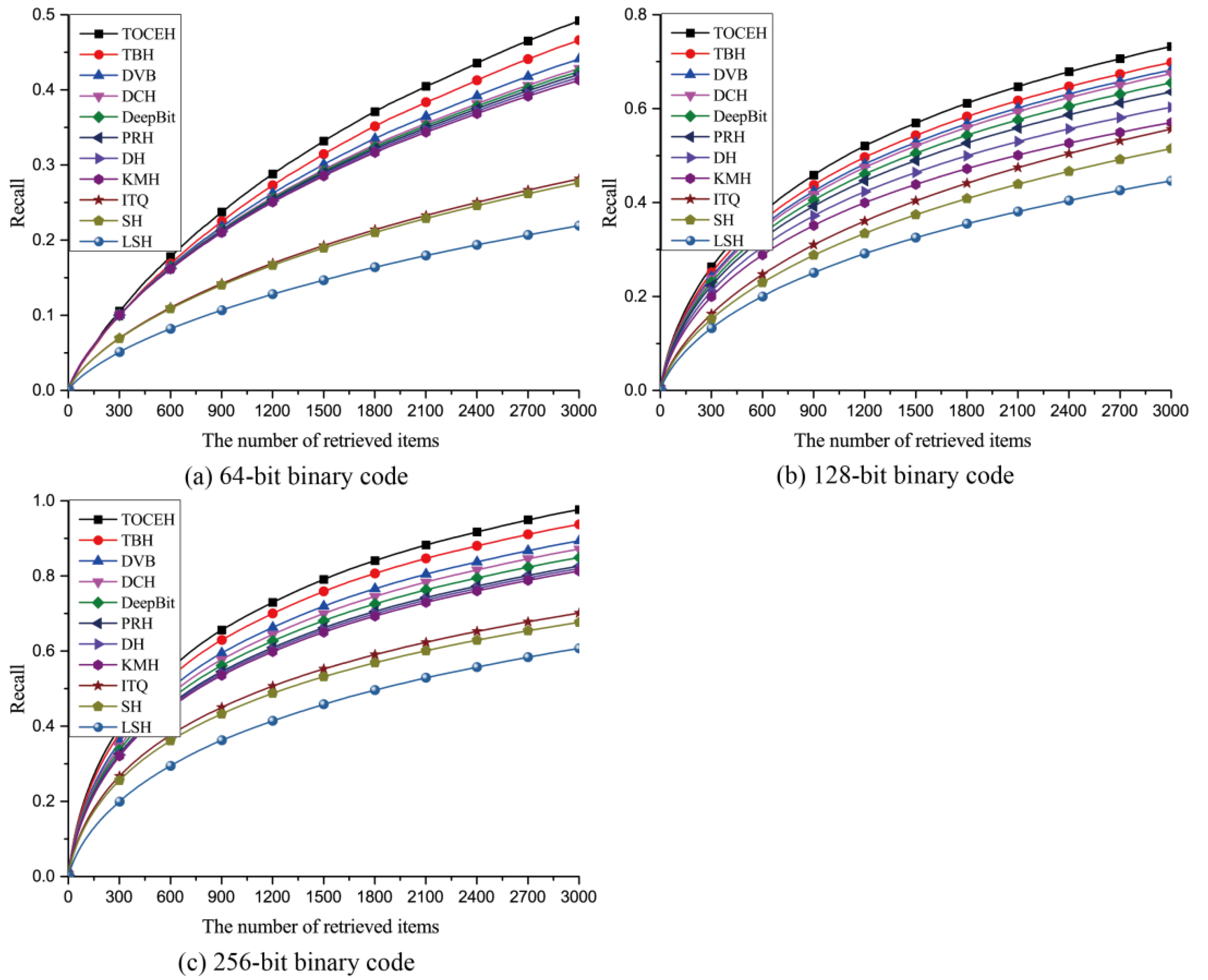
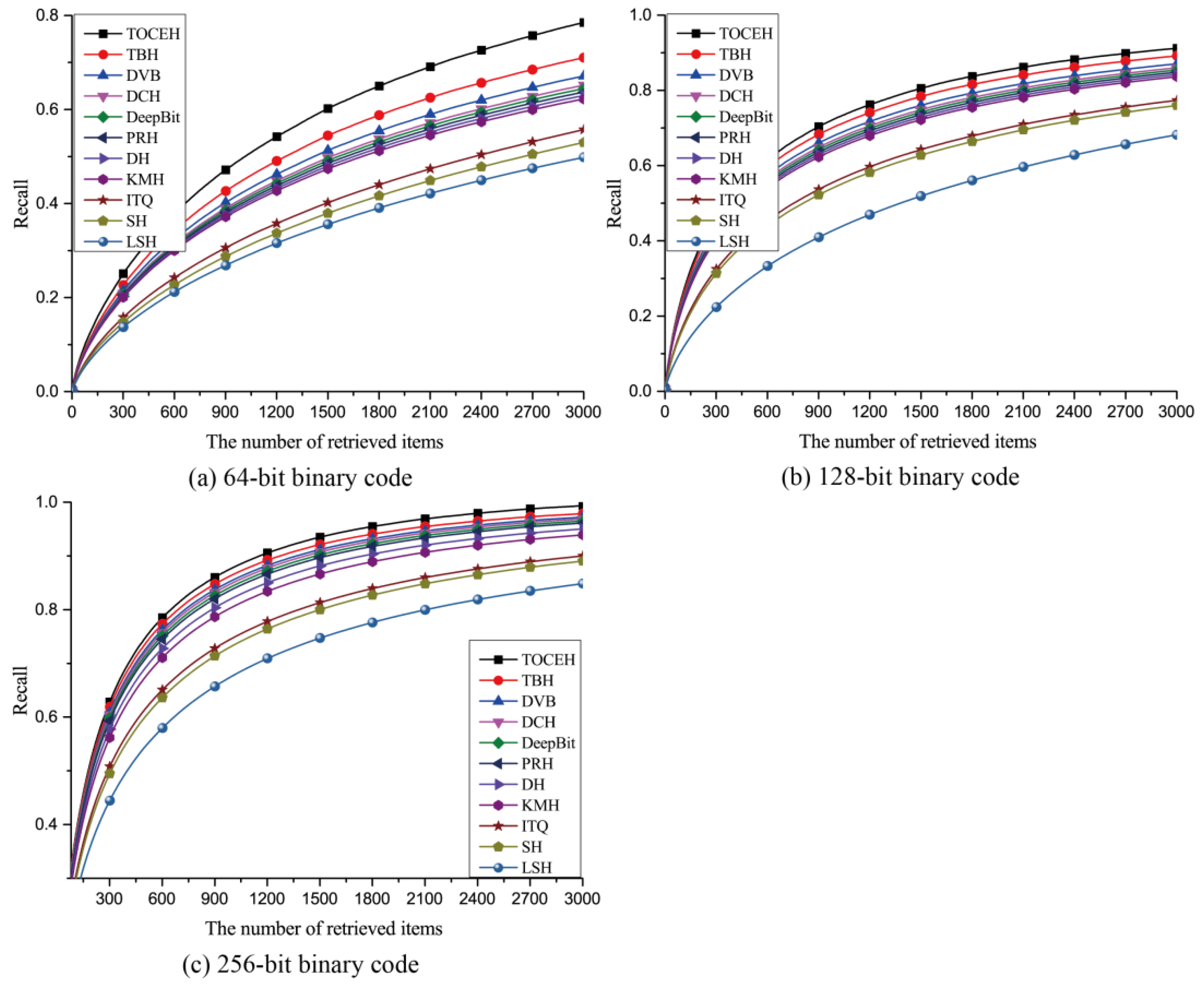
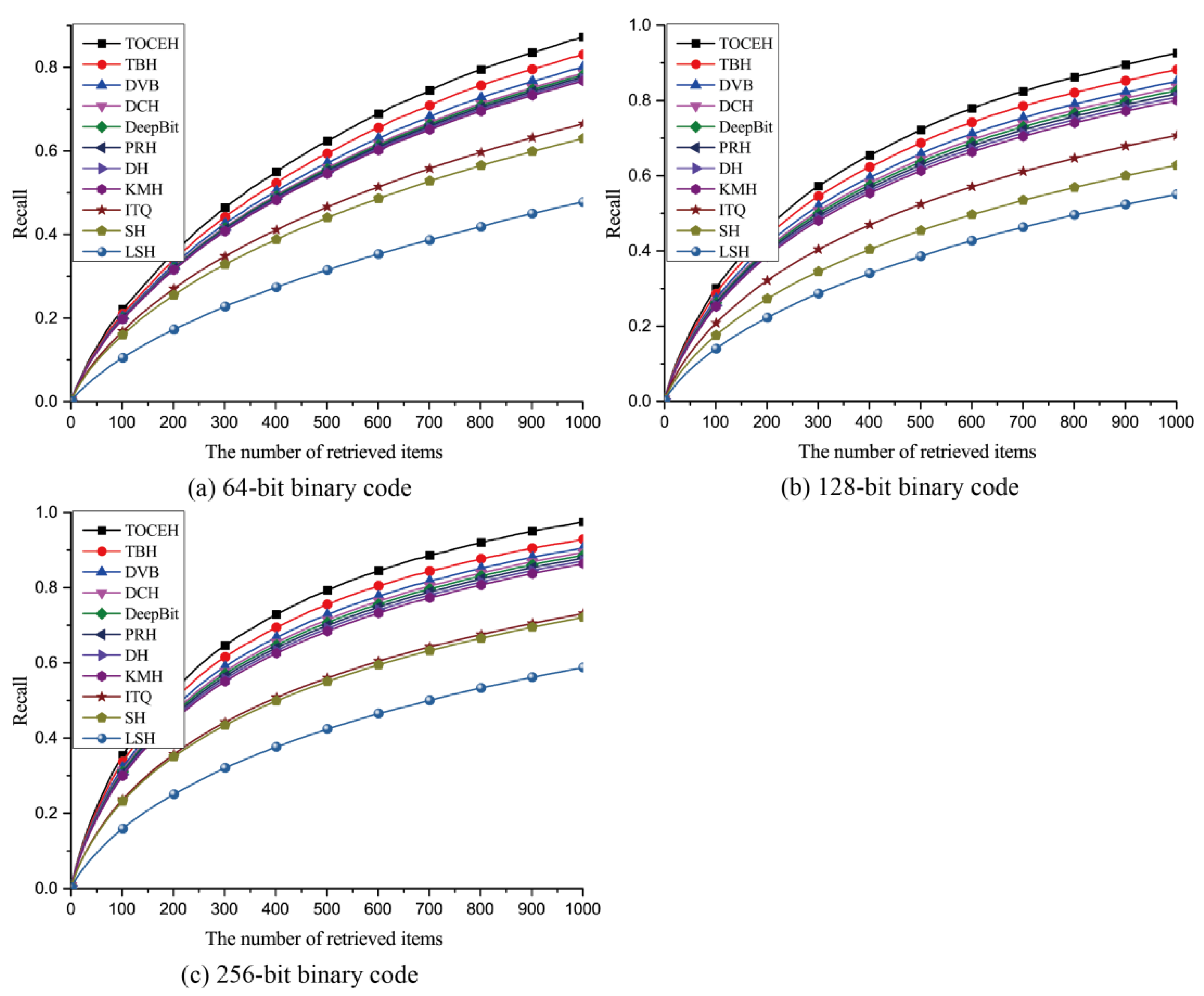
3.3.2. Quantitative Analysis

In this section, we adopt recall curves and mAP to quantitatively analyze the ANN search performance of the proposed TOCEH and the other seven state-of-the-art hashing methods. These hashing methods separately generate 64-, 128-, and 256-bit binary code to represent the image content. The mAP values are in Table 3, Table 4 and Table 5. The recall curves are shown in Figure 10, Figure 11 and Figure 12.
From the quantitative results, we know TOCEH achieves the best ANN search performance. LSH [14], the data-independent hashing algorithm, randomly generates hashing projection functions without a training process. As a result, the ANN search performance of LSH cannot drastically improve as the number of binary bits increases [9]. In contrast, the proposed TOCEH and the other nine comparative hashing methods utilize a machine learning mechanism to obtain the hashing functions, which are adaptive to the training data distribution. Thus, these machine-learning-based hashing algorithms achieve a better ANN search performance than LSH. SH [17] establishes a spectral graph to measure the similarity relation among samples, and divides the samples into different cluster groups by spectral graph partition. Then, SH [17] assigns the same code to the samples in the same group. For a large-scale RS image dataset, the time complexity of establishing a spectral graph would be high. Both ITQ [13] and KMH [12] first learn encoding centers, then assign the samples as the same binary code as their nearest center. ITQ [13] considers the fixed vertexes of a hyper cubic as centers, but they are not well adapted to the training data distribution. KMH [12] learns the encoding centers with minimal quantization loss and similarity loss by a k-means iterative mechanism. This measure effectively helps KMH improve the ANN search performance. To balance the training complexity and ANN search performance, PRH [23] employs the partial randomness and partial learning strategy to generate hashing functions. LSH [14], SH [17], ITQ [13], KMH [12] and PRH [23] belong to the shallow hashing algorithms, and their performances relate to the quality of the intermediate high dimensional features. To eliminate this effect, TOCEH, TBH [10], DVB [39], DH [40], DeepBit [41] and DCH [11] adopt a deep learning framework to learn the end-to-end binary feature, which can further boost the ANN search performance. The classical DH [40] proposes three constraints at the top layer of the deep network: the quantization loss, balance bits and independent bits. However, the pair-wise similarity preserving or the triplet ordinal relation preserving is not considered in DH. This may lead a poor performance of DH. The same problem also exists in DeepBit [41]. However, DeepBit augments the training data with different rotations and further updates the parameters of the network. This measure helps DeepBit to obtain a better ANN search performance than DH. For most deep hashing, it is hard to unveil the intrinsic structure of the whole sample space by simply regularizing the output codes within each single training batch. In contrast, the conditional auto-encoding variational Bayesian networks are introduced in DVB to exploit the feature space structure of the training data using the latent variables. DCH [11] pre-trains a similarity graph and expects that the probability distribution in the Hamming space should be consistent with that in the Euclidean space. TBH [10] abandons the process of the pre-computing similarity graph and embeds it in the deep neural network. TBH aims to preserve the similarity between the original data and the data decoded from the binary feature. Both TBH [10] and DCH [11] aim to preserve the pair-wise similarity, and it is difficult to capture the hyper structure among RS images. TOCEH establishes a tensor graph representing the triplet ordinal relation among RS images in both Hamming space and Euclidean space. During the training process, TOCEH expects that the triplet ordinal relation graphs have the same distribution in different spaces. Thus, it can enhance the ability of preserving the Euclidean ranking orders in the Hamming space. As discussed above, TOCEH can achieve the best RS image retrieval results.

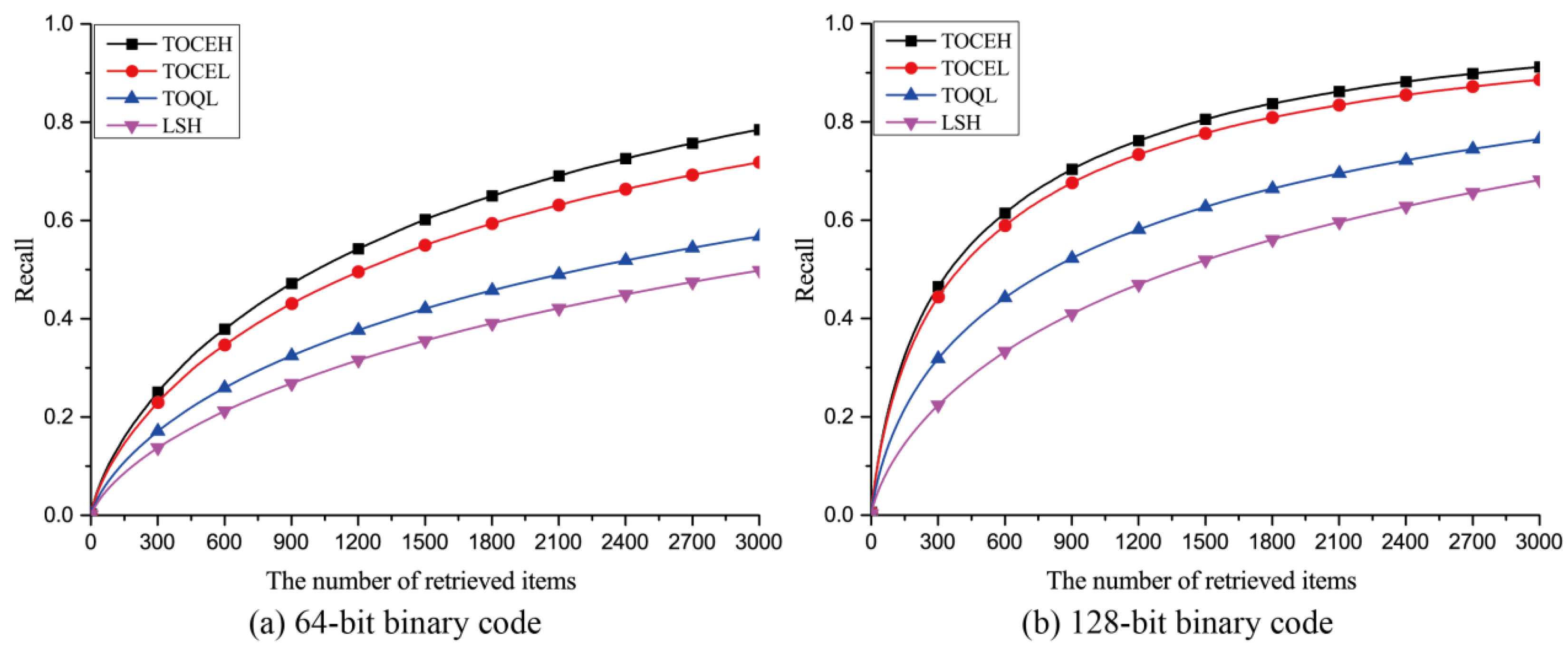
3.3.3. Ablation Experiments

To guarantee the ANN search performance of the obtained binary codes, the TOCEH algorithm proposes two key components: the triplet ordinal cross entropy loss and the triplet ordinal quantization loss. Here, we conduct the comparative experiments to analyze these two components. TOCEL only utilizes the triplet ordinal cross entropy loss as the objective function for deep learning binary code. The deep hashing TOQL only employs the triplet ordinal quantization loss as the objective function. TOCEH, TOCEL and TOQL separately map the data into 64- and 128-bit binary code. The ANN search results are shown in Figure 13, Figure 14 and Figure 15.
From the comparative results, we know that both the triplet ordinal cross entropy loss and the triplet ordinal quantization loss play important roles in improving the performance of TOCEH. The triplet ordinal cross entropy loss minimizes the inconsistency between the probability distributions of the triplet ordinal relations in different spaces. For example, the data pair (xi, xj) is more similar than data pair (xj, xk) in the Euclidean space. Then, to minimize the triplet ordinal cross entropy loss, it should be a larger probability to assign xi and xj as similar binary codes. Without the triplet ordinal cross entropy loss, TOQL randomly generates the samples’ binary codes. LSH algorithm also randomly generates the hashing functions. Thus, the ANN search performance of TOQL is almost the same as that of LSH. To fix the NP hard problem of the objective function, we apply the continuous relaxation mechanism to the binary encoding procedure. Furthermore, we define the triplet ordinal quantization loss to minimize the loss between the binary codes and the corresponding continuous variable. Without the triplet ordinal quantization loss, the difference between the optimized variables and the binary encoding results would become larger in TOCEL. Thus, TOCEL has a relatively inferior ANN search performance. As discussed above, both the triplet ordinal cross entropy loss and the triplet ordinal quantization loss are necessary for the TOCEH algorithm.

4. Conclusions

In this paper, to boost the RS image search performance in the Hamming space, we propose a novel deep hashing method called triplet ordinal cross entropy hashing (TOCEH) to learn an end-to-end binary feature of an RS image. Generally, most of the existing hashing methods place emphasis on preserving point-wise or pair-wise similarity. In contrast, TOCEH establishes a tensor graph to capture the triplet ordinal relation among RS images and defines the triplet ordinal relation preserving problem as the formulation of minimizing the cross entropy value. Then, TOCEH achieves the aim of preserving triplet ordinal relation by minimizing the inconsistency between the probability distributions of the triplet ordinal relations in different spaces. During the training process, to avoid the NP hard problem, we apply continuous relaxation to the binary encoding process. Furthermore, we define a quantization function based on the triplet ordinal relation preserving restriction, which can reduce the loss caused by the continuous procedure. Finally, the extensive comparative experiments conducted on three large-scale RS image datasets, including UCMD, SAT-4 and SAT-6, show that the proposed TOCEH outperforms many state-of-the-art hashing methods in RS image search tasks.

Author Contributions

Conceptualization, Z.W. and P.L.; methodology, Z.W. and N.W.; software, P.L. and X.Y.; validation, N.W., X.Y. and B.Y.; formal analysis, Z.W. and N.W.; investigation, P.L. and X.Y.; resources, B.Y.; data curation, B.Y.; writing—original draft preparation, Z.W.; writing—review and editing, P.L.; visualization, N.W. and X.Y.; supervision, Z.W. and P.L.; project administration, Z.W. and P.L.; funding acquisition, Z.W. All authors have read and agreed to the published version of the manuscript.

Funding

This research was funded by the National Natural Science Foundation of China, grant number 61841602, the Natural Science Foundation of Shandong Province of China, grant number ZR2018PF005, and the Fundamental Research Funds for the Central Universities, JLU, grant number 93K172021K12.

Acknowledgments

The authors express their gratitude to the institutions that supported this research: Shandong University of Technology (SDUT) and Jilin University (JLU).

Conflicts of Interest

The authors declare no conflict of interest.

References

  1. Cheng, Q.; Gan, D.; Fu, P.; Huang, H.; Zhou, Y. A Novel Ensemble Architecture of Residual Attention-Based Deep Metric Learning for Remote Sensing Image Retrieval. Remote Sens. 2021, 13, 3445. [Google Scholar] [CrossRef]
  2. Shan, X.; Liu, P.; Wang, Y.; Zhou, Q.; Wang, Z. Deep Hashing Using Proxy Loss on Remote Sensing Image Retrieval. Remote Sens. 2021, 13, 2924. [Google Scholar] [CrossRef]
  3. Shan, X.; Liu, P.; Gou, G.; Zhou, Q.; Wang, Z. Deep Hash Remote Sensing Image Retrieval with Hard Probability Sampling. Remote Sens. 2020, 12, 2789. [Google Scholar] [CrossRef]
  4. Kong, J.; Sun, Q.; Mukherjee, M.; Lloret, J. Low-Rank Hypergraph Hashing for Large-Scale Remote Sensing Image Retrieval. Remote Sens. 2020, 12, 1164. [Google Scholar] [CrossRef] [Green Version]
  5. Han, L.; Li, P.; Bai, X.; Grecos, C.; Zhang, X.; Ren, P. Cohesion Intensive Deep Hashing for Remote Sensing Image Retrieval. Remote Sens. 2020, 12, 101. [Google Scholar] [CrossRef] [Green Version]
  6. Hou, Y.; Wang, Q. Research and Improvement of Content Based Image Retrieval Framework. Int. J. Pattern. Recogn. 2018, 32, 1850043.1–1850043.14. [Google Scholar] [CrossRef]
  7. Liu, Y.; Zhang, D.; Lu, G.; Ma, W.Y. A survey of content-based image retrieval with high-level semantics. Pattern. Recogn. 2007, 40, 262–282. [Google Scholar] [CrossRef]
  8. Wang, J.; Zhang, T.; Song, J.; Sebe, N.; Shen, H.T. A Survey on Learning to Hash. IEEE Trans. Pattern. Anal. 2018, 40, 769–790. [Google Scholar] [CrossRef]
  9. Wang, J.; Liu, W.; Kumar, S.; Chang, S.F. Learning to Hash for Indexing Big Data—A Survey. Proc. IEEE 2016, 104, 34–57. [Google Scholar] [CrossRef]
  10. Shen, Y.; Qin, J.; Chen, J.; Yu, M.; Liu, L.; Zhu, F.; Shen, F.; Shao, L. Auto-encoding twin-bottleneck hashing. In Proceedings of the Conference on Computer Vision and Pattern Recognition, Seattle, WA, USA, 13–19 June 2020; pp. 2815–2824. [Google Scholar]
  11. Cao, Y.; Long, M.; Liu, B.; Wang, J. Deep cauchy hashing for hamming space retrieval. In Proceedings of the Conference on Computer Vision and Pattern Recognition, Salt Lake City, UT, USA, 18–23 June 2018; pp. 1229–1237. [Google Scholar]
  12. He, K.; Wen, F.; Sun, J. K-means hashing: An affinity-preserving quantization method for learning binary compact codes. In Proceedings of the Conference on Computer Vision and Pattern Recognition, Portland, OR, USA, 23–28 June 2013; pp. 2938–2945. [Google Scholar]
  13. Gong, Y.; Lazebnik, S.; Gordo, A.; Perronnin, F. Iterative Quantization: A Procrustean Approach to Learning Binary Codes for Large-Scale Image Retrieval. IEEE Trans. Pattern. Anal. 2013, 35, 2916–2929. [Google Scholar] [CrossRef] [Green Version]
  14. Datar, M.; Immorlica, N.; Indyk, P.; Mirrokni, V.S. Locality-sensitive hashing scheme based on p-stable distributions. In Proceedings of the 20th ACM Symposium on Computational Geometry, Brooklyn, NY, USA, 8–11 June 2004; pp. 253–262. [Google Scholar]
  15. Cao, Y.; Liu, B.; Long, M.; Wang, J. HashGAN: Deep learning to hash with pair conditional Wasserstein GAN. In Proceedings of the Conference on Computer Vision and Pattern Recognition, Salt Lake City, UT, USA, 18–23 June 2018; pp. 1287–1296. [Google Scholar]
  16. Liu, H.; Wang, R.; Shan, S.; Chen, X. Deep supervised hashing for fast image retrieval. In Proceedings of the Conference on Computer Vision and Pattern Recognition, Las Vegas, NV, USA, 27–30 June 2016; pp. 2064–2072. [Google Scholar]
  17. Weiss, Y.; Torralba, A.; Fergus, R. Spectral hashing. In Proceedings of the Advances in Neural Information Processing Systems, Vancouver, BC, Canada, 8–11 December 2008; pp. 1753–1760. [Google Scholar]
  18. Lowe, D.G. Distinctive image features from scale-invariant keypoints. Int. J. Comput. Vis. 2004, 60, 91–110. [Google Scholar] [CrossRef]
  19. Oliva, A.; Torralba, A. Modeling the shape of the scene: A holistic representation of the spatial envelope. Int. J. Comput. Vis. 2001, 42, 145–175. [Google Scholar] [CrossRef]
  20. Shen, F.; Xu, Y.; Liu, L.; Yang, Y.; Huang, Z.; Shen, H.T. Unsupervised Deep Hashing with Similarity-Adaptive and Discrete Optimization. IEEE Trans. Pattern. Anal. 2018, 40, 3034–3044. [Google Scholar] [CrossRef] [PubMed]
  21. Wang, Y.; Song, J.; Zhou, K.; Liu, Y. Unsupervised deep hashing with node representation for image retrieval. Pattern. Recogn. 2021, 112, 107785. [Google Scholar] [CrossRef]
  22. Zhang, M.; Zhe, X.; Chen, S.; Yan, H. Deep Center-Based Dual-Constrained Hashing for Discriminative Face Image Retrieval. Pattern. Recogn. 2021, 117, 107976. [Google Scholar] [CrossRef]
  23. Li, P.; Ren, P. Partial Randomness Hashing for Large-Scale Remote Sensing Image Retrieval. IEEE Geosci. Remote Sens. 2017, 14, 1–5. [Google Scholar] [CrossRef]
  24. Demir, B.; Bruzzone, L. Hashing-Based Scalable Remote Sensing Image Search and Retrieval in Large Archives. IEEE Trans. Geosci. Remote Sens. 2016, 54, 892–904. [Google Scholar] [CrossRef]
  25. Li, Y.; Zhang, Y.; Huang, X.; Zhu, H.; Ma, J. Large-Scale Remote Sensing Image Retrieval by Deep Hashing Neural Networks. IEEE Trans. Geosci. Remote Sens. 2017, 56, 950–965. [Google Scholar] [CrossRef]
  26. Fan, L.; Zhao, H.; Zhao, H. Distribution Consistency Loss for Large-Scale Remote Sensing Image Retrieval. Remote Sens. 2020, 12, 175. [Google Scholar] [CrossRef] [Green Version]
  27. Krizhevsky, A.; Sutskever, I.; Hinton, G.E. ImageNet classification with deep convolutional neural networks. In Proceedings of the NIPS, Lake Tahoe, NV, USA, 3–6 December 2012; pp. 1106–1114. [Google Scholar]
  28. Russakovsky, O.; Deng, J.; Su, H.; Krause, J.; Satheesh, S.; Ma, S.; Huang, Z.; Karpathy, A.; Khosla, A.; Bernstein, M.S.; et al. ImageNet Large Scale Visual Recognition Challenge. Int. J. Comput. Vis. 2015, 115, 211–252. [Google Scholar] [CrossRef] [Green Version]
  29. Wang, Z.; Sun, F.Z.; Zhang, L.B.; Wang, L.; Liu, P. Top Position Sensitive Ordinal Relation Preserving Bitwise Weight for Image Retrieval. Algorithms 2020, 13, 18. [Google Scholar] [CrossRef] [Green Version]
  30. Liu, H.; Ji, R.; Wang, J.; Shen, C. Ordinal Constraint Binary Coding for Approximate Nearest Neighbor Search. IEEE Trans. Pattern Anal. 2019, 41, 941–955. [Google Scholar] [CrossRef] [PubMed]
  31. Liu, H.; Ji, R.; Wu, Y.; Liu, W. Towards optimal binary code learning via ordinal embedding. In Proceedings of the 30th AAAI Conference on Artificial Intelligence, Phoenix, AZ, USA, 12–17 February 2016; pp. 1258–1265. [Google Scholar]
  32. Wang, J.; Liu, W.; Sun, A.X.; Jiang, Y.G. Learning hash codes with listwise supervision. In Proceedings of the IEEE International Conference on Computer Vision, Sydney, NSW, Australia, 1–8 December 2013; pp. 3032–3039. [Google Scholar]
  33. Norouzi, M.; Fleet, D.J.; Salakhutdinov, R. Hamming distance metric learning. In Proceedings of the Advances in Neural Information Processing Systems, Lake Tahoe, NV, USA, 3–6 December 2012; pp. 1061–1069. [Google Scholar]
  34. Wang, Q.; Zhang, Z.; Luo, S. Ranking preserving hashing for fast similarity search. In Proceedings of the International Conference on Artificial Intelligence, Buenos Aires, Argentina, 25–31 July 2015; pp. 3911–3917. [Google Scholar]
  35. Liu, L.; Shao, L.; Shen, F.; Yu, M. Discretely coding semantic rank orders for supervised image hashing. In Proceedings of the Computer Vision and Pattern Recognition, Honolulu, HI, USA, 21–26 July 2017; pp. 5140–5149. [Google Scholar]
  36. Chen, S.; Shen, F.; Yang, Y.; Xu, X.; Song, J. Supervised hashing with adaptive discrete optimization for multimedia retrieval. Neurocomputing 2017, 253, 97–103. [Google Scholar] [CrossRef]
  37. Yang, Y.; Newsam, S.D. Bag-of-visual-words and spatial extensions for land-use classification. In Proceedings of the 18th SIGSPATIAL International Conference on Advances in Geographic Information Systems, San Jose, CA, USA, 3–5 November 2010; pp. 270–279. [Google Scholar]
  38. Basu, S.; Ganguly, S.; Mukhopadhyay, S.; DiBiano, R.; Karki, M.; Nemani, R.R. DeepSat: A learning framework for satellite imagery. In Proceedings of the 23rd SIGSPATIAL International Conference on Advances in Geographic Information Systems, Bellevue, WA, USA, 3–6 November 2015; pp. 1–10. [Google Scholar]
  39. Shen, Y.; Liu, L.; Shao, L. Unsupervised Binary Representation Learning with Deep Variational Networks. Int. J. Comput. Vis. 2019, 127, 1614–1628. [Google Scholar] [CrossRef]
  40. Liong, V.E.; Lu, J.; Wang, G.; Moulin, P.; Zhou, J. Deep hashing for compact binary codes learning. In Proceedings of the Conference on Computer Vision and Pattern Recognition, Boston, MA, USA, 7–12 June 2015; pp. 1063–6919. [Google Scholar]
  41. Lin, K.; Lu, J.; Chen, C.S.; Zhou, J. Learning compact binary descriptors with unsupervised deep neural networks. In Proceedings of the Conference on Computer Vision and Pattern Recognition (CVPR), Las Vegas, NV, USA, 27–30 June 2016; pp. 1063–6919. [Google Scholar]
Figure 1. Flowchart of the proposed TOCEH algorithm. Firstly, to represent the image content, we use the Alexnet, including five convolutional (CONV) networks and two fully connected (FC) networks, to learn the continuous latent variable. Secondly, the triplet ordinal relation is computed by the tensor product of the similarity and dissimilarity graphs. Thirdly, two fully connected layers with the activation function of ReLU are utilized to generate the binary code. To guarantee the performance, we define the triplet ordinal cross entropy loss to minimize the inconsistency between the triplet ordinal relations in different spaces. Furthermore, we design the triplet ordinal quantization loss to reduce the loss caused by the relaxation mechanism.
Remotesensing 13 04786 g001
Figure 2. The marked elements are picked up to restore in a matrix with the size of N × N × N.
Remotesensing 13 04786 g002
Figure 3. The characteristic of the function (∙).
Remotesensing 13 04786 g003
Figure 4. Sample images of the UCMD dataset.
Remotesensing 13 04786 g004
Figure 5. Sample images of the SAT-4 dataset.
Remotesensing 13 04786 g005
Figure 6. Sample images of the SAT-6 dataset.
Remotesensing 13 04786 g006
Figure 7. The RS image retrieval results on the UCMD dataset, and the length of the binary code is 64. The false images are marked with red rectangles.
Remotesensing 13 04786 g007
Figure 8. The RS image retrieval results on the UCMD dataset, and the length of the binary code is 128. The false images are marked with red rectangles.
Remotesensing 13 04786 g008
Figure 9. The RS image retrieval results on the UCMD dataset, and the length of the binary code is 256. The false images are marked with red rectangles.
Remotesensing 13 04786 g009
Figure 10. The recall curves of all comparative methods on UCMD; the data are separately encoded as (a) 64-, (b) 128- and (c) 256-bit binary code.
Remotesensing 13 04786 g010
Figure 11. The recall curves of all comparative methods on SAT-4 and the data are separately encoded as (a) 64-, (b) 128- and (c) 256-bit binary code.
Remotesensing 13 04786 g011
Figure 12. The recall curves of all comparative methods on SAT-6 and the data are separately encoded as (a) 64-, (b) 128- and (c) 256-bit binary code.
Remotesensing 13 04786 g012
Figure 13. The ablation experiments on UCMD. The data are separately encoded as (a) 64- and (b) 128-bit binary code.
Remotesensing 13 04786 g013
Figure 14. The ablation experiments on SAT-4. The data are separately encoded as (a) 64- and (b) 128-bit binary code.
Remotesensing 13 04786 g014
Figure 15. The ablation experiments on SAT-6. The data are separately encoded as (a) 64- and (b) 128-bit binary code.
Remotesensing 13 04786 g015
Table 1. The important notations used in this paper.
NotationDescription
BCompact binary code matrix
Bi, Bj, BkThe i-th, j-th, k-th column in B
H(∙)Hashing function
XData matrix in the Euclidean space
xi, xj, xkThe i-th, j-th, k-th column in X
GTriplet ordinal graph in the Euclidean space
ĜTriplet ordinal relation in the Hamming space
gijkThe entry (i, j, k) in G
SSimilarity graph
DSDissimilarity graph
NThe number of training samples
LThe number of k-means centers
P(∙)Probability distribution function
dh(∙,∙)Hamming distance function
MBinary code length
1The binary matrix with all values of 1
Table 2. Statistics and several parameter settings of three datasets.
UCMDSAT4SAT6
Class Number2146
Image Size256 × 25628 × 2828 × 28
Dataset Size2100500,000405,000
Training Set1470400,000360,000
Query Set630100,00045,000
Ground Truth10010001000
Table 3. Comparison of mAP with different binary code lengths on UCMD.
TOCEHTBHDVBDCHDeepBitPRHDHKMHITQSHLSH
64-bit0.39140.34150.32610.29170.26570.24620.22960.21350.19860.17240.1637
128-bit0.54790.46380.42590.39630.37810.35270.34670.28160.24620.20150.1842
256-bit0.58370.49750.47570.43190.41970.37460.35280.31680.26730.23510.2148
Table 4. Comparison of mAP with different binary code lengths on SAT-4.
TOCEHTBHDVBDCHDeepBitPRHPRHKMHITQSHLSH
64-bit0.70110.57680.52710.48620.45220.43610.41390.39460.36570.34820.3407
128-bit0.72360.61240.55370.49860.47940.45280.43850.41730.38560.37240.3615
256-bit0.75280.63450.61490.51280.50680.48570.46530.43610.42850.41520.3986
Table 5. Comparison of mAP with different binary code lengths on SAT-6.
TOCEHTBHDVBDCHDeepBitPRHDHKMHITQSHLSH
64-bit0.71240.58260.54460.49360.47250.45860.43520.41250.37640.36950.3628
128-bit0.73510.62680.58410.51740.49210.47950.45960.42810.39270.38640.3752
256-bit0.78420.65270.62610.53940.51750.49720.46280.45160.43590.42380.4175
Publisher’s Note: MDPI stays neutral with regard to jurisdictional claims in published maps and institutional affiliations.

