Soil Organic Carbon Content Prediction Using Soil-Reflected Spectra: A Comparison of Two Regression Methods

Abstract

Quantifying the organic carbon content of soil over large areas is essential for characterising the soil and the effects of its management. However, analytical methods can be laborious and costly. Reflectance spectroscopy is a well-established and widespread method for estimating the chemical-element content of soils. The aim of this study was to estimate the soil organic carbon (SOC) content using hyperspectral remote sensing. The data were from soils from two localities in the semi-arid region of Brazil. The spectral reflectance factors of the collected soil samples were recorded at wavelengths ranging from 350–2500 nm. Pre-processing techniques were employed, including normalisation, Savitzky–Golay smoothing and first-order derivative analysis. The data (n = 65) were examined both jointly and by soil class, and subdivided into calibration and validation to independently assess the performance of the linear methods. Two multivariate models were calibrated using the SOC content estimated in the laboratory by principal component regression (PCR) and partial least squares regression (PLSR). The study showed significant success in predicting the SOC with transformed and untransformed data, yielding acceptable-to-excellent predictions (with the performance-to-deviation ratio ranging from 1.40–3.38). In general, the spectral reflectance factors of the soils decreased with the increasing levels of SOC. PLSR was considered more robust than PCR, whose wavelengths from 354 to 380 nm, 1685, 1718, 1757, 1840, 1876, 1880, 2018, 2037, 2042, and 2057 nm showed outstanding absorption characteristics between the predicted models. The results found here are of significant practical value for estimating SOC in Neosols and Cambisols in the semi-arid region of Brazil using VIS-NIR-SWIR spectroscopy.

1. Introduction

From a synoptic perspective, soil quality assessment includes the integration of physical, biological, and chemical properties as quality indicators [1]. However, as these key properties vary dynamically over space and time, such assessments represent a stimulating task for the academic community.

Soil Organic Carbon (SOC) is recognised by farmers and scientists as a primary indicator of soil quality. Representing around 58% of the structure of organic matter (OM), SOC is considered the main carbon stock at the terrestrial level [2,3], with estimates of up to three times more C than are contained in the atmosphere [4]. In light of this view, the assumption remains that increases in SOC content are the result of a greater input of organic matter to the medium [5]. Arguably, soil fertility is favoured by a higher concentration of OM, a result of the storage and release of nutrients [6]; stabilisation of the physical structure [7]; improvement in water retention capacity, biodiversity of the soil and contaminant biodegradation [8]; and the aggregation and sorption of organic and inorganic pollutants [9], among other benefits.

Quantitative assessments of SOC and its management are needed to understand its key role in the global C cycle [10]. However, conventional SOC quantification can be laborious and expensive, and it is capable of producing significant amounts of non-recyclable waste. Added to this is the need for a high number of samples to maintain the statistical robustness of the analysis. Determined by the conversion into CO₂ of organic components found in a sample, dry combustion [11] uses a muffle furnace or automated elemental analyser [12] for burning and then determining organic matter by means of the van Bemmelen correction factor. Despite demonstrating better precision in quantifying SOC and employing certified high-purity chemical reagents, this method incurs high maintenance and analysis costs [13]. On the other hand, wet combustion [14,15] can be obtained by means of the digestion, oxidation, and titration of the remaining oxidising agent [16]. In contrast to the low cost of equipment and reagents [12], this type of estimation presents critical analytical and environmental problems, due to the production of toxic waste, such as potassium dichromate (K₂Cr₂O₇) and sulphuric acid (H₂SO₄) [17].

As an alternative to laboratory practices that demand more time for analysis and the use of substantially dangerous reagents [18], the technique of reflectance spectroscopy has become ever more prominent in evaluating SOC [19]. Using physical parameters such as reflectance factors (ρ) [20,21], hyperspectral remote sensing (HRS) has made it possible to detect soil constituents and predict soil properties indirectly by investigating the electromagnetic radiation reflected by the surface of a sample [22]. The principle of reflectance spectroscopy in soil science is related to changes in the surface of the material and in its optically active constituents [23,24], since SOC significantly affects the form and nature of soil reflectance spectra [25], and it can be estimated rapidly [10,19,26].

Thus, using a fast, economically competitive and non-destructive approach that produces no residue, HRS allows several properties of a sample to be evaluated from a single spectral reading. Visible and near-infrared (VIS-NIR) spectroscopy has gradually demonstrated its potential for estimating SOC [27], and is a powerful alternative to conventional chemical analysis [28,29,30].

Since they demonstrate high accuracy, in situ quantitative SOC estimates using a portable spectrometer are preferred to the conventional method, as they avoid transportation, drying, crushing, sieving or laboratory procedures [31]. Although the accuracy of in situ SOC predictions is generally more limited than those in the laboratory, researchers [32,33,34,35] report promising results for both types of spectral data using a combination of chemometric and multivariate techniques.

Allowing that hyperspectral sensors acquire an extensive amount of data concerning oscillations in the electromagnetic spectrum [36], various types of multivariate analysis are suitable for reducing the dimensionality of the input data [37]. This makes it possible to study only those wavelengths (λ) that best express the variance in the structure of the original data on soil properties [38,39]. It is in this context that Partial Least Squares Regression (PLSR) and Principal Components Regression (PCR) are recommended by several authors [40,41,42,43,44] when estimating soil attributes from hyperspectral data.

Statistical deviation metrics, such as the coefficient of determination (R²), the Root Mean Square Error (RMSE), and the Ratio of Prediction Deviation (RPD) are useful for evaluating performance in chemometric analysis. Comparing multivariate methods of estimating SOC, Morellos et al. [43] selected 140 samples of agricultural soil immediately after the wheat harvest, and achieved an R² of 0.711 and RPD of 1.86 for PLSR, and an R² of 0.724 and RPD of 1.89 with principal component regression (PCR). Analysing saline soils, Mahajan et al. [44] pointed out the slight superiority of the PLSR method, with an R² of 0.68, RMSE of 1.53 and RPD of 0.41, compared to the PCR method, which recorded an R² of 0.58, an RMSE of 1.67, and an RPD of 0.38, even when using 36 principal components.

This article, therefore, proposes a practical view of the relevance of multivariate techniques using hyperspectral data in the rapid quantification of the SOC stock of soils. As such, the aim was to estimate the SOC present in two classes of soil in a semi-arid region of Brazil based on their spectral information between 350–2500 nm. Among the main contributions of this study are: (i) the identification of wavelengths showing the best correlation with the SOC content in the soil samples; (ii) the identification of the best mathematical transformations of the spectral data for optimising the estimation using PLSR and PCR; and (iii) the construction of SOC linear estimation models for each spectral transformation under evaluation.

2. Materials and Methods

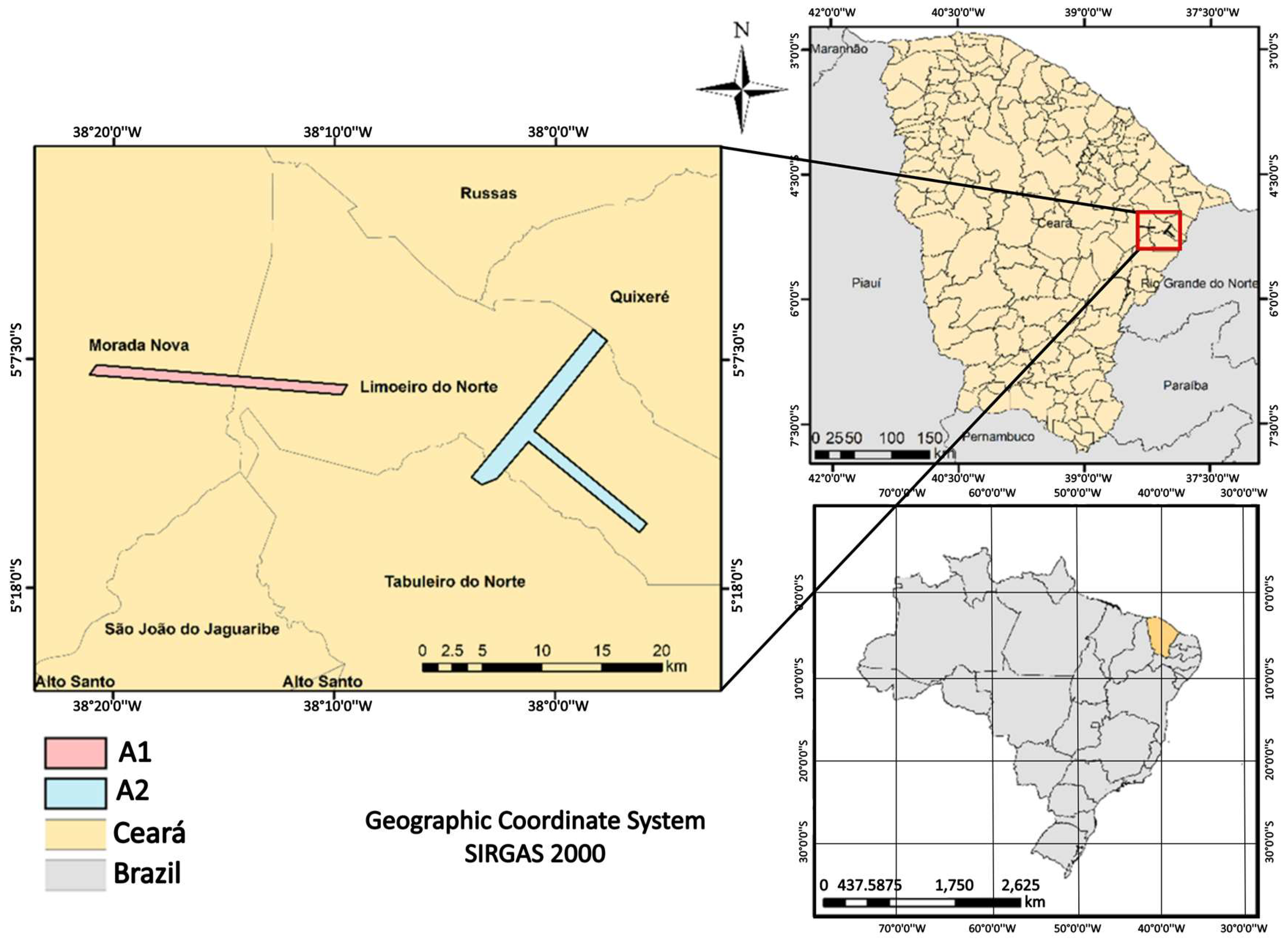
2.1. Description of the Study Areas

The present work studied the soils of two different areas of a semi-arid region of Brazil in the state of Ceará. Area 1 (A1) and Area 2 (A2) are described in

Table 1. Description of the sampling areas and analysed soils, as per the Brazilian System of Soil Classification (SiBCS), with the soil taxonomy in brackets.

Attribute	A1	A2
Municipality	Morada Nova, Ceará	Limoeiro do Norte, Ceará
Hydrographic basin	Banabuiú	Lower Jaguaribe
area	18.22 km2	37.65 km2
Predominant soil class	Fluvic Neosols (Fluvents)	Haplic Cambisols (Typic Dystrudept)
Predominant textural classes	Sandy-loam to Silt-clay-loam	Sandy-loam to Clay
Mean particle size (sand-silt-clay) [45]	44%-35%-21%	48%-22%-30%
Number of samples collected	29	36

based on their most distinct characteristics.

According to the Köppen classification, the predominant climate, both in the Irrigated Perimeter of Morada Nova (A1) and in Jagaribe-Apodi (A2), is considered type BS W’h’, which is characterised as very hot and semi-arid, with a mean temperature of 27.5 °C, a minimum of 26 °C and a maximum of 32 °C. The rainy season, with a mean rainfall of around 660 mm, usually starts in January and can last until June, with 80% of the rainfall concentrated in March, April, and May. Rainfall distribution in the region, however, is irregular, resulting in marked deviations around the mean [46].

Figure 1 shows the spatial distribution map of these soils in each of the study areas. The region comprising area A1 is characterised by the predominant occurrence of soils of the Fluvic Neosol class, poorly developed soils without a B horizon, resulting from the deposition of alluvial sediments that may make up part of the organic material present in the soil, as they are close to the floodplains of the main water courses in the region [47]. According to authors such as [48,49,50], these soils present a mineralogical mixture of expansive and non-expansive clays that predominate in relation to kaolinite. Cunha et al. [51] report that, as these soils have developed from recent alluvial sediments and have no pedogenetic relationship, they feature vertically or horizontally diversified granulometry, showing the heterogeneity of the source material.

According to Jacomine et al. [47], area A2 is characterised by the occurrence of Eutrophic Haplic Cambisols from limestone rocks, also poorly developed, with an incipient B horizon, and marked by the presence of high-activity clay and a high base saturation (≥50%). These, in turn, show more textural uniformity and may feature a loamy-sandy or more clayey texture, with a predominance of kaolinite as well as a significant presence of iron oxides (goethite and hematite) [51,52]. Another class of soil occurring in area A2, indicated by the above authors, albeit without much evidence, is Vertisols.

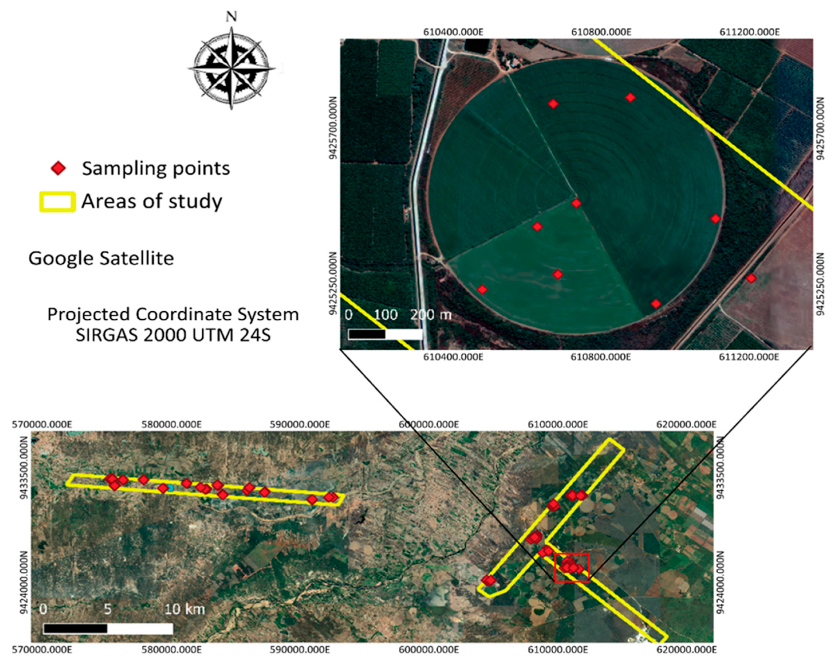
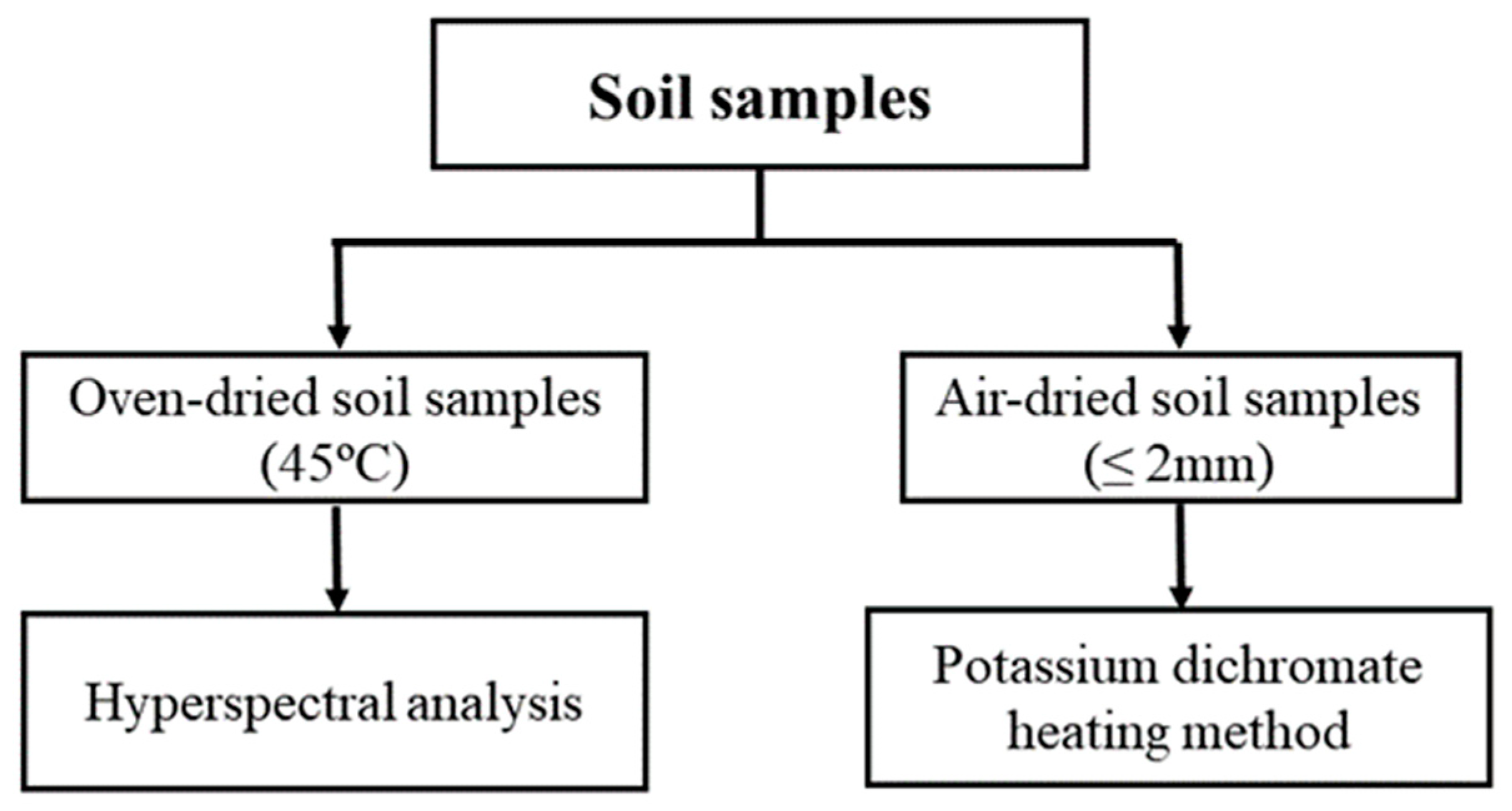
2.2. Collection of the Samples

Two subsets of disturbed samples were used, collected at depths of between 0.0 and 10.0 cm. Considering the close connection of texture with variations in the organic carbon content of the soil, spatial independence, and the significant short-distance variability of the clay minerals [53], the samples used were chosen based on two criteria: (i) the spatial distribution of the collection points; and (ii) the similarity of the clay content.

Cluster analysis was carried out to determine the textural similarity between the points sampled in each area, based on the clay content quantified [45] for each point. The pipette method described by Amaro Filho et al. [54] was used. The clusters formed by the most-similar samples were separated by a Euclidean distance of 0.07. Within each cluster, the spatial distance between the collection points was evaluated, and those most representative of the areas of interest were selected (Figure 2).

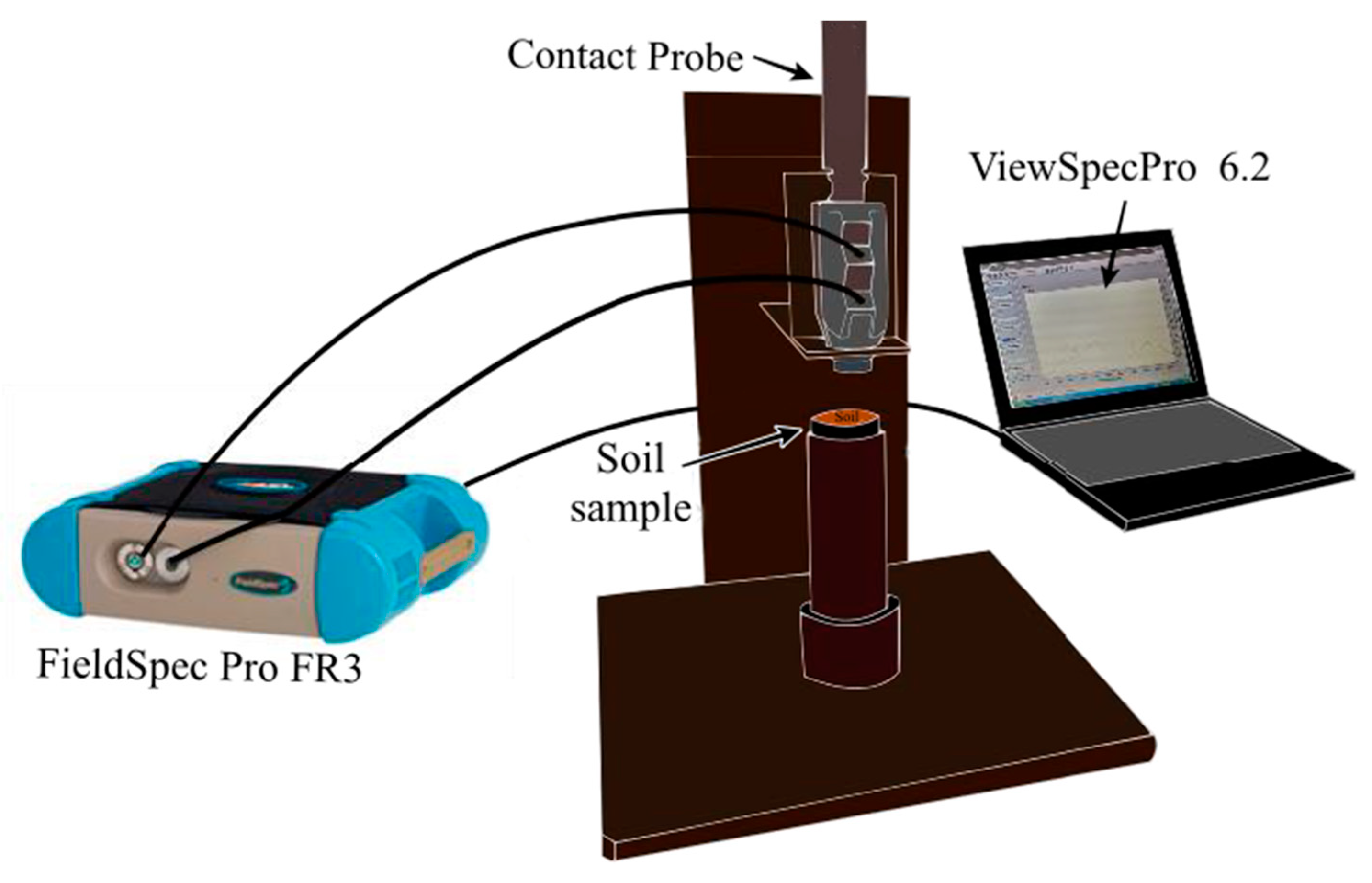
2.3. Acquisition of the Hyperspectral Data

The soil spectral data were obtained at the Geoprocessing Laboratory of the Agricultural Engineering Department of the Federal University of Ceará. Each soil sample was submitted to the oven-drying method at 45 °C and placed in a black polypropylene container, 5 cm in diameter and 15 mm in height.

Continuous spectral readings of the samples were taken in a darkroom in a climate-controlled environment, using a Hi-Brite Contact Probe together with a FieldSpec Pro FR3 spectrometer (350–2500 nm). This non-imaging sensor combines three spectrometers with spectral resolutions of 3 nm and 10 nm resampled to 1 nm, and performs real-time reflectance calculations with a 25° full-angle cone of acceptance field-of-view [55]. Sensor calibration (white reference) for the reflectance factors (ρ) was carried out every 20 min, using standard readings on a spectralon plate with characteristics similar to a Lambertian surface, in which 100% of the input energy is reflected in all directions [36].

Data were collected from three spectra at random points on the surface of the samples. Each point represented the arithmetic mean of 50 spectral readings, allowing every sample to be characterised by the total mean value (150 spectra/sample). Figure 3 shows the data acquisition geometry. The mechanism, employed by the authors, allowed the samples to be secured and stably elevated until in direct contact with the probe. The Digital Number (DN) values of the soil samples were converted into a reflectance factor using ViewSpecPro 6.2 software.

2.4. Quantification of the Soil Organic Carbon

The Soil Organic Carbon (SOC) in the samples was quantified in duplicate at the Soil–Water–Plant Relationship Laboratory of the Department of Agricultural Engineering, Federal University of Ceará. The soil samples were broken up, air dried, and sifted using a 2 mm mesh, then macerated in a porcelain mortar and passed through a mesh of 0.2 mm. The macerated samples were digested in potassium dichromate (K₂Cr₂O₇) and sulphuric acid (H₂SO₄) [98%], with an external heating source [15].

Air drying was only carried out for the chemical analysis of the samples, which were then not exposed to the spectroradiometer (Figure 4). The samples intended for spectral analysis were oven-dried (45 °C) to standardise their moisture conditions and reduce the vibration effect of the water molecules on the reflectance spectrum [56,57,58].

With the drying method (open-air or greenhouse), dissolved organic carbon is also evidenced, and the organic characteristics of the soil are preserved in the long term, as these tend to present different dynamics for different levels of moisture, such as in fresh samples [59,60].

2.5. Exploratory Data Analysis

Initially, a descriptive analysis of the carbon data was performed, including the mean, median, standard error of the mean, minimum and maximum values, standard deviation, variance, coefficient of variation, kurtosis, and asymmetry. The frequency distribution of the data and the normality hypothesis test were then analysed using the Kolmogorov–Smirnov test at 5%. To assess the linear intensity and the direction between the chemical and spectral variables of the samples, the Pearson linear correlation coefficient was used between the SOC content and the corresponding spectra, as well as their mathematical transformations, as per Equation (1):

$$r=\frac{{{\displaystyle \sum }}_{i=1}^n(x_i-x)(y_i-y)}{\sqrt{[{{\displaystyle \sum }}_{i=1}^n{(x_i-\overline{x})}^2][{{\displaystyle \sum }}_{i=1}^n{(y_i-\overline{y})}^2]}} ,$$

(1)

where r represents the Pearson correlation coefficient; x_i and y_i are the values measured in both variables (independent and dependent, respectively) for the i-th individual; and $\overline{x}$ and $\overline{y}$ represent the arithmetic mean of the respective variables.

2.6. Selection of the Significant Variables

As it presents a notably extensive set of independent variables (50 spectra × 2151 wavelength frames × 3 replicas × 65 samples = 2 × 10⁷ data points), the visible (VIS), near infrared (NIR), and short-wave infrared (SWIR) ranges were submitted to the Stepwise method to select the wavelengths with the greatest sensitivity to fluctuations in the SOC. This method was based on incrementing (forward) the most significant variables for the model, and on removing (backward) those that least represent the structure of the chemical data (SOC). By the end of the iterations, it was possible to reduce the dimensionality of the dataset, keeping the physical significance of the input variables.

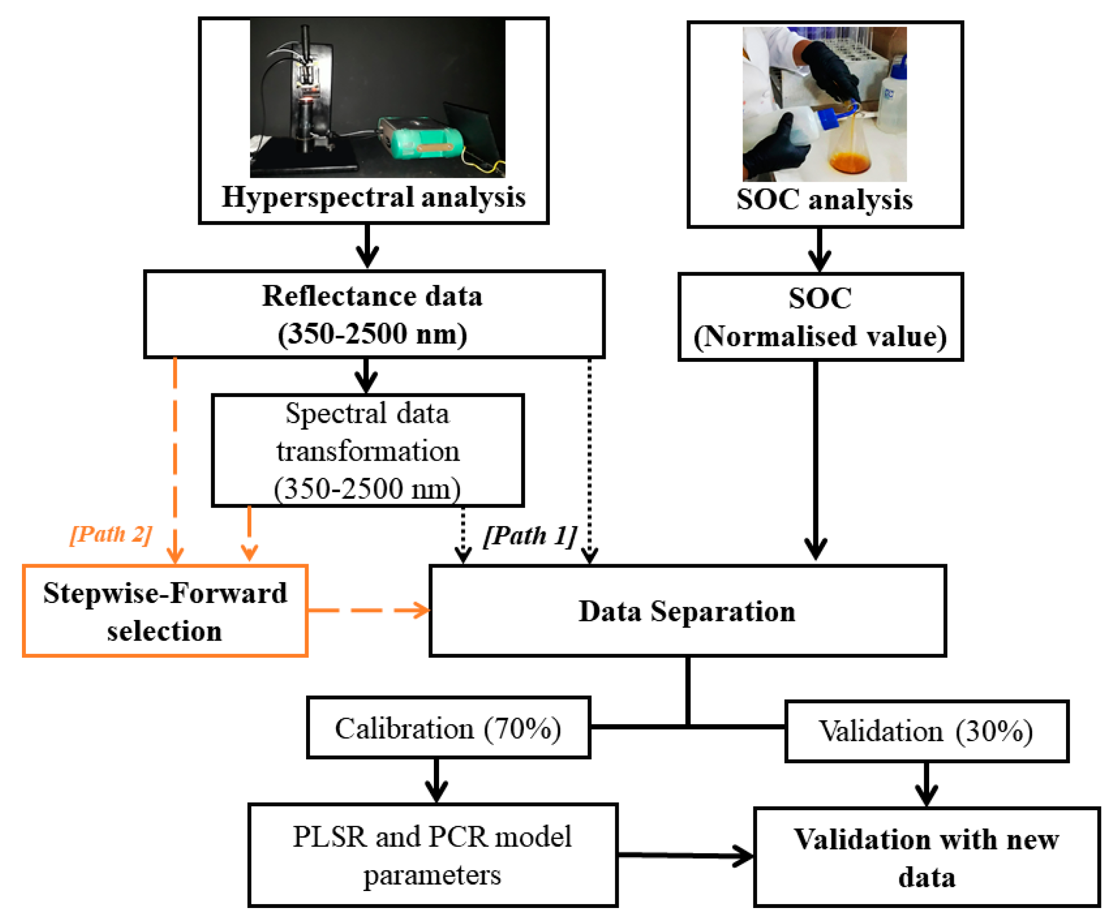
2.7. Treatment of the Hyperspectral Data

To construct the estimation models, in addition to the untransformed hyperspectral data, the data were transformed using: (i) the first derivative; and (ii) Savitzky–Golay smoothing.

2.7.1. First Derivative

The first-derivative technique for hyperspectral data offers the advantage of showing the variation in the reflectance of a target relative to the variation in wavelength, in addition to exposing noise that might be interpreted as a signal. Therefore, to facilitate understanding and observation of the enhancement of features in the sample spectra, the first derivative was calculated with a window (Δλ) of 3 nm, enough to show where there were more-marked changes between nearby wavelengths [61].

The mathematical basis of first-order derivative analysis (dρ_λ) is established by the change in reflectance (ρ_λ) as a function of the wavelength λ at a given point i. The derivative is numerically approximated using symmetric or central deference, expressed by the equation presented by Rudorff et al. [62]:

$$\frac{{\mathrm{d}\rho }_{\mathsf{\lambda }}}{\mathrm{d}x}\cong \frac{{\rho }_{i+1}{- \rho }_{i-1}}{2\Delta x} ,$$

(2)

where Δx represents the difference between two subsequent bands (Δx = [x_i+1] − [x_i−1]), where [x_i+1] > [x_i−1], ρ_i+1 refers to the reflectance factor of the point following i; and ρ_i−1 corresponds to the reflectance factor of the previous point to i.

2.7.2. Savitzky–Golay Smoothing

Smoothing, as described by Savitzky and Golay [63], seeks to reduce random noise and avoids the introduction of distortions in the spectral data, preserving the shape of the spectrum, as per Equation (3):

$$y_j^{*}=\frac{1}{N} {\displaystyle \sum }_{h=-k}^k{C}_h{y}_{j+h} ,$$

(3)

where $y_j^{*}$ is the new smoothed value; C_h represents the coefficients of the smoothing filter; N is the size of the smoothing window; and k is the number of neighbouring values on each side of j. A smoothing filter with a third-degree polynomial function and window with three spectral points was therefore used to transform the spectral data.

2.8. Calibration and Validation of the Predictive Models

The mathematical models for estimating SOC in soil samples using the principal wavelengths were based on Partial Least Squares Regression (PLSR) [64] and Principal Components Regression (PCR) [65]. The difference between the two multivariate methods is the basis for constructing the models. While PLSR decomposes both the dependent and independent variables into scores to maximise the correlation between them, PCR decomposes only the independent variables into principal components (PC) and correlates them with the variable to be estimated [3,66].

The SOC content was normalised using the Min-Max method (Equation (4)) to reduce nonconformity in the orders of magnitude between the model parameters:

$$n_i=\frac{x_i-\min (x)}{\max (x)-\max (x)} ,$$

(4)

where n_i represents the normalised value in the i-th observation; x_i is the value of the real variable x in the i-th observation; min (x) and max (x) are, respectively, the minimum and maximum values of variable x. The chemical and spectral data of the samples were evaluated separately by area of collection (A1; A2) and, later, aggregated into a single sample set (A1 & A2) to construct the estimation models. With this last approach, we evaluated the effectiveness of the SOC prediction by disregarding the chemical and spectral heterogeneity of the samples in both soils.

The PLSR and PCR models were initially calibrated and validated for all wavelengths using both transformed and untransformed reflectance (Figure 5, path 1), and then after selecting significant spectral bands for the same data treatments (Figure 5, path 2).

From each working set of data, 70% of the soil samples were selected for model calibration, while the remaining 30% were separated for the validation phase, according to Bushong et al. [67], obtaining the A1 & A2 calibration and validation sets by aggregating the respective sets of samples. A specific model was constructed for each dataset (A1; A2; A1 & A2) and for each spectral transformation.

The validation process for the tested models was implemented using statistical metrics: coefficient of determination (R²) (Equation (5)); adjusted coefficient of determination (R² adjust) (Equation (6)); Root Mean Square Error (RMSE) (Equation (7)); and the ratio of prediction deviation (RPD) (Equation (8)):

$${\mathrm{R}}^2=1-\frac{{{\displaystyle \sum }}_{i=1}^N{(Y}_i{-\widehat{Y}}_i{)}^2}{{{\displaystyle \sum }}_{i=1}^N{(Y}_i-\overline{Y}{)}^2},$$

(5)

$${\mathrm{R}}_{\mathrm{adj}.}^2=1-\frac{(N-1)({1-\mathrm{R}}^2)}{N-(k+1)},$$

(6)

$$\mathrm{RMSE}=\sqrt{\frac{{{\displaystyle \sum }}_{i=1}^N{(\widehat{Y}}_i{-Y}_i{)}^2}{N}} ,$$

(7)

$$\mathrm{RPD}=\frac{{\mathsf{\sigma }}_{\mathrm{Yo}}}{\mathrm{RMSE}} ,$$

(8)

where Ŷ represents the values estimated by the models in the i-th observation; Y_i are the values measured or observed in the laboratory in the i-th observation; $\overline{Y}$ represents the mean of the observed values; N is the number of observations; k is the total of independent variables; and σ is the standard deviation for the measured values.

3. Results

3.1. Descriptive Statistics

The descriptive statistics for the organic carbon content of the samples of Fulvic Neosol and Haplic Cambisol, respectively, are shown in

Table 2. Descriptive statistics for the SOC content of the data, separated by area of collection (A1; A2) and unified into one set (A1 & A2).

Soil Organic Carbon (g/kg)
Statistical Parameters	A1	A2	A1 & A2
Mean	16.86	23.30	20.43
Standard error	1.64	0.91	0.97
Median	16.77	23.71	20.72
Standard deviation	8.84	5.48	7.81
Coefficient of variation (%)	52.42	23.50	38.23
Sample variance	78.16	29.98	60.99
Curtosis	2.19	−0.52	0.49
Assimetry	1.07	0.03	0.16
Amplitude	39.46	22.95	39.46
Minimum	5.74	13.41	5.74
Maximum	45.20	36.36	45.20
Kolmogorov-Smirnov (p-value)	0.561	0.693	0.510
Normality	Normal	Normal	Normal
Count	29	36	65

, by collection area of the soil samples (A1 and A2), and for the joint dataset (A1 & A2). It can be seen that the mean and median values for SOC—in the three data sets—are relatively close, suggesting that the central trend estimators are typical of a normal distribution [68]. As shown by the Kolmogorov–Smirnov test at 5%, the data showed low distortion, where the SOC values for the data sets featured a p-value > 0.2, underlining their normality.

It can be seen from the statistical parameters that for the SOC content, the samples from A1 are different to those from A2. This contrast influenced the statistical evaluation when the data from the two soils were observed together (A1 and A2). Such behaviour is seen when evaluating the asymmetry coefficient for the three data sets. This coefficient was more prominent in the samples of A1 soils (|AS| = 1.07), since there were values above the mean, with a peak of 45.20 g kg⁻¹ SOC. This exerted a significant effect on the mean of the distribution, albeit for a single occurrence [69,70]. As a grouped set (A1 and A2), the data distribution of A1 was influenced by the asymmetry of the A2 samples (|AS| = 0.03 resulting from values above the mean (|AS| = 0.16), with a consequent reduction in the coefficient.

The same can be seen with the coefficient of variation (CV) where, for the samples from A1 and A2, the SOC content showed a variation of 52.42% and 23.50%, respectively, while the data from A1 & A2 showed a coefficient of 38.23%. This result shows that the variability in SOC content from A1 and A2 separately changes when the data becomes part of the joint A1 & A2 group, showing the statistical influence of one dataset over the other.

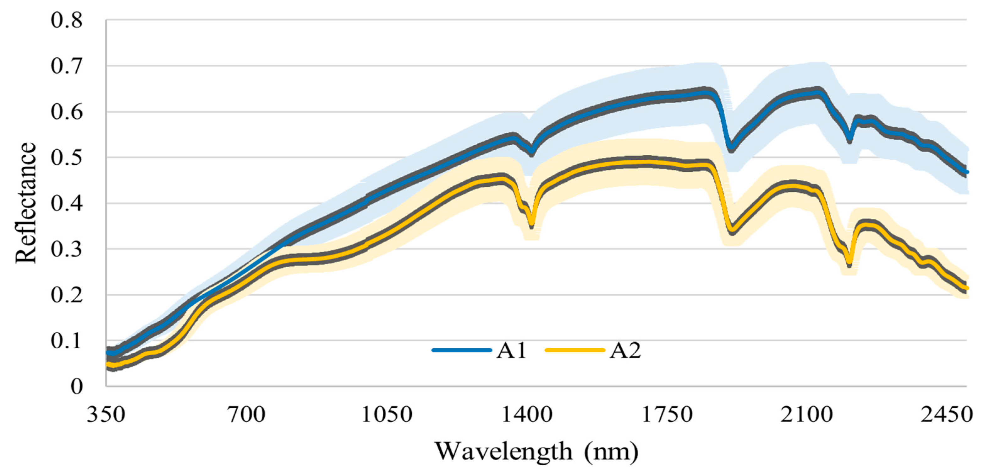
3.2. Analysis of the Hyperspectral Data

For the spectral behaviour of the soil samples under evaluation, Figure 6 shows a marked change in the mean spectral signature between the soils of A1 and A2.

Analysing the spectral profiles of two samples collected in A2, the strong influence of the increase in SOC content can be seen by a reduction in reflectance in the spectrum from 350 nm to around 2000 nm. Figure 7 shows that, even with a higher content, the sample with 36.36 g kg⁻¹ SOC presents a marked brightness, which is not that different from the sample containing a smaller amount of carbon (13.41 g kg⁻¹). It is worth noting that, in addition to the SOC content, the mineralogy, such as the kaolinite and iron oxides present in the soils of this region, also influences the spectral response of samples [71].

In Figure 8, the mean spectral behaviour of the soils of A1 and A2 is displayed in the form of reflectance (Figure 8a), first derivative (Figure 8b) and smoothed reflectance (Figure 8c). Reflectance smoothing shows no significant changes in relation to the untransformed spectrum. On the other hand, the first derivative shows the points in the spectrum where there were fluctuations.

The first derivative transformation of reflectance (Figure 8b) highlights the points where there are sudden changes in the spectral response, whose positive and negative peaks are related to the consecutive slopes of reflectance and absorption, respectively, in the original spectrum [72]. The values closest to the abscissa (zero value) correspond to points of continuity in the spectral pattern [73].

It was found that the behaviour of the first derivative in A2 differs from that of A1 between 450 nm and 1000 nm, showing more pronounced fluctuations in A2. This can be explained by the spectral variation due to the presence of iron oxides in the soils of this area, showing that the first derivative transformation is efficient at highlighting components of lower intensity that help to make up the sample. The unusual peak between 1000 and 1001 nm in the first derivative punctuates the noise caused by sensor transition in the region of the near infrared, intrinsic to the data acquisition equipment [36].

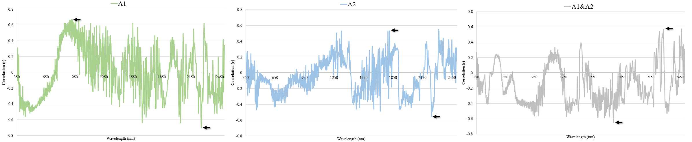
3.3. Pearson Correlation Coefficients

The first derivative transformation of reflectance was the spectral treatment that showed the best correlations between the SOC content and the wavelength across the entire spectrum (Figure 9). After removing any effects of noise at the extreme values (around 350 nm and 2500 nm), the variation in SOC content was better correlated with wavelengths close to 2200 for the all the data sets, with highlights at 897 nm in A1, 1797 nm in A2, and 1762 nm in A1 & A2 (Figure 9).

Wavelengths at 2300 nm are associated with aromatic groups or aliphatic carboxylic bonds related to the actual structure of the organic matter associated with mineral particles in the soil [74], while absorption troughs at 700 nm [75] are related to the influence of organic carbon and humic acids, in addition to an absorption feature at 1700 nm, which is important for predicting C-H bonds present in the structure of organic matter [76].

In A1, the bands from 750 nm to 1000 nm showed a constant positive correlation with the SOC concentrations (Figure 9a), with approximately r = 0.6 in the 900 nm region; the same occurred with the samples from A2 in the 1400 nm and 1900 nm region. For A1, the 2259 nm wavelength showed a strong negative correlation (r = −0.70) with the SOC content of the samples, while for A2, the 2241 nm band showed a moderate correlation (r = −0.56). Meanwhile, using the joint data from the two areas (A1 & A2), the 1762 nm wavelength also showed a strong negative correlation with the SOC concentrations (r = −0.65).

3.4. Full-Spectrum Estimation of SOC Content

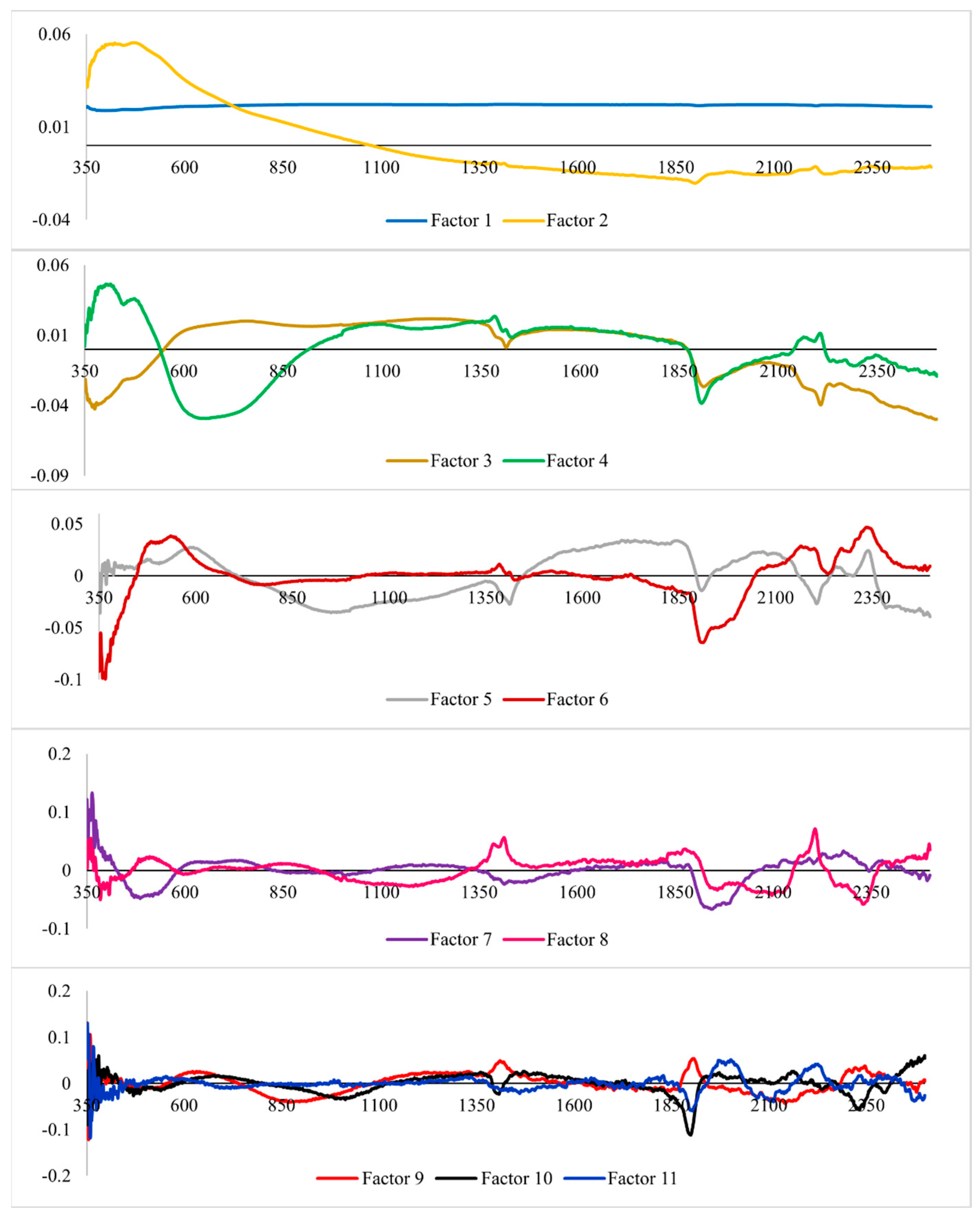
3.4.1. Principal Component Regression (PCR)

Initially, the prediction models using principal component regression (PCR) were constructed using all the bands and the following spectral treatments: (i) untransformed reflectance data; (ii) first derivative; and (iii) Savitzky–Golay smoothing (

Table 3. Validation results of the PCR models for estimating SOC using the 350–2500 nm spectrum.

Sample	Spectral Data	Nbr of Factors	R2 Calib.	R2 Valid.	Adj. R2 Valid.	RMSE (Norm)	Standard Dev.	RPD
A1 (20/9)	Untransformed	11	0.78	0.86	0.84	0.152	0.31	2.03
	First derivative	17	0.99	0.91	0.90	0.176	0.31	1.76
	Smoothed reflectance	11	0.78	0.86	0.84	0.150	0.31	2.06
A2 (25/11)	Untransformed	19	0.96	0.40	0.34	0.217	0.28	1.30
	First derivative	5	0.59	0.13	0.03	0.257	0.28	1.10
	Smoothed reflectance	20	0.95	0.39	0.32	0.221	0.28	1.28
A1 & A2 (45/20)	Untransformed	26	0.89	0.77	0.76	0.106	0.22	2.11
	First derivative	1	0.55	0.17	0.13	0.292	0.22	0.77
	Smoothed reflectance	20	0.84	0.73	0.72	0.116	0.22	1.93

).

It should be noted that for A1, the strategies with the untransformed and smoothed data stood out in relation to the models with unified A1 & A2 data due to the need for a reduced number of factors. This is because, despite featuring the highest RPD (2.11), the PCR model using the A1 & A2 data required 26 components to estimate the SOC with an adjusted R² of 0.76. The SOC prediction with the samples from A1 showed no significant differences when using untransformed or smoothed spectral data, with an adjusted validation R² of 0.86 and R² of 0.84. Furthermore, they presented the same number of factors for constructing the models, the only differences being the RMSE of 15% and the RPD of 2.06.

The PCR loadings that demonstrate the contributions of each wavelength to the variability of the smoothed spectral data in A1 are shown in Figure 10. The first factor, corresponding to the changes in brightness across the spectrum [77], showed the constant influence of each spectral band (350–2500 nm), while the bands in the region of 350–900 nm contributed significantly to the second factor (Figure 10). These same wavelengths contribute to factor 4, positively up to 550 nm and then negatively up to 900 nm; this region can be considered more influenced by organic matter (OM) and iron oxides [78].

It should also be noted that factor 3 receives a constant contribution from the wavelengths at 550–1400 nm (Figure 10). A part of these wavelengths that are distributed over the visible region is usually associated with the amine functional groups of soil organic matter [79] and with the colour of the soil [80]. The 1900 nm wavelength features the greatest contribution to factors 6 and 7. This spectral region has previously been reported as sensitive to organic matter [81]. The wavelengths at 1400 nm and 2200 nm exerted a positive influence on the eighth factor, while a negative contribution can be seen at 2300 nm, which is cited as an important zone for the SOC concentration [74]. The final latent variables represented noise more strongly, especially at the initial end of the spectrum, except for factors 9 and 10, again with a greater contribution at 1900 nm.

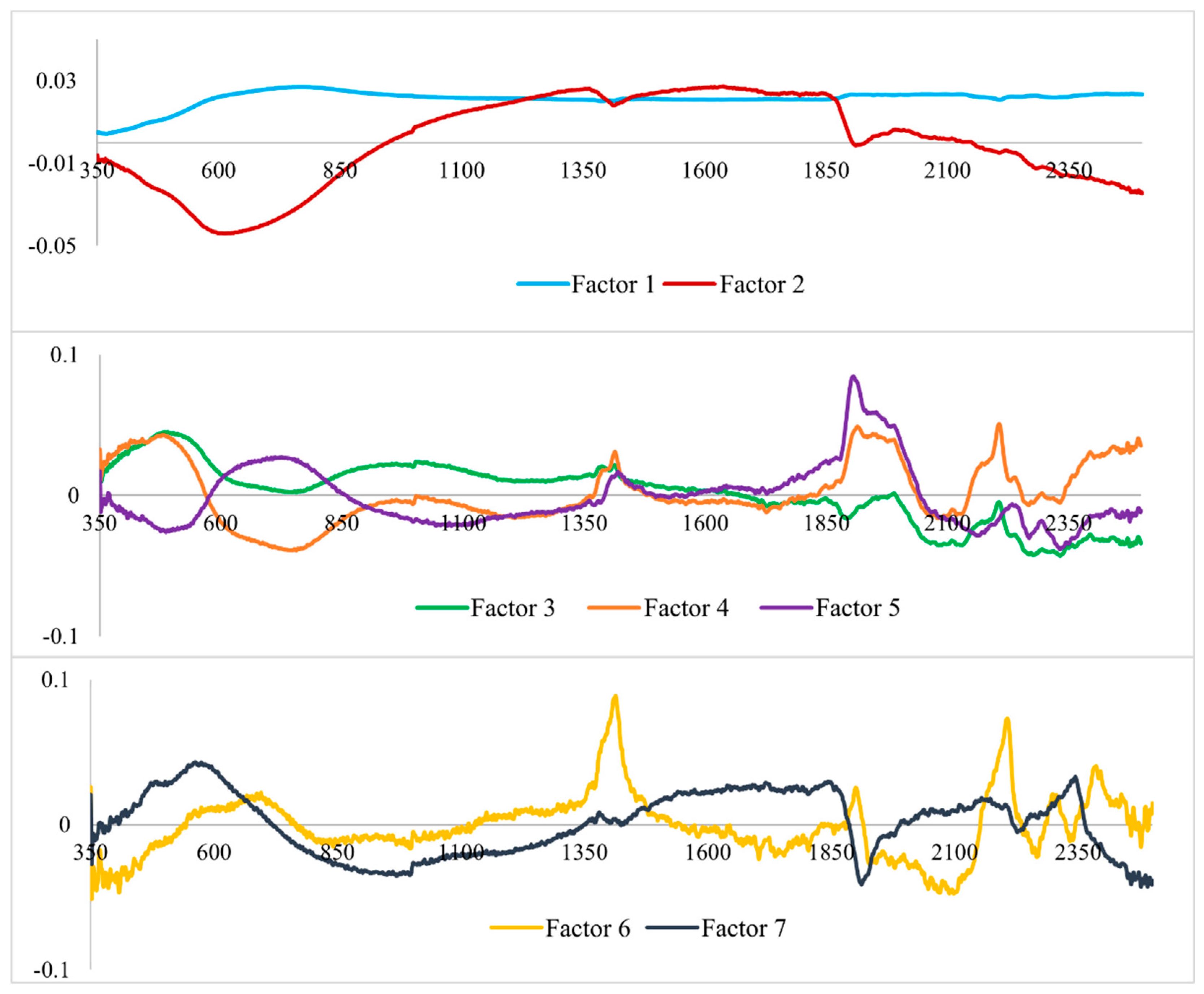
3.4.2. Partial Least Squares Regression (PLSR)

In a similar way to the PCR, the PLSR was performed using all the spectral bands with untransformed reflectance data and their transformations (first derivative and Savitzky–Golay smoothing). After obtaining the estimation models by PLSR, they were tested with the unused data in a pure validation. The results are shown in

Table 4. Validation results for the PLSR models for estimating SOC using the 350–2500 nm spectrum.

Sample	Spectral Data	Nbr of Factors	R2 Calib.	R2 Valid.	Adj. R2 Valid.	RMSE (Norm)	Standard Dev.	RPD
A1 (20/9)	Untransformed	8	0.87	0.81	0.78	0.150	0.31	2.07
	First derivative	6	0.98	0.88	0.86	0.160	0.31	1.93
	Smoothed reflectance	7	0.78	0.84	0.81	0.151	0.31	2.04
A2 (25/11)	Untransformed	11	0.98	0.44	0.38	0.223	0.28	1.27
	First derivative	1	0.98	0.07	0.02	0.292	0.28	0.97
	Smoothed reflectance	11	0.96	0.47	0.41	0.218	0.28	1.29
A1 & A2 (45/20)	Untransformed	12	0.89	0.73	0.71	0.119	0.22	1.88
	First derivative	1	0.61	0.19	0.14	0.302	0.22	0.74
	Smoothed reflectance	13	0.88	0.76	0.75	0.112	0.22	1.99

.

Spectrum smoothing can improve model performance, as per the report by Mousavi et al. [82], and can be seen in the A2 and A1 & A2 sample subsets. This strategy reduced the random noise existing in the original data and, as a result, increased the signal/noise ratio in the spectra. For A1 especially, the use of smoothed reflectance reduced the number of factors and improved the validation R² (0.84) and adjusted validation R² (0.81). Despite reducing its performance (RPD = 2.04) and presenting an RMSE of 15.1%, the PLSR with the smoothed spectrum ensured that the model was classified as excellent, agreeing with Chang et al. [83].

For A2, spectrum smoothing improved the performance of the PLSR, but was not enough to construct suitably valid models for predicting the SOC; as each spectral treatment shows an RPD < 1.4, models for A2 using all the spectral bands can be considered inefficient. Smoothing was also able to improve the prediction performance of the model when using the complete subset of samples, generating an RPD of 1.99, which is considered a reliable prediction model open to new approaches for improving the fit. Therefore, using all the bands in the spectrum, A1 presented better-performing models for predicting SOC using PLSR, which was probably due to the fact that these samples showed greater variability. In this study, it was found that the models better fitted the sample subsets that showed greater variation in chemical concentration in the validation data compared to the calibration data.

The spectral variables feature different weights for forming each latent variable (factor). As such, Figure 11 shows the loadings that allow the spectral bands to be identified that best contributed to each factor of the model constructed for A1 using the smoothed spectral data. It can be seen that the region comprising 350 nm to 900 nm—under the strong influence of organic matter—made a significant contribution to each factor. These results are corroborated by Zhang et al. [84], who highlight the greater association of these wavelengths with the organic matter content of soil.

Clearly, factor 1 is directly related to reflectance throughout the spectrum (350–2500 nm), with an almost constant contribution at all wavelengths (BRIGHTNESS), as seen in studies by Rocha Neto et al. [77]. As the first latent variable, factor 1 was the most representative of the variation in spectral data at all wavelengths, which relates it to the changes in albedo, representing general reflectance in the 400–2500 nm range [85].

From the second factor onwards, all the latent variables contributed to spectral variability around the visible region, in addition to the region between 1450 and 1880 nm, which also positively influenced this latent variable. The wavelengths of 1400 nm, 1900 nm and 2200 nm, regions of marked absorption peaks of the hydroxyl group (OH) and clay minerals [75,86], also exerted a strong influence on factors 4, 5 and 6. Factor 7 was influenced by peaks in the visible region (350–600 nm) and at 1400 nm.

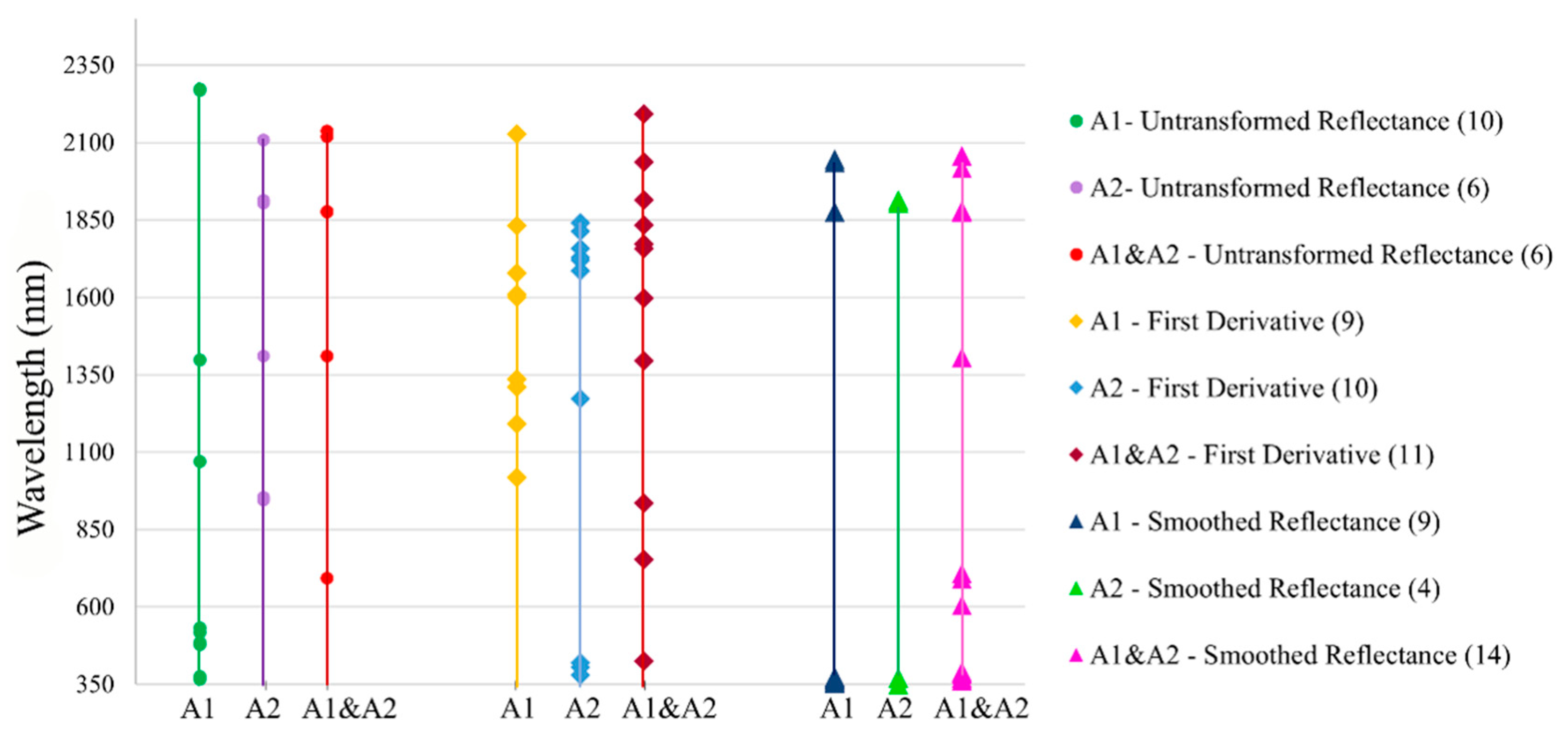
3.5. Selection of Significant Bands

For all the spectral treatments, the most relevant bands were selected using the Stepwise Forward method, in order to identify the bands that best represent the variation in SOC content. Figure 12 shows these wavelengths for each sample subset and spectral treatment. In general, this method selected spaced spectral bands between the visible and shortwave infrared region, determining a minimum of four bands using the samples from A2 with a smoothed spectrum, and a maximum of 14 bands using all the samples with the same spectral treatment.

Examining the untransformed dataset, it can be seen that the method allowed a well-distributed selection throughout the range under analysis (350–2500 nm). The relevance of the wavelengths around 1400 nm in representing the variance seen in the SOC should be noted, a fact shown by the three sample subsets (Figure 12). This is due to the absorption peak in this region of the spectrum that results from the influence of combinations of the hydroxyl group (O-H) with the mineralogy of the sample [86].

The wavelengths between 1600–1800 nm, evidenced by the first derivative for all the sample sets, are normally associated with the SOC due to vibrations of the C-H bonds found in the structure of organic matter, especially around 1700 nm [76,87]. Wavelengths at 1720 and 1760 nm, selected using soil samples from A2, and from the A1 & A2 data set, are also able to demonstrate the influence of aliphatic carboxylic bonds, the main sources of carbon present in organic matter [79,88].

With spectrum smoothing, wavelengths were clearly shown in the visible region, and around 1800 nm when evaluating the spectrum of the A1 and A2 samples separately. Discrete absorption peaks in the 350–700 nm region are related to the presence of carbon in darker organic compounds, such as humic acids; it is therefore common that wavelengths in this region can be evidenced by their influence on the colour of the samples [80]. The same was seen when using the unified A1 & A2 samples, with the addition of 1400 and 1900 nm, which were possibly influenced by hydroxyl vibration in the samples.

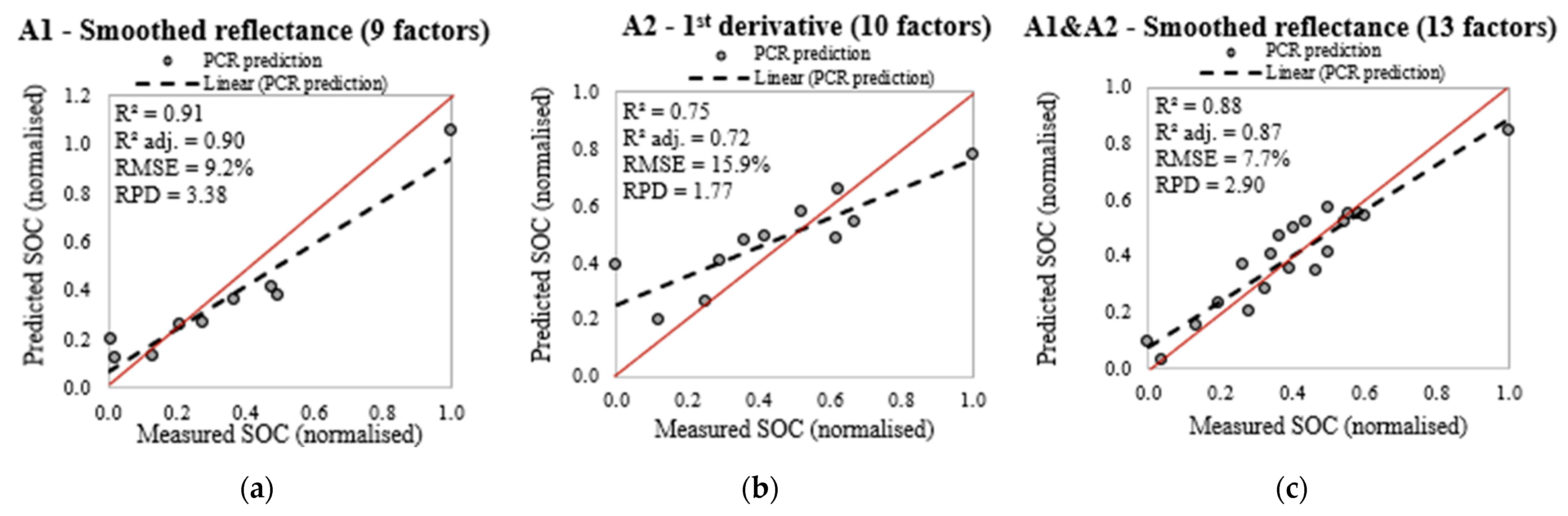
3.5.1. Principal Component Regression after Band Selection

Based on the selection of spectral bands that best represent the variation in the SOC data, prediction models were constructed using PCR, including all the spectral treatments already mentioned, and the wavelengths with the best performance in each treatment. The models that were constructed using only the bands selected by the Stepwise Forward method improved SOC prediction for each treatment of the spectral data, as shown in

Table 5. PCR models for SOC prediction after selecting the spectral bands.

Sample	Spectral Data	Nbr of Factors	R2 Calib.	R2 Valid.	Adj. R2 Valid.	RMSE (Norm)	Standard Dev.	RPD
A1 (20/9)	Untransformed	10	0.97	0.96	0.96	0.117	0.31	2.65
	First derivative	10	0.72	0.90	0.89	0.108	0.31	2.85
	Smoothed reflectance	9	0.90	0.91	0.90	0.092	0.31	3.38
A2 (25/11)	Untransformed	5	0.62	0.61	0.57	0.181	0.28	1.56
	First derivative	10	0.82	0.75	0.72	0.159	0.28	1.77
	Smoothed reflectance	4	0.46	0.61	0.56	0.202	0.28	1.40
A1 & A2 (45/20)	Untransformed	6	0.74	0.71	0.70	0.118	0.22	1.90
	First derivative	11	0.86	0.82	0.81	0.102	0.22	2.19
	Smoothed reflectance	13	0.86	0.88	0.87	0.077	0.22	2.90

.

By using only samples from A1, each model for each spectral treatment proved to be efficient at predicting the SOC using selected bands, with an adjusted validation R² ranging from 0.89 to 0.96 and RPD between 2.65 and 3.38. The reduction in RMSE in all the prediction models shows that band selection was efficient in improving performance. The best estimation model, using samples from A2, was the model in which the reflectance factors were transformed using the first derivative. Despite being composed of 10 latent variables, the model showed reliable performance, with an adjusted validation R² of 0.72 and the lowest RMSE (15.9%), based on the RPD for the model of 1.77.

When constructing the predictive models using the A1 & A2 data, the least efficient, albeit reliable, was the prediction that included reflectance, with an adjusted validation R² of 0.70 and RPD of 1.90. Savitzky–Golay reflectance smoothing improved the prediction performance after band selection, presenting an RPD of 2.90 and an adjusted validation R² of 0.87.

Table 6. Equations for SOC prediction (g kg⁻¹) with the best models constructed using PCR for each sample subset, including the respective adjusted R².

Sample	Spectral Data	Best SOC Prediction Models	Adj. R2
A1	Smoothed reflectance	Y = 33.62032 + 1005.37 (ρ 1876 nm) − 2749.841 (ρ 2047 nm) + 3447.796 (ρ 369 nm) − 3087.381 (ρ 354 nm) − 1961.023 (ρ 361 nm) − 2416.18 (ρ 366 nm) + 2568.7 (ρ 355 nm) + 1783.143 (ρ 2037 nm) + 1103.126 (ρ 375 nm)	0.90
A2	First derivative (ρ’)	Y = 7.1693 + 42,200.559 (ρ’ 1813 nm) + 26,103.8192 (ρ’ 1840 nm) − 7700.9938 (ρ’ 419 nm) – 17,267.2974 (ρ’ 1719 nm) + 32,662.4702 (ρ’ 1273 nm) + 14,296.5261 (ρ’ 406 nm) + 2574.3248 (ρ’ 1685 nm) – 18,546.4386 (ρ’ 1757 nm) + 3891.96 (ρ’ 380 nm) + 5449.9437 (ρ’ 1728 nm)	0.72
A1 & A2	Smoothed reflectance	Y = 15.3110 − 816.0873 (ρ 2057 nm) + 4177.451 (ρ 370 nm) + 408.1595 (ρ 605 nm) + 770.9059 (ρ 1876 nm) + 2420.435 (ρ 390 nm) − 758.8688 (ρ 362 nm) + 317.3015 (ρ 1406 nm) + 288.1545 (ρ 2018 nm) − 1810.411 (ρ 371 nm) − 776.0894 (ρ 691 nm) − 2994.089 (ρ 388 nm) − 958.5162 (ρ 381 nm) + 297.9998 (ρ 708 nm) − 442.805 (ρ 1880 nm)	0.87

shows the equations for the PCR models with the best performance in predicting SOC (g kg⁻¹), including the bands selected in each spectral treatment and their respective coefficients restored to non-normalised values.

PCR performed better when using smoothed spectral data for the samples from A1 and A1 & A2, and with the first derivative for samples from A2 (Figure 13 and Tables S1–S4). For the prediction models that used the smoothed spectrum, the most significant wavelengths are found between 354 and 375 nm and in the 1876 nm, 2037 nm and 2047 nm bands for A1, while using joint sample data from the two areas, A1 & A2, the spectral range was extended to include the wavelengths at 362–390 nm, 605–708 nm, 1406 nm, 1876 nm, 1880 nm, 2018 nm and 2057 nm. This expansion of the most significant spectral range for SOC prediction in the complete subset of samples, may be related to the variation in the structural characteristics of the samples in the subset, as they come from different types of soil with different carbon-associated chemical patterns that respond in different spectral bands.

By using only the samples from A2 with the first derivative transformation of the reflectance, the prediction models using the selected spectral bands showed wavelengths around 400 nm, 1273 nm, 1685 nm, 1740 nm, 1813 nm, and 1840 nm.

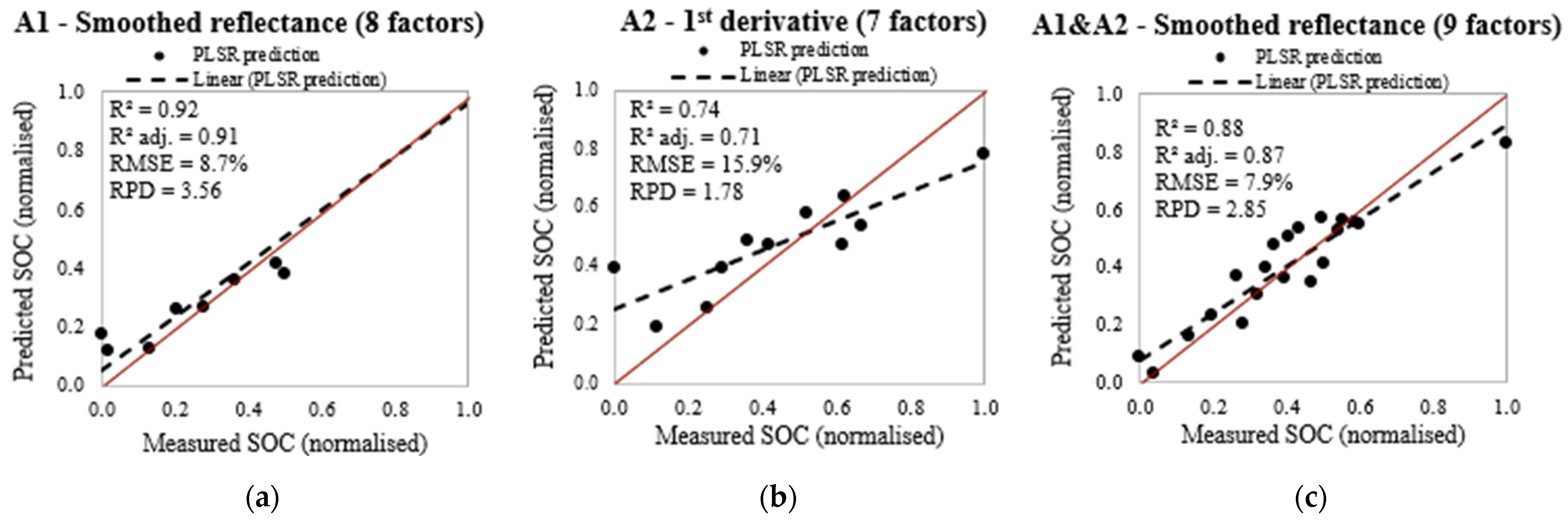
3.5.2. Partial Least Squares Regression after Band Selection

As with PCR, constructing predictive models using PLSR improved performance in estimating the SOC. The improvement in performance can be seen in

Table 7. PLSR models for SOC prediction after selecting the spectral bands.

Sample	Spectral Data	Nbr of Factors	R2 Calib.	R2 Valid.	Adj. R2 Valid.	RMSE (norm)	Standard Dev.	RPD
A1 (20/9)	Untransformed	9	0.95	0.95	0.95	0.141	0.31	2.19
	First derivative	9	0.72	0.90	0.89	0.109	0.31	2.85
	Smoothed reflectance	8	0.90	0.92	0.91	0.087	0.31	3.56
A2 (25/11)	Untransformed	5	0.62	0.61	0.57	0.182	0.28	1.56
	First derivative	7	0.81	0.74	0.71	0.159	0.28	1.78
	Smoothed reflectance	4	0.46	0.61	0.56	0.202	0.28	1.40
A1 & A2 (45/20)	Untransformed	6	0.74	0.71	0.70	0.118	0.22	1.90
	First derivative	7	0.86	0.86	0.85	0.097	0.22	2.30
	Smoothed reflectance	9	0.83	0.88	0.87	0.079	0.22	2.85

, where the relevance of selecting significant hyperspectral variables can be seen.

Band selection improved the performance of the prediction models for all the sample subsets and using all the spectral treatments under analysis, besides reducing the number of factors needed to estimate SOC using PLSR. The prediction models constructed using only the samples from A1 demonstrated an adjusted validation R² of between 0.89 and 0.95, RMSE of 8.7% and 14.1%, and minimum RPD of 2.19 and maximum of 3.56, all considered excellent [83].

The models constructed for A2 became reliable after band selection, but still required fine-tuning to make better SOC predictions. The first derivative transformation of reflectance afforded the best predictions, with seven factors and an adjusted validation R² of 0.71; the best RPD for A2 was 1.78, with the possibility of further optimisation.

For the A1 & A2 subset, the first derivative transformation of the spectral data and the data smoothed using Savitzky–Golay exhibited an excellent prediction performance, with an RPD equal to 2.30 and 2.85, respectively, and an adjusted validation R² ranging from 0.85 to 0.87. The most suitable prediction model can be defined as the model that demonstrates the best performance (RPD ≥ 2.0) and succeeds in estimating organic carbon with the lowest prediction error. It should be noted that using the joint sample data, the smoothed spectrum generated the best SOC prediction model, with an RMSE equal to 7.9%.

Table 8. Equations for SOC prediction (g kg⁻¹) with the best models constructed using PLSR for each sample subset, including the respective adjusted R².

Sample	Spectral Data	Best SOC Prediction Models	Adj. R2
A1	Smoothed reflectance	Y = 33.11747 + 1056.97 (ρ 1876 nm) − 2634.573 (ρ 2047 nm) + 3390.864 (ρ 369 nm) − 3108.625 (ρ 354 nm) − 2379.895 (ρ 361 nm) − 2363.19 (ρ 366 nm) + 2709.004 (ρ 355 nm) + 1617.641 (ρ 2037 nm) + 1393.959(ρ 375 nm)	0.91
A2	First derivative (ρ’)	Y = 7.0083 + 42,065.0622 (ρ’ 1813 nm) + 25,818.0458 (ρ’ 1840 nm) − 7725.9588 (ρ’ 419 nm) − 17,941.3756 (ρ’ 1719 nm) + 31,823.2575 (ρ’1273 nm) + 15,099.1473 (ρ’ 406 nm) + 1880.134 (ρ’1685 nm) – 16,964.3115 (ρ’ 1757 nm) + 3299.873 (ρ’ 380 nm) + 5051.7084 (ρ’ 1728 nm)	0.71
A1 & A2	Smoothed reflectance	Y = 17.0995 − 741.6441 (ρ2057 nm) + 4471.37 (ρ370 nm) + 364.3325 (ρ605 nm) + 639.766 (ρ1876 nm) + 2839.064 (ρ390 nm) − 932.5751 (ρ362 nm) + 294.2628 (ρ1406 nm) + 163.4081 (ρ2018 nm) –2184.5980 (ρ371 nm) − 738.3680 (ρ691 nm) − 3583.7460 (ρ388 nm) –549.9565 (ρ381 nm) + 306.6913 (ρ708 nm) − 248.5569 (ρ1880 nm)	0.87

shows the equations formulated in constructing the best models, with the coefficients returned to the non-normalized scale and the most representative wavelengths for SOC prediction (g kg⁻¹) using PLSR.

Various bands in the visible region were selected using the Stepwise Forward method for the three models showing the best prediction performance (Figure 14 and Tables S1–S4), confirming the influence of SOC on the region of the spectrum between 350 and 720 nm.

In general, the predictive models constructed using the soil samples from A1 proved to be more efficient at estimating SOC for both multivariate methods under evaluation. This behaviour was noteworthy both before and after the selection of more significant spectral bands. Figure 15 shows the variation in the RMSE error metric as the number of factors was increased in the PCR and PLSR models for the three spectral treatments.

During the search for the subsets with the best characteristics for constructing the A1 models, the RMSE values were the lowest when up to 10 factors were required using PCR (Table 5) and PLSR (Table 7) after selecting the variables, as well as the full-spectrum PLSR model (Table 4). The exception was when constructing the full-spectrum PCR model (Table 3), when more factors were used. This superiority was even more marked when using data transformed by the first derivative, which required 17 factors for a minimum RMSE of 0.176.

4. Discussion

4.1. Descriptive Statistics

The coefficient of variation found for the SOC content (g kg⁻¹) shows moderate data variability (12 ≤ CV ≤ 60), according to the classification by Campanha et al. [81]. Although A1 stands out in terms of data heterogeneity, this characteristic is reduced when grouping the chemical data into a single sample set (A1 & A2), where the more homogeneous SOC values of A2 have a general influence on the variation in the data. The same situation can be seen when analysing the standard deviation of the subsets.

The coefficients of kurtosis and skewness can be considered the most sensitive for observing the distribution of the data when there are extreme values relative to the mean and standard deviation, given that a single value can strongly influence these coefficients [89]. This was seen in the SOC content for A1, as shown in Table 2, where the maximum and discrepant value of 45.2 g kg⁻¹ is highlighted, a fact that increased the asymmetry.

4.2. Hyperspectral Data Analysis

The average spectral behaviour of the soils under evaluation (Figure 6) is consistent with the mean SOC content for the two regions, where A1 displayed a lower mean SOC compared to the mean for A2 (Table 3), which explains the tendency for A1 soils to feature higher reflectance factors. The increasing continuity of the mean reflectance in the VIS-NIR region in the spectral response of A1 soils, shown in the characteristic troughs, may have been the effect of SOM in the samples, even in small quantities. The results agree with the research carried out by Pearlshtien and Ben-Dor [78], who noted the effect of increased organic matter content on a reduction in the reflectance factors of soil samples.

The troughs shown between wavelengths from 450 nm to 950 nm in the mean spectral response of the samples collected in A2 may be related to the strong presence of different forms of iron, corroborating the results presented by various authors [52,71,90] who found the predominance of both amorphous and crystalline iron in Haplic Cambisols predominant in the region of A2. Iron oxides can take the form of goethite and hematite, which respectively influence the troughs seen between 480 nm and 530 nm, as noted by Demattê et al. [22].

According to Dalmolin et al. [91], a content of more than 17.0 g kg⁻¹ of soil organic matter negates the effect of iron oxides on the reflectance and colour of soil, the effect being stronger in the visible region. This behaviour, as described by the authors, can be seen in Figure 7, where a difference of 22.95 g kg⁻¹ in the SOC content between two samples of the same type of soil demonstrated the masking effect of carbon on the absorption troughs of oxides [78] up to around 2000 nm and, especially in the VIS-NIR region.

According to Mulder et al. [92], dark soils typically contain more OM than light soils, reflecting the effect of the carbon content on the composition of the sample together with the change in spectral behaviour. This effect can be seen in Figure 7, where the sample with the highest SOC content (36.36 g kg⁻¹) features a darker colour and reduced reflectance, with smoothing of the characteristic iron oxide troughs. The opposite can be seen in the spectral behaviour of the sample with the reduced SOC content (13.41 g kg⁻¹), showing evidence of characteristic iron oxide troughs in the VIS-NIR region. Absorption curves characteristic of the presence of iron oxides and organic matter were also observed by Hong et al. [93] in the region between 480 and 900 nm.

The first-derivative transformation of reflectance for the soil samples from A2 shows discrepant peaks close to 1400, 1990, and 2200 nm (Figure 8b), the first two peaks being closely related to the hydroxyl groups and moisture between the layers of clay minerals [20,94], while the spectral band at 2200 nm is closely related to the presence of 2:1 clay minerals or kaolinite, which are able to form strong bonds with the OM, protecting any SOC [95].

The absorption peaks at 1400 and 1900 nm should be considered in spectral data acquired in the laboratory as they indicate the water remaining in a controlled environment; however, unless one is using a Hi-Brite probe type, they cannot be used in field analysis or by satellite images due to the influence of in situ atmospheric moisture.

4.3. Correlation between the Variation in Soc and the First Derivative of Reflectance

It should be noted from Figure 9a that the first derivative of the reflectance around 950 nm was positively correlated with the variation in SOC of the samples from A1 (r = 0.60), while the 2259 nm wavelength exhibited a strong negative correlation (r = −0.70) with the carbon of the samples, as well as with the soil samples from A2, which presented a marked correlation at 2241 nm (r = −0.56). These results corroborate the studies of Vohlad et al. [96], who identified the absorption region around 2200 nm as relevant for the purposes of predicting soil carbon, whereas Rinnan and Rinnan [97], using first derivative transformation, found that the region from 2040 nm to 2260 nm exerted the most influence when estimating the soil carbon.

A similar result was presented by Terra et al. [98], who, despite not observing strong relationships between the SOC content and specific wavelengths, found that these were more intense at wavelengths above 2100 nm, which were also seen around 600 nm.

The highlighted wavelength at 1763 nm in A1 & A2, exhibiting a negative Pearson correlation (r = −0.65) with the SOC concentration, is in agreement with Mondal et al. [99], who found this same pattern in the region around 1700 nm.

4.4. Estimating the SOC Content before and after Selecting the Spectral Bands

The results found using PCR with the 350–2500 nm spectrum to estimate the SOC (Table 3) are promising, and similar to those of Pudelko and Chodak [24] in validating PCR models. Pudelko and Chodak used the spectrum with no pre-processing to estimate SOC using a 12-factor model (RPD > 2.0). Other authors, such as Vasques et al. [100], obtained an R² of 0.84 when validating PCR models for SOC with a smoothed spectrum.

In the present study, none of the applied spectral transformations were able to produce an efficient model for estimating SOC with the samples from A2, with an adjusted R² that varied between 0.03 and 0.34, and RPD < 1.4 (Table 3). It is necessary to apply alternative techniques to improve prediction performance when using this dataset, such as employing only the most significant wavelengths.

The results of the full-spectrum PLSR validation (Table 4) are similar to those found in previous research. For example, Allory et al. [2] fitted SOC estimation models to smoothed data with an RPD > 2.0 and R² > 0.76 using laboratory and in situ spectroscopy, where the best models were those constructed with data acquired in the laboratory. Pudelko and Chodak [24], using untransformed spectral data, estimated the concentration of soil organic carbon using a PLSR model with eight factors and a validation RPD equal to 2.18, a slightly better result to that found in the present study for the best prediction model (RPD = 2.04). Similar results were obtained by Aichi et al. [101].

The predictive model for SOC using the samples collected in A1 with smoothed reflectance factors decomposed the spectral variables from 350–2500 nm into seven latent variables capable of representing the maximum variability of the smoothed reflectance data, with each receiving a different proportion of the spectral variables in constructing the predictive model for carbon.

As in PCR, no spectral treatment succeeded in adjusting efficient prediction models when using the soil samples from A2, showing a maximum RPD of 1.29 and an adjusted validation R² ranging from 0.02 to 0.41 (Table 4). One of the reasons that may explain the inefficiency of the PCR and PLSR estimation models with the samples from A2 is the low heterogeneity of the chemical and spectral data [99].

The low variability of the data may be associated with the string link between the organic carbon content and the clay minerals and iron oxides in the soil [102,103], preventing their loss, and ensuring the stability of the organic matter and the continued permanence of SOC in the soil matrix of the soils in A2. Stenberg et al. [104] also noted that metrics such as the R² and RPD tend to increase with the variation in SOC values, as both depend on the standard deviation of the sample subset under analysis.

Spectral bands between 2100 nm and 2300 nm were selected when using the untransformed spectrum in all the sample subsets, and when using the first derivative transformation of reflectance with A1 only and with the data organised into A1 & A2. A similar result was seen by Terra et al. [98] who, despite not observing strong relationships between the SOC content and specific wavelengths, found that these were more intense in the bands around 600 nm and those above 2100 nm. According to Madeira Netto and Baptista [83], there are also absorptions between 2100 and 2200 nm that may correspond to combinations between the hydroxyl group and organic carbon.

Gmur et al. [105] reported SOC prediction models with an R² equal to 0.93 using wavelengths of 400, 409, 441, and 907 nm, and OM prediction models with an R² equal to 0.98, using the 300, 400, 441, 832, and 907 nm bands. In addition to the wavelengths in the VIS-NIR range (350–1200 nm), the spectral bands in the SWIR range were also significant in predicting organic carbon. Between 1406 nm and 2057 nm, specific spectral bands could be used, as shown in Table 7. Similarly, Vohland et al. [96] found that the VIS-NIR-SWIR wavelengths of 450 nm, 520 to 535 nm, 560 to 575 nm, 630 to 640 nm, 1895 to 1905 nm, 2210 nm, and 2495 to 2500 nm were important for predicting SOC.

Stenberg et al. [104] state that the bands around 1100 nm, 1600 nm, 1700 to 1800 nm, 2000 nm, and 2200 to 2400 nm can be considered particularly important for estimating the organic carbon content of soil, demonstrating that the choice of these bands using Stepwise Forward was effective when the first derivative transformation of reflectance was used with each of the sample subsets. When using the first derivative to select spectral bands, it was also found that for the three sample subsets, bands between 1600 nm and 1800 nm were selected, which may be related to the phenolic (O-H) and aliphatic carboxyl (C-H) groups in the organic matter, as noted by Fidêncio et al. [85].

5. Conclusions

The use of the Stepwise-Forward method ensured better SOC estimation performance when using the PLSR and PCR methods. After selecting the most relevant wavelengths, the SOC content of the Fluvic Neosol samples produced the best estimate by applying the Savitzky–Golay smoothed spectrum to both PLSR and PCR. The same behaviour was seen when samples from both soils (A1 & A2) were used together to build the chemometric models. For the samples of Haplic Cambisol, the SOC content was adequately estimated applying the transformed spectrum to the first derivative in both multivariate methods. It should be noted that the ability to represent the structure of the SOC data was greater in the PLSR method, even though the models featured fewer independent variables.

Thus, it is understood that reflectance spectroscopy coupled with multivariate statistical techniques, is an efficient method for estimating the soil organic carbon content of Fluvic Neosols and Haplic Cambisols in semi-arid regions, and specific models can be used for each class, or together for both classes in a single dataset.

References

1. Andrews, S.S.; Karlen, D.L.; Cambardella, C.A. The Soil Management Assessment Framework: A Quantitative Soil Quality Evaluation Method. Soil Sci. Soc. Am. J. 2004, 68, 1945–1962. [Google Scholar] [CrossRef]
2. Allory, V.; Cambou, A.; Moulin, P.; Schwartz, C.; Cannavo, P.; Vidal-Beaudet, L.; Barthès, B.G. Quantification of soil organic carbon stock in urban soils using visible and near infrared reflectance spectroscopy (VNIRS) in situ or in laboratory conditions. Sci. Total Environ. 2019, 686, 764–773. [Google Scholar] [CrossRef] [Green Version]
3. Gomez, C.; Chevallier, T.; Moulin, P.; Bouferra, I.; Hmaidi, K.; Arrouays, D.; Jolivet, C.; Barthès, B.G. Prediction of soil organic and inorganic carbon concentrations in tunisian samples by mid-infrared reflectance spectroscopy using a french national library. Geoderma 2020, 375, 114469. [Google Scholar] [CrossRef]
4. Houghton, R.A. Balancing the Global Carbon Budget. Annu. Rev. Earth Planet. Sci. 2007, 35, 313–347. [Google Scholar] [CrossRef] [Green Version]
5. Lal, R. Accelerated soil erosion as a source of atmospheric CO2. Soil Tillage Res. 2019, 188, 35–40. [Google Scholar] [CrossRef]
6. Raiesi, F. The quantity and quality of soil organic matter and humic substances following dry-farming and subsequent restoration in an upland pasture. Catena 2021, 202, 105249. [Google Scholar] [CrossRef]
7. Fontana, A.; Anjos, L.H.C.; Sallés, J.M.; Pereira, M.C.; Rossiello, R.O.P. Carbono orgânico e fracionamento químico da matéria orgânica em solos da Sierra de Ánimas—Uruguai. Floresta Ambiente 2005, 12, 36–43. [Google Scholar]
8. Lal, R. Enhancing crop yields in the developing countries through restoration of the soil organic carbon pool in agricultural lands. Land Degrad. Dev. 2006, 17, 197–209. [Google Scholar] [CrossRef]
9. Kibblewhite, M.G.; Ritz, K.; Swift, M.J. Soil health in agricultural systems. Philos. Trans. R. Soc. B Biol. Sci. 2008, 363, 685–701. [Google Scholar] [CrossRef] [Green Version]
10. Rossel, R.V.; Lee, J.; Behrens, T.; Luo, Z.; Baldock, J.; Richards, A. Continental-scale soil carbon composition and vulnerability modulated by regional environmental controls. Nat. Geosci. 2019, 12, 547–552. [Google Scholar] [CrossRef]
11. Goldin, A. Reassessing the use of loss-on-ignition for estimating organic matter content in noncalcareous soils. Commun. Soil Sci. Plant Anal. 1987, 18, 1111–1116. [Google Scholar] [CrossRef]
12. Apesteguia, M.; Plante, A.F.; Virto, I. Methods assessment for organic and inorganic carbon quantification in calcareous soils of the mediterranean region. Geoderma Reg. 2018, 12, 39–48. [Google Scholar] [CrossRef]
13. Xiaoju, N.; Tongqian, Z.; Yanyan, S. Fossil fuel carbon contamination impacts soil organic carbon estimation incropland. Catena 2021, 196, 104889. [Google Scholar]
14. Walkley, A.; Black, I.A. An examination of the Degtjareff method for determining soil organic matter, and proposed modification of the chromic acid titration method. Soil Sci. 1934, 37, 29–38. [Google Scholar] [CrossRef]
15. Yeomans, J.C.; Bremner, J.M. A rapid and precise method for routine determination of organic carbon in soil. Commun. Soil Sci. Plant Anal. 1988, 19, 1467–1476. [Google Scholar] [CrossRef]
16. Carmo, D.L.; Silva, C.A. Métodos de quantificação de carbono e matéria orgânica em resíduos orgânicos. Rev. Bras. Ciênc. Solo 2012, 36, 1211–1220. [Google Scholar] [CrossRef]
17. Vitti, C.; Stellacci, A.M.; Leogrande, R.; Mastrangelo, M.; Cazzato, E.; Ventrella, D. Assessment of organic carbon in soils: A comparison between the springer–klee wet digestion and the dry combustion methods in mediterranean soils (Southern Italy). Catena 2016, 137, 113–119. [Google Scholar] [CrossRef]
18. Sithole, N.J.; Ncama, K.; Magwaza, L. Robust VIS-NIRS models for rapid assessment of soil organic carbon and nitrogen in Feralsols Haplic soils from different tillage management practices. Comput. Electron. Agric. 2018, 153, 295–301. [Google Scholar] [CrossRef]
19. Gholizadeh, A.; Neumann, C.; Chabrillat, S.; van Wesemael, B.; Castaldi, F.; Borůvka, L.; Sanderman, J.; Klement, A.; Hohmann, C. Soil organic carbon estimation using VNIR–SWIR spectroscopy: The effect of multiple sensors and scanning conditions. Soil Tillage Res. 2021, 211, 105–117. [Google Scholar] [CrossRef]
20. Sun, W.; Zhang, X.; Sun, X.; Sun, Y.; Cen, Y. Predicting nickel concentration in soil using reflectance spectroscopy associated with organic matter and clay minerals. Geoderma 2018, 327, 25–35. [Google Scholar] [CrossRef]
21. Benedet, L.; Faria, W.M.; Silva, S.H.G.; Mancini, M.; Demattê, J.A.M.; Guilherme, L.R.G.; Curi, N. Soil texture prediction using portable X-ray fluorescence spectrometry and visible near-infrared diffuse reflectance spectroscopy. Geoderma 2020, 376, 114553. [Google Scholar] [CrossRef]
22. Demattê, J.A.M.; Epiphanio, J.C.N.; Formaggio, A.R. Influência da matéria orgânica e de formas de ferro na reflectância de solos tropicais. Bragantia 2003, 62, 451–464. [Google Scholar] [CrossRef]
23. Vasava, H.B.; Gupta, A.; Arora, R.; Das, B.S. Assessment of soil texture from spectral reflectance data of bulk soil samples and their dry-sieved aggregate size fractions. Geoderma 2019, 337, 914–926. [Google Scholar] [CrossRef]
24. Pudelko, A.; Chodak, M. Estimation of total nitrogen and organic carbon contents in mine soils with NIR reflectance spectroscopy and various chemometric methods. Geoderma 2020, 368, 114306. [Google Scholar] [CrossRef]
25. Gomez, C.; Viscarra Rossel, R.A.; McBratney, A.B. Soil organic carbon prediction by hyperspectral remote sensing and field VIS-NIR spectroscopy: An Australian case study. Geoderma 2008, 146, 403–411. [Google Scholar] [CrossRef]
26. Gholizadeh, A.; Carmon, N.; Klement, A.; Ben-Dor, E.; Borůvka, L. Agricultural soil spectral response and properties assessment: Effects of measurement protocol and data mining technique. Remote Sens. 2017, 9, 1078. [Google Scholar] [CrossRef] [Green Version]
27. Chen, S.; Xu, D.; Li, S.; Ji, W.; Yang, M.; Zhou, Y.; Hu, B.; Xu, H.; Shi, Z. Monitoring soil organic carbon in alpine soils using in situ vis-NIR spectroscopy and a multilayer perceptron. Land Degrad. Dev. 2020, 31, 1026–1038. [Google Scholar] [CrossRef]
28. Conforti, M.; Matteucci, G.; Buttafuoco, G. Using laboratory Vis-NIR spectroscopy for monitoring some forest soil properties. J. Soils Sediments 2018, 18, 1009–1019. [Google Scholar] [CrossRef]
29. Demattê, J.A.M.; Dotto, A.C.; Bedin, L.G.; Sayão, V.M.; Souza, A.B. Soil analytical quality control by traditional and spectroscopy techniques: Constructing the future of a hybrid laboratory for low environmental impact. Geoderma 2019, 337, 111–121. [Google Scholar] [CrossRef]
30. Xu, M.; Chu, X.; Fu, Y.; Wang, C.; Wu, S. Improving the accuracy of soil organic carbon content prediction based on visible and near-infrared spectroscopy and machine learning. Environ. Earth Sci. 2021, 80, 1–10. [Google Scholar] [CrossRef]
31. Biney, J.K.M.; Borůvka, L.; Chapman Agyeman, P.; Němeček, K.; Klement, A. Comparison of field and laboratory wet soil spectra in the Vis-NIR range for soil organic carbon prediction in the absence of laboratory dry measurements. Remote Sens. 2020, 12, 3082. [Google Scholar] [CrossRef]
32. Barra, I.; Haefele, S.M.; Sakrabani, R.; Kebede, F. Soil spectroscopy with the use of chemometrics, machine learning and pre-processing techniques in soil diagnosis: Recent advances-A review. TrAC Trends Anal. Chem. 2020, 135, 116–166. [Google Scholar] [CrossRef]
33. Kawamura, K.; Nishigaki, T.; Tsujimoto, Y.; Andriamananjara, A.; Rabenaribo, M.; Asai, H.; Rakotoson, T.; Razafimbelo, T. Exploring relevant wavelength regions for estimating soil total carbon contents of rice fields in Madagascar from Vis-NIR spectra with sequential application of backward interval PLS. Plant. Prod. Sci. 2021, 24, 1–14. [Google Scholar] [CrossRef]
34. Ahmadi, A.; Emami, M.; Daccache, A.; He, L. Soil Properties Prediction for Precision Agriculture Using Visible and Near-Infrared Spectroscopy: A Systematic Review and Meta-Analysis. Agronomy 2021, 11, 433. [Google Scholar] [CrossRef]
35. Javadi, S.H.; Munnaf, M.A.; Mouazen, A.M. Fusion of Vis-NIR and XRF spectra for estimation of key soil attributes. Geoderma 2021, 385, 114851. [Google Scholar] [CrossRef]
36. Oliveira, M.R.R.; Ribeiro, S.G.; Mas, J.F.; Teixeira, A.S. Advances in hyperspectral sensing in agriculture: A review. Rev. Ciênc. Agron. 2020, 51, 1–12. [Google Scholar] [CrossRef]
37. Liu, J.; Han, J.; Xie, J.; Wang, H.; Tong, W.; Ba, Y. Assessing heavy metal concentrations in earth-cumulic-orthicanthrosols soils using VIS-NIR spectroscopy transform coupled with chemometrics. Spectrochim. Acta Part A Mol. Biomol. Spectrosc. 2020, 226, 117639. [Google Scholar] [CrossRef]
38. Carioca, A.C.; Costa, G.M.; Barrón, V.; Ferreira, C.M.; Torrent, J. Aplicação da espectroscopia de reflectância difusa na quantificação dos constituintes de bauxita e de minério de ferro. Rev. Esc. Minas 2011, 64, 199–204. [Google Scholar] [CrossRef] [Green Version]
39. Curcio, D.; Ciraolo, G.; D′asaro, F.; Minacapilli, M. Prediction of soil texture distributions using VNIR-SWIR reflectance spectroscopy. Procedia Environ. Sci. 2013, 19, 494–503. [Google Scholar] [CrossRef] [Green Version]
40. Hutengs, C.; Seidel, M.; Oertel, F.; Ludwig, B.; Vohland, M. In situ and laboratory soil spectroscopy with portable visible-to-near infrared and mid-infrared instruments for the assessment of organic carbon in soils. Geoderma 2019, 355, 113900. [Google Scholar] [CrossRef]
41. Pinheiro, E.F.M.; Ceddia, M.B.; Clingensmith, C.M.; Grunwald, S.; Vasques, G.M. Prediction of Soil Physical and Chemical Properties by Visible and Near-Infrared Diffuse Reflectance Spectroscopy in the Central Amazon. Remote Sens. 2017, 9, 293. [Google Scholar] [CrossRef] [Green Version]
42. Jiang, Q.; Chen, Y.; Guo, L.; Fei, T.; Qi, K. Estimating soil organic carbon of cropland soil at different levels of soil moisture using VIS-NIR spectroscopy. Remote Sens. 2016, 8, 755. [Google Scholar] [CrossRef] [Green Version]
43. Morellos, A.; Pantazi, X.E.; Moshou, D.; Alexandridis, T.; Whetton, R.; Tziotzios, G.; Wiebensohn, J.; Bill, R.; Mouazen, A.M. Machine learning based prediction of soil total nitrogen, organic carbon and moisture content by using VIS-NIR spectroscopy. Biosyst. Eng. 2016, 152, 104–116. [Google Scholar] [CrossRef] [Green Version]
44. Mahajan, G.R.; Das, B.; Gaikwad, B.; Murgaonkar, D.; Desai, A.; Morajkar, S.; Patel, K.P.; Kulkarni, R.M. Monitoring properties of the salt-affected soils by multivariate analysis of the visible and near-infrared hyperspectral data. Catena 2021, 198, 105041. [Google Scholar] [CrossRef]
45. Almeida, E.L. Sensoriamento Remoto Hiperespectral na Estimativa da Granulometria de Horizontes Superficiais de Solos. Ph.D. Thesis, Federal University of Ceara, Fortaleza, Brazil, 2020. in press. [Google Scholar]
46. FUNCEME. Fundação Cearense de Meteorologia E Recursos Hídricos. Available online: www.funceme.br (accessed on 3 August 2021).
47. Jacomine, P.K.T.; Almeida, J.C.; Medeiros, L.A.R. Levantamento Exploratório: Reconhecimento de solos do estado do Ceará. Bol. Técnico 28 1973, 1, 376. [Google Scholar]
48. Ferreyra, F.F.H.; Silva, F.R. Identificação mineralógica das frações areia e argila dos solos aluviais do perímetro K do projeto de irrigação de Morada Nova, Ceará. Rev. Ciênc. Agron. 1991, 22, 29–37. [Google Scholar]
49. Colares, D.S. Análise Técnico-Econômica do Cultivo do Arroz no Perímetro Irrigado Morada Nova. Master’s Thesis, Federal University of Ceara, Fortaleza, Brazil, 2004. [Google Scholar]
50. Cunha, C.S.M. Relação Entre Solos Afetados por Sais e Concentração de Metais Pesados em Quatro Perímetros Irrigados no Ceará. Master’s Thesis, Federal University of Ceara, Fortaleza, Brazil, 2013. [Google Scholar]
51. Cunha, T.J.F.; Petrere, V.G.; Silva, D.J.; Mendes, A.M.S.; de MELO, R.F.; de Oliveira Neto, M.B.; da Silva, M.S.L.; Alvarez, I.A. Principais solos do semiárido tropical brasileiro: Caracterização, potencialidades, limitações, fertilidade e manejo. In Semiárido Brasileiro: Pesquisa, Desenvolvimento e Inovação; Sa, I.B., da Silva, P.C.G., Eds.; Embrapa Semiárido: Petrolina, Brazil, 2010; pp. 50–87. [Google Scholar]
52. Mota, J.C.A.; Assis Junir, R.N.; Amaro Fiho, J.; Romero, R.E.; Mota, F.O.B.; Libardi, P.L. Atributos mineralógicos de três solos explorados com a cultura do melão na chapada do Apodi-RN. Rev. Bras. Ciênc. Solo 2007, 31, 445–454. [Google Scholar] [CrossRef] [Green Version]
53. Corado Neto, F.C.; Sampaio, F.M.T.; Veloso, M.E.C.; Matias, S.S.R.; Andrade, F.R.; Lobato, M.G.R. Variabilidade espacial dos agregados e carbono orgânico total em Neossolo Litólico Eutrófico no município de Gilbués, PI. Rev. Ciênc. Agrár. 2015, 58, 75–83. [Google Scholar] [CrossRef] [Green Version]
54. Amaro Filho, J.; Assis Júnior, R.N.; Mota, J.C.A. Física Do Solo: Conceitos e Aplicações; Imprensa Universitária: Fortaleza, Brazil, 2008; p. 290. [Google Scholar]
55. Analytical Spectral Devices: ASD Technical Guide; Analytical Spectral Devices Inc.: Boulder, CO, USA, 1999.
56. Demattê, J.A.M.; Sousa, A.A.; Nanni, M.R. Avaliação espectral de amostras de solos e argilo-minerais em função de diferentes níveis de hidratação. Simpósio Bras. Sens. Remoto 1998, 9, 1295–1298. [Google Scholar]
57. Lobell, D.B.; Asner, G.P. Moisture effects on Soil Reflectance. Soil Sci. Soc. Am. J. 2002, 66, 722–727. [Google Scholar] [CrossRef]
58. Tian, J.; Yue, J.; Philpot, W.D.; Dong, X.; Tian, Q. Soil moisture content estimate with drying process segmentation using shortwave infrared bands. Remote Sens. Environ. 2021, 263, 112552. [Google Scholar] [CrossRef]
59. Patel, K.F.; Myers-Pigg, A.; Bond-Lamberty, B.; Fansler, S.J.; Norris, C.G.; McKever, S.A.; Zheng, J.; Rod, K.A.; Bailey, V.L. Soil carbon dynamics during drying vs. rewetting: Importance of antecedent moisture conditions. Soil Biol. Biochem. 2021, 156, 108165. [Google Scholar] [CrossRef]
60. Ge, Z.; Gao, L.; Ma, N.; Hu, E.; Li, M. Variation in the content and fluorescent composition of dissolved organic matter in soil water during rainfall-induced wetting and extract of dried soil. Sci. Total Environ. 2021, 791, 148296. [Google Scholar] [CrossRef] [PubMed]
61. O’Haver, T.C. An introduction to signal processing in chemical measurement. J. Chem. Educ. 1991, 68, A147. [Google Scholar] [CrossRef]
62. Rudorff, C.M.; Novo, E.M.L.M.; Galvão, L.S.; Pereira Filho, W. Análise derivativa de dados hiperespectrais medidos em nível de campo e orbital para caracterizar a composição de águas opticamente complexas na Amazônia. Acta Amaz. 2007, 37, 269–280. [Google Scholar] [CrossRef] [Green Version]
63. Savitzky, A.; Golay, M.J.E. Smoothing and differentiation of data by simplified least squares procedures. Anal. Chem. 1964, 36, 1627–1639. [Google Scholar] [CrossRef]
64. Wold, H. Soft modelling by latent variables: The Non-Linear Iterative Partial Least Squares (NIPALS) approach. J. Appl. Probab. 1975, 12, 117–142. [Google Scholar] [CrossRef]
65. Massy, W.F. Principal components regression in exploratory statistical research. J. Am. Stat. Assoc. 1965, 60, 234–246. [Google Scholar] [CrossRef]
66. Forster, M.A. Principal Components Regression Analysis for Plant Physiologists. Edaphic Scientific: Environmental Research & Monitoring Equipment . Available online: https://edaphic.com.au (accessed on 24 May 2021).
67. Bushong, J.T.; Norman, R.J.; Slaton, N.A. Near-infrared reflectance spectroscopy as a method for determining organic carbon concentrations in soil. Commun. Soil Sci. Plant Anal. 2015, 46, 1791–1801. [Google Scholar] [CrossRef]
68. Cambardella, C.A.; Moorman, T.B.; Novak, J.M.; Parkin, T.B.; Karlen, D.L.; Turco, R.F.; Konopka, A.E. Field-scale variability of soil properties in central Iowa soils. Soil Sci. Soc. Am. J. 1994, 58, 1501–1511. [Google Scholar] [CrossRef]
69. Oliveira, J.C., Jr.; Souza, L.C.P.; Melo, V.F. Variabilidade de atributos físicos e químicos de solos da Formação Guabirotuba em diferentes unidades de amostragem. Rev. Bras. Ciênc. Solo 2010, 34, 1491–1502. [Google Scholar] [CrossRef]
70. Petrucci, E.; Oliveira, L.A. Coeficientes de assimetria e curtose nos dados de vazão média mensal da bacia do Rio Preto-BA. Os Desafios Geogr. Física Front. Conhecimento 2017, 1, 158–170. [Google Scholar]
71. Girão, R.O.; Moreira, L.J.S.; Girão, A.L.A.; Romero, R.E.; Ferreira, T.O. Soil genesis and iron nodules in a karst environment of the Apodi Plateau. Rev. Ciênc. Agron. 2014, 45, 683–695. [Google Scholar] [CrossRef] [Green Version]
72. Barbosa, C.C.F. Sensoriamento Remoto da Dinâmica da Circulação da Água do Sistema Planície de Curuai/Rio Amazonas. Ph.D. Thesis, National Institute for Space Research, São José dos Campos, Brazil, 2005. [Google Scholar]
73. Ennes, R.; Galo, M.D.L.B.T.; Tachibana, V.M. Caracterização espectral da água do reservatório de Itupararanga, SP, a partir de imagens hiperespectrais Hyperion e análise derivativa. Bol. Ciênc. Geod. 2010, 16, 86–104. [Google Scholar]
74. Ben-Dor, E.; Inbar, Y.; Chen, Y. The Reflectance Spectra of Organic Matter in the Visible Near-Infrared and Short-Wave Infrared Region (400–2500 nm) during a Controlled Decomposition Process. Remote Sens. Environ. 1997, 61, 1–15. [Google Scholar] [CrossRef]
75. Viscarra Rossel, R.A.; Walvoort, D.J.J.; Mcbratney, A.B.; Janik, L.J.; Skjemstad, J.O. Visible, near infrared, mid infrared or combined diffuse reflectance spectroscopy for simultaneous assessment of various soil properties. Geoderma 2006, 131, 59–75. [Google Scholar] [CrossRef]
76. Viscarra Rossel, R.A.; McGlynn, R.N.; McBratney, A.B. Determining the composition of mineral-organic mixes using UV–vis–NIR diffuse reflectance spectroscopy. Geoderma 2006, 137, 70–82. [Google Scholar] [CrossRef]
77. Rocha Neto, O.C.D.; Teixeira, A.D.S.; Leão, R.A.D.O.; Moreira, L.C.J.; Galvão, L.S. Hyperspectral remote sensing for detecting soil salinization using prospectir-vs aerial imagery and sensor simulation. Remote Sens. 2017, 9, 42. [Google Scholar] [CrossRef] [Green Version]
78. Pearlshtien, D.H.; Ben-Dor, E. Effect of organic matter content on the spectral signature of iron oxides across the VIS–NIR spectral region in artificial mixtures: An example from a red soil from Israel. Remote Sens. 2020, 12, 1960. [Google Scholar] [CrossRef]
79. Viscarra Rossel, R.A.; Behrens, T. Using data mining to model and interpret soil diffuse reflectance spectra. Geoderma 2010, 158, 46–54. [Google Scholar] [CrossRef]
80. Romagnoli, F.; Nanni, M.R.; Gasparotto, A.C.; Silva Junior, C.A.; Cezar, E.; da Silva, A.A.; Sacioto, M. Predição do carbono do solo por meio de analise multivariada e sensoriamento remoto. Simpósio Bras. Sens. Remoto 2015, 17, 1169–1175. [Google Scholar]
81. Campanha, M.M.; Nogueira, R.S.; Oliveira, T.S.; Teixeira, A.S.; Romero, R.E. Teores e Estoques de Carbono no Solo de Sistemas Agroflorestais e Tradicionais no Semiárido Brasileiro. Embrapa Caprinos Ovinos 2009, 1, 13. [Google Scholar]
82. Mousavi, F.; Abdi, E.; Ghalandarzadeh, A.; Bahrami, H.A.; Majnourian, B.; Ziadi, N. Diffuse reflectance spectroscopy for rapid estimation of soil Atterberg limits. Geoderma 2020, 361, 114083. [Google Scholar] [CrossRef]
83. Chang, C.W.; Laird, D.A.; Mausbach, M.J.; Hurburgh, C.R., Jr. Near-infrared reflectance spectroscopy–principal components regression analyses of soil properties. Soil Sci. Soc. Am. J. 2001, 65, 480–490. [Google Scholar] [CrossRef] [Green Version]
84. Zhang, Z.; Ding, J.; Zhu, C.; Wang, J.; Ma, G.; Ge, X.; Li, Z.; Han, L. Strategies for the efficient estimation of soil organic matter in salt-affected soils through Vis-NIR spectroscopy: Optimal band combination algorithm and spectral degradation. Geoderma 2021, 382, 114–129. [Google Scholar] [CrossRef]
85. Galvão, L.S.; Pizarro, M.A.; Epiphanio, J.C.N. Variations in Reflectance of Tropical Soils: Spectral-Chemical Composition Relationships from AVIRIS data. Remote Sens. Environ. 2001, 75, 245–255. [Google Scholar] [CrossRef]
86. Madeira Netto, J.S.; Baptista, G.M.M. Reflectância espectral de solos. Embrapa Cerrados 2000, 1, 55. [Google Scholar]
87. Vaidyanathan, S.; Mcneil, B.; Macaloney, G. Fundamental investigations on the near-infrared spectra of microbial biomass as applicable to bioprocess monitoring. Analyst 1999, 124, 157–162. [Google Scholar] [CrossRef]
88. Fidêncio, P.H.; Poppi, R.J.; Andrade, J.C.; Cantarella, H. Determination of organic matter in soil using near-infrared spectroscopy and partial least squares regression. Commun. Soil Sci. Plant Anal. 2002, 33, 1607–1615. [Google Scholar] [CrossRef]
89. Isaaks, E.H.; Srivastava, M.R. Applied Geostatistics, 1st ed.; Oxford University Press: New York, NY, USA, 1989; p. 561. [Google Scholar]
90. Lopes, T.C.S. Atributos Estruturais e Mineralógicos em Classes de Solos na Chapada do Apodi. Ph.D. Thesis, Rural Federal University of the Semiarid, Mossoró, Brazil, 2018; p. 100. [Google Scholar]
91. Dalmolin, R.S.D.; Gonçalves, C.N.; Klamt, E.; Dick, D.P. Relação entre os constituintes do solo e seu comportamento espectral. Ciênc. Rural 2005, 35, 481–489. [Google Scholar] [CrossRef]
92. Mulder, V.L.; De Bruin, S.; Schaepman, M.E.; Mayr, T.R. The use of remote sensing in soil and terrain mapping—A review. Geoderma 2011, 162, 1–19. [Google Scholar] [CrossRef]
93. Hong, Y.; Liu, Y.; Chen, Y.; Liu, Y.; Yu, L.; Liu, Y.; Cheng, H. Application of fractional-order derivative in the quantitative estimation of soil organic matter content through visible and near-infrared spectroscopy. Geoderma 2019, 337, 758–769. [Google Scholar] [CrossRef]
94. Demattê, J.A.M.; Horák-Terra, I.; Beirigo, R.M.; Terra, F.S.; Marques, K.P.P.; Fongaro, C.T.; Silva, A.C.; Vidal-Torrado, P. Genesis and properties of wetland soils by VIS-NIR-SWIR as a technique for environmental monitoring. J. Environ. Manag. 2017, 197, 50–62. [Google Scholar] [CrossRef] [PubMed]
95. Gosh, A.K.; Das, B.S.; Reddy, N. Application of VIS-NIR spectroscopy for estimation of soil organic carbon using different spectral preprocessing techniques and multivariate methods in the middle Indo-Gangetic plains of India. Geoderma Reg. 2020, 23, e00349. [Google Scholar]
96. Vohland, M.; Ludwig, M.; Thiele-Bruhn, S.; Ludwig, B. Determination of soil properties with visible to near- and mid-infrared spectroscopy: Effects of spectral variable selection. Geoderma 2014, 223, 88–96. [Google Scholar] [CrossRef]
97. Rinnan, R.; Rinnan, A. Application of near infrared reflectance (NIR) and fluorescence spectroscopy to analysis of microbiological and chemical properties of arctic soil. Soil Biol. Biochem. 2007, 39, 1664–1673. [Google Scholar] [CrossRef]
98. Terra, F.D.S.; Demattê, J.A.M.; Rossel, R.V. Discriminação de solos baseada em espectroscopia de reflectância VIS-NIR. XVI Simpósio Bras. Sens. Remoto 2013, 1, 9224–9232. [Google Scholar]
99. Mondal, B.P.; Sekhon, B.S.; Sahoo, R.N.; Paul, P. VIS-NIR reflectance spectroscopy for assessment of soil organic carbon in a rice-wheat field of Ludhiana district of Punjab. Int. Arch. Photogramm. Remote Sens. Spat. Inf. Sci. 2019, XLII-3/W6, 417–422. [Google Scholar] [CrossRef] [Green Version]
100. Vasques, G.M.; Grunwald, S.; Sickman, J.O. Comparison of multivariate methods for inferential modeling of soil carbon using visible/near-infrared spectra. Geoderma 2008, 146, 14–25. [Google Scholar] [CrossRef]
101. Aichi, H.; Fouad, Y.; Walter, C.; Viscarra Rossel, R.A.; Chabaane, Z.L.; Sanaa, M. Regional predictions of soil organic carbon content from spectral reflectance measurements. Biosyst. Eng. 2009, 104, 442–446. [Google Scholar] [CrossRef]
102. Inda, A.V., Jr.; Bayer, C.; Conceição, P.C.; Boeni, M.; Salton, J.C.; Tonin, A.T. Variáveis relacionadas à estabilidade de complexos organo-minerais em solos tropicais e subtropicais brasileiros. Ciênc. Rural 2007, 37, 1301–1307. [Google Scholar] [CrossRef]
103. Rakhsh, F.; Golchin, A.; Al Agha, A.B.; Nelson, P.N. Mineralization of organic carbon and formation of microbial biomass in soil: Effects of clay content and composition and the mechanisms involved. Soil Biol. Biochem. 2020, 151, 108036. [Google Scholar] [CrossRef]
104. Stenberg, B.; Viscarra-Rossel, R.A.; Mouazen, A.M.; Wetterlind, J. Visible and near-infrared spectroscopy in soil science. Adv. Agron. 2010, 107, 163–215. [Google Scholar]
105. Gmur, S.; Vogt, D.; Zabowski, D.; Moskal, L.M. Hyperspectral Analysis of Soil Nitrogen, Carbon, Carbonate, and Organic Matter Using Regression Trees. Sensors 2012, 12, 10639–10658. [Google Scholar] [CrossRef] [PubMed]
Figure 1. Map of the study region.
Remotesensing 13 04752 g001
Figure 2. Location of soil collection points, and a detailed view of the distribution of the chosen samples.
Remotesensing 13 04752 g002
Figure 3. Data acquisition geometry. Adapted from [45].
Remotesensing 13 04752 g003
Figure 4. Workflow of sample preparation for the chemical and spectral analysis.
Remotesensing 13 04752 g004
Figure 5. Workflow for estimating soil organic carbon.
Remotesensing 13 04752 g005
Figure 6. Mean (lines) and standard deviation (edges) in full spectra of the soil samples collected in A1 and A2, and influence of the soil attributes on the spectrum.
Remotesensing 13 04752 g006
Figure 7. Full spectra of samples from A2 with different SOC content.
Remotesensing 13 04752 g007
Figure 8. Treatments for the mean spectral data of the samples from A1 and A2: (a) untransformed Spectra; (b) first derivative; (c) Savitzky–Golay smoothing.
Remotesensing 13 04752 g008
Figure 9. Pearson correlation between the SOC content and the first derivatives, for samples from (a) A1; (b) A2; and (c) A1 & A2.
Remotesensing 13 04752 g009
Figure 10. PCR model loadings for A1 using smoothed reflectance to estimate SOC.
Remotesensing 13 04752 g010
Figure 11. PLSR model loadings for A1 using smoothed spectral data in estimating soil organic carbon.
Remotesensing 13 04752 g011
Figure 12. Locations of selected spectral variables for the three sample sets and spectral treatments under analysis.
Remotesensing 13 04752 g012
Figure 13. Validation results of the PCR models for SOC prediction after selecting the spectral bands, for (a) smoothed reflectance—A1, (b) first derivative—A2, and (c) smoothed reflectance—A1 & A2.
Remotesensing 13 04752 g013
Figure 14. Validation results of the PLSR models for SOC prediction after selecting the spectral bands, for (a) smoothed reflectance—A1, (b) first derivative—A2, and (c) smoothed reflectance—A1 & A2.
Remotesensing 13 04752 g014
Figure 15. RMSE in SOC prediction for models using samples from A1 for (a) full-spectrum PCR; (b) full-spectrum PLSR; (c) PCR after Stepwise Forward; and (d) PLSR after Stepwise Forward.
Remotesensing 13 04752 g015