1. Introduction
There are 30 active volcanoes in Kamchatka. Every year explosive, effusive and extrusive eruptions take place in this region, during which tons of volcanic products in the form of lava, pyroclastics, volcanic gases and aerosols come to the surface of the earth. These natural phenomena have an impact on the environment and pose a threat to the population and air traffic in the Pacific Northwest [
1]. Due to the geographic location of volcanoes and insufficient ground-based scientific infrastructure, at present, the main type of their instrumental observations is Earth remote sensing systems. The appearance in recent years of spacecraft with specialized instruments (Himawari-8 [
2], GOES-R [
3], Sentinel-1 SAR, etc. [
4]) and modern methods of processing satellite data made it possible to significantly improve the continuous monitoring of volcanic activity in the considered region. Based on new technologies and data sources, the VolSatView information system was created [
5]. It allows volcanologists to comprehensively work with various satellite data, as well as meteorological and ground information on the Kuril-Kamchatka region. Due to the open architecture [
6], the system receives data from other thematic services: modelling data for the movement of ash clouds [
7], reference information on volcanoes [
8], etc.
At the same time, it is important to note that many key tasks, for example, determining the time of an eruption, assessing its basic characteristics, can most accurately be solved using ground-based equipment installed in the vicinity of the volcano. These means include video observation networks. In 2009, joint efforts of scientists from the Institute of Volcanology and Seismology of the Far East Branch of the Russian Academy of Sciences and the Computing Center of the Far East Branch of the Russian Academy of Sciences created a video observation system [
9] for visual assessment of the state of the volcanoes Klyuchevskoy, Sheveluch, Avachinsky and Gorely. The continuous operational mode of the system leads to the generation of a large number of images, while many of them contain no valuable information, because the object of interest or the whole volcano is obscured by clouds, illumination effect, etc. The use of simple cameras instead of special tools (for example, thermal cameras [
10,
11,
12], which overcomes the effects of environmental conditions such as fog or clouds [
13]), does not allow us to filter out such information quickly and efficiently from future consideration by volcanologists. In this regard, the technologies required can provide analysis and filtering of incoming data for further assessment of the state of volcanoes, including the detection of signs of potential eruptions.
The study of natural hazards and processes is usually based on the use of large amounts of data from various observing systems (GNSS networks, seismic observation networks, etc.). This largely determines the use in this area of modern methods of machine learning and neural networks, which make it possible to effectively solve the problems of analysing the instrumental data and predicting the occurrence of various events. In [
14] different supervised learning algorithms applied to Ecuador, Haiti, Nepal, and South Korean earthquakes data to classify damage grades to buildings. A ground motion prediction by ANN of MLP-architecture is considered in [
15], performing training, validating, and testing on the Indian strong motion database including 659 records from 138 earthquakes. Paper [
16] considers the landslide displacement prediction by GNSS time series analysis carried out with LSTM network. In volcano activity monitoring, the ANN application to remote sensing data were used for recognition of volcanic lava flow hot spots [
17], for the estimation of columnar content and height of sulphur dioxide plumes from volcanic eruptions [
18]. Image analysis is one of the vast applications of machine learning and deep learning technologies. The paper [
19] proposed a new method of detecting Strombolian eruptions by a trained convolutional neural network, which automatically categorize eruptions in infrared images obtained from the rim of the Mount Erebus crater, with a correct classification rate of 84%. The visible band camera images are considered in paper [
20], in which the ANN of MLP-architecture is used for multilabel classification of Villarrica volcano images, with result accuracy of 93%.
The key aspect for the application of machine learning and deep learning methods is the preparation of a high-quality reference data set [
14], labelled in accordance with the semantics of the study. This task is often solved manually, but when the amount of initial data is large, it requires the development of additional algorithms. The indicated problem is also valid for the considered video observation network.
The article presents the results of comprehensive studies and development of algorithms and approaches to classify the Klyuchevskoy volcano images and detect images with possible activity. The convolutional neural network is used for classification, and the focus of the paper is on developing the algorithms to create a labelled dataset from an unstructured archive using authors techniques.
2. Study Object and Motivation
2.1. Video Observation Network
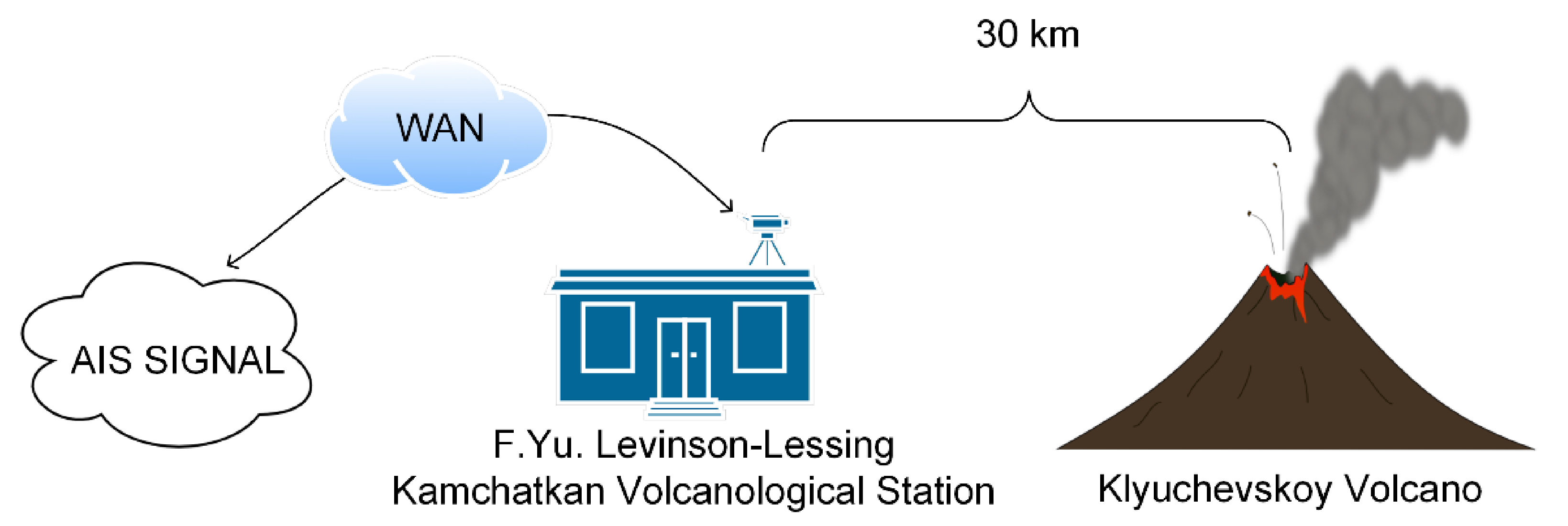
The considered video observation network capturing Kamchatka volcanoes consists of 9 cameras, installed on the Kamchatsky kray territory in two locations (
Table 1): in the village of Klyuchi in the F.Yu. Levinson-Lessing Kamchatkan volcanological station (cameras 1–5), and in the city of Petropavlovsk-Kamchatsky on the building of the Institute of Volcanology and Seismology of the Far Eastern Branch of the Russian Academy of Sciences (cameras 7–9). The processes of data collection, transmission and storage are controlled by the automated information system Signal [
21].
Each camera poll interval depends on the aviation colour code of the volcano set by the KVERT (Kamchatkan Volcanic Eruption Response Team) [
1] or is fixed due to individual observation mode and possible technical limitations. For this reason, the number of archive images for the same volcano in different years may be different.
In our study, we used the data archive, produced with camera 1 in 2017–2018, with a total image count of 871,110. This is a StarDot NetCam XL [
22] visible band camera, with Computar TV Zoom Lens [
23]. The camera watches the Klyuchevskoy volcano, with a distance to the crater of about 30 km. The main camera specification is summarized in
Table 2, and the conceptual dataflow described by
Figure 1.
This camera was chosen for study due to the stable operation of video and transmitting network equipment, as well as the fact that during the observation period from 2009 to present, numerous eruptions of the Klyuchevskoy volcano were documented. It is important for our study, since it allows us to use the results of studies of eruptions stored in KVERT VONA (Volcano Observatory Notice for Aviation) records, which were obtained, in particular, with remote sensing data processing in the VolSatView system.
2.2. Motivation
Real-time video observation network generates huge amounts of data. Up to 1440 images per day are sent to the archive by one camera of the network in Kamchatka, with 1 frame/min rate. At the same time, for a detailed analysis of the volcanic events (for example, to determine exact eruption times, plume velocity, etc.), the specified frame rate must be reduced by 5–10 times, which will certainly lead to a multiple increase in the volume of data generated. In the case of the active phase of the eruption, the operative analysis of such amount of data by volcanologists seems to be extremely difficult. It should be borne in mind that a certain part of the images does not contain valuable information, since the area of interest on them is hidden behind clouds, fog, bright sunlight or is not visible due to the night-time. In addition, during the eruption, the WAN link load also increases, due to the large volume of transmitted data, which, with limited telecommunication resources at observation points, also leads to errors in data transmission and to damaged images consequently. Considering the above problems, the task of filtering non-informative and damaged images is one of the key ones, the solution of which became possible with computer technologies.
Processing the ground-based cameras data with computer methods and technologies is successfully applied to detect and analyse volcano activity. In [
24] an automatic image processor based on the cellular neural networks is proposed to process analogical telecamera recordings. The accumulative difference image technique is adopted to provide real-time warning in case of volcanic activity events, with data framerate 0.05–0.1 s. The real-time thermo-graphic analysis of IR-camera data used to manage frame rate and automatically classify the volcano activity in [
13]. Computer vision methods and principal component analysis were used to determine lava flow trajectories for volcanoes of Ecuador in [
25]. In paper [
20], denoted to study of Villarrica volcano activity during February-April 2015, the BLOB detection algorithm is applied to each image in pre-selected region of interest, then a feature vector is extracted for detected BLOB. The artificial neural network of MLP-architecture was trained on manually labelled image dataset, providing five-class classification of image scenes.
The considered video observation network for Kamchatka volcanoes is equipped with visible band and VNIR band (IR-cut filter triggered at night-time) cameras, so thermographic data analysis methods cannot be applied. The minimal possible image frame rate is 1 min, due to limited link bandwidth at observation site. This does not allow us to successfully apply the algorithms for detecting volcanic activity based on dynamic characteristics. The sufficient framerate to detect relatively slow ash emissions is 1 frame per second, while 10–25 frames/s should be used for events with fast dynamic [
24]. The use of computer vision methods from [
25] for the volcanic events analysis requires a preselected image set with a clearly visible area of interest. In [
20], this is implemented on manually prepared dataset using histogram analysis of colour channels in a pre-selected region of interest. However, for the video observation network under consideration, there are situations when the camera lens moves (to observe events in a specific area of the volcano) or the zoom changes. The boundaries of the area of interest in the image change consequently (
Figure 2), so it is a problem to set them in advance and keep them up to date.
Considering the described peculiarities, we proposed to use methods based on the convolutional neural networks (CNN) as a tool for classifying images, which allows to analyse the whole frame, without highlighting the area of interest and preliminary feature vector extraction. With the help of a trained neural network, the continuous image stream can be automatically distributed over a given set of classes [
26,
27,
28], solving the problem of input control of data informativity. The most important condition for training a neural network is the presence of labelled image dataset. Considering the variety of scenes in the images of volcanoes, the training set size should be large enough, and the set itself should include images taken in various weather and seasonal conditions. Given the huge size of the unstructured archive available (see
Table 1), it is time consuming to create such a dataset manually. There are no publicly available labelled datasets of volcanoes. In this regard, we divided the solution of the volcano images classification problem into two interrelated parts—the development of algorithms to create a marked observational data set and consecutive training the neural network for classifying images.
3. Methods and Algorithms for Volcano Image Analysis and the Results of Their Approbation
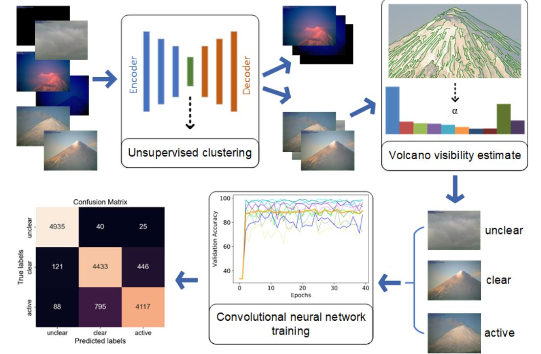
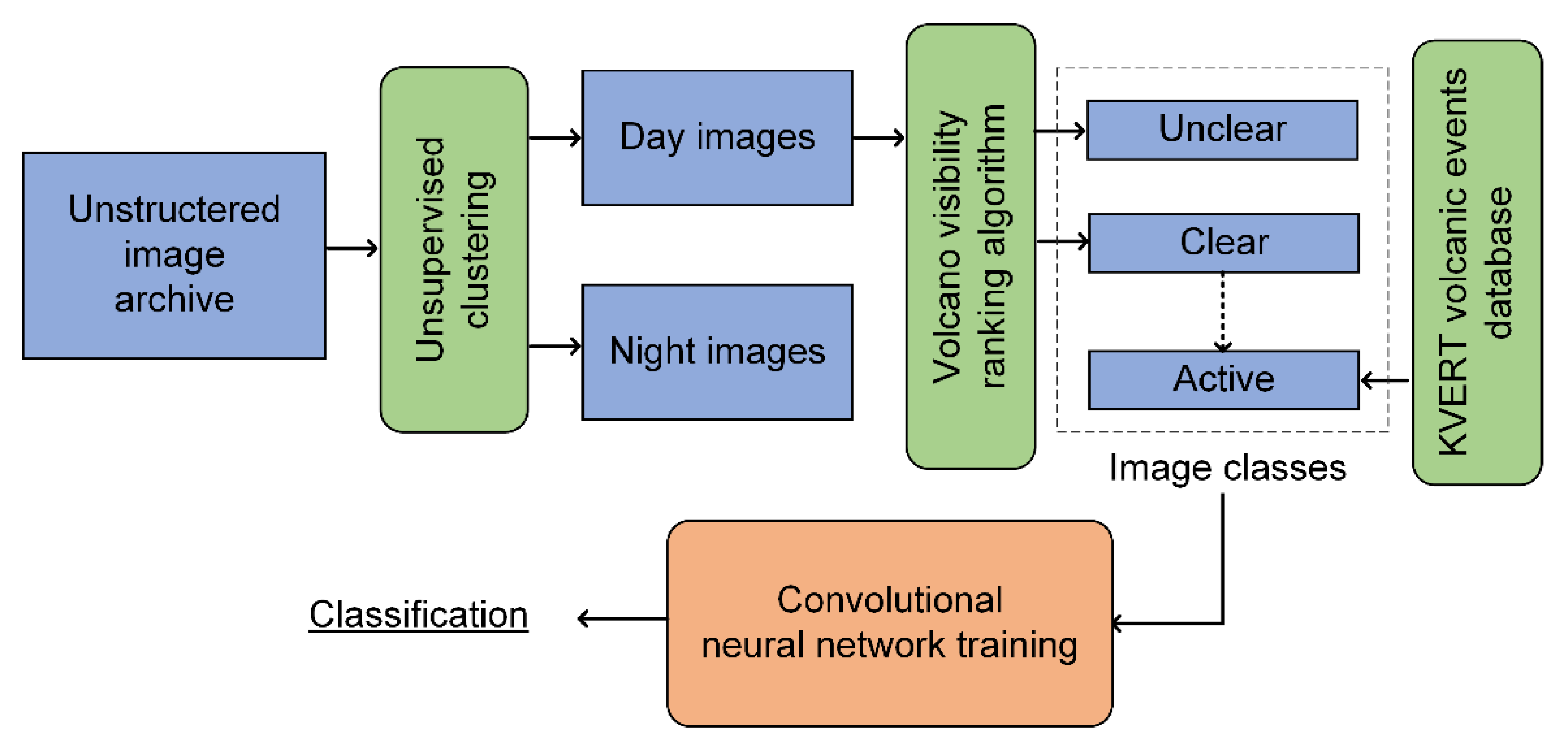
To create and adopt a labelled volcano image dataset from the unstructured archive we propose a multistage approach, including the use of author‘s methods adapted to the task (
Figure 3).
The source image archive is divided into daytime and night-time image sets with the unsupervised clustering approach.
For daytime images, the visibility of the volcano on the image is assessed, which makes it possible to rank the images according to the degree of their potential informativeness.
Based on the joint analysis of the estimates obtained for the images and data from the KVERT reports on the activity of Klyuchevskoy volcano, a class-labelled dataset is assembled.
The created image dataset is used to train and test the convolutional neural network.
Figure 3.
The flowchart diagram of the proposed algorithm to produce labelled dataset for CNN classification training.
Figure 3.
The flowchart diagram of the proposed algorithm to produce labelled dataset for CNN classification training.
Below is the detailed description of the proposed methods and algorithms.
3.1. Day/Night Image Clustering
The considered video camera has no IR-cut filter, therefore images generated by that camera at night-time contain no useful information due to very low illumination. So those images should be determined and filtered. The simplest approach could be to calculate times of different twilight types (civil dawn (sunset begin), sunset end, sunrise begin, civil dusk (sunrise end), etc.) at given geographical point using the sunrise equation [
29], and then to compare those times with the image timestamp. However, it was found that this approach doesn’t give stable criteria to consider image scene as night, because sometimes actual illumination remains enough to produce informative images for some period after sunset end (or some period before sunrise begin). In addition, sometimes the correct image timestamp is not available due to camera time synchronization errors. So, it is better to rely on the image itself. An image analysis approach is proposed in [
30], applying a histogram statistics thresholding in HSV colour space to detect day and night scenes. It was improved in [
31], resulting in scene classification precision of 96%. However, this method requires proper threshold parameters selection to meet considered image semantics.
Our approach is to adopt an unsupervised clustering, provided by DCEC architecture from paper [
32]. It proposes a special clustering layer attached to embedding layer of convolutional autoencoder neural network. In the pretraining phase, latent features are extracted from input data, and autoencoder network weights adjusted to reconstruct input images using MSE loss function. Then a given number of clusters are initialized with k-means for features extracted, and further training updates feature clustering distribution, using Kullback-Leibler divergence as a loss function. The resulting neural network weights could be used to split input dataset into a given number of clusters. In [
32], authors use DCEC to clusterize MNIST dataset consisting of 70,000 handwritten digits of size 28 × 28.
To train the DCEC model, we used Klyuchevskoy volcano archive for 2018 (351,318 images) as an input dataset. Because archive temporal resolution is 1 min, the adjacent images have minimal difference in day/night semantics, so only every third archive item was used for pretraining, resulting in a dataset of 117,106 images. Input images were resized to 256 × 256 and normalized. Pretraining was performed for 300 epochs with a batch size of 256. Label divergence has achieved 0.01 tolerance at the first train epoch. The trained model was tested over the 2018 archive. The results of clustering were verified, where possible, with sunrise equation output. The civil dusk and civil dawn times were used as approximate thresholds to consider image scene day or night. All the cases, where clustering result differs from verification, were checked manually.
Figure 4 shows how clustering results differ from sunset and sunrise time periods and gives a more accurate day/night image dataset split. The only 266 of total 351,318 images (0.07%) were clustered incorrectly (
Figure 5).
3.2. Parametric Methods for Volcano Visibility Estimate
A large number of day images are unusable for further analysis because the region of interest is obscured by clouds, fog, bright sunlight artifacts, etc. For preliminary quality ranking of images, we developed an algorithm, which estimates volcano visibility on the image. The basic idea is to represent volcano contours as polylines, with branching in vertexes. Defined by a set of parameters, these polylines are called volcano parametric contours. Comparing parametric contours for image with parametric contours for the preselected reference image, we can estimate the visibility of the observed object.
If compared contours are extracted with edge detection algorithm, then the distance between edge pixels on different images is measured. This distance could be the same for several pixels relative to some reference pixels, which gives false response in contours intersection areas and leads to multiple comparisons of one contour of the image with different contours of another image. With parametric contours, we analyse how one polyline falls on another polyline in shape, while all the segments of this polyline may not coincide at all, especially if they are small. The average distance between the two polylines plays the main role. This allows us to handle the camera possible shifts.
3.2.1. Parametric Contours Building
Parametric contouring building begins with a discrete edges map, extracted using the Canny edge detector [
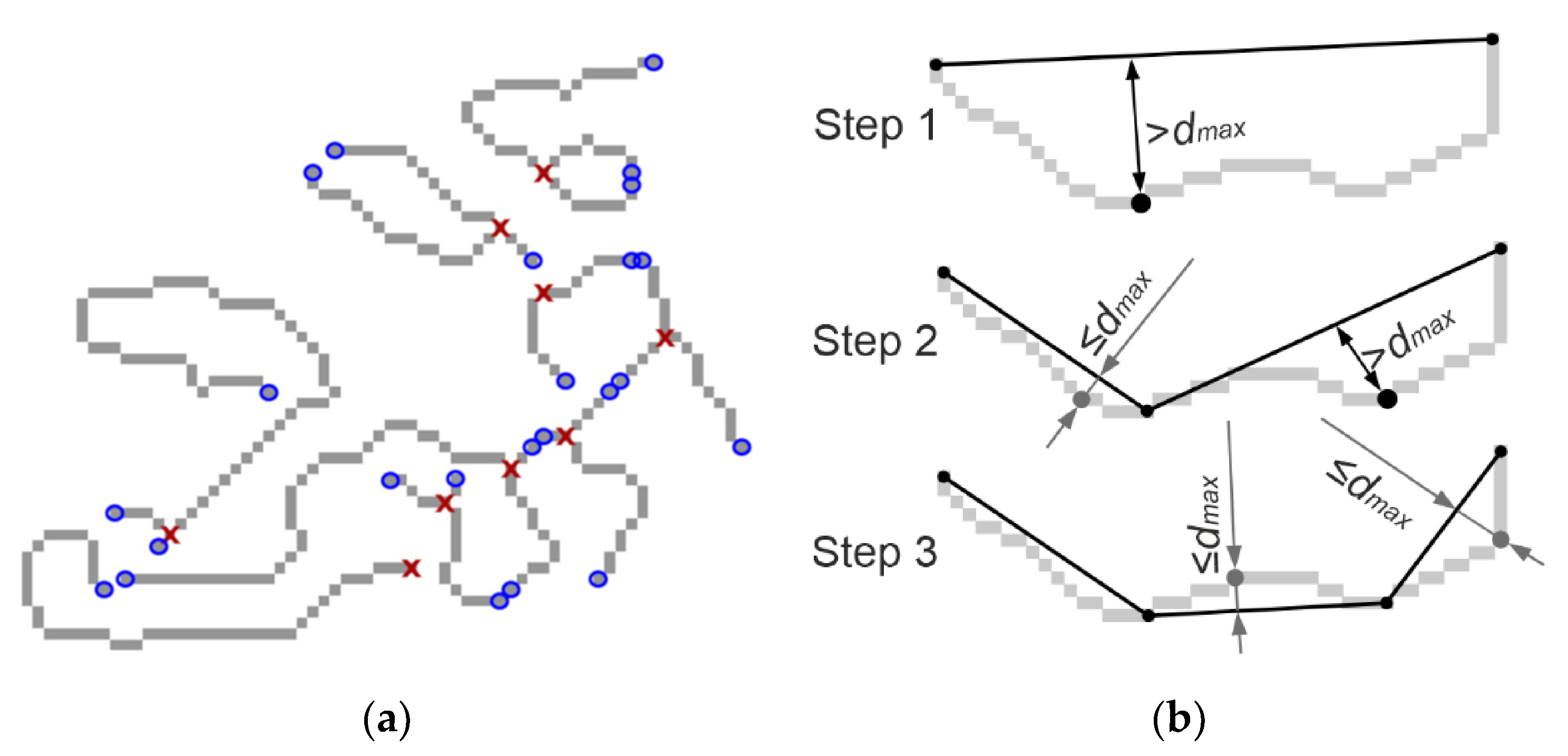
33]. Then, on the map, the sequences of pixels are selected between the branch points and the ends of the paths (
Figure 6a). After that, the obtained pixel chains are used to construct polylines, by recursively dividing the chains into straight lines connecting the starting and ending pixels. The split point is selected in the pixel, the distance from which to the line is maximum, if this distance exceeds the
threshold. An example of constructing a polyline along a chain of pixels is shown in
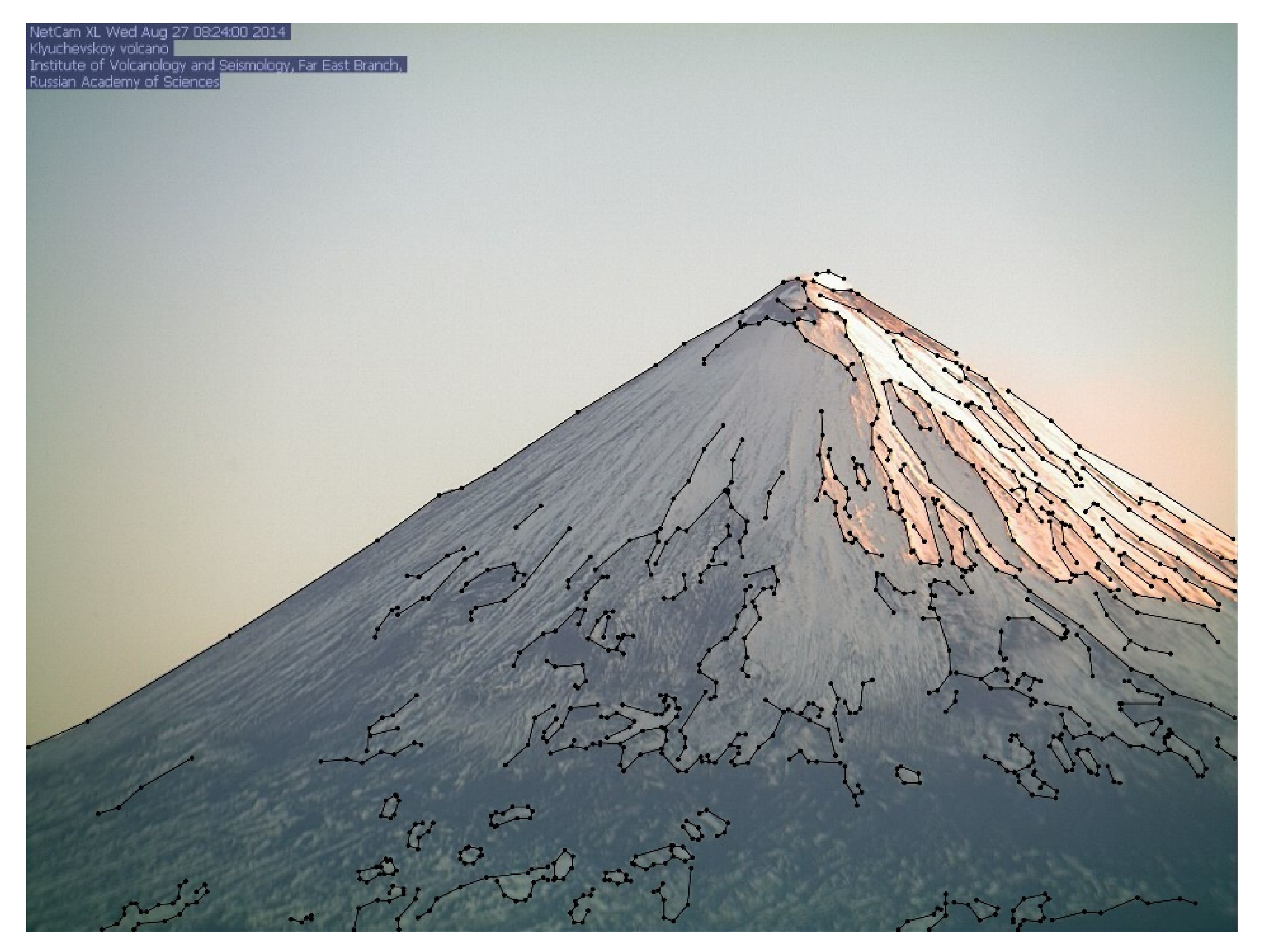
Figure 6b. Result of constructing parametric contours is shown in
Figure 7.
The procedure for comparing parametric contours obtained for two images is described in [
34]. The result of the comparison is expressed by the estimate
:
—set of numbers of compared polylines,
—the number of compared segment pairs for polyline ,
and —set of segments for first and second image respectively,
—compared segments,
—segments of the second image,
—common part length of segments and ,
—length of segment .
This estimate shows the occurrence of the contours of the first image in the second (reference) image, which is equal to the ratio of the total length of the matched contours to the total length of the contours in the second image.
3.2.2. Finding the Shift between Contours
Due to the impact on the camera of environmental factors (wind load, temperature variations, etc.), as well as due to small manual turns of the camera to change the observation area, the contours in different images may have an offset relative to each other. The study of the image archive showed that the relative shift between the contours can reach 10% of the image width. Therefore, to align the parametric contours relative to each other, it is proposed to use the shift calculated using the discrete edges map. The use of the vector makes it possible to compensate for relative displacements of more than 20% of the image width.
Let the images received from the camera have dimensions
pixels, then each pixel of this image has the number
, where
,
—coordinates of the pixel in the image. Using the Canny edge pixel detection algorithm for the image under study, we calculate the set
, consisting of the numbers of the edge points. The difference score between two sets of edge pixels numbers
and
, obtained for two images, is calculated as:
where
is the distance between pixels with numbers
and
, and
is a maximum distance between pixels which could be compared. The search for the minimum distance in (1) is carried out using the distance map to the edge points
.
To align the parametric contours, consider the shifted edges points set
where
,
,
. Using this set, we find the shift as:
Shift calculation in (2) is carried out on the image reduced by times, where , and with . When shift for reduced image is found, the shift for the original-size image is calculated with gradient descent method, starting from pint , . The function may not have one clear minimum, therefore, to initialize the gradient descent method, it is necessary to take up to 5 minimums, which are worse than the global minimum by no more than 20%.
3.2.3. Building Reference Contours
To assess the volcano visibility on the image, the parametric contours extracted for it are compared with some reference contours, which are constructed for preselected images taken in good weather conditions with good illumination and at different seasons. Such images are called reference images, their number was determined during our experiments.
For reference image
i,
, we find
and calculate
,
. The shift is found as:
The parametric contours of reference image
i are found as described in
Section 3.2.1 and then shifted by
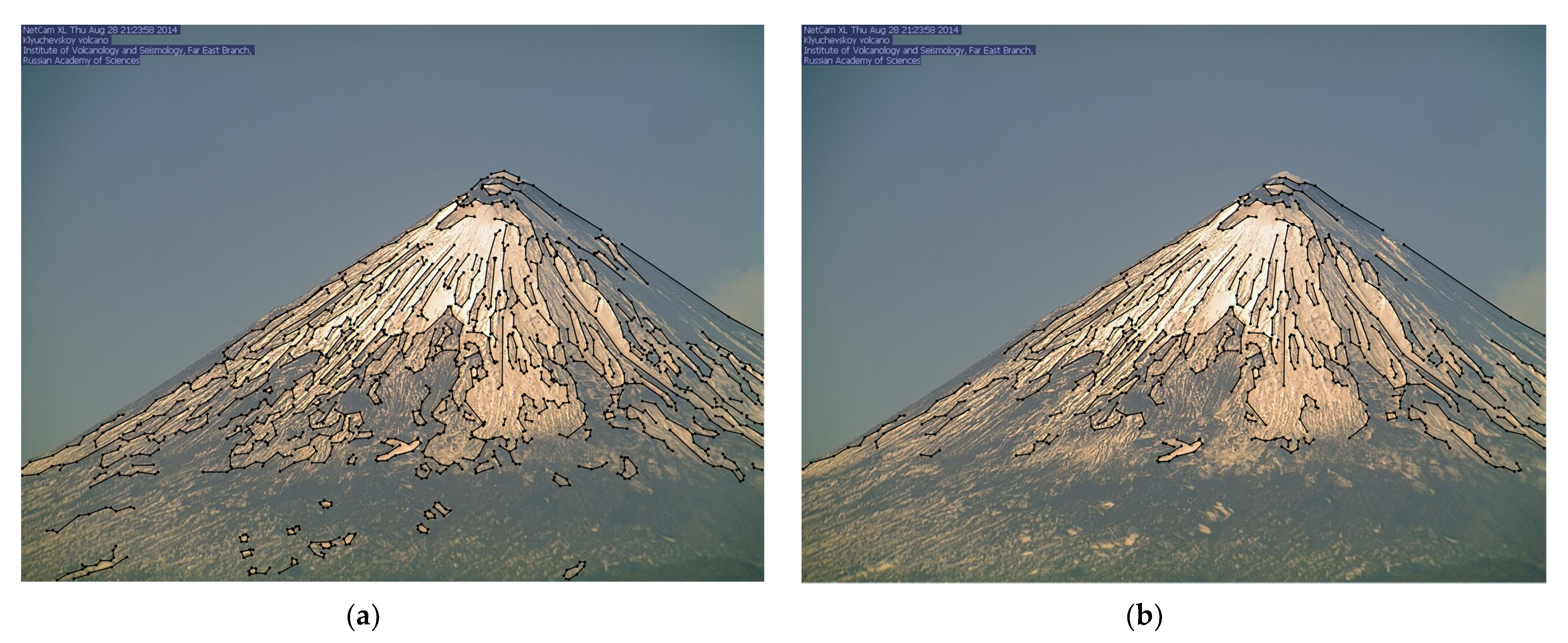
. The contours for all reference images are compared in pairs, and those contours that occur in at least
images, are selected as reference ones. The
is selected in the range from 0.5 to 1.0, it allows to control the contribution of the most characteristic contours of the considered volcano to obtain the most accurate estimates for the studied images (
Figure 8).
The extracted reference contours are divided into internal and external ones. The external contours are composed of line segments that have a maximum y-coordinate for point of intersection with vertical lines drawn with one pixel distance. The rest of the contours are considered internal. This separation allows us to correctly analyse images taken, for example, in conditions of sunlight, when only the general outline of the volcano is visible. In this case, analysis on a common set of contours will result in an underestimated visibility, while the outer contours of the volcano will be fully visible.
The visibility estimate contours for the tested image is calculated by the formula:
where
and
—the occurrence of external and internal reference contours on the tested image, respectively, a
and
—the occurrence of external and internal reference contours in the reference image
i.
3.2.4. Image Frequency Characteristic Estimate
Partial clouds in the frame can affect the contour visibility estimates in different ways. For example, it can be overestimated due to the partial coincidence of the cloud contours with the reference contours or underestimated when the lower part of the frame is hidden behind the clouds, but at the same time the upper part of the volcano with a potential region of interest is visible. To take this effect into account, we additionally estimated the contribution of the frequencies involved in the formation of the image.
Let us denote the image brightness component as
,
,
, where
w и
h are image width and height respectively. To determine which frequencies are involved in the formation of
, and what contribution they make, we divide the frequency spectrum into octaves. It is most convenient to do this if the width and height of the image are powers of two:
,
,
. Since the considered images have a size of 1024 × 768, they were scaled to 1024 × 1024, and
. The contribution vector
of each octave to the formation of the image is called the vector of the contribution of frequencies or the frequency characteristic of the image. The vector
,
, is calculated using the following formulas:
Like in the approach for contours, the frequency characteristics of the analysed images are compared with the reference characteristic
calculated for the reference images:
where
—
i-th reference image,
—frequency characteristic of
i-th reference image. To compare the frequency characteristics
with the reference
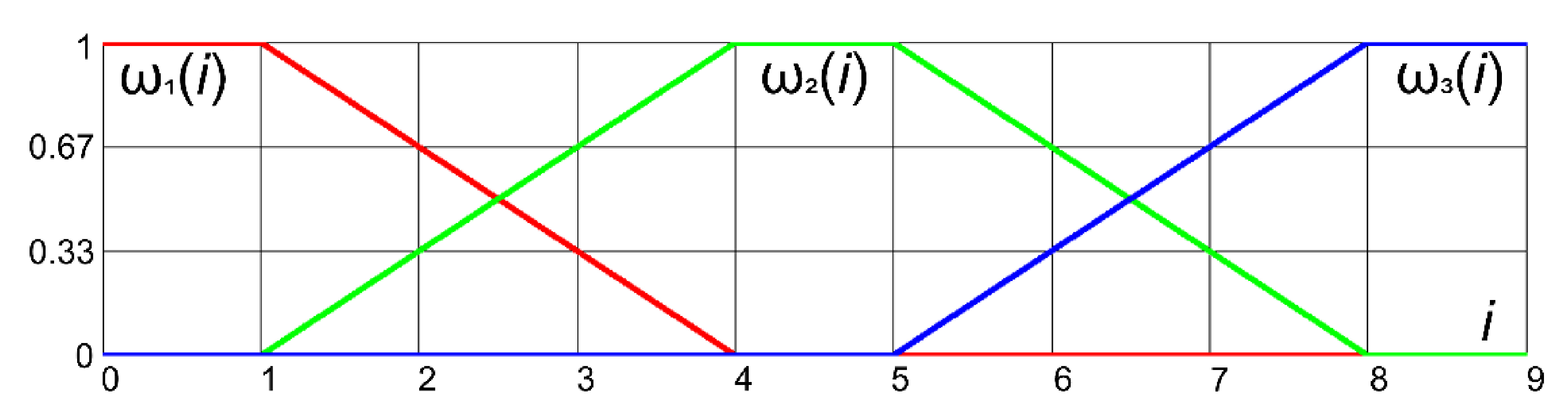
, the following estimate is used:
where
are base function, which determines the influence of the parameters
on individual groups of frequencies (
Figure 9),
and
,
are constant parameters that are calculated experimentally. To find them, we choose
images with different scenes, and manually define for them a range of estimates: [
], where
—frequency characteristics of
l-th image,
. The values of
and
are determined by solving the following minimization problem:
where
is a distance function, defined as:
Values of
and
are constant for each camera.
Table 3 contains the parameters values for considered camera.
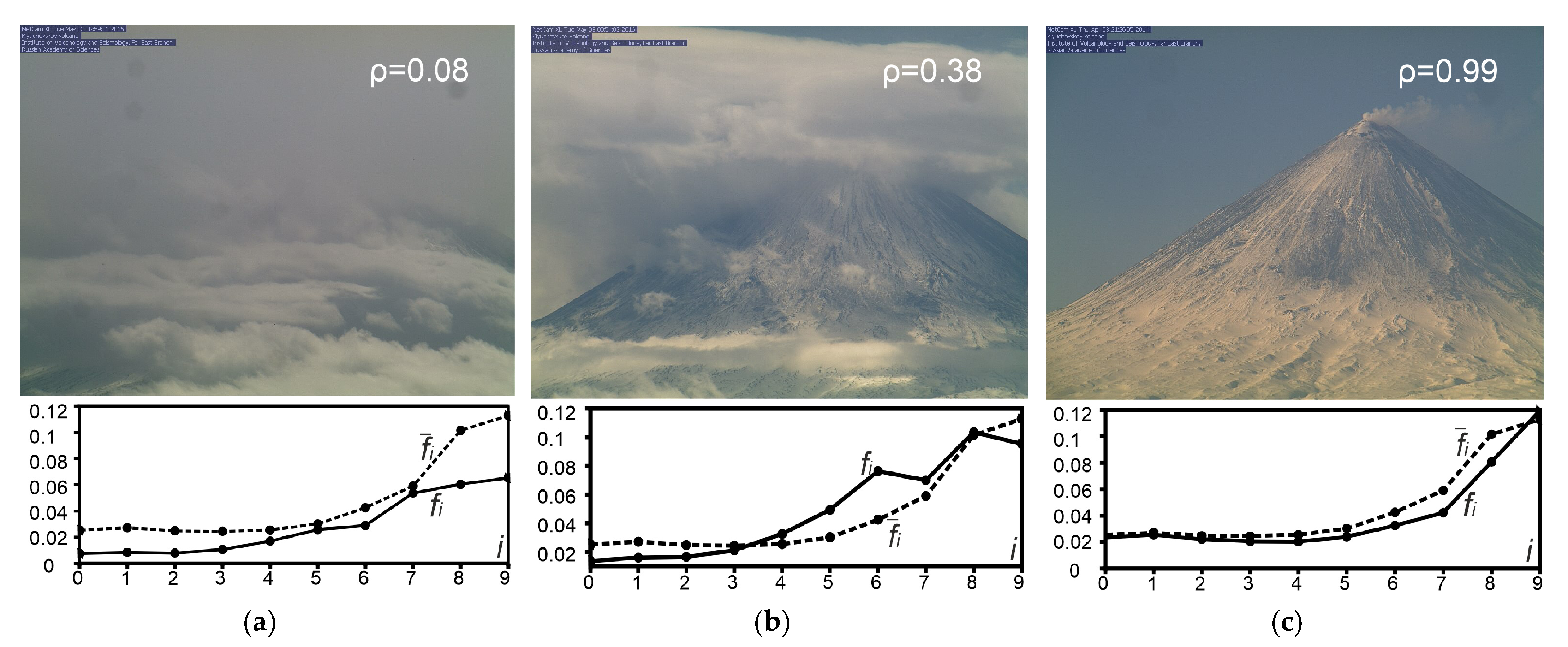
The
Figure 10 shows the different Klyuchevskoy volcano scenes with their corresponding
-estimates and frequency characteristics comparing to reference ones, calculated by Equations (3)–(6).
The result volcano visibility score
for the image is determined as follows:
Contours visibility estimate makes the main contribution to . If is in the -vicinity of defined threshold , then frequency characteristics -estimate is used for result score correction.
3.3. Emerging the Labelled Dataset and CNN Training
The proposed algorithms, described in
Section 3.1 and
Section 3.2, were applied to the Klyuchevskoy volcano image archive for 2017, which includes 519,792 items. At the first stage, the defective images, generated in poor transmission network conditions, were filtered, by checking the last two bytes of each image, which should be equal to ‘0xff0xd9′ for correct JPEG-images. At the second stage, the inference of trained DCEC model from
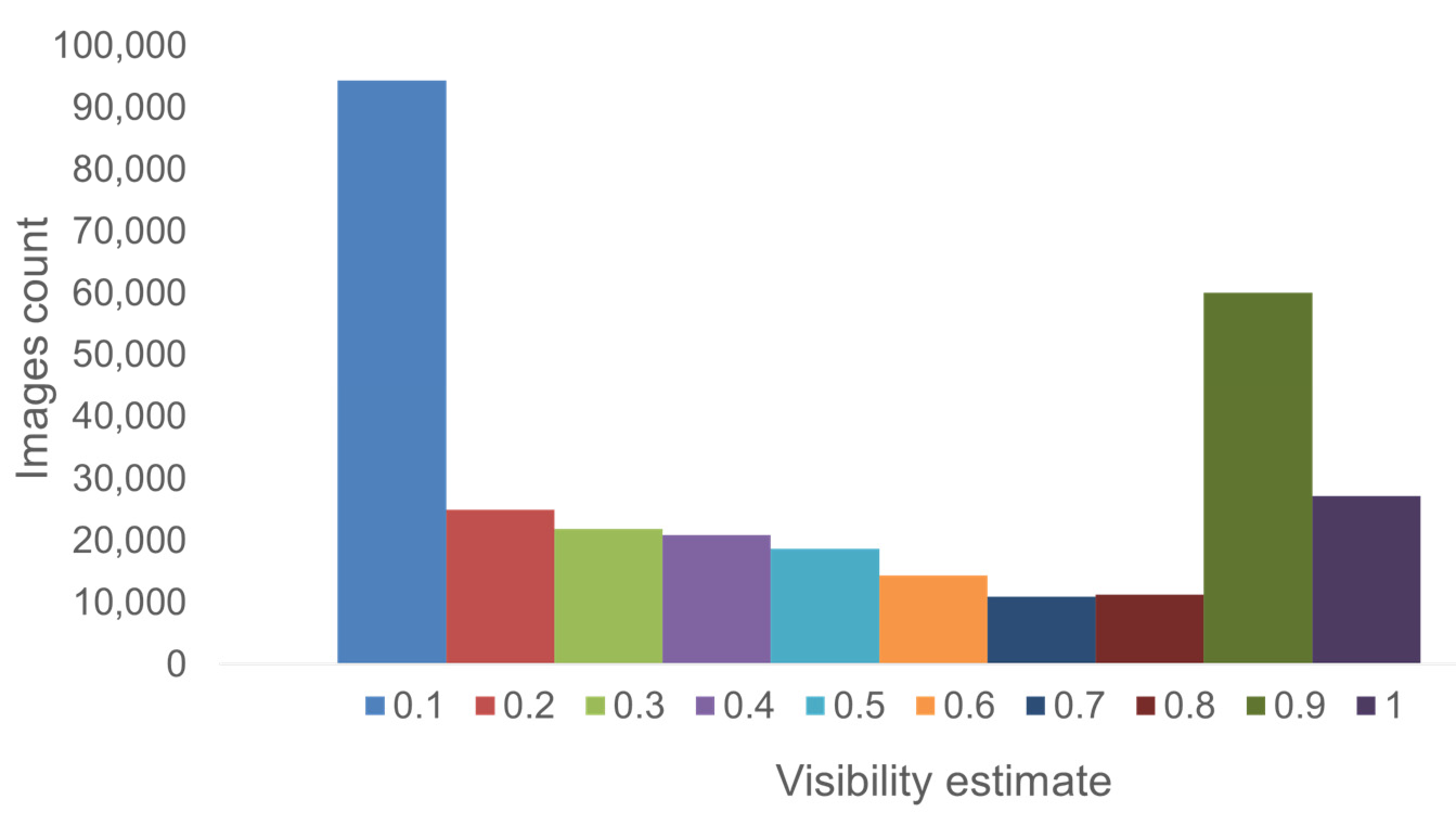
Section 3.1, was carried out, dividing archive in two clusters: 302,520 of day and 217,272 of night images. Next, the visibility estimation algorithm was applied to the day cluster.
Figure 11 shows the distribution of images by calculated visibility estimate
.
The proposed visibility ranking approach allows to sort thousands of images by their potential usability. This made it possible to create a labelled dataset for future CNN training.
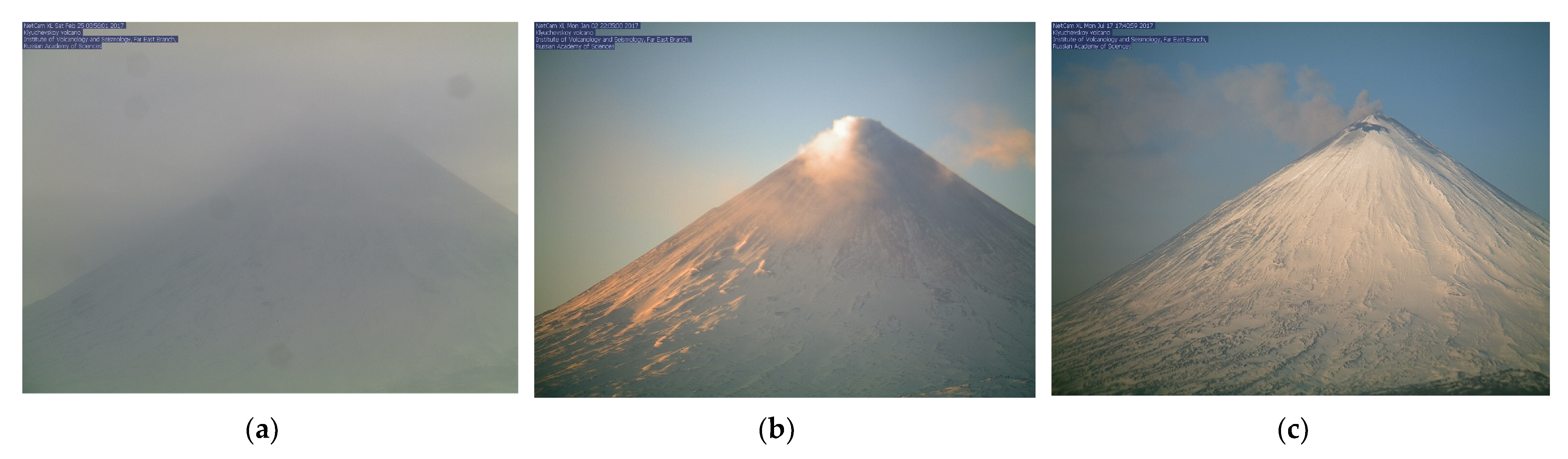
For day images, we define the next three classes, which describes the most distinctive and important states:
unclear—region of interest is not visible because of clouds, different sunlight effects, etc.
clear—good visibility, no significant volcanic activity.
active—good visibility, volcano activity detected.
To assemble the dataset, labelled with defined classes, we completed the following steps.
The total dataset size is 15,000 images, with an equal number of images for each class to make it balanced.
There are different state-of-art deep CNN architectures for feature extraction and image classification: ResNet [
36], DenseNet [
37], EfficientNet [
38]. The last one has the smallest memory footprint and performs faster [
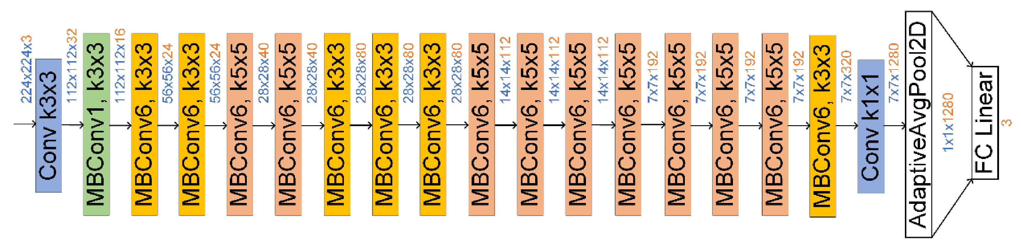
38], so we adopted an EfficientNet-B0 architecture for volcano images classification. It consists of input convolutional layer with 3-channel input with size 224 × 244, followed by sequence of Mobile Inverted Residual Bottleneck Blocks [
38] for feature maps extraction (
Figure 12). The final convolution layer is the adaptive 2d pooling followed by a fully connected layer of size 3, by number of predicted classes.
We conduct model training from scratch and didn’t use any pretrained model weights (i.e., on ImageNet database [
39]). The Nvidia Tesla P100 GPU was used for calculations. No special input data augmentation was applied, except a resize to 224 × 224 and normalization. Instead of standard ImageNet per-channel mean and std values, the following values were calculated for our dataset:
The 10-fold cross-validation was applied to dataset, with the StratifiedKFold from Scikit-learn package [
40]. This preserves class balance in different folds. The model was trained and validated 10 times with the following hyperparameters:
number of epochs—40;
batch size—64;
learning rate—0.001.
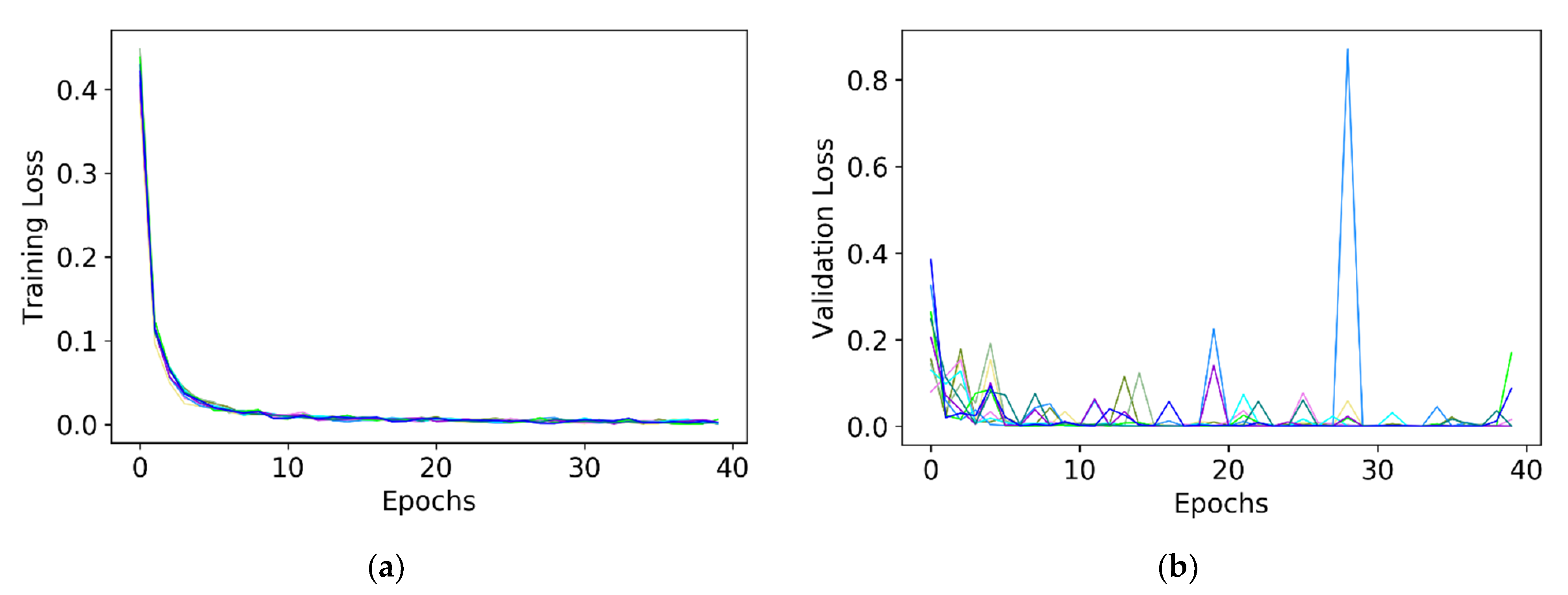
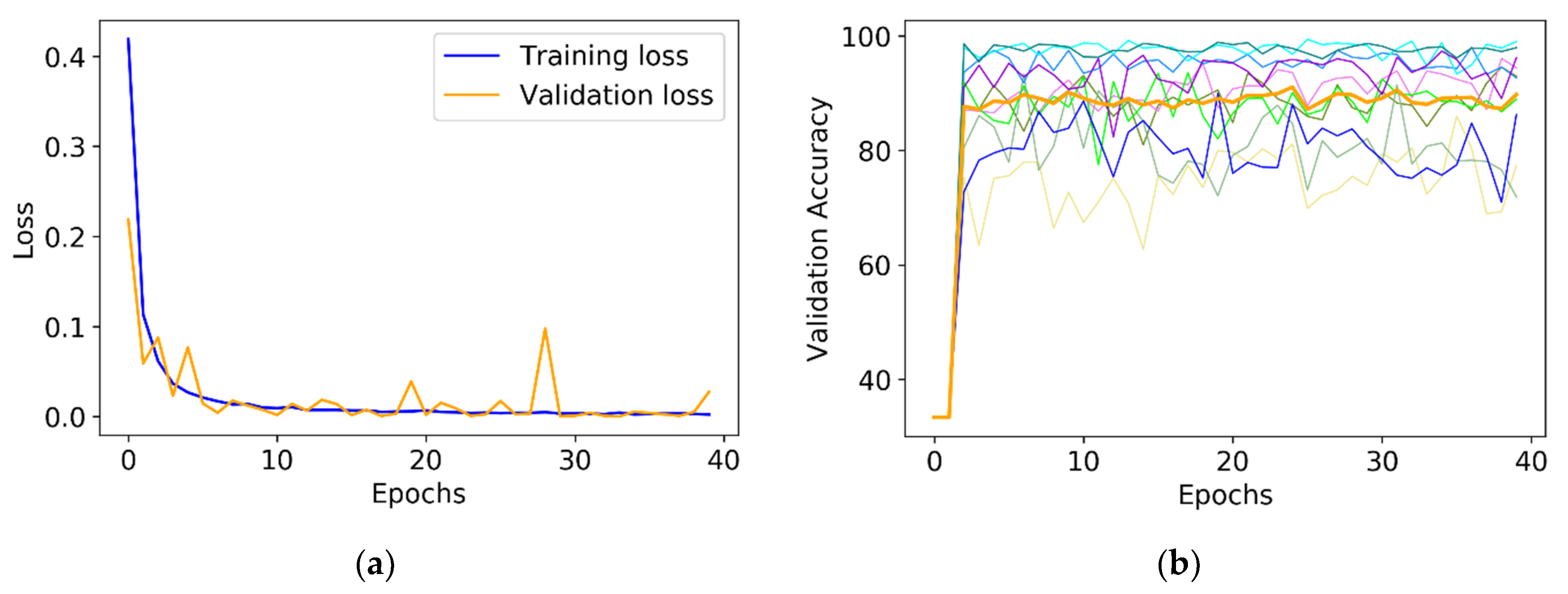
Figure 13 shows training and validation loss by epoch for each cross-validation fold.
The metric averaged by cross-validation folds are shown on
Figure 14. The best average accuracy of 91% with a standard deviation of 5.28 is achieved at 24 epoch.
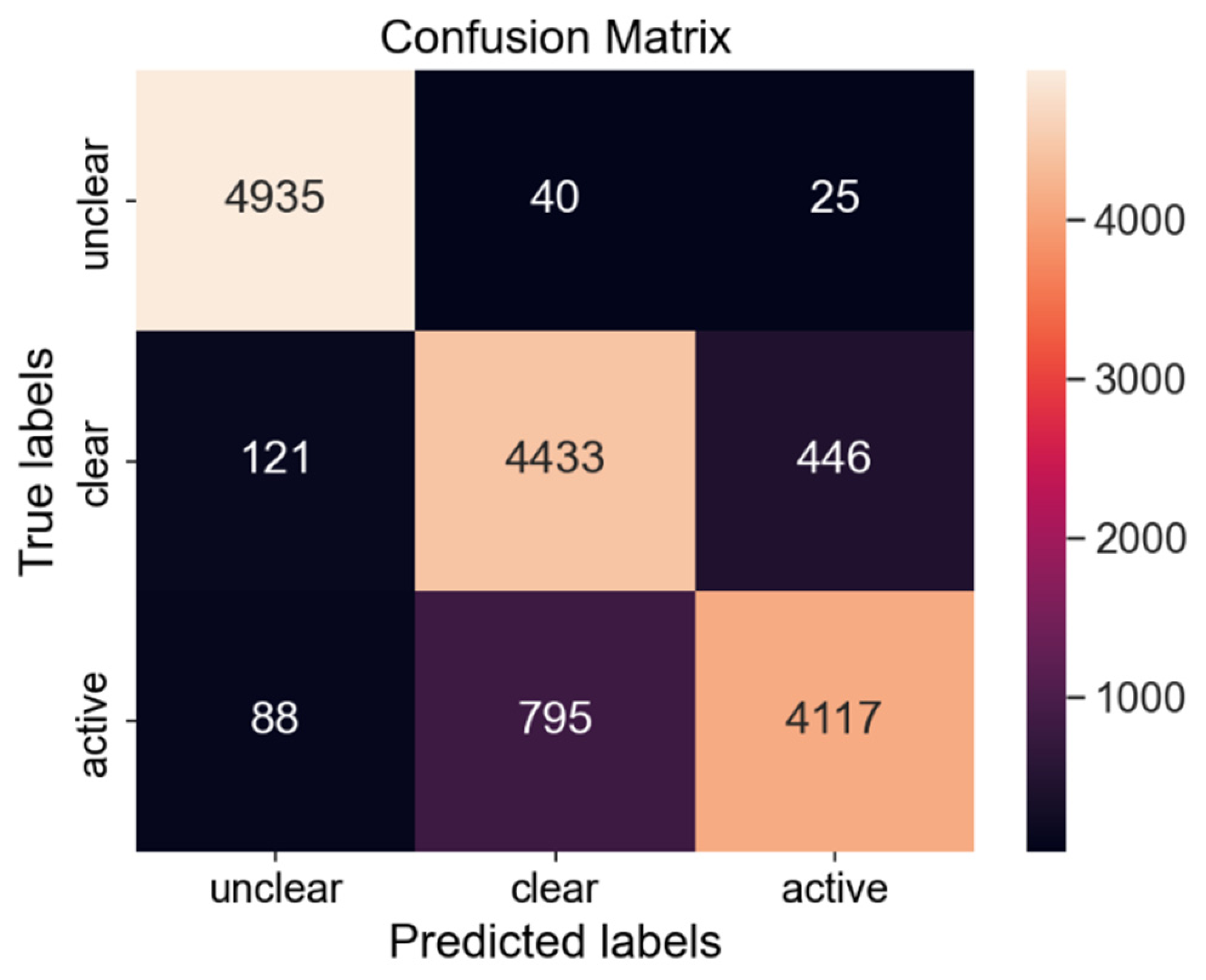
The confusion matrix overall folds presented on
Figure 15. The model predicts ‘unclear’ class better, while the ‘active’ class the most difficult to predict correctly.
Figure 16 shows examples of correctly classified images.
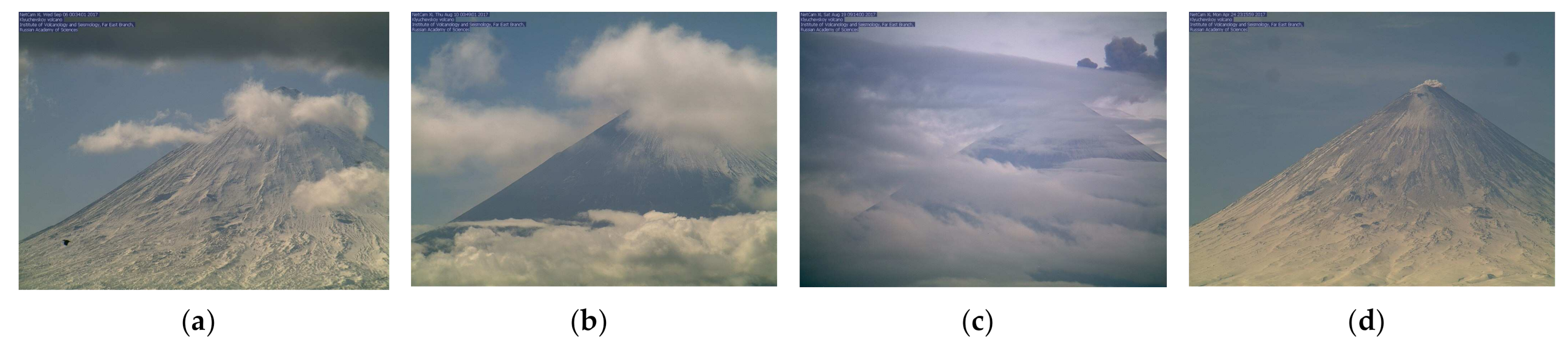
The big variety of scenes with clouds leads to incorrect classifications for some images.
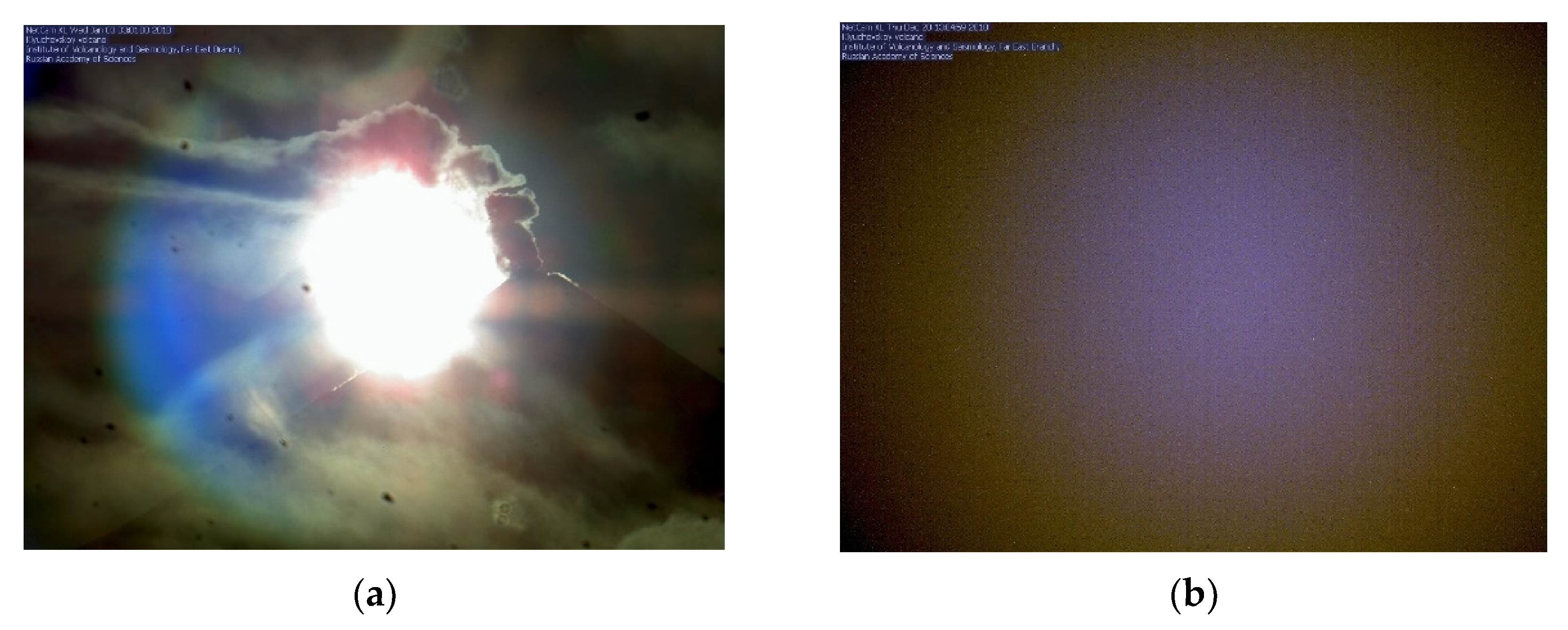
Figure 17 shows examples of misclassification:
(a)—image marked as ‘unclear’, while actual volcano rim visibility allows to observe possible activity.
(b)—image, false labelled as ‘active’ due to cloud cover.
(c)—the scene marked as ‘unclear’, but ash plume is visible behind the scattered clouds.
(d)—actual light emission on image classified as clear because light emission is almost masked by the volcano itself.
Figure 17.
Examples of incorrectly classified scenes of Klyuchevskoy volcano: (a) image with true label ‘clear’ classified as ‘unclear’; (b) image with true label ‘unclear’ classified as ‘active’; (c) image with true label ‘active’ classified as ‘unclear’; (d) image with true label ‘active’ classified as ‘clear’.
4. Discussion
Analysing the results of the conducted study, we conclude that the unsupervised clustering is an approach to determine day and night images, which is possibly applicable for any visible band camera. We conducted experiments on inference the DCEC model which was trained on the Klyuchevskoy volcano image archive, with data archive for 2018 of the camera capturing the Sheveluch volcano, and received good results for day/night clusters. This is achieved by sufficient size of the training set, so when model extracts feature maps from many images and adjusts weights to cluster embedded features into two classes, it finally ignores any object edges semantics, focusing on general illumination semantics. For cameras considered in this paper with frame rate 1/60 s we assembled training dataset from a one-year archive, taking every third image. This rule, perhaps, should be expanded for any other camera with higher frame rate (i.e., take every 10th image, for example), or reduced for lower frame rate, using all archive for DCEC model training.
The developed algorithms for volcano visibility estimate in the image cannot be used for a full analysis of volcanic events, since they only consider the visibility of the observed object. However, having this image ranking approach, we exclude a big amount of uninformative data from further analysis. This makes it possible to efficiently work with observation data.
The EfficientNet convolutional neural network trained on labelled dataset shows the average accuracy of 91% in classification daytime images. A distinctive feature of our proposed solution is that the image classification as well as detection of images with possible volcano activity is carried out without specifying the region of interest, like it is done in paper [
20]. This makes it possible to use them for an automated classification of images continuously received from the observation network under the conditions when camera lens position is changed. At the same time, our approach does not extract specific signs of volcanic activity, like lava flows [
25], but allows to categorize image itself, filtering out the images with no valuable information and detecting images with possible volcano activity, which can further be analysed in detail. At the same time, due to the distinctive features of the relief of Klyuchevskoy volcano, the neural network trained on its images will show a lower classification accuracy (in ‘clear’ and ‘active’ classes) for images of volcanoes, whose visual contour differs significantly (i.e., Sheveluch volcano). This may require assembling the additional dataset with the implemented ranking algorithm, and the subsequent CNN training using the transfer learning methods.
The obtained results show the efficiency of convolutional neural networks application to problems of classification of volcano images. An analysis of cases with misclassified images suggests the next promising study direction—semantic segmentation of ash and steam-gas emissions using neural networks, for example, based on the Mask-RCNN or UNet architecture. This will allow to detect signs of volcanic activity in conditions, where image region of interest is partially obscured by clouds or other phenomena. With emission segmented on image, it is also possible to analyse volcanic events in more detail. However, assembling the labelled dataset for training these kinds of neural networks is an even more time-consuming task and will be a subject of our future research.


