Abstract
From network RTK to PPP-RTK, it is highly expected that high-precision positioning within a few minutes can be achieved with a sparse reference network. In this study, we investigate a rapid multi-frequency PPP convergence strategy based on Galileo E1/E5a/E6 and BeiDou-3 B1C/B2a/B3I signals, whose unambiguous wide-lane observables can efficiently assist in speeding up narrow-lane ambiguity resolution. Furthermore, frequency-specific biases existing on the third-frequency observables have been observed to slow down multi-frequency PPP-AR convergence. In this study, we partially mitigated their effects by estimating a second satellite clock for the third frequency of signals. We validated this approach with one month of data collected from 22 stations. On average, it took about 18 min for PPP wide-lane ambiguity resolution (PPP-WAR) to converge, while 32 min were required for ambiguity-float PPP. Compared with dual-frequency PPP-AR, which needed nearly 12 min to converge, multi-frequency PPP-AR required 6 min only. Once there were more than 10 satellites involved in PPP, the convergence could be achieved within 3 min on average. Meanwhile, 81% and 62% of multi-frequency PPP-AR solutions converged successfully within 5 and 1 min, respectively. Finally, we carried out a vehicle-borne experiment to validate this approach in a kinematic environment. Owing to frequent cycle slips during the movement of vehicle, it took 14 min for B1C/B2a/B3I and E1/E5a/E6 PPP-AR to obtain reliable positions, and 19 min for those using the other signal combinations B1C/B2a/B2b and E1/E5a/E5b, owning to higher noise. Overall, these results are promising for achieving high-precision PPP positioning globally within a few minutes if multi-frequency biases can be handled well in the data processing.
1. Introduction
Precise point positioning (PPP) can achieve centimeter-level absolute positioning without any nearby reference stations [1,2]. However, PPP has long been plagued by its slow convergences, spanning a few tens of minutes, to ambiguity-fixed solutions, which hinders its application in some time-critical scenarios such as autonomous driving [3,4]. Ref. [5] demonstrated that real-time kinematic (RTK) positioning could converge to the comparable precision of PPP within a few seconds on a short baseline (≤10 km). However, the requirement of a dense reference network makes it difficult to apply RTK to wide areas. PPP using RTK corrections (i.e., PPP-RTK) was developed since 2005, which was claimed to achieve single receiver fast convergence or re-convergence [6,7]. Similarly, ref. [8] also stated that such a dense local reference network was always required to calculate precise corrections for rapid centimeter-level positioning.
With the rapid development of BeiDou and Galileo towards their full-operation constellations [9], there are more than 100 global navigation satellite system (GNSS) satellites in space. The integration of all GNSSs, rather than only the Global Satellite System (GPS), can provide better satellite geometry and improves the performance of rapid PPP ambiguity resolution (PPP-AR). Ref. [10] carried out PPP-AR using GPS and GLONASS data and claimed that 50% of solutions could converge in 5 min, while this rate was only 4% for GPS-only case. Ref. [11] implemented GPS/GLONASS/BeiDou-2 PPP-AR using a regional network. They demonstrated that 90% of multi-GNSS solutions could be initialized successfully within 10 min while only 16% for GPS-only PPP.
Other than multiple constellations, multi-frequency GNSS signals have brought new opportunities for rapid PPP convergences. Particularly, more than three signal frequencies are transmitted by GPS, BeiDou-2/3, Galileo, and QZSS (Quasi-Zenith Satellite System) satellites, which facilitates the formation of combination observables with favorable long wavelengths and low noise. Ref. [12] envisioned a geometry-free combination observable using triple-frequency GPS signals for rapid double-difference ambiguity resolution. For PPP, ref. [13] formulated an ionosphere-free phase observable, which was based on ambiguity-fixed wide-lane (L1–L2) and extra-wide-lane (L2–L5) observables [14,15]. They stated that this observable could be used to speed up PPP-AR, though its carrier-phase noise was amplified by over 100 times. They used simulated GPS L1/L2/L5 data and achieved PPP-AR within 65 s for 99% solutions. Later, they developed an approach using an uncombined PPP model to process real multi-frequency signals. Their experiments showed that the mean convergence times of GPS/Galileo/BeiDou-2/QZSS (L1/L2/L5, E1/E5a/E5b, B1/B2/B3 and L1/L2/L5) PPP-AR was shortened from 9 to 6 min compared with dual-frequency PPP-AR [16]. Using multi-frequency Galileo and BDS data, ref. [17] demonstrated that the positioning precision could be improved by over 30% on average after resolving ambiguities. Ref. [18] stated that by resolving Galileo (E1/E5a/E5b) extra-wide- and wide-lane ambiguities, the time required for narrow-lane ambiguity fixing could be decreased by 20%. Similarly, ref. [19] implemented multi-frequency GPS/Galileo/BeiDou-2 (L1/L2/L5, E1/E5a/E5b/E6 and B1/B2/B3) PPP-AR and reached 5 min of convergence time on average. However, one drawback of the multi-frequency combinations above is that the combined observable noise is over 100 times that of raw carrier-phase observation.
On account of the five signal frequencies emitted by Galileo and BeiDou satellites (i.e., E1/E5a/E5b/E5/E6 and B1C/B1I/B2a/B2b/B3I), favorable multi-frequency signal combinations whose noise is amplified by far less than 100 times, can be formed. Ref. [20] used a Galileo E1/E5a/E6 combination observable whose phase noise was amplified by only 67 times, and achieved instantaneous 20 cm point positioning accuracy in the horizontal components. Ref. [21] also demonstrated the positive effects of E1/E5a/E6 in PPP-AR from the perspective of frequency separation. They resolved multi-frequency raw ambiguities and achieved sub-decimeter convergence in 15 min at 90 percentiles. Ref. [22] demonstrated that BeiDou-3 B1C/B3I/B2a was another favorable combination that had comparable noise with that of Galileo E1/E5a/E6. They achieved single-epoch PPP wide-lane ambiguity resolution (PPP-WAR) based on E1/E5a/E6 and B1C/B3I/B2a signals in an urban environment. Therefore, it is promising that these two multi-frequency combination observables can be used to speed up narrow-lane ambiguity resolution as well. In this study, we implemented Galileo/BeiDou-3 triple-frequency PPP-AR with the E1/E5a/E6 and B1C/B3I/B2a signals, aiming at shortening PPP convergence times to a few minutes, preferably one minute.
2. Methods
In the following sections, we briefly derive the multi-frequency PPP function models based on undifferenced observables. The details about triple-frequency ambiguity resolution method in this study are displayed in the next section. Then the advantages of Galileo E1/E5a/E6 and BeiDou-3 B1C/B2a/B3I on achieving extremely fast PPP-AR are demonstrated.
2.1. Multi-Frequency PPP Model
GNSS multi-frequency original observations of pseudorange and carrier phase can be written as follows:
where and denote pseudorange and carrier phase observations of satellite on frequency ; is the geometry distance between satellite and station , which has absorbed troposphere delays; and represent receiver and satellite physical clock error in meters respectively; is the oblique-path ionosphere delay; whereas denotes corresponding frequency-dependent coefficients; we define and is the frequency on the band; marks the constellations. In this study, we define Galileo as “”, BeiDou as “”. and denote pseudorange hardware biases in meters of the receiver-pair and satellite-pair, respectively. Similarly, and are those in cycles of carrier-phase counterpart; is the wavelength of the band; denotes integer ambiguity, which is the unknown phase cycles when the receiver first tracks one signal; finally, and include the random noise of pseudorange and carrier phase observation, and unmodeled errors such as multipath.
Equation (1) cannot be solved directly owing to rank deficiency in a least-squares adjustment [23]. Reparameterization is required due to the correlation between clocks and hardware biases. Hardware biases and are usually lumped into clock parameters in the traditional dual-frequency PPP model; after the reparameterization, ionosphere-free pseudorange hardware biases are absorbed into clock parameters, while those of carrier-phase are absorbed into float ambiguity estimates. This strategy has been widely used in dual-frequency PPP data processing. However, it cannot be applied directly to multi-frequency data processing. In this study, the typical dual-frequency reparameterization above was applied to L1/L2, and we further estimated a receiver–satellite-dependent constant on each of the extra multi-frequency pseudoranges [16], that is
and
Taking triple-frequency data processing as an instance, the above parameters can be interpreted as
where , , , and represent the reparametrized receiver/satellite clocks, ionosphere delay, and float ambiguity. is the constant parameter estimated only on pseudorange observations beyond bands L1/L2. Differing from the integer ambiguity , is a float parameter because it has absorbed the combination of pseudorange and carrier-phase biases after reparameterization. In this study, we call these ambiguities with no integer nature as float ambiguities. Equation (2) is suitable for satellites that are free from time-varying inter-frequency clock biases (IFCBs). For satellites that suffer from IFCBs, we can estimate a second satellite clock on the third frequency or other extra frequencies [24], that is
and in the triple-frequency case, it has
where represent the extra satellite clocks on frequency . is a receiver-dependent constant estimated on frequency . and represent the time-varying and time-constant part of the phase delay on the third frequency respectively. Note that can absorb not only IFCBs, but also other possible satellite-pair frequency-dependent errors.
2.2. Triple-Frequency PPP Ambiguity Resolution
It can be seen that the ambiguity estimates in (2) have lost their integer property due to contaminating hardware biases. We need to eliminate the phase biases of float ambiguities before resolving ambiguities. Generally, there are two models used for recovering the integer nature of ambiguities: uncalibrated phase delay (UPD), namely phase bias [25], and integer clock [26]. These two models have been demonstrated to be equivalent in producing ambiguity-fixed positions [27]. In this study, we calculated phase biases by averaging the fractional parts of ambiguity estimates from a reference network. Once phase bias products are obtained, triple-frequency PPP ambiguity resolution is carried out using raw ambiguity estimates derived from (2). First, ambiguity-float Galileo/BeiDou-3 PPP is performed and we compute triple-frequency float ambiguities. Next, single-differenced ambiguities are transformed into their (extra-)wide-lane and narrow-lane counterparts. The first transformation function of raw ambiguities can be derived as follows:
where and denote single-difference (extra-)wide-lane ambiguities with respect to satellite and ; , and are the single-difference ambiguities on triple frequencies. Wide-lane ambiguities in (7) need to be further corrected for phase biases before searching for their integer candidates through LAMBDA (least-squares ambiguity decorrelation adjustment) [28]. Once the integer candidates passed the ratio check, we resolved corresponding ambiguities by adding integer constraints in the normal functions. Then, we implemented PPP-WAR by resolving two wide-lane ambiguities, which can be fixed within a few epochs. It is proved that PPP-WAR can achieve decimeter-level positioning instantly and accelerate narrow-lane ambiguity resolution [16]. To achieve centimeter-level positioning, narrow-lane ambiguities with shorter wavelengths need to be resolved, which can be derived as
in which is float narrow-lane ambiguity and is the integer candidate of the corresponding wide-lane ambiguity. In (8), we can find that the narrow-lane ambiguity is ionosphere-free in fact. Moreover, the narrow-lane ambiguity in (8) should also be corrected with phase biases. A ratio test is implemented after each LAMBDA searching to select reliable integer candidates. Finally, we add the integer constraints on narrow-lane ambiguities and realize PPP-AR solutions.
2.3. Galileo/BeiDou-3 Combination Observables for Rapid PPP-AR
It has been demonstrated that ambiguity-fixed ionosphere-free (AFIF) observables can be used to achieve decimeter-level positioning [13]. They used two wide-lane observables to form an ambiguity-fixed ionosphere-free phase observable whose noise was over 100 times larger than the raw carrier-phase noise. In particular, the two wide-lane combination observables are
where and denote the extra-wide-lane and wide-lane phase observables. The wavelengths of these two observables are usually quite long (a few meters) to facilitate instantaneous ambiguity resolution [22]. Once the ambiguities in (9) are resolved, we can have two ambiguity-fixed wide-lane observables. Then an unambiguous wide-lane observable can be formed as follows
where is the unambiguous ionosphere-free wide-lane combination observable targeted in this study. Though the first-order ionosphere delay is removed in (10), the observation noise is amplified as well. We tried all multi-frequency signals of GPS, Galileo, and BeiDou-2/3, and Table 1 shows the details of the noise amplification factors, as well as the narrow-lane wavelengths. All wide-lane and narrow-lane ambiguities have comparable wavelengths, while the wavelengths of extra-wide-lane ambiguities can be very different. In this study, we chose the two combinations Galileo E1/E5a/E6 and BeiDou-3 B1C/B2a/B3I, which have the lowest noise compared to other combinations.

Table 1.
GPS, Galileo, and BeiDou-2/3 signal combinations used to form ionosphere-free wide-lane observables. Noise amplification factors are given in the third column. The wavelengths of (extra-)wide-lane and narrow-lane ambiguities are listed in the last three columns.
3. Data Processing
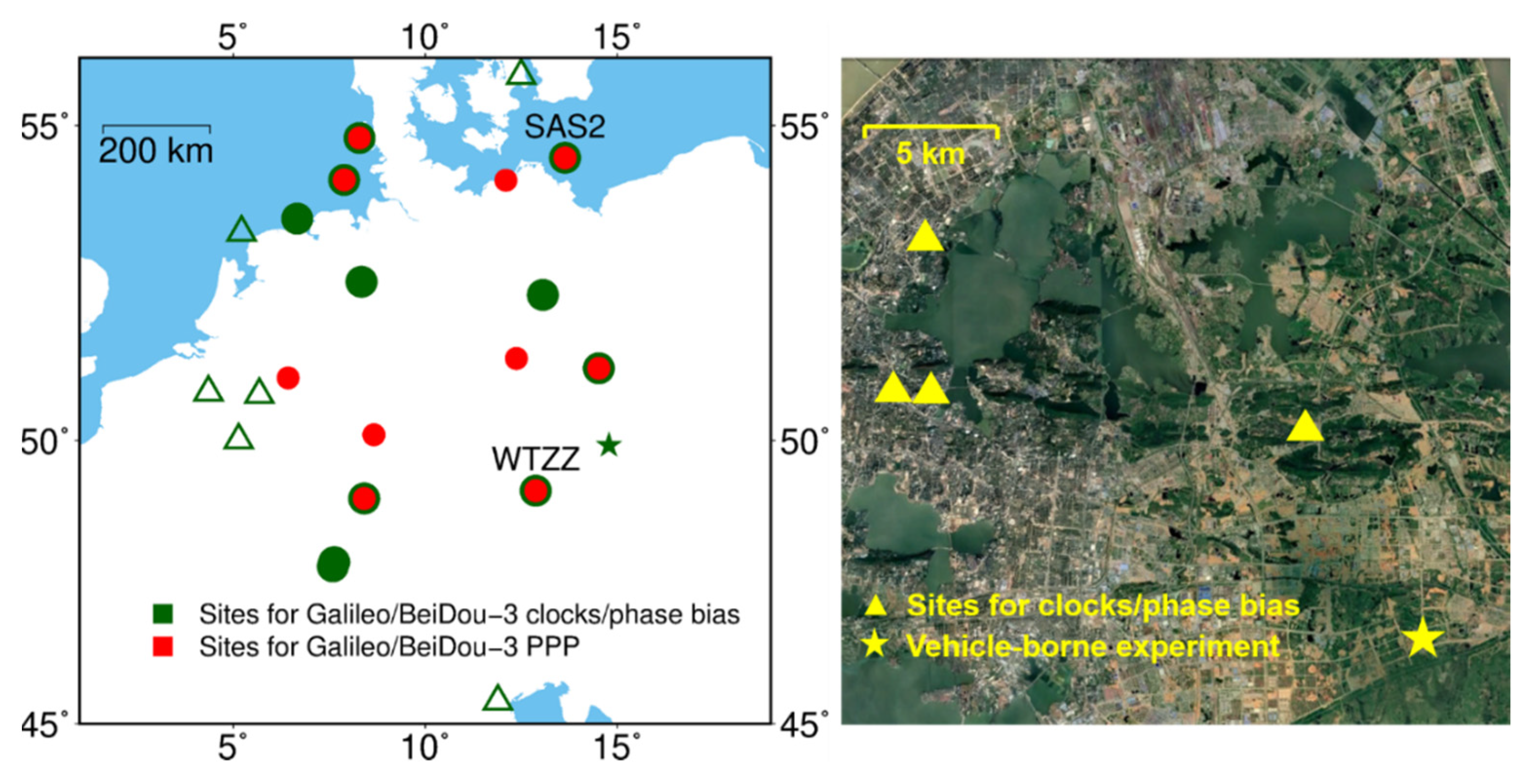
In the experiment, we first implemented triple-frequency Galileo/BeiDou-3 PPP-AR, using 31 days of 30-s data spanning days 181–211 of 2020, from 22 IGS (International GNSS Service) and EUREF Permanent Network (EPN) stations. The left panel of Figure 1 shows the station distribution. Table 2 gives the information of stations. 18 stations were used for satellite clock and phase bias estimation and 10 stations for PPP. Note that 6 stations were used for both satellite product calculation and PPP, since only 15 Javad receivers could provide all Galileo and BeiDou-3 observations. Precise orbits calculated by Wuhan University (refer to [29]) were applied and satellite clocks were self-estimated in this study. IGS Repro3 ANTEX file igsR3_2077.atx was used for correcting receiver-pair multi-frequency phase center offsets (PCO) and phase center variations (PCV) [30]. Note that igs14_2091.atx was used for satellite PCO/PCV corrections because of the lack of BeiDou-3 satellite PCOs in igsR3_2077.atx. More data processing strategies and models are displayed in Table 3.
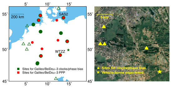
Figure 1.
The left panel shows the distribution of stations used for product calculation and PPP where cycles, triangles, and stars denote stations equipped with Javad, Septentrio, and Trimble receivers, respectively. The right panel shows the distribution of the regional network established for vehicle-borne experiment.
Table 2.
Receiver details of stations used in this study.
Table 3.
Models and parameter estimation strategies in the data processing.
A vehicle-borne experiment was implemented on day 236 of 2020 to validate rapid Galileo/BeiDou-3 triple-frequency PPP-AR in kinematic scenarios. As shown in the right panel, four temporary stations equipping Trimble Alloy receivers in Wuhan were used for satellite clock and phase bias calculation. The experiment was carried out at an open-sky environment in Wuhan and about 2 h of 30-s GNSS data was collected. A Trimble Alloy receiver was placed in the vehicle to receive multi-frequency observations, while a TRM115000 antenna was put on the roof. Note that a reference station equipped with a Trimble NETR9 was established near the experiment area. We took the short-baseline solutions to benchmark vehicle-borne PPP-AR solutions.
4. Results
In this section, PPP-WAR is first implemented where the performance of resolving multi-frequency ambiguities can be reflected directly. Sequentially, the convergence performance of PPP-AR is analyzed with respect to different satellite numbers. Finally, a vehicle-borne PPP-AR experiment is carried out to validate this fast convergence strategy.
4.1. PPP-WAR
PPP-WAR is the basis of rapid narrow-lane ambiguity resolution. In this study, we used two groups of signals to carry out PPP-WAR and PPP-AR, which are Group A: E1/E5a/E6 and B1C/B2a/B3I, and Group B: E1/E5a/E5b and B1C/B2a/B2b. Group A includes two signal combinations which have the lowest noise amplification factors (67 for Galileo and 71 for BeiDou-3), whereas Group B has larger noise amplification factors of up to 172. Note that we mark a successful convergence at the epoch where horizontal and vertical positions fall into ±5 and ±10 cm, respectively, for 10 min.
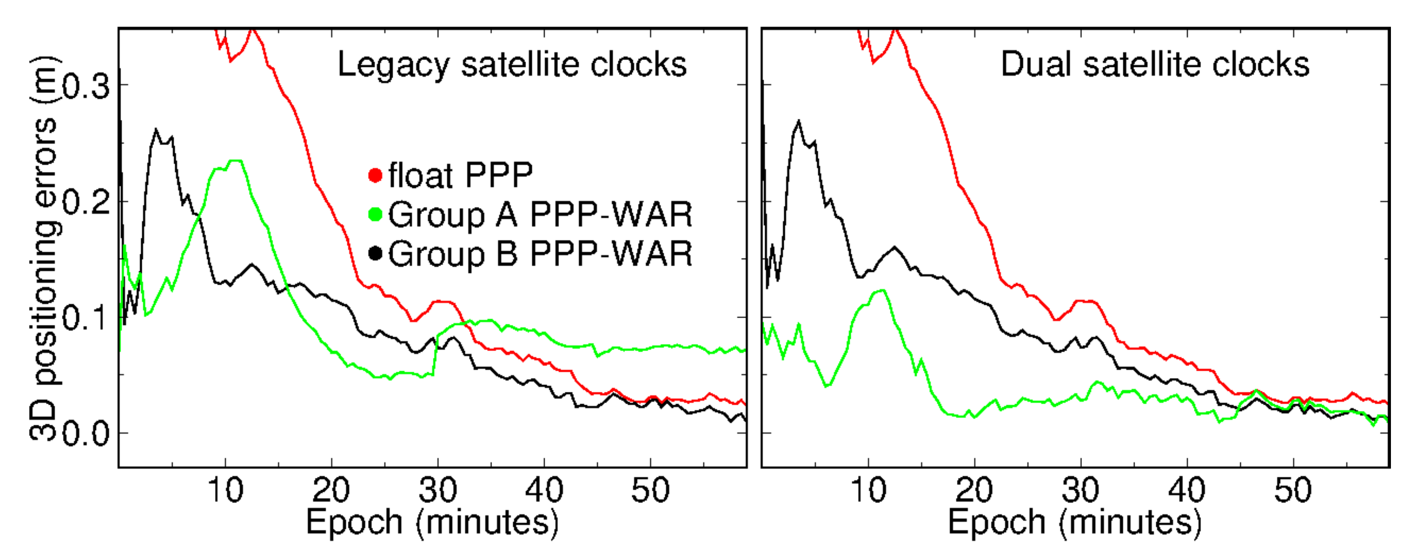
Figure 2 shows the Galileo/BeiDou-3PPP-WAR results of station WTZZ on day 183. As shown in the left panel, we first used legacy dual-frequency satellite clock products on the third-frequency observables. In this case, PPP-WAR of Group B only took 25.5 min to converge, while 36 min was required for float PPP. For Group A, unexpectedly, PPP-WAR could not converge successfully even within one hour. In our theoretical derivation, the lower noise of Group A combinations should lead to faster convergence than Group B. Ref. [34] demonstrated that multi-frequency PPP-AR solutions were more vulnerable than float solutions to some frequency-specific errors (e.g., antenna phase centers, IFCB); they demonstrated that even a bias of several millimeters could deteriorate multi-frequency PPP-AR convergence performance. In this case, we further implemented PPP-WAR using dual satellite clocks (refer to (5)), which is shown in the right panel. We have observed a milimeter-level frequency-dependent bias between E1/E5a and E6. Similar biases are existing between B1C/B2a and B3I. This is not mentioned in the former publications, but can deteriorate multi-frequency PPP-AR. We infer that these biases may be caused by IFCB, satellite, and receiver PCO errors (for more details, please refer to the Discussion section). Since the network we used was quite small, we expected that those bias could be absorbed into the second satellite clocks.

Figure 2.
PPP-WAR solutions at station WTZZ at UTC 9:00 on day 183 of 2020.
The right panel shows the PPP-WAR time series based on dual satellite clocks, where we can see the systematic error of the green line has been eliminated. After applying dual satellite clocks, Group A-based PPP-WAR converged successfully within 3.5 min, while the other two solutions showed insignificant improvements. Table 4 further gives the statistic of 1-month solutions. We can see that the convergence time and positioning accuracy of ambiguity-float PPP were almost unchanged no matter what frequency combinations or satellite clocks were used. However, for Group A and Group B using legacy satellite clocks, the mean convergence time could be shortened from about 32 min to 26.3 and 25.1 min, respectively, after resolving two wide-lane ambiguities. If dual satellite clocks were used, the fastest PPP-WAR convergence of 18.2 min was achieved based on Group A. Compared with Group A, the performance of Group B PPP-WAR based on these two clock models was similar, which is because both E5a/E5b and B2a/B2b are BOC (binary offset carrier) signals. Owing to the similar characteristics of BOC signals, the frequency-dependent biases can be well eliminated in extra-wide-lane observables. Moreover, only Group A PPP-WAR under the dual clocks model could converge in 1 h at 90th percentile. Table 4 also shows the mean positioning root mean square (RMS) error of the first 10 min of all solutions. For cases using legacy satellite clocks, though Group A PPP-WAR converged slower than Group B counterpart, Group A achieved a higher positioning precision of 6, 8, and 14 cm in the first ten minutes. This also indicated that systematic errors might be caused by Group A PPP-WAR using legacy satellite clocks.
Table 4.
PPP-WAR convergence times and positioning precisions for one month of solutions. Mean, 50th, and 90th percentiles of the convergence time are given and delimited by two slashes. “-“ denotes those solutions that did not converge within 1 h. Note that only the first ten minutes of each solution was used to calculate the positioning RMS.
4.2. PPP-AR
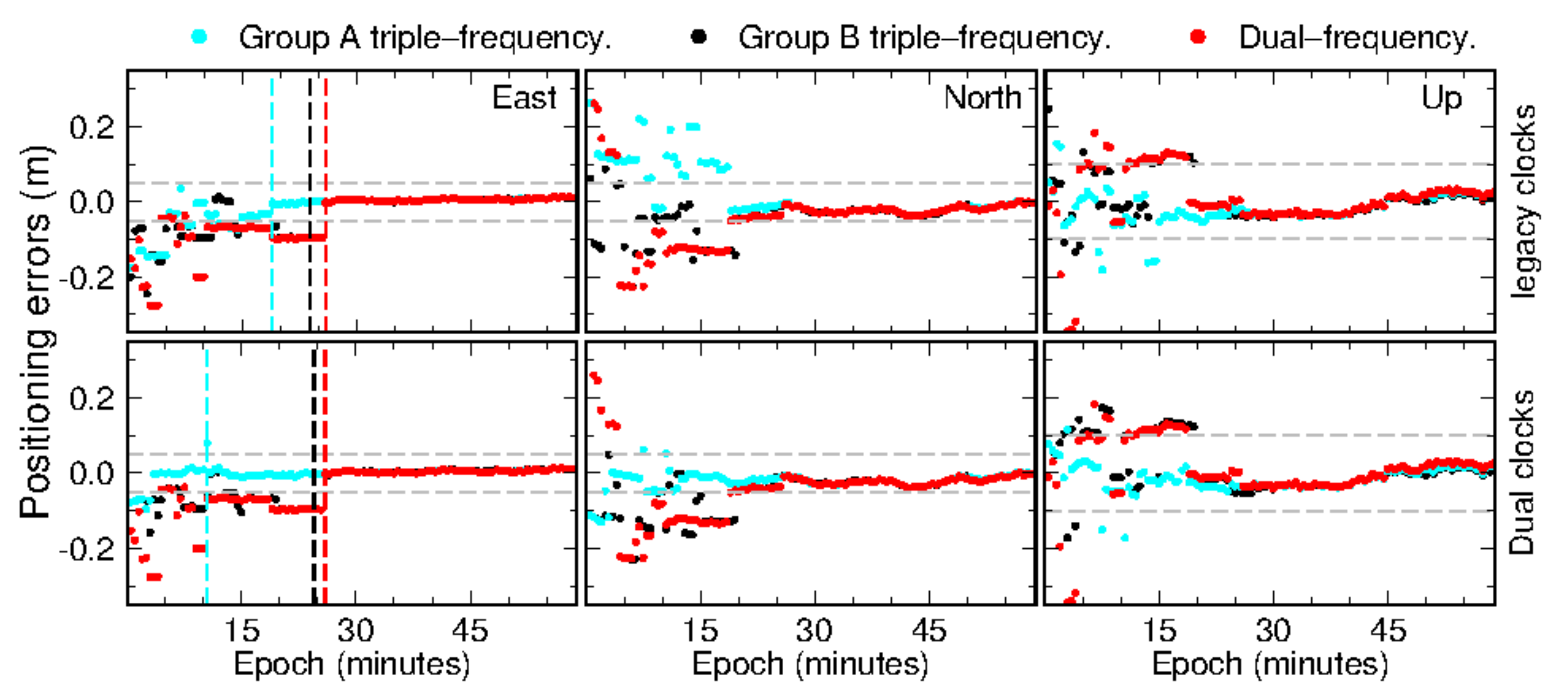
In this section, we discuss triple-frequency PPP-AR performance based on Groups A and B combination observations. Similar to the strategies for PPP-WAR, both legacy and dual satellite clocks were tried. Figure 3 shows the 1-h PPP-AR solution of station SAS2 at around UTC 20:00 on day 183 of 2020. During this period, about 12 Galileo/BeiDou-3 satellites were observed and distributed in good geometry. The position dilution of precision (PDOP) value is only 1.5. The top three panels show the results calculated using legacy satellite clocks. As shown by the vertical dashed lines, dual-frequency PPP-AR needs 26 min to converge. By resolving triple-frequency ambiguities, the convergence times of PPP-AR are significantly shortened, to 19 and 24 min for solutions based on Groups A and B, respectively. Interestingly, the introduction of dual satellite clocks makes PPP-AR under Group A converge successfully within 10.5 min, showing an improvement of 45% compared with that based on legacy clocks.

Figure 3.
One-hour PPP-AR solutions of SAS2 on UTC 20:00, day 183 of 2020. The dashed gray lines are ±5 cm for horizontal directions and ±10 cm for vertical direction, while the vertical dashed lines mark the convergence epoch of each solution.
The mean, 50th, and 90th percentiles of convergence time for all stations over the month are shown in Table 5. Dual-frequency PPP-AR needs 11.6 min on average to converge successfully while all triple-frequency solutions can achieve convergence within 9 min. Meanwhile, compared with the convergence of triple-frequency PPP-AR under Group B, an improvement of 10% is induced after applying combination Group A. This improvement was further enlarged to 36% when we introduced dual satellite clocks. Specifically, Group A PPP-AR could converge within 5.6 min, achieving a positioning accuracy of 2 cm, 4 cm, and 8 cm for the east, north, and up components, respectively, in the first 10 min. Similarly, ref. [16] resolved PPP ambiguity successfully in 6 min on average, but they used more constellations: GPS/Galileo/BeiDou-2/QZSS. Ref. [21] carried out Galileo-only PPP-AR and achieved a mean convergence time of 15.5 min by resolving E1/E5a/E6 ambiguities. We can see that the combination of Galileo and BeiDou-3 is necessary to accomplish convergence in several minutes, even if optimal signals combination is applied.
Table 5.
Convergence times of PPP-AR over all solutions. Mean, 50th, and 90th percentiles are given, delimited by two slashes. The fourth column is the improvement of solutions using dual clocks compared with dual-frequency counterparts.
It is worth noting that both Galileo and BeiDou-3 were not fully operational in our experiment period and about 30% solutions were processed in the case of less than 10 satellites. We thus picked the solutions where more than 10 satellites were involved into PPP. From the last two rows of Table 5, we can see that the difference between Group A and Group B PPP-AR is still insignificant. Fortunately, dual satellite clocks can still contribute in this case. For the Group A solution, an improvement of 39% was achieved by introducing the second clocks. On the contrary, the results of Group B PPP-AR were the same no matter what clock products were used. In this case, the 90th and 50th percentile convergence times of all strategies are shorter than 15 min and 5 min, respectively. Specifically, 50% of Group A PPP-AR using dual clocks can converge in 30 s.
Figure 4 shows the distribution of the convergence time of PPP-AR based on dual satellite clocks. Note that we assume the convergence time is 60 min if a solution fails to converge within 1 h. The percentage of un-converged solutions is marked in the right-top corner of each panel and 99% of Group A PPP-AR could achieve initialization within 1 h. From panels (a–c), we can see that 70%, 58%, and 43% of solutions of Group A/Group B triple-frequency and dual-frequency PPP-AR accomplished convergence in 5 min. As for panels (d–f), we picked the solutions where more than 10 satellites were used. In this case, 81% of Group A triple-frequency PPP-AR solutions converged successfully in 5 min. Meanwhile, it is promising that 62% of solutions achieved convergence within 1 min. Though the experiments were carried out with a regional network due to the limited number of eligible stations, we did not use any atmosphere corrections to augment PPP. Therefore, it is possible for global multi-frequency PPP-AR users to converge in 10 min at any time.
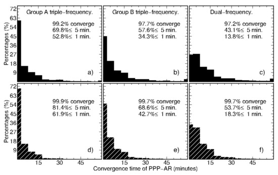
Figure 4.
Distribution of PPP-AR convergence times with respect to dual satellite clock cases. Panels (a–c) display the results of Group A triple-frequency, Group B triple-frequency, and dual-frequency PPP-AR, respectively, while (d–f) are the corresponding distributions calculated with the solutions that observed more than 10 satellites. The percentages of the solutions converging successfully in 1 h, 5 min, and 1 min are also given in the right-top corner of each panel.
4.3. Vehicle-Borne Experiment
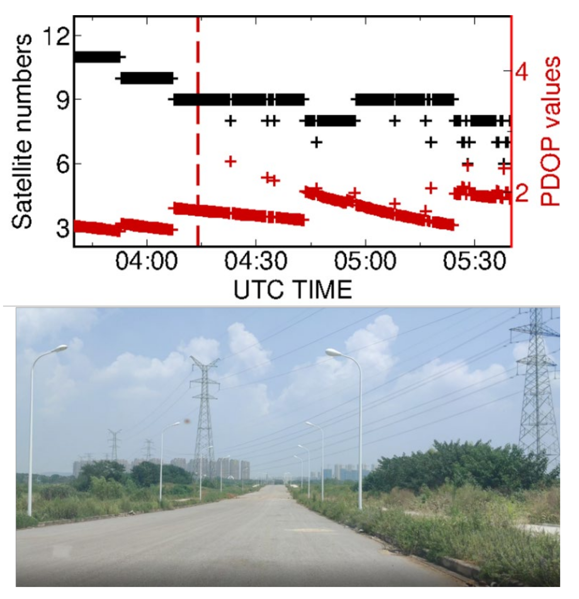
A vehicle-borne experiment on day 236, 2020, was carried out in Wuhan city, China. Overall, 2 h of 30-s multi-frequency Galileo/BeiDou-3 observations were collected using Trimble Alloy receivers. In the first 30 min, the vehicle was static; we drove back and forth at a speed of about 30 km/h on an open-sky-view road for about 1.5 h (see Figure 5). As shown in the bottom panel, the experiment environment had a wide view, while there were some high voltage overhead power lines crossing over the road. The top panel gives the satellite numbers and PDOP values of Galileo and BeiDou-3 during this period. We can see that there were nine satellites on average during the experiment period and the satellite number and PDOP values kept stable when the vehicle was staying static. However, frequent loss of satellites occurred once the vehicle started to move. Specifically, there were only six satellites left at some epochs.

Figure 5.
The top panel shows the satellite numbers and PDOP values during experiment period. The dotted red line marks the epoch when the vehicle started moving. The bottom panel is the snapshot of the experiment environment nearing to the high voltage overhead power lines.
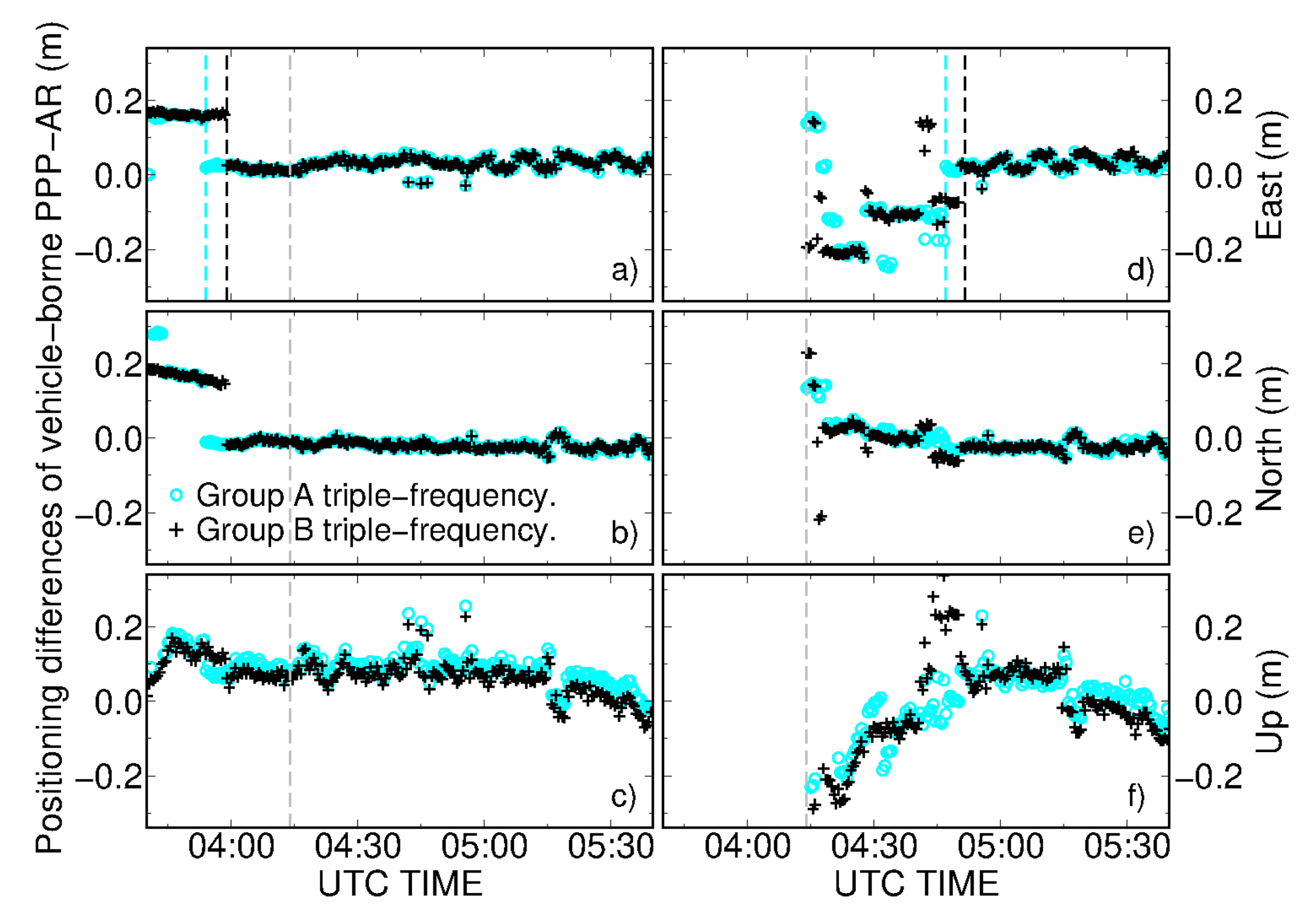
Figure 6 displays the positioning differences of triple-frequency PPP-AR based on kinematic observations. All solutions in this section were calculated with dual clocks. The benchmark solutions were calculated with the short-baseline RTK, and over 95% of epochs were fixed successfully. Panels (a–c) were processing from the beginning of the 2-h period. In this case, the vehicle kept static during the first 30 min to make the PPP-AR converge. As shown by the black curves, it took 19 min for Group B PPP-AR to resolve ambiguities, even if there were about 10 satellites in view. The convergence time was improved to 14 min after we applied Group A signal combinations, showing an improvement rate of 26%. We recognize that this convergence time is much longer than those in Table 5, even if the observation condition is comparable to the static stations. One of the possible reasons is that 40% of the observed satellites in the kinematic period were in low elevation (lower than 30°). Another reason is that the precise products, such as dual satellite clocks and phase biases, were calculated by a local network containing only 4 stations (Figure 1). These stations were not enough to guarantee a high precision of phase bias product. Furthermore, we observed that the positioning differences of ambiguity-fixed PPP were degraded as the satellite number suddenly decreased.
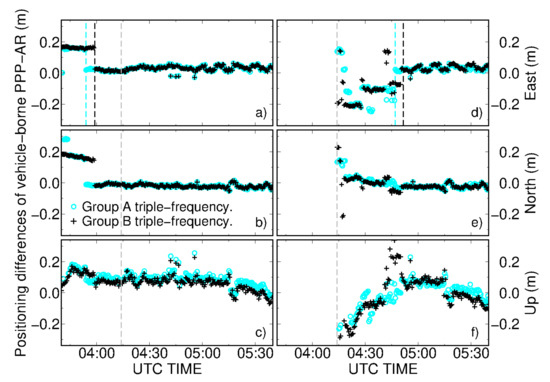
Figure 6.
Positioning differences of east, north, and up components between vehicle-borne PPP-AR and short-baseline solutions. Panels (a–c) are solutions which were processed from the beginning of the static period while in panels (d–f) we only processed the epochs when the vehicle was moving. Dashed cyan and black lines represent the epochs when Group A and Group B triple-frequency PPP-AR converged successfully. Finally, dashed gray lines mark the epoch from which the vehicle began to move.
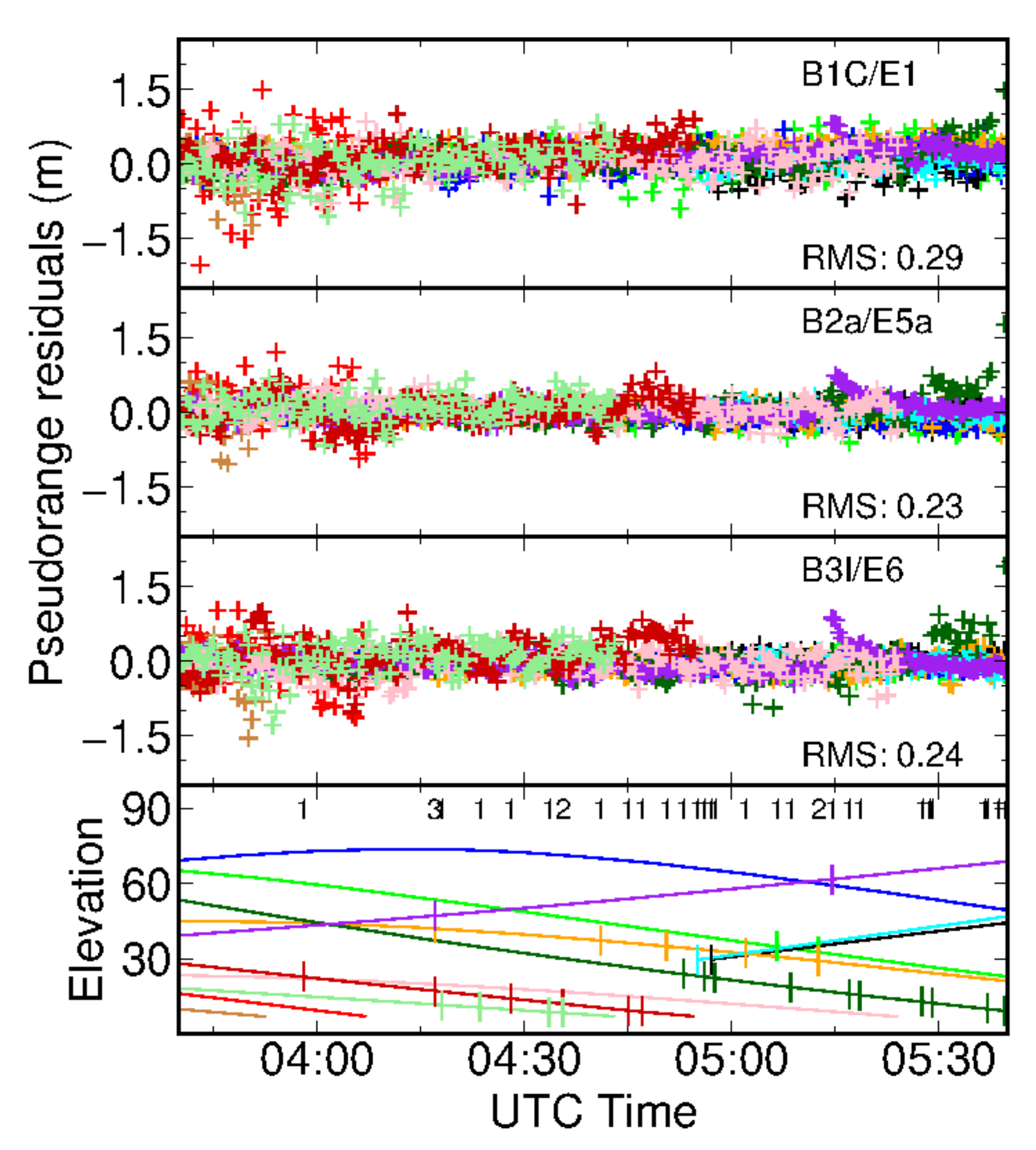
Moreover, it is interesting to investigate the differences of PPP convergence performance between static and kinematic receivers. Therefore, we tried PPP-AR after the vehicle begun to moving; results are shown in panels (d–f) of Figure 6. In movement, vehicle-borne PPP-AR achieved convergence in 33 and 37.5 min for Group A and Group B, respectively. This convergence is even slower than those based on a static vehicle. We analyzed the observation residuals; cycle slips occurred during the whole period, which are shown in Figure 7. Taking Group A PPP-AR as an example, the RMS of pseudorange residuals are 0.29 m, 0.23 m, and 0.24 m for E1/B1C, E5a/B2a, and E6/B3I signals, respectively. 99% of pseudorange residuals fall into ±2 m and no obvious bias can be found. However, frequent loss of satellites occurred during the movement of vehicle. Too many cycle slips may have compromised narrow-lane ambiguity resolution, even though most of them occurred with low-elevation satellites.
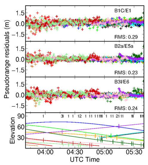
Figure 7.
Galileo/BeiDou-3 satellites pseudorange residuals of Group A PPP-AR and the elevation angles. Cycle slips are marked with short vertical lines on each elevation curve. The number of satellites with cycle slips at each epoch is marked in the bottom panel.
5. Discussion
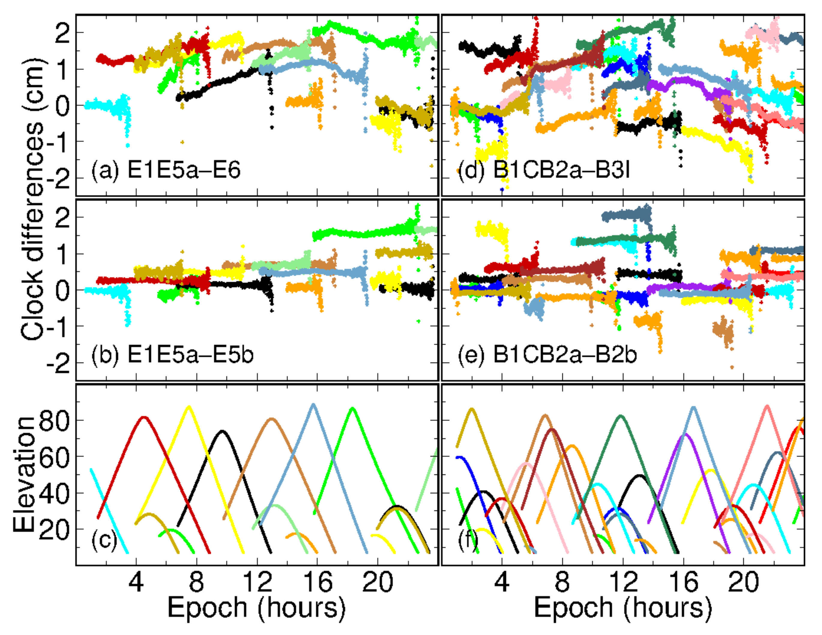
In this study we processed triple-frequency data based on legacy and dual satellite clocks, respectively. When legacy dual-frequency satellite clocks were applied, some systematic offsets were observed among both PPP-WAR and PPP-AR positioning results, especially for those based on B1C/B2a/B3I and E1/E5a/E6 signal combinations. We inferred that there were some frequency-dependent biases (e.g., IFCB, multi-frequency PCO errors) left in the data processing model. It has been demonstrated that these frequency-dependent biases could be magnified after forming combined observables (i.e., PPP-WAR) [34]. In this case, even a bias of several millimeters can threaten PPP-AR. We thus estimated a second satellite clock on the third-frequency observables to absorb potential IFCBs and remained PCO errors. A significant improvement was achieved on both PPP-WAR and PPP-AR based on Group A signals after introducing dual satellite clocks. Figure 8 shows the differences of satellite clocks estimated on legacy dual-frequency observations and the third frequency signals. From panel (a) and (d), we can see that some time-varying biases were lumped into the second satellite clocks. The peak-to-peak amplitudes of these biases can reach up to 1 cm. We recognize that some of the biases for BeiDou-3 satellites might be IFCBs, which are negligible for ambiguity-float PPP owing to its millimeter-level magnitude. Meanwhile, ref. [35] also stated that BeiDou-3 satellites had small IFCBs with peak-to-peak amplitude of 1 cm.
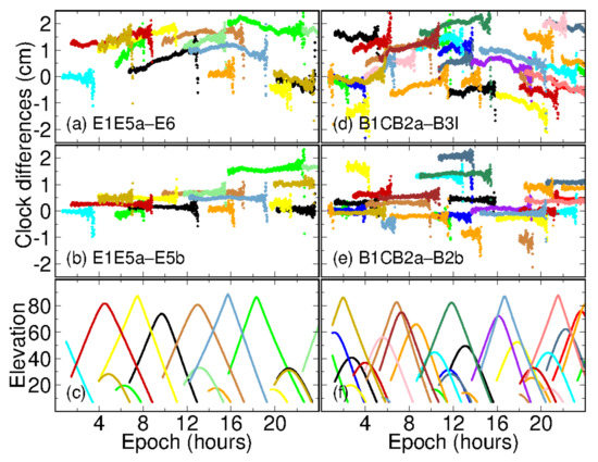
Figure 8.
Clock differences between legacy satellite L1/L2 clock and the clock on the third-frequency L3. Panels (a,b) denote the results of Galileo E1/E5a/E6 and E1/E5a/E5b, while panel (c) gives the elevation angles of Galileo satellites at stations WTZZ. Panels (d–f) are the results for BeiDou-3 counterpart.
On the other hand, PCO errors left on the third frequency observations can be another frequency-dependent bias, even if we have applied multi-frequency receiver antenna file igsR3_2077.atx. We can see that there are some elevation-dependent variations in panel (a) and (b). We have found that the disagreement of multi-frequency receiver-pair PCOs can reach to 1–3 mm between those provided by EPN (refer to ftp://epncb.oma.be/pub/station/general, accessed on 13 October 2021) and igsR3_2077.atx. Moreover, it has been noted that the satellite-pair Galileo z-PCOs provided by GFZ (GFZ (GeoForschungsZentrum) and DLR (Deutsches Zentrum für Luft und Raumfahrt) differed by 20 cm [36]. By estimating the second satellite clocks among a comparable small area in this study, these PCO residuals were partly absorbed by the second satellite clocks. It is interesting that there are no significant time-varying biases among the differences between Group B combination clocks (refer to panel (b) and (e)). This can be understood in terms of the similar characteristics of BOC signals. Therefore, to uncover the contribution of multi-frequency signals to PPP, frequency-dependent biases such as IFCBs and PCOs errors should be well considered, even if they are negligible in dual-frequency data processing.
6. Conclusions
In this study, we investigate the performance of multi-frequency PPP-AR using BeiDou-3/Galileo B1C/B2a/B3I and E1/E5a/E6 signal combinations. With the emergence of Galileo E6 and BeiDou-3 new-generation B1C/B2a/B2b signals, we identified above two signal combinations (termed “Group A”) that have very small noise amplification factors (67 and 71) to benefit rapid PPP-AR. We thus aim to overcome the long-convergence issue of PPP with multi-frequency signals and improved precise products such as satellite clocks. We processed 1 month of data from 22 stations and obtained promising results. If more than 10 satellites are involved, 62% of triple-frequency PPP-AR converge successfully within 1 min by introducing Group A signal combinations. We also found some potential issues present in multi-frequency PPP data processing, which prove to be harmful to PPP-AR convergence.
The rapid resolution of narrow-lane ambiguities depends on the positioning errors of PPP-WAR. In this case, we first evaluate the performance of PPP-WAR based on Group A, and the other signal combinations B1C/B2a/B2b and E1/E5a/E5b, which have a larger noise amplification factor of 172 (termed as “Group B”). On average, it took about 32 min for ambiguity-float PPP to converge. Once the extra-wide/wide-lane ambiguities were resolved, a positioning accuracy of 10–20 cm can be achieved by PPP-WAR in several epochs. As a result, the convergence time is shortened to 25 min for PPP-WAR using Group B signal combinations Galileo E1/E5a/E5b and BeiDou-3 B1C/B2a/B2b. If E1/E5a/E6 and B1C/B2a/B3I combinations were used, only 18 min were required for PPP-WAR convergence. The triple-frequency PPPs were implemented using dual satellite clock products [24]. Some potential bias such as IFCB and PCO aligning errors of multi-frequency signals have significant effects on triple-frequency PPP. For Group A, PPP-WAR using legacy satellite clocks, the average convergence time reaches 26.3 min, which is 1.4 times those using dual clock products. We speculate that IFCB and part of the receiver-pair PCO errors can be absorbed by estimating a second satellite clock on the third frequency.
The lower-noise signal combinations of Group A make PPP-AR possible to converge in 1 or 2 min. In this study, we achieved PPP-AR convergence in 5.6 min on average using Galileo and BeiDou-3 Group A combinations, showing an improvement of 36% and 55% compared with Group B and dual-frequency PPP-AR counterparts. About 53% of Group A PPP-AR accomplished convergence within 1 min, compared to only 34% for those using Group B combinations. Considering that Galileo and BeiDou-3 satellites are not fully operational yet, good geometry conditions could not be ensured within all the solutions. We thus analyzed solutions where more than 10 satellites were observed to give an initial assessment for PPP-AR using the full Galileo and BeiDou-3 constellation. If there were more than 10 satellites involved, Group A PPP-AR could converge in 3 min. Of these PPP-AR solutions, 62% achieved their convergence within 1 min. On the contrary, ref. [16] achieved the convergence of 63% of GPS/Galileo/BeiDou-2/QZSS solutions within up to 5 min, based on combinations which amplified the noise by over 100 times.
A vehicle-borne experiment was designed to validate this approach in kinematic scenarios. We investigated PPP-AR convergence performance based on static and kinematic scenarios. When the vehicle remained static, it took 14 min for the successful convergence of Group A PPP-AR and 19 min for the high-noise counterpart. As for PPP-AR during the motion of vehicle, a longer time of 33 min was required even for solutions based on Group A. The slower convergence during the movement of vehicle was caused by the frequent loss of the satellites. However, an improvement of 12% was still observed by comparing the convergence of the Group A and B PPP-AR solutions.
Author Contributions
Conceptualization: J.G.; Software: J.G. and G.L.; Data analysis: Q.Z. and K.Z; Writing: J.G. and G.L.; Editing: J.G., Q.Z., G.L. and K.Z. All authors have read and agreed to the published version of the manuscript.
Funding
This study is funded by the National Key Research and Development Program of China (2018YFC1503601) and the National Science Foundation of China (42025401).
Institutional Review Board Statement
Not applicable.
Informed Consent Statement
Not applicable.
Data Availability Statement
All raw GNSS data were collected from IGS (ftp://gdc.cddis.eosdis.nasa.gov, accessed on 13 October 2021) and EPN (ftp://igs.bkg.bund.de/EUREF/, accessed on 13 October 2021).
Acknowledgments
We thank the IGS (International GNSS Service) and EPN (EUREF Permanent Network) for the multi-GNSS data and the high-quality satellite products. All data were processed by PRIDE PPP-AR. The computation work was accomplished on the high-performance computing facility of Wuhan University.
Conflicts of Interest
The authors declare no conflict of interest.
References
- Malys, S.; Jensen, P.A. Geodetic point positioning with GPS carrier beat phase data from the CASA UNO Experiment. Geophys. Res. Lett. 1990, 17, 651–654. [Google Scholar] [CrossRef]
- Zumberge, J.F.; Heflin, M.B.; Jefferson, D.C.; Watkins, M.M.; Webb, F.H. Precise point positioning for the efficient and robust analysis of GPS data from large networks. J. Geophys. Res. Space Phys. 1997, 102, 5005–5017. [Google Scholar] [CrossRef] [Green Version]
- An, X.; Meng, X.; Jiang, W. Multi-constellation GNSS precise point positioning with multi-frequency raw observations and dual-frequency observations of ionospheric-free linear combination. Satell. Navig. 2020, 1, 1–13. [Google Scholar] [CrossRef]
- Bisnath, S.; Gao, Y. Current state of precise point positioning and future prospects and limitations. In Observing Our Changing Earth; Sideris, M.G., Ed.; Springer: Berlin/Heidelberg, Germany, 2009; pp. 615–623. [Google Scholar]
- Teunissen, P.J.G.; Odolinski, R.; Odijk, D. Instantaneous BeiDou+GPS RTK positioning with high cut-off elevation angles. J. Geod. 2014, 88, 335–350. [Google Scholar] [CrossRef]
- Wübbena, G.; Schmitz, M.; Bagge, A. PPP-RTK: Precise point positioning using state-space representation in RTK networks. In Proceedings of the ION GNSS 2005, Institute of Navigation, Inc., Fairfax, VA, USA, 13–16 September 2005; pp. 2584–2594. [Google Scholar]
- Geng, J.; Meng, X.; Dodson, A.H.; Ge, M.; Teferle, F.N. Rapid re-convergences to ambiguity-fixed solutions in precise point positioning. J. Geod. 2010, 84, 705–714. [Google Scholar] [CrossRef] [Green Version]
- Zhang, B.; Chen, Y.; Yuan, Y. PPP-RTK based on undifferenced and uncombined observations: Theoretical and practical aspects. J. Geod. 2019, 93, 1011–1024. [Google Scholar] [CrossRef]
- Hein, G.W. Status, perspectives and trends of satellite navigation. Satell. Navig. 2020, 1, 22. [Google Scholar] [CrossRef]
- Geng, J.; Shi, C. Rapid initialization of real-time PPP by resolving undifferenced GPS and GLONASS ambiguities simultaneously. J. Geod. 2017, 91, 1–14. [Google Scholar] [CrossRef]
- Liu, Y.; Lou, Y.; Ye, S.; Zhang, R.; Song, W.; Li, Q. Assessment of PPP integer ambiguity resolution using GPS, GLONASS and BeiDou (IGSO, MEO) constellations. GPS Solut. 2017, 21, 1647–1659. [Google Scholar] [CrossRef]
- Hatch, R.; Jung, J.; Enge, P.; Pervan, B. Civilian GPS: The Benefits of Three Frequencies. GPS Solut. 2000, 3, 1–9. [Google Scholar] [CrossRef]
- Geng, J.; Bock, Y. Triple-frequency GPS precise point positioning with rapid ambiguity resolution. J. Geod. 2013, 87, 449–460. [Google Scholar] [CrossRef]
- Melbourne, W.G. The case for ranging in GPS-based geodetic systems. In Proceedings of the 1st International Symposium on Precise Positioning with the Global Positioning System, Rockville, MD, USA, 15–19 April 1985; pp. 373–386. [Google Scholar]
- Wübbena, G. Software developments for geodetic positioning with GPS using TI-4100 code and carrier measurements. In Proceedings of the 1st International Symposium on Precise Positioning with the Global Positioning System, Rockville, MD, USA, 15–19 April 1985; pp. 403–412. [Google Scholar]
- Geng, J.; Guo, J.; Meng, X.; Gao, K. Speeding up PPP ambiguity resolution using triple-frequency GPS/BeiDou/Galileo/QZSS data. J. Geod. 2020, 94, 1–15. [Google Scholar] [CrossRef] [Green Version]
- Xiao, G.; Li, P.; Gao, Y.; Heck, B. A Unified Model for Multi-Frequency PPP Ambiguity Resolution and Test Results with Galileo and BeiDou Triple-Frequency Observations. Remote Sens. 2019, 11, 116. [Google Scholar] [CrossRef] [Green Version]
- Liu, G.; Zhang, X.; Li, P. Improving the performance of Galileo uncombined precise point positioning ambiguity resolution using triple-frequency observations. Remote Sens. 2019, 11, 341. [Google Scholar] [CrossRef] [Green Version]
- Duong, V.; Harima, K.; Choy, S.; Laurichesse, D.; Rizos, C. Assessing the performance of multi-frequency GPS, Galileo and BeiDou PPP ambiguity resolution. J. Spat. Sci. 2019, 65, 61–78. [Google Scholar] [CrossRef]
- Guo, J.; Xin, S. Toward single-epoch 10-centimeter precise point positioning using Galileo E1/E5a and E6 signals. In Proceedings of the ION GNSS 2019, Institute of Navigation, Miami, FL, USA, 16–20 September 2019; pp. 2870–2887. [Google Scholar]
- Psychas, D.; Teunissen, P.; Verhagen, S. A Multi-Frequency Galileo PPP-RTK Convergence Analysis with an Emphasis on the Role of Frequency Spacing. Remote Sens. 2021, 13, 3077. [Google Scholar] [CrossRef]
- Geng, J.; Guo, J. Beyond three frequencies: An extendable model for single-epoch decimeter-level point positioning by exploiting Galileo and BeiDou-3 signals. J. Geod. 2020, 94, 14. [Google Scholar] [CrossRef]
- Odijk, D.; Zhang, B.; Khodabandeh, A.; Odolinski, R.; Teunissen, P. On the estimability of parameters in undifferenced, uncombined GNSS network and PPP-RTK user models by means of S-system theory. J. Geod. 2016, 90, 15–44. [Google Scholar] [CrossRef]
- Guo, J.; Geng, J. GPS satellite clock determination in case of inter-frequency clock biases for triple-frequency precise point positioning. J. Geod. 2017, 92, 1133–1142. [Google Scholar] [CrossRef]
- Ge, M.; Gendt, G.; Rothacher, M.; Shi, C.; Liu, J. Resolution of GPS carrier-phase ambiguities in Precise Point Positioning (PPP) with daily observations. J. Geod. 2008, 82, 389–399. [Google Scholar] [CrossRef]
- Laurichesse, D.; Mercier, F.; Berthias, J.-P.; Broca, P.; Cerri, L. Integer ambiguity resolution on undifferenced GPS phase measurements and its application to PPP and satellite precise orbit determination. Navig. J. Inst. Navig. 2009, 56, 135–149. [Google Scholar] [CrossRef]
- Geng, J.; Meng, X.; Dodson, A.H.; Teferle, F.N. Integer ambiguity resolution in precise point positioning: Method comparison. J. Geod. 2010, 84, 569–581. [Google Scholar] [CrossRef] [Green Version]
- Teunissen, P.J.G. The least-squares ambiguity decorrelation adjustment: A method for fast GPS integer ambiguity estimation. J. Geod. 1995, 70, 65–82. [Google Scholar] [CrossRef]
- Guo, J.; Xu, X.; Zhao, Q.; Liu, J. Precise orbit determination for quad-constellation satellites at Wuhan University: Strategy, result validation, and comparison. J. Geod. 2016, 90, 143–159. [Google Scholar] [CrossRef]
- IGS AC Coordinator. Conventions and Modeling for Repro3. 2019. Available online: http://acc.igs.org/repro3/repro3.html (accessed on 6 June 2020).
- Saastamoinen, J. Contribution to the theory of atmospheric refraction: Refraction corrections in satellite geodesy. Bull. Geod. 1973, 107, 13–34. [Google Scholar] [CrossRef]
- Boehm, J.; Niell, A.; Tregoning, P.; Schuh, H. Global Mapping Function (GMF): A new empirical mapping function based on numerical weather model data. Geophys. Res. Lett. 2006, 33, L07304. [Google Scholar] [CrossRef] [Green Version]
- Teunissen, P.J.G. The geometry-free GPS ambiguity search space with a weighted ionosphere. J. Geod. 1997, 71, 370–383. [Google Scholar] [CrossRef] [Green Version]
- Geng, J.; Guo, J.; Wang, C.; Zhang, Q. Satellite antenna phase center errors: Magnified threat to multi-frequency PPP ambiguity resolution. J. Geod. 2021, 95, 72. [Google Scholar] [CrossRef]
- Xie, X.; Fang, R.; Geng, T.; Wang, G.; Zhao, Q.; Liu, J. Characterization of GNSS signals tracked by the iGMAS network considering recent BDS-3 satellites. Remote Sens. 2018, 10, 1736. [Google Scholar] [CrossRef] [Green Version]
- Steigenberger, P.; Fritsche, M.; Dach, R.; Schmid, R.; Montenbruck, O.; Uhlemann, M.; Prange, L. Estimation of satellite antenna phase center offsets for Galileo. J. Geod. 2016, 90, 773–785. [Google Scholar] [CrossRef]

Publisher’s Note: MDPI stays neutral with regard to jurisdictional claims in published maps and institutional affiliations. |
© 2021 by the authors. Licensee MDPI, Basel, Switzerland. This article is an open access article distributed under the terms and conditions of the Creative Commons Attribution (CC BY) license (https://creativecommons.org/licenses/by/4.0/).