Article

Classifying Crop Types Using Two Generations of Hyperspectral Sensors (Hyperion and DESIS) with Machine Learning on the Cloud

U.S. Geological Survey, Western Geographic Science Center, Flagstaff, AZ 86001, USA
*
Author to whom correspondence should be addressed.
Remote Sens. 2021, 13(22), 4704; https://doi.org/10.3390/rs13224704
Submission received: 29 September 2021 / Revised: 30 October 2021 / Accepted: 12 November 2021 / Published: 21 November 2021

Abstract

:
Advances in spaceborne hyperspectral (HS) remote sensing, cloud-computing, and machine learning can help measure, model, map and monitor agricultural crops to address global food and water security issues, such as by providing accurate estimates of crop area and yield to model agricultural productivity. Leveraging these advances, we used the Earth Observing-1 (EO-1) Hyperion historical archive and the new generation DLR Earth Sensing Imaging Spectrometer (DESIS) data to evaluate the performance of hyperspectral narrowbands in classifying major agricultural crops of the U.S. with machine learning (ML) on Google Earth Engine (GEE). EO-1 Hyperion images from the 2010–2013 growing seasons and DESIS images from the 2019 growing season were used to classify three world crops (corn, soybean, and winter wheat) along with other crops and non-crops near Ponca City, Oklahoma, USA. The supervised classification algorithms: Random Forest (RF), Support Vector Machine (SVM), and Naive Bayes (NB), and the unsupervised clustering algorithm WekaXMeans (WXM) were run using selected optimal Hyperion and DESIS HS narrowbands (HNBs). RF and SVM returned the highest overall producer’s, and user’s accuracies, with the performances of NB and WXM being substantially lower. The best accuracies were achieved with two or three images throughout the growing season, especially a combination of an earlier month (June or July) and a later month (August or September). The narrow 2.55 nm bandwidth of DESIS provided numerous spectral features along the 400–1000 nm spectral range relative to smoother Hyperion spectral signatures with 10 nm bandwidth in the 400–2500 nm spectral range. Out of 235 DESIS HNBs, 29 were deemed optimal for agricultural study. Advances in ML and cloud-computing can greatly facilitate HS data analysis, especially as more HS datasets, tools, and algorithms become available on the Cloud.

1. Introduction

Classifying agricultural crops accurately is crucial for addressing the challenges of global food and water security [1]. Remote sensing (RS) allows us to non-destructively study crops at large spatial and temporal extents. However, crop classification with RS is challenging due to high spectral variability within crop types across: crop management practices, watering methods (e.g., irrigated or rainfed), phenological differences, geographic locations, and climatic factors. Hyperspectral (HS) remote sensing captures data as hundreds of narrowbands, opening up possibilities for advancing the study and classification of agricultural crops [1,2,3,4,5]. HS narrowbands (HNBs) and HS vegetation indices (HVIs) have been used successfully over decades to classify crops, model crop photosynthetic and non-photosynthetic fractional cover, and estimate crop characteristics [1,3,6,7,8,9,10,11,12,13].
There are challenges in using HS data [1,10,11,14,15,16], including finding ways to store and process large volumes of data [17], minimize data redundancy, and acquire high-quality training and validation data with high signal to noise ratio [1,5,18]. However, there are ways to combat these challenges. For example, one way to minimize data redundancy and decrease data volume is through band selection. Recent research [2,3,4,5,11,12,17,19,20,21,22] has shown as much as 80% of HNBs can be redundant in Earth Observing1 (EO-1) Hyperion data in the study of agricultural crops. Band selection can also reduce noise (with noisy-band removal) and save time and computing resources. Advances in satellite sensor-based big-data analytics, machine learning, and cloud-computing [1,14,18,23,24,25] also facilitate HS analysis by providing a fast and reliable way to process large volumes of data [18,26,27,28,29,30,31,32,33], enabling real-time decision-making to support next generation agricultural practices [25].
The increasing availability of HS data from spaceborne platforms [1,16,34,35] makes this the ideal time to capitalize on these technological advancements. Recently launched sensors include CHRIS/PROBA, the Hyperspectral Imager (HySI) on the Indian Microsatellite-1 (IMS-1), the Hyperspectral Imager for the Coastal Ocean (HICO), the Italian PRecursore IperSpettrale della Missione Applicativa (PRISMA), and Germany’s Deutsches Zentrum für Luftund Raumfahrt (DLR) Earth Sensing Imaging Spectrometer (DESIS) [1,36]. In addition, upcoming sensors include Germany’s Environmental Mapping and Analysis Program (EnMAP), the Israeli and Italian Spaceborne Hyperspectral Applicative Land and Ocean Mission (SHALOM), and NASA’s Surface Biology and Geology (SBG) mission [1,37]. DESIS is onboard the Multiple User System for Earth Sensing Facility (MUSES) platform on the International Space Station (ISS) [38]. It acquires data from 400 to 1000 nanometers (nm) in discrete 2.55 nm bandwidths in 235 spectral bands [39].
A comparison of new generation DESIS hyperspectral data with established older generation Hyperion data leveraging advances in machine learning and cloud-computing is of considerable interest and value. The narrow bandwidth of 2.55 nm (relative to 10 nm for Hyperion) and higher signal to noise ratio (unitless) of DESIS (Table 1) may make significant differences in capturing and differentiating the subtle changes in plant quantities and characteristics. On the other hand, the wider spectral range of Hyperion (Table 1) may be more advantageous for crop classification.
The development of hyperspectral libraries has been used extensively for various classification applications including vegetation, minerals, and pigments [40,41,42,43]. The use of crop hyperspectral libraries to analyze crop characteristics is an evolving area of research [44,45,46,47]. The availability of large libraries is crucial for training and validating machine learning classification models. Several classification methods such as the supervised pixel-based random forest and support vector machines or unsupervised pixel-based statistical ISOCLASS clustering exist. In addition to sensor comparisons, obtaining clarity about the strengths and limitations of these classification methods and approaches for classifying agricultural crops is of great importance.
Thus, this study provides a number of novelties that will advance our understanding of hyperspectral data by examining: how a narrow bandwidth of 2.55 nm can help improve crop classification and characterization; how a new generation hyperspectral sensor (DESIS) compares with an old generation hyperspectral sensor (Hyperion) in the study of agricultural crops; how spectral signatures of some of the major world crops compare between the two sensors; and how we can address the challenges of analyzing large datasets from hyperspectral sensors using machine learning on the Cloud.
The overarching goal of this research was to develop and evaluate hyperspectral libraries of agricultural crops using new and old generation spaceborne hyperspectral sensors to classify crop types.

Objectives

Our specific objectives were to:
  • Develop Hyperion and DESIS hyperspectral libraries of corn, soybean, and winter wheat in the study area over Ponca City, Oklahoma. To make the libraries robust by including spectral signature variability, we included images from wet, normal, and dry years for Hyperion, and spectral signatures throughout the growing season for DESIS.
  • Establish DESIS optimal hyperspectral narrowbands required to achieve the best classification accuracies. This was done using lambda by lambda correlation analysis to determine the most unique and informative bands.
  • Classify agricultural crops using supervised (Random Forest (RF), Support Vector Machine (SVM), Naive Bayes (NB)) and unsupervised (WekaXMeans (WXM)) machine learning classifiers on Google Earth Engine (GEE).

2. Materials and Methods

2.1. Overview

This analysis was performed for the crop growing season (June–September) over Ponca City, Oklahoma. The study area has five classes: three leading world crops (corn, soybeans, and winter wheat), a class that combines all other cropland classes, and a non-cropland class.

2.2. Study Area

We focused on images over an area in Ponca City, Oklahoma, USA (Figure 1), selected because of the presence of study crop types and the availability of time-series images in the growing season from both Hyperion and DESIS sensors (Table 1). Although the Hyperion and DESIS imagery footprints did not overlap, they could appropriately be compared because of the small distance between the footprints, similar crop types and distributions, similar crop calendars, and similar growing conditions.
Annual temperatures and precipitation in the area around Ponca City are approximately 15 °C and 89 cm, respectively [48]. Soil is mostly clay, with a surface layer (5 cm) of clay-loam [49]. The area is approximately 961 feet above sea level [49] and has about 205 days in the growing season [48]. Predominant land cover includes winter wheat; corn; soybean; and non-crop classes such as grassland/pasture, developed areas, and deciduous forest [50]. Other crop types in the region include sorghum, canola, alfalfa, herbs, oats, millet, sunflower, peas, and triticale [50]. For this study, we considered fallowland and sod/grass seed as non-crop [50].

2.3. Hyperspectral Data

Hyperion data during the growing season (June through September) from 2010 (wet year), 2012 (normal year), and 2013 (drought year), and DESIS data from the 2019 (wet year) growing season, were used for crop classification analyses (Table 2). Hyperion images were preprocessed to surface reflectance in GEE using the SMARTS model. For algorithm details and code, please refer to Aneece and Thenkabail [3]. DESIS images were downloaded as Level 2A surface reflectance products from Teledyne (https://teledyne.tcloudhost.com/, accessed on 1 January 2021). All 13 images were collected near Ponca City, Oklahoma.

2.4. Reference Data

Hyperion and DESIS data were used to distinguish corn, soybean, and winter wheat from other crops and non-crops. These three crops comprise large portions of land in the U.S. (almost 200 million acres) and across the world (over 1.3 billion acres). Crop type data were obtained from the USDA Cropland Data Layer (CDL) [51] available through the public catalog in GEE. CDL data have high classification accuracies in this study area for these study crops [3,52]. Many researchers have used the CDL for reference due to its high classification accuracies of 85–95% for major crop types [53,54,55,56,57]. Crop growth stages were inferred using expert knowledge, information in the Nelson crop calendar [58], and Julian Day (JD) of crop growth.
Sample pixels were randomly generated for 2010 (wet year), 2012 (normal year), and 2013 (dry year) for Hyperion images with minimum distances set to avoid spatial autocorrelation. We subsequently filtered samples using the USDA CDL confidence layers, discarding samples with confidence levels less than 70%. There were no highquality July 2010 or June 2012 Hyperion images over the study area. For the 2010 Hyperion images, a total of 346, 292, and 364 samples were generated for June, August, and September, respectively (Table 3). Similarly for 2012 Hyperion images, a total of 339, 314, and 339 samples were generated for July, August, and September, respectively (Table 3). For the 2013 Hyperion images, a total of 434, 336, 404, and 419 samples were generated for June, July, August, and September, respectively. The crop type sample proportions were determined by their prevalence in the images. Out of all Hyperion samples generated, 75% were randomly selected for training (37.5%) and testing (37.5%), and the remaining 25% for validation. When images were stacked within GEE, we were able to combine all samples across images. For example, for a sample location that was within the footprint of the June image but not within the footprint of the July image, we were still able to generate a stack consisting of June and July spectral bands with the July data masked as NA for that sample. Thus, the sample size increased with number of images used.
We also selected 2019 DESIS images for June, July, and August; there were no high-quality September images. Similar to Hyperion, samples were randomly generated, but within the Global Food Security-support Analysis Data North America Cropland Extent (GFSADNACE) data at 30 m resolution [59] to reduce the number of non-crop samples and thus achieve more balanced sample sizes across classes. To also reduce the number of winter wheat samples, they were randomly subset to further balance sample sizes. A total of 1266, 1911, and 1762 samples were generated for June, July, and August respectively, consisting of 426 corn, 289 soybean, 3350 winter wheat, 660 other crop, and 3634 non-crop samples (Table 3). Similar to Hyperion, DESIS samples were randomly split into three equal subsets for training, testing, and validation. Both the 75:25 and 60:40 training/validation splits have been used in agricultural classification [13,60,61]. On comparing overall accuracies for classifying an image using varying training/validation splits, we found differences in accuracy of less than 5% (Table S147 in Supplementary Materials). Downloaded DESIS images were not exactly georeferenced and thus did not match with the USDA CDL. Therefore, we georeferenced them in ArcMap; however, we were unable to ingest the georeferenced images back into GEE. Instead, we ran the analyses in R, where only samples across multiple images could be used. This led to a decrease in sample size as the number of images used increased. There were not enough samples to conduct triple image analyses for DESIS.

2.5. Optimal Band Selection

Hyperion has 242 HNBs of 10 nm bandwidth over the 400–2500 nm spectral range, some of which are uncalibrated. In this study, only the calibrated bands outside of atmospheric windows were used, discarding bad bands. For classification with Hyperion data, we used the earlier established 15 optimal HNBs in Aneece and Thenkabail [3]: 447, 488, 529, 681, 722, 803, 844, 923, 993, 1033, 1074, 1316, 2063, 2295, and 2345 nm. These bands have been used in other agricultural crop studies to measure biomass/leaf area index, estimate nitrogen/pigment, lignin/cellulose, and water content; determine leaf area index; differentiate crop types and their growth stages; and assess crop health/stress [3,12,20,62,63,64,65,66,67,68,69,70,71,72,73].
There are more non-redundant bands over a given range of the electromagnetic spectrum for DESIS relative to Hyperion data because of the narrow bandwidths (2.55 nm) of DESIS relative to Hyperion (10 nm), as seen below when comparing the spectral signatures of Hyperion to those of DESIS. Thus, 29 optimal DESIS bands (as opposed to Hyperion’s 15) were selected using lambda-by-lambda correlation analyses during this study. To do this analysis, we assessed the correlation plots to determine bands with low R2 values. We then located the features along the spectral profiles that were closest to those bands. The bands with low correlations corresponding with spectral features of interest were selected for analysis. Classifications were conducted using only the selected optimal bands to avoid issues of auto-correlation and Hughes Phenomenon, or the curse of high data dimensionality [21]. Previous research [6,7,8,9,12,19,20,74] has shown the optimal band selection method of lambda-by-lambda correlation analysis is robust. We selected this method because it allows for band selection with a focus on the entire spectral profile.

2.6. Classification Algorithms

Using Hyperion images from June through September in the years 2010 (wet year), 2012 (normal year), and 2013 (dry year), we made single, double, triple, and quadruple image sets. Similar analysis was also done using DESIS imagery for June, July, and August 2019 (wet year). For DESIS analysis, we made single and double image sets, but did not have enough samples across all three images to do triple image analyses. We used three supervised (RF, SVM, and NB) and one unsupervised (WXM) algorithms to classify five classes (corn, soybean, winter wheat, other crops, and non-crops). These algorithms were selected based on frequent use in literature (e.g., RF and SVM), and their availability in GEE (e.g., NB). Out of the unsupervised clustering algorithms available in GEE, we selected WXM because a priori selection of the number of clusters was not necessary. Overall, producer’s and user’s accuracies were calculated using error matrices (i.e., confusion matrices, see Supplementary Materials).
In supervised classification, the user knows which classes are present in a dataset and trains the model to classify those known classes. Coarse grid searches were used to optimize the parameters for these supervised algorithms by building models with training data and optimizing with the test data. The best parameter values were then used to classify the validation data. For Hyperion, parameter optimization and analyses were run in GEE. However, as mentioned above, we found DESIS imagery did not match exactly with the USDA CDL. These images needed to be georeferenced in ArcMap and then parameter-optimized and analyzed in R due to the inability to ingest the georeferenced images into GEE. Different models were built for each image and image combination.
RF is a popular supervised classification algorithm that generates many decision trees to classify a sample, with majority voting being used for final classification [1,10,27,75,76,77]. In the coarse grid search for parameter optimization, the number of trees (100–900 in increments of 100) and variables per split (1–20 in increments of 5) were optimized.
SVM is another widely used supervised classification algorithm that generates a hyperplane to separate classes in n-dimensional spaces, maximizing the distance between classes while minimizing misclassification [1,10,18,77,78,79]. Although the radial basis function kernel is most commonly used with SVM, we found the linear kernel was more successful at classifying these data. A coarse grid search for the best cost parameter value (0.001 to 1000) was performed.
The NB supervised classification algorithm is simplified and uses probability to determine the weightings of variables and classify samples [80,81,82]. This algorithm assumes that all variables are independent; although this assumption is usually violated in the real world, the assumption still holds mathematically and the resulting classifier performs well [80]. Naive Bayes is commonly used because of its stability, robustness, computational efficiency, and interpretability [81]. A coarse grid search for the lambda value (1 × 10⁻⁸ to 10,000) was conducted.
There are also several unsupervised clustering algorithms available in GEE. These algorithms are useful when the user does not know which classes are present in a dataset. We selected WXM based on preliminary data exploration. WXM is similar to K-means, but with modifications to make it faster and less susceptible to local minima [83,84,85]. Another advantage of WXM is that the user does not need to set an a priori number of clusters, which is often difficult to determine and influential on results. Instead, this algorithm automatically computes the best number of clusters for the input data. First, the algorithm randomly assigns nodes and initial clusters. It then splits each cluster into two, and if the model improves, it keeps those new clusters. If not, the cluster is not split. This process is iterated until the best model is selected using the Bayesian Information Criterion (BIC). We set minimum cluster size to the low value of 5 and maximum cluster size to the high value of 1000 to maximize model flexibility. Then we tested for the best distance algorithm (Euclidean, Chebyshev, or Manhattan) for model optimization.

3. Results

3.1. Optimal Band Selection

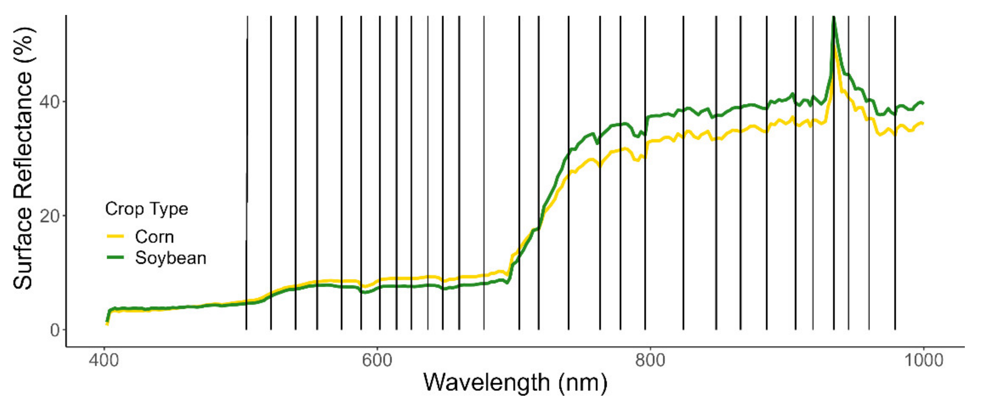
While 15 previously established optimal HNBs were selected for Hyperion, 29 HNBs were selected from DESIS data used in this study within the range of 500–1000 nm. The bands in the 400 to 500 nm region were discarded because many of the reflectance values were negative or zero. The centers of the selected bands were: 504, 522, 540, 556, 574, 588, 602, 614, 625, 637, 648, 660, 678, 704, 718, 740, 763, 778, 796, 824, 848, 866, 885, 906, 919, 934, 945, 960, and 979 nm (Figure 2, Table 4). We used the optimal DESIS and Hyperion bands to classify crop types using various machine learning classification algorithms; their performance is described below.

3.2. Classification Results

Hyperion classifications were run separately for each year (2010, a wet year; 2012, a normal year; and 2013, a dry year in the study area). Results for separate years are available in Supplementary Materials (Tables S1–S116). However, for clarity we have presented results averaged across all 3 years. A summary of sample sizes across all 3 years for Hyperion analyses is shown in Table 5, along with sample sizes for DESIS analysis for 2019, a wet year.
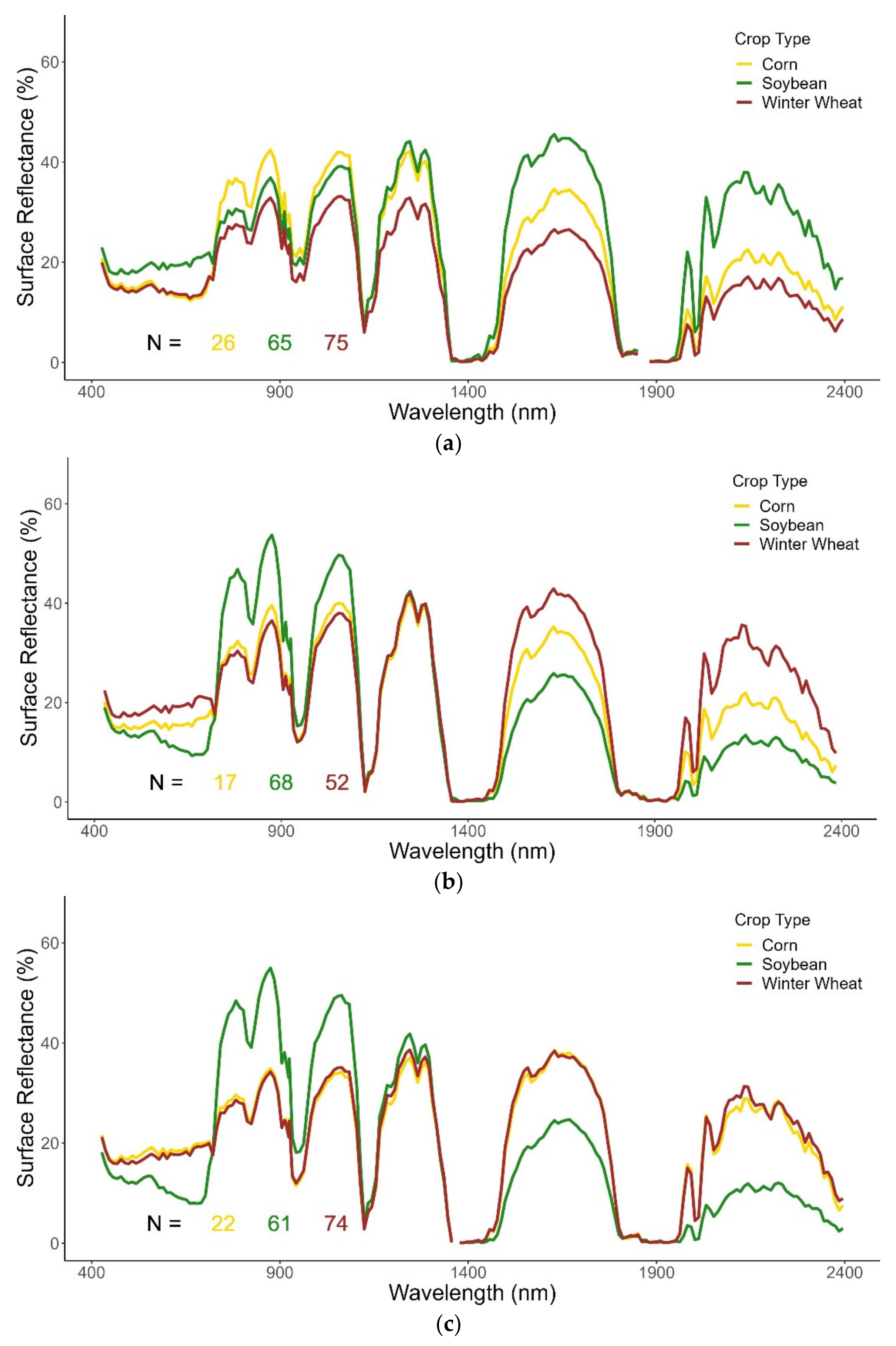
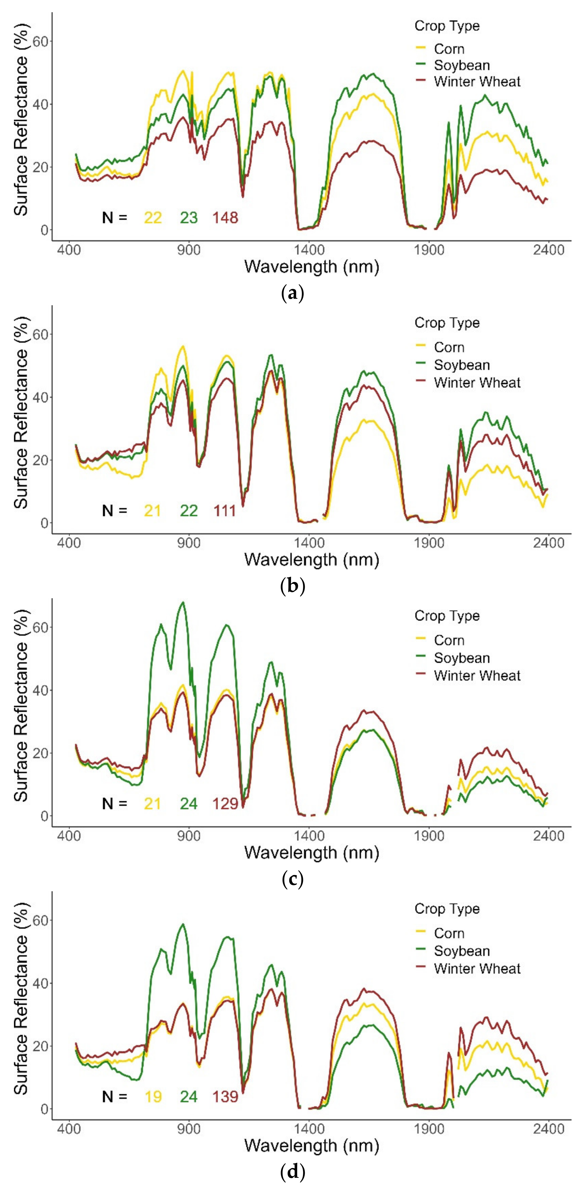
With Hyperion data, crop spectral profiles substantially changed over time, and these changes varied by crop type (Figure 3, Figure 4 and Figure 5). For example, in Hyperion June 2010 data, soybean crops were in early growth stages and had spectra that were highly reflective in the visible (VIS) and shortwave infrared (SWIR) bands, whereas vigorously growing vegetative (i.e., growth and development of non-reproductive structures) stages of corn had higher reflectivity in the near-infrared (NIR) (Figure 3a). However, by August (Figure 3b), vigorously growing soybean had greater absorption in the VIS and greater reflectivity in NIR relative to senescing corn crops.
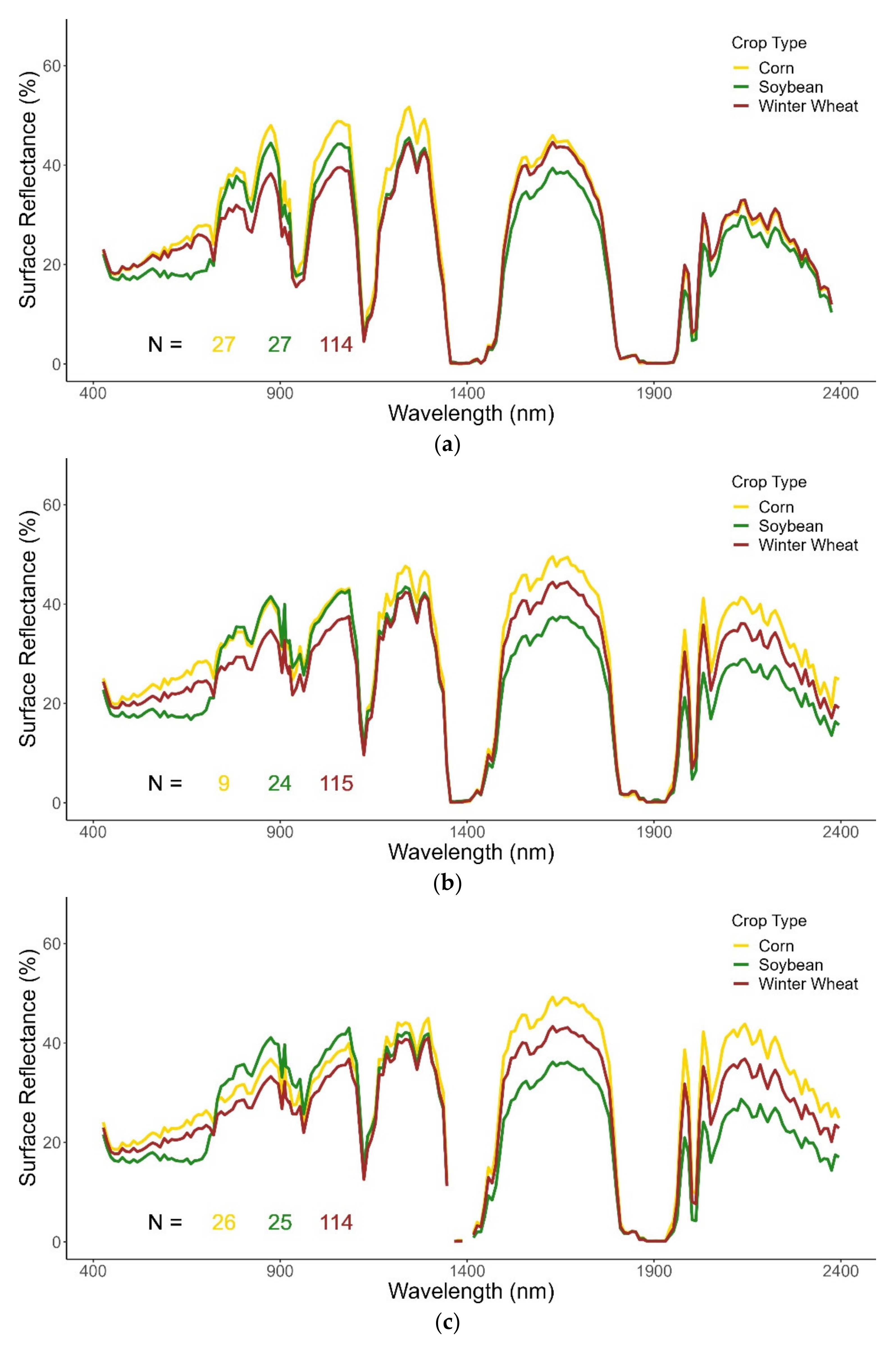
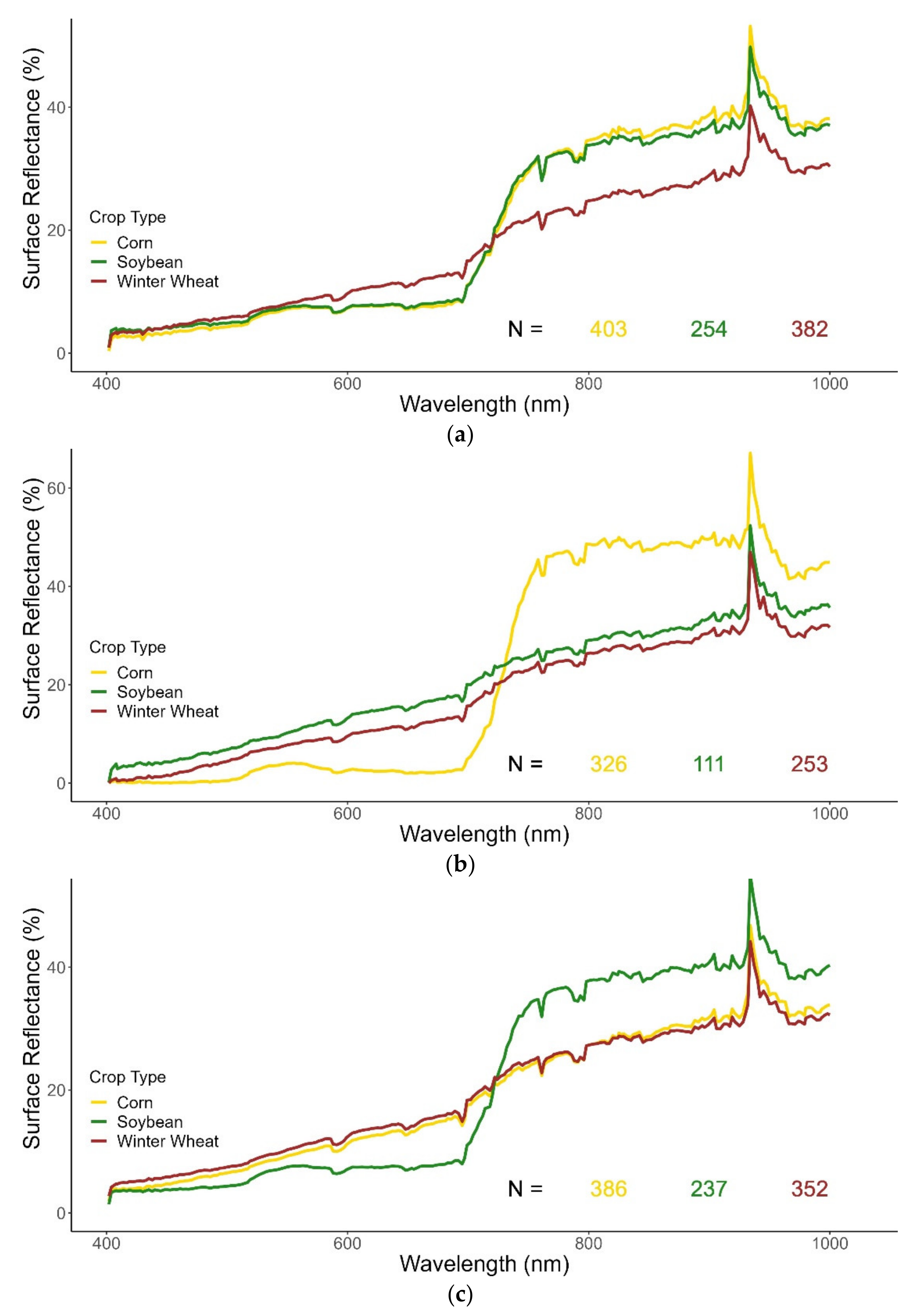
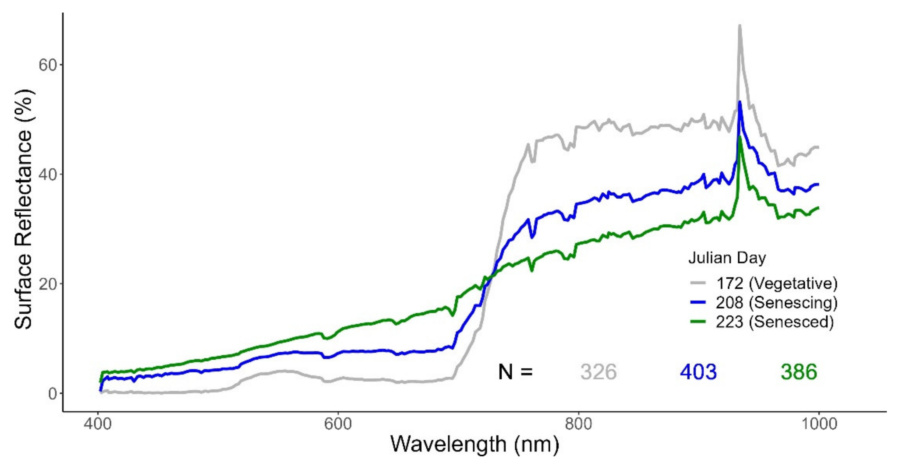
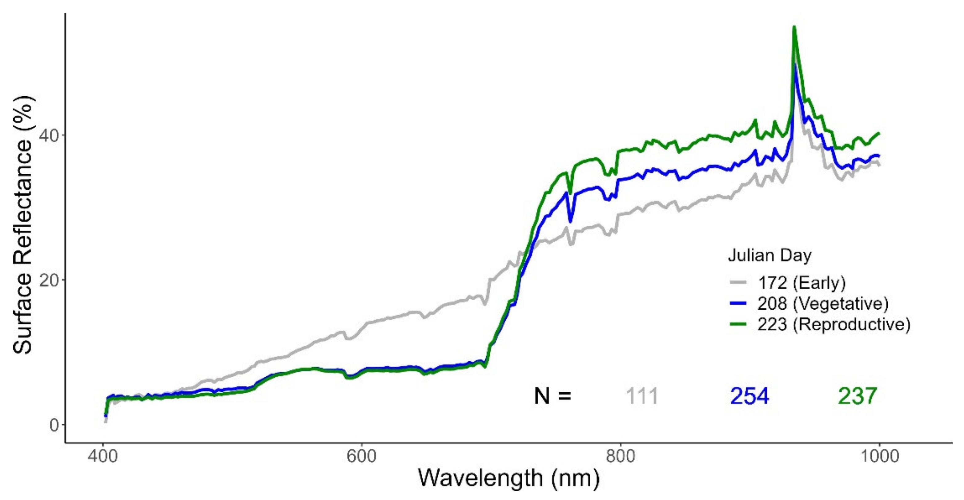
DESIS spectral profiles also varied with crop type and growth stage (Figure 6, Figure 7 and Figure 8). Corn was in the vegetative growth stage on JD 172 (21 June 2019), reproductive in early July (when we have no images), initially senescing by JD 208 (27 July 2019), and mostly senesced by JD 223 (11 August 2019) (Figure 7). Soybean reached the early growth stage on JD 172 (21 June 2019), the vegetative stage on JD 208 (27 July 2019), and the reproductive stage by JD 223 (11 August 2019) (Figure 8).
These spectral differences enabled the differentiation of crop types, especially with RF and SVM, as shown in Table 6, Table 7, Table 8, Table 9, Table 10 and Table 11. For EO-1 Hyperion data, the results indicated that SVM provided the best results, closely followed by RF (Table 6, Table 7, Table 8 and Table 9). SVM and RF provided overall accuracies of 66–76% with single date images, 89–98% with double images, and 96–100% with triple images. Relative to RF and SVM, the NB and WXB algorithms provided much lower accuracies. Across crop type, the RF and SVM classifiers provided 82–100% producer’s accuracies (except for one instance with 64%) and 82–100% user’s accuracies with two or three image dates (Table 6 and Table 7). Again, the NB and WXM accuracies were lower (Table 8 and Table 9). Additionally, the best results were obtained with images later in the growing season (August or September) and/or when two later season images (August and September) were combined, or a later season image (August or September) was combined with an earlier season image (July or June). For Hyperion, later season images when the crop canopy cover was closer to 100% and crops were in vegetative or reproductive growth stages were the best.
As with Hyperion images, DESIS results indicated that RF and SVM provided the best results with overall accuracies of 62–85% as opposed to 34–80% with NB and WXM (Table 10). Also like with Hyperion, the double images yielded higher accuracies than single images. For example, RF single image accuracies of 68–80% were slightly lower than double image accuracies of 67–83%. Similarly, SVM single image accuracies of 62–70% were slightly lower than double image accuracies of 67–85%. However, these improvements going from single to double images were substantially smaller with DESIS images than with Hyperion images. In fact, producer’s and user’s accuracies for winter wheat decreased when using double images (Table 11). Due to the distinct differences in the phenological growth stages of the crops in the June DESIS image, it yielded the highest single image accuracies rather than later in the season. The highest double image accuracies were most often from using one early (June) and one late (August) image (Table 10 and Table 11).
More detailed results are included in the Supplementary Materials, which contain confusion matrices and associated calculations of producer’s, user’s, and overall accuracies. From these matrices, the user can see when crop types were classified correctly and incorrectly. For example, Table S119 shows Random Forest results for the August DESIS imagery data. Out of 129 corn samples, 110 were classified correctly for a producer’s accuracy of 85%. Out of the other 19 misclassified samples, 5 were classified as winter wheat, 6 as other-crop, and 8 as non-crop. Similar error matrices are available in Supplementary Materials for other years, months, sensors, and algorithms (Tables S1–S144).
In addition, to ensure robustness of these classification models, we generated five different training subsets with DESIS data and ran RF and SVM algorithms for each single and double image combination. Overall accuracies were similar across training subsets, with most standard deviations less than 3, and none greater than 5 (see Supplementary Materials Tables S145 and S146).

4. Discussion

Use of selected HS narrowbands reduces data volume, making analysis more efficient and faster. Previous research [3] has found 15 unique and informative Hyperion bands best for agricultural study. However, narrower DESIS bands reveal more spectral features than smoother Hyperion spectral profiles (Figure 3, Figure 4, Figure 5, Figure 6, Figure 7 and Figure 8). As a result, 29 out of 235 DESIS narrowbands (about 12%) were selected as opposed to 15 out of 242 Hyperion narrowbands (about 6%).
Figure 2 shows the band centers of the 29 DESIS narrowbands, which correspond to sudden steep peaks or troughs representing specific crop biophysical or biochemical crop parameters. Several bands in the 400–500 nm region have been used for estimating nitrogen and pigment content, crop biomass and yield, and light use efficiency (LUE); they have also been used to detect weeds and plant stress [3,12,21,86,87,89,90,92]. However, these bands were discarded in DESIS imagery because many of the values were negative or zero, perhaps due to over-correction during the removal of atmospheric effects (standard Level 2a data provided by Teledyne).
Bands selected in this study from 500 to 1000 nm are listed in Table 4, along with similar bands (within 5 nm) used in other studies for various applications [3,12,21,86,87,88,89,90,91,92,93]. These applications include estimation of various plant biophysical and biochemical characteristics like crop biomass and yield, LUE, Leaf Area Index (LAI), nitrogen and pigment content, and moisture. The bands have also been used to detect plant stress, plant disease, and presence of weeds. Additionally, they have been used to classify crop types, crop growth stages, and land use and land cover (LULC) classes. Many of these DESIS optimal bands are similar (within 10 nm) to Hyperion narrowbands: 522 nm (vs. 529 nm for Hyperion), 678 (vs. 681), 718 (vs. 722), 796 (vs. 803), 848 (vs. 844), and 919 (vs. 923). Ultimately, 15 of the 242 Hyperion bands and 29 out of 235 DESIS bands were used for agricultural crop classification. Further studies using different band selection methods (see [94] for examples) may reveal additional important bands.
For Hyperion classification results, Kappa coefficients ranged from 0.28 to 1 with an average of 0.77 (see Supplementary Materials Tables S141–S143). Similarly, for DESIS classifications, Kappa coefficients ranged from 0.51 to 0.77 with an average of 0.64 (see Supplementary Materials Table S144). These high Kappa values indicate the classification results are not due to chance, but to the algorithms effectively classifying crop types, especially when using two or three images throughout a growing season.
All algorithms yielded lower accuracies from DESIS data than from Hyperion data, likely due to its shorter spectral range (Table 1), which does not include information in the SWIR region. Several studies have successfully used RF [95,96,97] and SVM [96,97,98,99,100] for classification of Hyperion data. A few studies have also used NB [98] with Hyperion. However, this is the first study that used WXM with hyperspectral data. Researchers have also successfully used RF [101,102,103] and SVM [101,103] to classify hyperspectral data like APEX and HySPEX. However, this study is among the first to use these algorithms for DESIS classification because DESIS data have become available only recently. We recommend further classification of hyperspectral data should use RF, SVM, and deep learning algorithms such as neural nets. Deep learning (see [104,105,106,107,108] for examples) could yield higher classification accuracies with DESIS data than would traditional machine learning algorithms like those used here.
Deep learning tools are now available in cloud-computing platforms, such as TensorFlow in GEE and PyTorch in Amazon Web Services. When imagery is already available on the cloud-computing platform (e.g., through the platform’s data catalog), as is the case with Hyperion data, many analyses can be done within the Cloud. However, DESIS images are not currently available in GEE’s data catalog. Additionally, as of now, cloud-computing platforms still lack some of the functionality available through proprietary software like ArcMap (e.g., georeferencing). This limitation is particularly challenging for hyperspectral images, which often need more specialized processing than do multispectral data. Nevertheless, DESIS has the potential to provide valuable detailed spectral information that may prove more advantageous with a more comprehensive study across multiple crops, growing conditions, and growth stages.
This study contributes to the existing knowledge base in several novel ways. First, it is currently one of few papers using DESIS data that have the high spectral resolution of 2.55 nm from 400 to 1000 nm, recording data in 235 bands. This unto itself provides several distinct characteristics at specific portions of the spectrum that helps model and map subtle features in plant biophysical and biochemical characteristics (Figure 2 and Table 4). Second, comparison of fine spectral resolution (2.55 nm) DESIS hyperspectral data with another hyperspectral sensor (Hyperion) with significantly coarser spectral resolution of 10 nm provides an interesting study of two generational spaceborne hyperspectral sensors. Third, in an age of evolving high spectral and spatial resolution sensors, development of spectral libraries from multiple sensors becomes critical. In this respect, we have used two generations of hyperspectral sensors to develop spectral libraries of three leading world crops grown in the study area. Fourth, we are currently in an age of machine learning on the Cloud. This study was conducted on GEE using four distinct ML algorithms and adds to evolving literature on optimal machine learning algorithms for agricultural research.

5. Conclusions

In this study, we first developed Hyperion and DESIS hyperspectral libraries of three leading world crops (corn, soybean, and winter wheat) in the study area over Ponca City, Oklahoma. Within- and across-year variability was represented to make the libraries more robust and applicable for training crop models. Second, we established 29 optimal DESIS bands, several of which were like the 15 previously determined Hyperion narrowbands used to study agricultural crops. Lastly, we found agricultural crop types were best classified by the Random Forest (RF) and Support Vector Machine (SVM) supervised classifiers using two generations of hyperspectral narrowband data: new generation DESIS and old-generation Hyperion. The performances of the supervised classification algorithm Naive Bayes (NB) and the unsupervised clustering algorithm WekaXMeans (WXM) were substantially inferior to the SVM and RF for both Hyperion and DESIS hyperspectral sensors. Classification accuracies (overall, producer’s and user’s) increased with the number of images, especially with Hyperion images. The image combinations of late season images (August or September) with early season images (July or June) returned the best results for both sensors. Twenty-nine out of 235 DESIS narrowbands were selected (Table 4) for studying agricultural crops. DESIS images yielded lower classification accuracies relative to Hyperion, probably due to its shorter spectral range (400–1000 nm for DESIS versus 400–2500 nm for Hyperion) that does not include information in the Shortwave Infrared region. We conclude that advances in machine learning, such as through neural nets, will be especially important for analysis of hyperspectral data, which consist of many correlated but potentially informative variables for assessing specific biophysical, biochemical, and plant health characteristics necessary for measuring, modeling, mapping, and monitoring crops. Cloud-computing will facilitate hyperspectral data analysis as new tools, algorithms, and datasets are incorporated within the cloud-computing platform. This study contributes in novel ways to the advancement of hyperspectral data analysis by comparing the new generation spaceborne hyperspectral DESIS data with old generation Hyperion data, through classification of agricultural crops using four different machine learning algorithms on Google Earth Engine.

Supplementary Materials

The following are available online at https://www.mdpi.com/article/10.3390/rs13224704/s1, File S1: Supplementary Material for this Journal Article entitled “Classifying Crop Types Using Two Generations of Hyperspectral Sensors (Hyperion and DESIS) with Machine Learning on the Cloud”.

Author Contributions

Conceptualization, P.S.T.; Formal analysis, I.A.; Methodology, I.A. and P.S.T.; Supervision, P.S.T.; Writing—original draft, I.A. and P.S.T. All authors have read and agreed to the published version of the manuscript.

Funding

This study was funded by the USGS National Land Imaging (NLI) and Land Change Science (LCS) programs of the Land Resources Mission Area, the Core Science Systems (CSS) Mission Area, the USGS Mendenhall Postdoctoral Fellowship program, the waterSMART (Sustain and Manage America’s Resources for Tomorrow) project, the NASA MEaSUREs program (grant number NNH13AV82I) through Global Food Security-support Analysis Data (GFSAD) project, and the NASA HyspIRI (Hyperspectral Infrared Imager currently renamed as Surface Biology and Geology or SBG) mission (NNH10ZDA001N-HYSPIRI). We also appreciate hyperspectral imagery made available through USGS, NASA, and Teledyne Brown Engineering. The use of trade, product, or firm names is for descriptive purposes only and does not constitute endorsement by the U.S. Government.

Data Availability Statement

Several spectral libraries in GHISA (Global Hyperspectral Imaging Spectral-libraries of Agricultural crops) are available through the NASA and USGS LP DAAC (Land Processes Distributed Active Archive Center: https://lpdaac.usgs.gov/ (accessed on 10 September 2021)). Further information on GHISA can be found at the project website (www.usgs.gov/WGSC/GHISA (accessed on 10 September 2021)). For future releases of GHISA data, including those analyzed in this paper, look for updates at www.usgs.gov/WGSC/GHISA (accessed on 10 September 2021) and https://lpdaac.usgs.gov/ (accessed on 10 September 2021).

Acknowledgments

The authors thank internal and external reviewers for their insights, which helped improve the manuscript.

Conflicts of Interest

The authors declare no conflict of interest.

References

  1. Lu, B.; Dao, P.; Liu, J.; He, Y.; Shang, J. Recent advances of hyperspectral imaging technology and applications in agriculture. Remote Sens. 2020, 12, 2659. [Google Scholar] [CrossRef]
  2. Aneece, I.P.; Thenkabail, P.S.; Lyon, J.G.; Huete, A.; Slonecker, T. Spaceborne hyperspectral EO-1 Hyperion data pre-processing: Methods, approaches, and algorithms. In Fundamentals, Sensor Systems, Spectral Libraries, and Data Mining for Vegetation; Taylor and Francis Inc.\CRC Press: Boca Raton, FL, USA, 2018. [Google Scholar]
  3. Aneece, I.; Thenkabail, P. Accuracies Achieved in classifying five leading world crop types and their growth stages using optimal earth Observing-1 Hyperion hyperspectral Narrowbands on Google earth engine. Remote Sens. 2018, 10, 2027. [Google Scholar] [CrossRef] [Green Version]
  4. Kennedy, B.; King, D.; Duffe, J. Comparison of empirical and physical modelling for estimation of biochemical and biophysical vegetation properties: Field scale analysis across an Arctic bioclimatic gradient. Remote Sens. 2020, 12, 3073. [Google Scholar] [CrossRef]
  5. Thenkabail, P.S.; Aneece, I.; Teluguntla, P.; Oliphant, A. Hyperspectral narrowband data propel gigantic leap in the earth remote sensing. Photogramm. Eng. Remote Sens. 2021, 87, 461–467. [Google Scholar] [CrossRef]
  6. Thenkabail, P.; Lyon, G.; Huete, A. Hyperspectral Remote Sensing of Vegetation; Volume I: Fundamentals, Sensor Systems, Spectral Libraries, and Data Mining for Vegetation; Taylor and Francis Inc.\CRC Press: New York, NY, USA, 2018; p. 449. [Google Scholar]
  7. Thenkabail, P.; Lyon, G.; Huete, A. Hyperspectral Remote Sensing of Vegetation; Volume II: Hyperspectral Indices and Image Classifications for Agriculture and Vegetation; Taylor and Francis Inc.\CRC Press: New York, NY, USA, 2018; p. 296. [Google Scholar]
  8. Thenkabail, P.; Lyon, G.; Huete, A. Hyperspectral Remote Sensing of Vegetation; Volume III: Biophysical and Biochemical Characterization and Plant Species Studies; Taylor and Francis Inc.\CRC Press: New York, NY, USA, 2018; p. 348. [Google Scholar]
  9. Thenkabail, P.; Lyon, G.; Huete, A. Hyperspectral Remote Sensing of Vegetation; Volume IV: Advanced Applications in Remote Sensing of Agricultural Crops and Natural Vegetation; Taylor and Francis Inc.\CRC Press: New York, NY, USA, 2018; p. 386. [Google Scholar]
  10. Vali, A.; Comai, S.; Matteucci, M. Deep learning for land use and land cover classification based on hyperspectral and multispectral earth observation data: A review. Remote Sens. 2020, 12, 2495. [Google Scholar] [CrossRef]
  11. Marshall, M.; Thenkabail, P.; Biggs, T.; Post, K. Hyperspectral narrowband and multispectral broadband indices for remote sensing of crop evapotranspiration and its components (transpiration and soil evaporation). Agric. For. Meteorol. 2016, 218–219, 122–134. [Google Scholar] [CrossRef] [Green Version]
  12. Mariotto, I.; Thenkabail, P.S.; Huete, A.; Slonecker, E.T.; Platonov, A. Hyperspectral versus multispectral crop-productivity modeling and type discrimination for the HyspIRI mission. Remote Sens. Environ. 2013, 139, 291–305. [Google Scholar] [CrossRef]
  13. Dennison, P.E.; Qi, Y.; Meerdink, S.K.; Kokaly, R.F.; Thompson, D.R.; Daughtry, C.S.T.; Quemada, M.; Roberts, D.A.; Gader, P.D.; Wetherley, E.B.; et al. Comparison of methods for modeling fractional cover using simulated satellite hyperspectral imager spectra. Remote Sens. 2019, 11, 2072. [Google Scholar] [CrossRef]
  14. Thenkabail, P.; Teluguntla, P.; Xiong, J.; Oliphant, A.; Congalton, R.; Ozdogan, M.; Gumma, M.; Tilton, J.; Giri, C.; Milesi, C.; et al. Global Cropland Extent Product at 30m (GCEP30) Derived Using Landsat Satellite Time-Series Data for the Year 2015 through Multiple Machine Learning Algorithms on Google Earth Engine (GEE) Cloud; United States Geological Survey (USGS): Reston, VA, USA, 2021; Research Paper in Press. [Google Scholar]
  15. Christian, B.; Joshi, N.; Saini, M.; Mehta, N.; Goroshi, S.; Nidamanuri, R.R.; Thenkabail, P.; Desai, A.R.; Krishnayya, N. Seasonal variations in phenology and productivity of a tropical dry deciduous forest from MODIS and Hyperion. Agric. For. Meteorol. 2015, 214–215, 91–105. [Google Scholar] [CrossRef]
  16. Gerhards, M.; Schlerf, M.; Mallick, K.; Udelhoven, T. Challenges and future perspectives of Multi-/Hyperspectral thermal infrared remote sensing for crop Water-Stress detection: A review. Remote Sens. 2019, 11, 1240. [Google Scholar] [CrossRef] [Green Version]
  17. Kwan, C.; Ayhan, B.; Budavari, B.; Lu, Y.; Perez, D.; Li, J.; Bernabe, S.; Plaza, A. Deep Learning for land cover classification using only a few bands. Remote Sens. 2020, 12, 2000. [Google Scholar] [CrossRef]
  18. Lv, W.; Wang, X. Overview of hyperspectral image classification. J. Sens. 2020, 2020, 4817234. [Google Scholar] [CrossRef]
  19. Marshall, M.; Thenkabail, P. Advantage of hyperspectral EO-1 Hyperion over multispectral IKONOS, GeoEye-1, WorldView-2, Landsat ETM+, and MODIS vegetation indices in crop biomass estimation. ISPRS J. Photogramm. Remote Sens. 2015, 108, 205–218. [Google Scholar] [CrossRef] [Green Version]
  20. Marshall, M.; Thenkabail, P.S. Biomass Modeling of four leading world crops using hyperspectral narrowbands in support of HyspIRI mission. Photogramm. Eng. Remote Sens. 2014, 80, 757–772. [Google Scholar] [CrossRef]
  21. Thenkabail, P.; Mariotto, I.; Gumma, M.; Middleton, E.; Landis, D.; Huemmrich, K. Selection of hyperspectral narrowbands (HNBs) and composition of hyperspectral two band vegetation indices (HVIs) for biophysical characterization and discrimination of crop types using field reflectance and Hyperion/ EO-1 data. IEEE J. Sel. Top. Appl. Earth Obs. Remote Sens. 2013, 6, 427–439. [Google Scholar] [CrossRef] [Green Version]
  22. Hoeppner, J.M.; Skidmore, A.K.; Darvishzadeh, R.; Heurich, M.; Chang, H.-C.; Gara, T.W. Mapping Canopy chlorophyll content in a temperate forest using airborne hyperspectral data. Remote Sens. 2020, 12, 3573. [Google Scholar] [CrossRef]
  23. Tsagkatakis, G.; Aidini, A.; Fotiadou, K.; Giannopoulos, M.; Pentari, A.; Tsakalides, P. Survey of Deep-Learning approaches for remote sensing observation enhancement. Sensors 2019, 19, 3929. [Google Scholar] [CrossRef] [Green Version]
  24. Liu, B.; Liu, Z.; Men, S.; Li, Y.; Ding, Z.; He, J.; Zhao, Z. Underwater hyperspectral imaging technology and its applications for detecting and mapping the seafloor: A review. Sensors 2020, 20, 4962. [Google Scholar] [CrossRef]
  25. Herrmann, I.; Berger, K. Remote and proximal assessment of plant traits. Remote Sens. 2021, 13, 1893. [Google Scholar] [CrossRef]
  26. Xiong, J.; Thenkabail, P.S.; Tilton, J.C.; Gumma, M.K.; Teluguntla, P.; Oliphant, A.; Congalton, R.G.; Yadav, K.; Gorelick, N. Nominal 30-m cropland extent map of continental africa by integrating pixel-based and object-based algorithms using Sentinel-2 and Landsat-8 data on google earth engine. Remote Sens. 2017, 9, 1065. [Google Scholar] [CrossRef] [Green Version]
  27. Brovelli, M.A.; Sun, Y.; Yordanov, V. Monitoring forest change in the amazon using Multi-Temporal remote sensing data and machine learning classification on google earth engine. ISPRS Int. J. Geo-Inf. 2020, 9, 580. [Google Scholar] [CrossRef]
  28. Tian, H.; Pei, J.; Huang, J.; Li, X.; Wang, J.; Zhou, B.; Qin, Y.; Wang, L. Garlic and winter wheat identification based on active and passive satellite imagery and the google earth engine in northern china. Remote Sens. 2020, 12, 3539. [Google Scholar] [CrossRef]
  29. Amani, M.; Kakooei, M.; Moghimi, A.; Ghorbanian, A.; Ranjgar, B.; Mahdavi, S.; Davidson, A.; Fisette, T.; Rollin, P.; Brisco, B.; et al. Application of google earth engine cloud computing platform, sentinel imagery, and neural networks for crop mapping in Canada. Remote Sens. 2020, 12, 3561. [Google Scholar] [CrossRef]
  30. Naboureh, A.; Ebrahimy, H.; Azadbakht, M.; Bian, J.; Amani, M. RUESVMs: An ensemble method to handle the class imbalance problem in land cover mapping using Google Earth Engine. Remote Sens. 2020, 12, 3484. [Google Scholar] [CrossRef]
  31. Sankey, T.; Belmonte, A.; Massey, R.; Leonard, J. Regional-Scale forest restoration effects on ecosystem resiliency to drought: A synthesis of vegetation and moisture trends on Google Earth Engine. Remote Sens. Ecol. Conserv. 2021, 7, 259–274. [Google Scholar] [CrossRef]
  32. Teluguntla, P.; Thenkabail, P.; Xiong, J.; Gumma, M.; Giri, C.; Milesi, C.; Ozdogan, M.; Congalton, R.; Tilton, J.; Sankey, T.; et al. Global food security support analysis data at nominal 1 km (GFSAD1km) derived from remote sensing in support of food security in the Twenty-First century: Current achievements and future possibilities, Chapter 6. In Remote Sensing Handbook Volume II: Land Resources Monitoring, Modeling, and Mapping with Remote Sensing; CRC Press: Boca Raton, FL, USA, 2015; pp. 131–160. [Google Scholar]
  33. Teluguntla, P.; Thenkabail, P.S.; Xiong, J.; Gumma, M.K.; Congalton, R.G.; Oliphant, A.; Poehnelt, J.; Yadav, K.; Rao, M.; Massey, R. Spectral matching techniques (SMTs) and automated cropland classification algorithms (ACCAs) for mapping croplands of Australia using MODIS 250-m time-series (2000–2015) data. Int. J. Digit. Earth 2017, 10, 944–977. [Google Scholar] [CrossRef] [Green Version]
  34. Paoletti, M.E.; Haut, J.M.; Plaza, J.; Plaza, A. Deep learning classifiers for hyperspectral imaging: A review. ISPRS J. Photogramm. Remote Sens. 2019, 158, 279–317. [Google Scholar] [CrossRef]
  35. Panda, S.; Rao, M.; Thenkabail, P.; Fitzerald, J. Remote sensing systems–platforms and sensors: Aerial, satellites, UAVs, optical, radar, and LiDAR, Chapter 1. In Remote Sensing Handbook, Volume I: Remotely Sensed Data Characterization, Classification, and Accuracies; USGS: Boca Raton, FL, USA, 2015; pp. 3–60. [Google Scholar]
  36. Cogliati, S.; Sarti, F.; Chiarantini, L.; Cosi, M.; Lorusso, R.; Lopinto, E.; Miglietta, F.; Genesio, L.; Guanter, L.; Damm, A.; et al. The PRISMA imaging spectroscopy mission: Overview and first performance analysis. Remote Sens. Environ. 2021, 262, 112499. [Google Scholar] [CrossRef]
  37. Cawse-Nicholson, K.; Townsend, P.; Schimel, D.; Assiri, A.; Blake, P.; Buongiorno, M.; Campbell, P.; Carmon, N.; Casey, K.; Correa-Pabón, R.; et al. NASA’s surface biology and geology designated observable: A perspective on surface imaging algorithms. Remote Sens. Environ. 2021, 257, 2–26. [Google Scholar] [CrossRef]
  38. Eckardt, A.; Horack, J.; Lehmann, F.; Krutz, D.; Drescher, J.; Whorton, M.; Soutullo, M. DESIS (DLR earth sensing imaging spectrometer for the ISS-MUSES platform). In Proceedings of the 2015 IEEE International Geoscience and Remote Sensing Symposium (IGARSS), Milan, Italy, 26–31 July 2015; pp. 1457–1459. [Google Scholar]
  39. Krutz, D.; Müller, R.; Knodt, U.; Günther, B.; Walter, I.; Sebastian, I.; Säuberlich, T.; Reulke, R.; Carmona, E.; Eckardt, A.; et al. The instrument design of the DLR Earth Sensing Imaging Spectrometer (DESIS). Sensors 2019, 19, 1622. [Google Scholar] [CrossRef] [PubMed] [Green Version]
  40. Ren, Z.; Sun, L.; Zhai, Q. Improved k-means and spectral matching for hyperspectral mineral mapping. Int. J. Appl. Earth Obs. Geoinf. 2020, 91, 102154. [Google Scholar] [CrossRef]
  41. Laporte-Fauret, Q.; Lubac, B.; Castelle, B.; Michalet, R.; Marieu, V.; Bombrun, L.; Launeau, P.; Giraud, M.; Normandin, C.; Rosebery, D. Classification of atlantic coastal sand dune vegetation using in situ, UAV, and airborne hyperspectral data. Remote Sens. 2020, 12, 2222. [Google Scholar] [CrossRef]
  42. Liu, Y.; Lyu, S.; Hou, M.; Gao, Z.; Wang, W.; Zhou, X. A novel spectral matching approach for pigment: Spectral subsection identification considering ion absorption characteristics. Remote Sens. 2020, 12, 3415. [Google Scholar] [CrossRef]
  43. Dai, J.; Roberts, D.A.; Stow, D.A.; An, L.; Hall, S.J.; Yabiku, S.T.; Kyriakidis, P.C. Mapping understory invasive plant species with field and remotely sensed data in Chitwan, Nepal. Remote Sens. Environ. 2020, 250, 112037. [Google Scholar] [CrossRef]
  44. Mariotto, I.; Thenkabail, P.; Aneece, I. Global hyperspectral imaging Spectral-library of agricultural crops (GHISA) area of study: Central Asia. In Algorithm Theoretical Basis Document (ATBD); NASA Land Processes Distributed Active Archive Center (LP DAAC): Sioux Falls, SD, USA, 2020; p. 28. [Google Scholar]
  45. Mariotto, I.; Thenkabail, P.; Aneece, I. Global Hyperspectral Imaging Spectral-Library of Agricultural Crops (GHISA) Area of Study: Central Asia: User Guide; NASA Land Processes Distributed Active Archive Center (LP DAAC): Sioux Falls, SD, USA, 2020; p. 7. [Google Scholar]
  46. Aneece, I.; Thenkabail, P.; Aneece, I. Global hyperspectral imaging Spectral-library of agricultural crops (GHISA) area of study: Central Asia. In Algorithm Theoretical Basis Document (ATBD); NASA Land Processes Distributed Active Archive Center (LP DAAC): Sioux Falls, SD, USA, 2019; p. 25. [Google Scholar]
  47. Aneece, I.; Thenkabail, P. Global Hyperspectral Imaging Spectral-Library of Agricultural Crops (GHISA) for the Conterminous United States (CONUS): User Guide; NASA Land Processes Distributed Active Archive Center (LP DAAC): Sioux Falls, SD, USA, 2019; p. 7. [Google Scholar]
  48. Mesonet. January 28–30, 2002: Oklahoma Ice Storm; Oklahoma Climate: Long Term Averages and Extremes. Oklahoma Climatalogical Survey. Available online: http://climate.ok.gov/index.php/climate (accessed on 15 September 2021).
  49. Mesonet. Available online: http://www.mesonet.org/index.php/site/sites/station_names_map# (accessed on 15 September 2021).
  50. USDA. Cropscape-Cropland Data Layer. 2018. Available online: https://nassgeodata.gmu.edu/CropScape/ (accessed on 10 September 2021).
  51. NASS. USDA Crop Production 2017 Summary: January 2018; Technical Report; United States Department of Agriculture, National Agricultural Statistics Service: Washington, DC, USA, 2018. [Google Scholar]
  52. NASS. USDA CropScape and Cropland Data Layer-Metadata; Technical Report; United States Department of Agriculture, National Agricultural Statistics Service: Washington, DC, USA, 2018. [Google Scholar]
  53. Zhang, C.; Di, L.; Hao, P.; Yang, Z.; Lin, L.; Zhao, H.; Guo, L. Rapid in-season mapping of corn and soybeans using machine-learned trusted pixels from Cropland Data Layer. Int. J. Appl. Earth Obs. Geoinf. 2021, 102, 102374. [Google Scholar] [CrossRef]
  54. Boryan, C.; Yang, Z. Integration of the Cropland Data Layer based automatic stratification method into the traditional area frame construction process. Surv. Res. Methods 2021, 11, 289–306. [Google Scholar]
  55. Hao, P.; Wang, L.; Wang, L.; Zhan, Y.; Niu, Z.; Wu, M. Crop classification using crop knowledge of the previous-year: Case study in Southwest Kansas, USA. Eur. J. Remote Sens. 2016, 49, 1061–1077. [Google Scholar] [CrossRef] [Green Version]
  56. Zhong, L.; Gong, P.; Biging, G.S. Efficient corn and soybean mapping with temporal extendability: A multi-year experiment using Landsat imagery. Remote Sens. Environ. 2014, 140, 1–13. [Google Scholar] [CrossRef]
  57. Lark, T.; Schelly, I.; Gibbs, H. Accuracy, bias, and improvements in mapping crops and cropland across the United States using the USDA Cropland Data Layer. Remote Sens. 2021, 13, 968. [Google Scholar] [CrossRef]
  58. Sacks, W.J.; Deryng, D.; Foley, J.A.; Ramankutty, N. Crop planting dates: An analysis of global patterns. Glob. Ecol. Biogeogr. 2010, 19, 607–620. [Google Scholar] [CrossRef]
  59. USGS. USGS Global food Security-Support Analysis Data at 30 m (GFSAD30). 2015. Available online: https://www.usgs.gov/centers/wgsc/science/global-food-security-support-analysis-data-30-m-gfsad?qt-science_center_objects=0#qt-science_center_objects (accessed on 1 January 2021).
  60. Yadav, K.; Congalton, R.G. Accuracy assessment of global food security-support analysis data (GFSAD) cropland extent maps produced at three different spatial resolutions. Remote Sens. 2018, 10, 1800. [Google Scholar] [CrossRef] [Green Version]
  61. Massey, R.; Sankey, T.T.; Congalton, R.G.; Yadav, K.; Thenkabail, P.S.; Ozdogan, M.; Meador, A.S. MODIS phenology-derived, multi-year distribution of conterminous U.S. crop types. Remote Sens. Environ. 2017, 198, 490–503. [Google Scholar] [CrossRef]
  62. Thenkabail, P.S.; Enclona, E.A.; Ashton, M.S.; Legg, C.; De Dieu, M.J. Hyperion, IKONOS, ALI, and ETM+ sensors in the study of African rainforests. Remote Sens. Environ. 2004, 90, 23–43. [Google Scholar] [CrossRef]
  63. Datt, B.; McVicar, T.; Van Niel, T.; Jupp, D.; Pearlman, J. Preprocessing eo-1 hyperion hyperspectral data to support the application of agricultural indexes. IEEE Trans. Geosci. Remote Sens. 2003, 41, 1246–1259. [Google Scholar] [CrossRef] [Green Version]
  64. Suarez, L.A.; Apan, A.; Werth, J. Detection of phenoxy herbicide dosage in cotton crops through the analysis of hyperspectral data. Int. J. Remote Sens. 2017, 38, 6528–6553. [Google Scholar] [CrossRef]
  65. Nugent, P.W.; Shaw, J.A.; Jha, P.; Scherrer, B.; Donelick, A.; Kumar, V. Discrimination of herbicide-resistant kochia with hyperspectral imaging. J. Appl. Remote Sens. 2018, 12, 016037. [Google Scholar] [CrossRef] [Green Version]
  66. Feng, H.; Jiang, N.; Huang, C.; Fang, W.; Yang, W.; Chen, G.; Xiong, L.; Liu, Q. A hyperspectral imaging system for an accurate prediction of the above-ground biomass of individual rice plants. Rev. Sci. Instrum. 2013, 84, 095107. [Google Scholar] [CrossRef] [PubMed]
  67. Liu, J.; Miller, J.; Pattey, E.; Haboudane, D.; Strachan, I.; Hinther, M. Monitoring crop biomass accumulation using multi-temporal hyper-spectral remote sensing data. IEEE Int. Geosci. Remote Sens. Symp. 2004, 3, 1637–1640. [Google Scholar]
  68. Mutanga, O.; Skidmore, A.K. Narrow band vegetation indices overcome the saturation problem in biomass estimation. Int. J. Remote Sens. 2004, 25, 3999–4014. [Google Scholar] [CrossRef]
  69. Ngie, A. Estimation of maize nitrate concentrations using EO-1 data and a non-linear regression model. ISPRS Int. Arch. Photogramm. Remote Sens. Spat. Inf. Sci. 2020, XLII-3/W11, 109–116. [Google Scholar] [CrossRef] [Green Version]
  70. Jacon, A.; Galvao, L.; Dalagnol, R.; Santos, J. Aboveground biomass estimates over Brazilian savannas using hyperspectral metrics and machine learning models: Experiences with Hyperion/EO-1. GISci. Remote Sens. 2021, 58, 1112–1129. [Google Scholar] [CrossRef]
  71. Moharana, S. Hyperspectral Remote Sensing of Rice Agriculture for Field Scale Variability Mapping. Ph.D. Thesis, Indian Institute of Technology Guwahati, Dept. of Civil Engineering, Guwahati, India, December 2018. [Google Scholar]
  72. Omran, E. Remote estimation of vegetation parameters using narrow band sensor for precision agriculture in arid environment. Egypt. J. Soil Sci. 2018, 58, 73–92. [Google Scholar] [CrossRef] [Green Version]
  73. Ramesh, H.; Soorya, P.P. Application of EO-1 hyperion data for mapping and discrimination of agricultural crops. In Pond Ecosystems of the Indian Sundarbans; Springer: New York, NY, USA, 2018; Volume 81, pp. 401–421. [Google Scholar]
  74. Thenkabail, P.S.; Smith, R.B.; De Pauw, E. Hyperspectral vegetation indices and their relationships with agricultural crop characteristics. Remote Sens. Environ. 2000, 71, 158–182. [Google Scholar] [CrossRef]
  75. Tyralis, H.; Papacharalampous, G.; Langousis, A. A brief review of random forests for water scientists and practitioners and their recent history in water resources. Water 2020, 11, 910. [Google Scholar] [CrossRef] [Green Version]
  76. Chen, W.; Li, Y.; Tsangaratos, P.; Shahabi, H.; Ilia, I.; Xue, W.; Bian, H. Groundwater spring potential mapping using artificial intelligence approach based on kernel logistic regression, random forest, and alternating decision tree models. Appl. Sci. 2020, 10, 425. [Google Scholar] [CrossRef] [Green Version]
  77. Sheykhmousa, M.; Mahdianpari, M.; Ghanbari, H.; Mohammadimanesh, F.; Ghamisi, P.; Homayouni, S. Support vector machine versus random forest for remote sensing image classification: A meta-analysis and systematic review. IEEE J. Sel. Top. Appl. Earth Obs. Remote Sens. 2020, 13, 6308–6325. [Google Scholar] [CrossRef]
  78. Wu, Y.; Zhang, X. Object-Based tree species classification using airborne hyperspectral images and LiDAR data. Forests 2019, 11, 32. [Google Scholar] [CrossRef] [Green Version]
  79. Abdi, A.M. Land cover and land use classification performance of machine learning algorithms in a boreal landscape using Sentinel-2 data. GISci. Remote Sens. 2020, 57, 1–20. [Google Scholar] [CrossRef] [Green Version]
  80. Cubranic, D.; Murphy, G. Automatic bug triage using text categorization. In Proceedings of the Sixteenth International Conference on Software Engineering & Knowledge Engineering; Citeseer: State College, PA, USA, 2004; pp. 92–97. [Google Scholar]
  81. Mori, T. Superposed naive bayes for accurate and interpretable prediction. In Proceedings of the 2015 IEEE 14th International Conference on Machine Learning and Applications (ICMLA), Miami, FL, USA, 9–11 December 2015; pp. 1228–1233. [Google Scholar]
  82. Xuan, J.; Jiang, H.; Ren, Z.; Yan, J.; Luo, Z. Automatic bug triage using semi-supervised text classification. arXiv 2017, arXiv:1704.04769, 6. [Google Scholar]
  83. Pelleg, D.; Moore, A. X-means: Extending K-means with efficient estimation of the number of clusters. InIcml 2000, 1, 727–734. [Google Scholar]
  84. Pelleg, D.; Moore, A. Accelerating exact k-means algorithms with geometric reasoning. In Proceedings of the Fifth ACM SIGKDD International Conference on Knowledge Discovery and Data Mining; Carnegie Melon University: Pittsburgh, PA, USA, 1999; pp. 277–281. [Google Scholar]
  85. Laloe, T.; Servien, R. The X-Alter algorithm: A parameter-free method to perform unsupervised clustering. J. Mod. Appl. Stat. Methods 2013, 12, 90–102. [Google Scholar] [CrossRef]
  86. Zhang, W.; Li, X.; Zhao, L. Band priority index: A feature selection framework for hyperspectral imagery. Remote Sens. 2018, 10, 1095. [Google Scholar] [CrossRef] [Green Version]
  87. Ren, J.; Wang, R.; Liu, G.; Feng, R.; Wang, Y.; Wu, W. Partitioned relief-F method for dimensionality reduction of hyperspectral images. Remote Sens. 2020, 12, 1104. [Google Scholar] [CrossRef] [Green Version]
  88. Chen, Z.; Jia, K.; Xiao, C.; Wei, D.; Zhao, X.; Lan, J.; Wei, X.; Yao, Y.; Wang, B.; Sun, Y.; et al. Leaf area index estimation algorithm for GF-5 hyperspectral data based on different feature selection and machine learning methods. Remote Sens. 2020, 12, 2110. [Google Scholar] [CrossRef]
  89. Deng, X.; Zhu, Z.; Yang, J.; Zheng, Z.; Huang, Z.; Yin, X.; Wei, S.; Lan, Y. Detection of citrus huanglongbing based on multi-input neural network model of UAV hyperspectral remote sensing. Remote Sens. 2020, 12, 2678. [Google Scholar] [CrossRef]
  90. Thenkabail, P.; Gumma, M.; Telaguntla, P.; Mohammed, I. Hyperspectral remote sensing of vegetation and agricultural crops. Photogramm. Eng. Remote Sens. 2014, 80, 697–709. [Google Scholar]
  91. Ma, H.; Zhao, K.; Jin, X.; Ji, J.; Qiu, Z.; Gao, S. Spectral difference analysis and identification of different maturity blueberry fruit based on hyperspectral imaging using spectral index. Int. J. Agric. Biol. Eng. 2019, 12, 134–140. [Google Scholar] [CrossRef] [Green Version]
  92. Mudereri, B.T.; Dube, T.; Niassy, S.; Kimathi, E.; Landmann, T.; Khan, Z.; Abdel-Rahman, E.M. Is it possible to discern Striga weed (Striga hermonthica) infestation levels in maize agro-ecological systems using in-situ spectroscopy? Int. J. Appl. Earth Obs. Geoinf. 2020, 85, 102008. [Google Scholar] [CrossRef]
  93. Salem, S.I.; Higa, H.; Kim, H.; Kobayashi, H.; Oki, K.; Oki, T. Assessment of chlorophyll-a algorithms considering different trophic statuses and optimal bands. Sensors 2017, 17, 1746. [Google Scholar] [CrossRef] [Green Version]
  94. Sun, W.; Du, Q. Hyperspectral band selection: A review. IEEE Geosci. Remote Sens. Mag. 2019, 7, 118–139. [Google Scholar] [CrossRef]
  95. Kattenborn, T.; Maack, J.; Fassnacht, F.; Enßle, F.; Ermert, J.; Koch, B. Mapping forest biomass from space–Fusion of hyperspectral EO1-hyperion data and Tandem-X and WorldView-2 canopy height models. Int. J. Appl. Earth Obs. Geoinf. 2015, 35, 359–367. [Google Scholar] [CrossRef]
  96. Rodriguez-Galiano, V.; Sanchez-Castillo, M.; Chica-Olma, M.; Chica-Rivas, M. Machine learning predictive models for mineral prospectivity: An evaluation of neural networks, random forest, regression trees and support vector machines. Ore Geol. Rev. 2015, 71, 804–818. [Google Scholar] [CrossRef]
  97. Puletti, N.; Camarretta, N.; Corona, P. Evaluating EO1-Hyperion capability for mapping conifer and broadleaved forests. Eur. J. Remote Sens. 2016, 49, 157–169. [Google Scholar] [CrossRef] [Green Version]
  98. Praveen, Y.; Kiranmai, A.; Nikitha, K.; Devi, V. Hyperspectral sensor data fusion at decision level using support vector machine. Int. J. Res. Eng. Technol. 2016, 5, 14–18. [Google Scholar]
  99. Gopinath, G.; Sasidharan, N.; Surendran, U. Landuse classification of hyperspectral data by spectral angle mapper and support vector machine in humid tropical region of India. Earth Sci. Inform. 2020, 13, 633–640. [Google Scholar] [CrossRef]
  100. Lin, Z.; Yan, L. A support vector machine classifier based on a new kernel function model for hyperspectral data. GISci. Remote Sens. 2016, 53, 85–101. [Google Scholar] [CrossRef]
  101. Sabat-Tomala, A.; Raczko, E.; Zagajewski, B. Comparison of support vector machine and random forest algorithms for invasive and expansive species classification using airborne hyperspectral data. Remote Sens. 2020, 12, 516. [Google Scholar] [CrossRef] [Green Version]
  102. Tan, K.; Wang, H.; Chen, L.; Du, Q.; Du, P.; Pan, C. Estimation of the spatial distribution of heavy metal in agricultural soils using airborne hyperspectral imaging and random forest. J. Hazard. Mater. 2020, 382, 120987. [Google Scholar] [CrossRef]
  103. Raczko, E.; Zagajewski, B. Comparison of support vector machine, random forest and neural network classifiers for tree species classification on airborne hyperspectral APEX images. Eur. J. Remote Sens. 2017, 50, 144–154. [Google Scholar] [CrossRef] [Green Version]
  104. Kamilaris, A.; Prenafeta-Boldú, F.X. Deep learning in agriculture: A survey. Comput. Electron. Agric. 2018, 147, 70–90. [Google Scholar] [CrossRef] [Green Version]
  105. Liakos, K.G.; Busato, P.; Moshou, D.; Pearson, S.; Bochtis, D. Machine learning in agriculture: A review. Sensors 2018, 18, 2674. [Google Scholar] [CrossRef] [Green Version]
  106. Ghamisi, P.; Plaza, J.; Chen, Y.; Li, J.; Plaza, A. Advanced supervised classifiers for hyperspectral images: A review. IEEE Geosci. Remote Sens. Mag. 2017, 5, 1–23. [Google Scholar]
  107. Audebert, N.; Le Saux, B.; Lefèvre, S. Deep learning for classification of hyperspectral data: A comparative review. IEEE Geosci. Remote Sens. Mag. 2019, 7, 159–173. [Google Scholar] [CrossRef] [Green Version]
  108. Li, S.; Song, W.; Fang, L.; Chen, Y.; Ghamisi, P.; Benediktsson, J. Deep learning for hyperspectral image classification: An overview. IEEE Trans. Geosci. Remote Sens. 2019, 57, 6690–6709. [Google Scholar] [CrossRef] [Green Version]
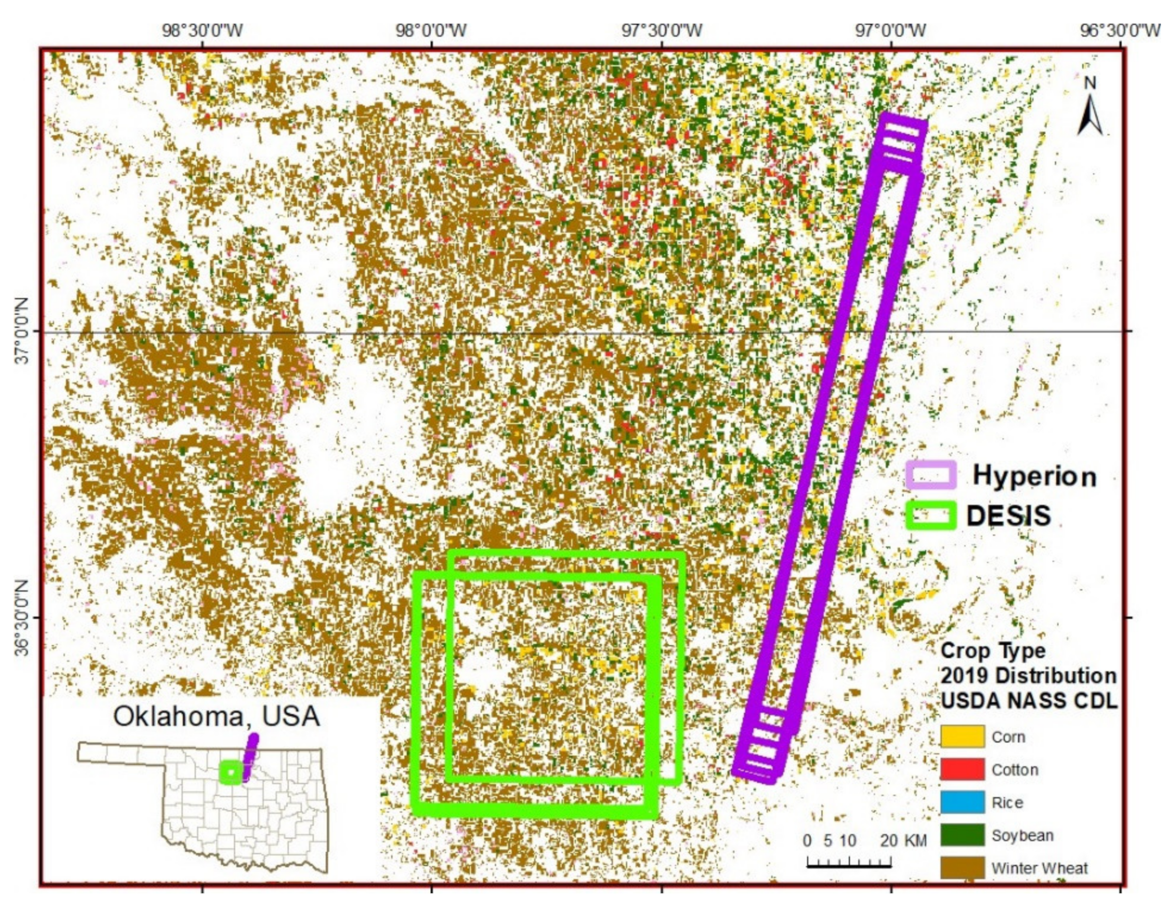
Figure 1. Hyperion and DESIS images. Hyperion and DESIS images used over Ponca City, Oklahoma, USA. CDL data source: [50].
Remotesensing 13 04704 g001
Figure 2. DESIS optimal bands. The twenty-nine optimal DESIS bands shown with example spectral profiles for corn and soybean.
Remotesensing 13 04704 g002
Figure 3. Average Hyperion 2010 (wet year) spectra by crop type for: (a) June (Julian Day 152), (b) August (Julian Day 222), and (c) September (Julian Day 245). N is number of spectra included in the average.
Remotesensing 13 04704 g003
Figure 4. Average Hyperion 2012 (normal year) spectra by crop type for: (a) July (Julian Day 200), (b) August (Julian Day 234), and (c) September (Julian Day 255). N is number of spectra included in the average.
Remotesensing 13 04704 g004
Figure 5. Average Hyperion 2013 (dry year) spectra by crop type for: (a) June (Julian Day 162), (b) July (Julian Day 191), (c) August (Julian Day 236), and (d) September (Julian Day 252). N is number of spectra included in the average.
Remotesensing 13 04704 g005
Figure 6. Average DESIS 2019 (wet year) spectra by crop type for: (a) June (Julian Day 172), (b) July (Julian Day 208), and (c) August (Julian Day 223). N is number of spectra included in the average.
Remotesensing 13 04704 g006
Figure 7. DESIS Corn Spectra for the year 2019 (wet year). DESIS corn spectra on Julian Days 172 (June), 208 (July), and 223 (August) in Oklahoma, USA.
Remotesensing 13 04704 g007
Figure 8. DESIS Soybean Spectra for the year 2019 (wet year). DESIS soybean spectra on Julian Days 172 (June), 208 (July), and 223 (August) in Oklahoma, USA.
Remotesensing 13 04704 g008
Table 1. Comparison of Hyperion and DESIS sensor characteristics.
HyperionDESIS
Sensor TypePolar-OrbitingOn MUSES platform of ISS
Years of Image Availability2001–20152019–present
Spectral Range356 to 2577 nm400 to 1000 nm
Number of Bands242235
Spectral Resolution10 nm2.55 nm
Spatial Resolution30 m30 m
Signal to Noise Ratio at 550 nm161195 with no binning
Radiometric Resolution12 bit13 bit
Table 2. Hyperion and DESIS images used. Timing of collected Hyperion and DESIS imagery and precipitation regime. All images contain samples of corn, soybean, and winter wheat spectra.
SensorImageAreaYearPrecipitation RegimeMonth
HyperionEO1H0280342010152110K7_PF2_01OK-12010WetJune
EO1H0280342010222110T6_SGS_01OK-12010WetAugust
EO1H0280342010245110P3_SGS_01OK-12010WetSeptember
EO1H0280342012200110K7_SGS_01OK-12012NormalJuly
EO1H0280342012234110K7_SGS_01OK-12012NormalAugust
EO1H0280342012255110P3_SGS_01OK-12012NormalSeptember
EO1H0280342013162110K7_SG1_01OK-12013DryJune
EO1H0280342013191110K7_SG1_01OK-12013DryJuly
EO1H0280342013236110K7_SG1_01OK-12013DryAugust
EO1H0280342013252110P3_SG1_01OK-12013DrySeptember
DESISDESIS-HSI-20190621T132231-001OK-22019WetJune
DESIS-HSI-20190727T230233-001OK-22019WetJuly
DESIS-HSI-20190811T170907-001OK-22019WetAugust
Table 3. Total samples. Hyperion and DESIS total samples. Hyperion samples were then split into training (37.5%), testing (37.5%), and validation (25%) subsets. Similarly, DESIS samples were split into training (33.3%), testing (33.3%), and validation (33.3%) subsets.
Number of Samples
SensorMonth, YearCornSoybeanWinter
Wheat
Other
Crop
Non-
Crop
Total
HyperionJune, 201026657528152346
August, 201017685228127292
September, 201022617428179364
July, 2012272711429142339
August, 201292411527139314
September, 2012262511425149339
June, 2013222314865176434
July, 2013212211143139336
August, 2013212412951179404
September, 2013192413949188419
DESISJune, 20193261112531454311266
July, 20194032543823525201911
August, 20193862373522924951762
Total Hyperion Samples 210363107137315703587
Total DESIS Samples 111560298778914464939
Total Samples 13259652058116230168526
Table 4. Most important DESIS bands. The 29 most important bands from DESIS data for vegetation classification, similar narrow bands selected by other researchers from multiple sensors, and applications for which the bands were used. LUE = Light-use efficiency, LAI = Leaf Area Index, LULC = Land use and land cover.
BandSimilar Narrow BandsApplicationReferences
(nm)
504502, 503, 504Disease, LAI[86,87,88,89]
522521, 528, 529LUE, stress, disease, LAI[3,86,87,88,89]
540531, 536, 541, 546LUE, stress, disease, crop growth stage classification[21,87,89,90,91]
556556, 557, 560Nitrogen, crop growth stage classification, pigments, weed detection[87,91,92,93]
574569, 570, 578Nitrogen, pigments, weed detection [3,21,90,92]
588589, 590Biomass/yield[12,87]
602599LULC classification [87]
614609, 613, 618LULC classification, LAI[86,87,88]
625627, 628, 630Biomass/yield, crop growth stage classification[12,87,91]
637632, 638, 640Biomass/yield, disease [12,86,87,89]
648648, 650Biomass/yield[21,87]
660657, 658, 665LULC classification, pigments, weed detection [86,87,92,93]
678677, 678, 680, 681Biomass/yield, disease, pigments, LAI, weed detection[3,88,89,92,93]
704703, 705, 709Stress, pigments, LAI[88,90,93]
718715, 720, 722Stress, pigments, crop growth stage classification[3,21,90,91]
740734, 738, 740, 742LULC classification, crop growth stage classification, LAI[87,88,91]
763754, 760, 763Biomass/yield, pigments [3,21,87,93]
778773, 774Biomass/yield, crop classification [12,87]
796793, 803Biomass/yield, crop classification [12,87]
824824Biomass/yield[12]
848844, 849, 852, 855Biomass/yield, pigments, disease, LAI [3,21,88,89,90]
866864, 869Crop classification[12,86]
885885Crop classification [12]
906909, 910Biomass/yield, pigments[21,86]
919915, 923Biomass/yield, pigments, crop growth stage classification[3,91]
934933, 938Biomass/yield, LAI [12,88]
945951, 953Biomass/yield, LAI[12,88]
960968, 970Moisture, biomass/yield, protein, growth stage classification, LAI [21,88,90,91]
979970, 973, 983Water absorption, LAI, crop classification, biomass/yield[12,86,88,91]
Table 5. Validation samples. Sample sizes in the validation subsets across all years for Hyperion classification analyses (2010, 2012, and 2013), and DESIS classification analyses for 2019.
Number of Samples
SensorImage(s) UsedCornSoybeanWinter Wheat
HyperionJune122256
July121356
August112974
September172781
June–July111152
June–August194087
June–September234296
July–August1422105
July–September2321106
August–September1951143
June–July–August161566
June–July–September161565
June–August–September2758127
July–August–September1931156
June–July–August–September211987
DESISJune1093784
July13485127
August12979117
June–July78245
June–August87229
July–August914911
Table 6. Hyperion Random Forest Accuracies. Classification accuracies for Random Forest separating three leading world crops (corn, soybean, and winter wheat) using 15 Hyperion narrowbands. Analysis was conducted across 3 years, for 4 months throughout each growing season when available; these accuracies are averages across those 3 years.
Image(s) UsedOverallProducer’s (User’s) Accuracies (%) *
Accuracy (%) *CornSoybeanWinter Wheat
June6842(53)44(32)76(72)
July6641(88)29(50)73(73)
August7132(33)72(72)75(78)
September7742(67)42(58)88(75)
June–July94100(100)64(100)96(93)
June–August9391(85)100(94)97(92)
June–September9591(95)91(92)100(100)
July–August94100(100)95(100)96(89)
July–September98100(100)88(100)100(97)
August–September9493(93)85(93)94(93)
June–July–August97100(100)100(100)100(92)
June–July–September100100(100)100(100)100(100)
June–August–September9691(100)94(98)100(98)
July–August–September99100(97)93(100)100(99)
June–July–August–September100100(100)100(100)100(100)
* These results are for the validation subset, which was not used for training and testing.
Table 7. Hyperion Support Vector Machine Accuracies. Classification accuracies for Support Vector Machine separating three leading world crops (corn, soybean, and winter wheat) using 15 Hyperion narrowbands. Analysis was conducted across 3 years, for 4 months throughout each growing season when available; these accuracies are averages across those 3 years.
Image(s) UsedOverallProducer’s (User’s) Accuracy (%)
Accuracy (%) *CornSoybeanWinter Wheat
June7750(48)60(53)88(82)
July7656(75)75(59)91(79)
August7623(23)87(66)75(84)
September7759(56)47(66)87(79)
June–July8982(90)100(100)92(86)
June–August9391(85)90(88)96(95)
June–September93100(82)98(91)96(95)
July–August93100(83)100(100)96(90)
July–September94100(93)96(100)99(95)
August–September91100(79)85(94)94(93)
June–July–August99100(100)100(100)100(97)
June–July–September100100(100)100(100)100(100)
June–August–September99100(97)100(98)100(100)
July–August–September99100(100)97(100)99(99)
June–July–August–September100100(100)100(100)100(100)
* These results are for the validation subset, which was not used for training and testing.
Table 8. Hyperion Naive Bayes Accuracies. Classification accuracies for Naive Bayes separating three leading world crops (corn, soybean, and winter wheat) using 15 Hyperion narrowbands. Analysis was conducted across 3 years, for 4 months throughout each growing season when available; these accuracies are averages across those 3 years.
Image(s) UsedOverallProducer’s (User’s) Accuracy (%)
Accuracy (%) *CornSoybeanWinter Wheat
June6617(100)92(50)76(65)
July6617(63)23(75)91(59)
August6717(25)70(70)77(75)
September6726(41)40(53)91(69)
June–July6891(67)82(56)81(66)
June–August7246(42)94(67)84(80)
June–September7775(42)78(76)86(83)
July–August7125(50)69(70)82(73)
July–September7981(68)54(79)94(78)
August–September7052(45)62(47)87(76)
June–July–August7588(82)93(64)86(80)
June–July–September86100(84)87(81)95(87)
June–August–September7970(48)90(78)93(84)
July–August–September7953(43)72(69)91(79)
June–July–August–September8290(79)89(68)91(86)
* These results are for the validation subset, which was not used for training and testing.
Table 9. Hyperion WekaXMeans Accuracies. Classification accuracies for WekaXMeans separating three leading world crops (corn, soybean, and winter wheat) using 15 Hyperion narrowbands. Analysis was conducted across 3 years, for 4 months throughout each growing season when available; these accuracies are averages across those 3 years.
Image(s) UsedOverallProducer’s (User’s) Accuracy (%)
Accuracy (%) *CornSoybeanWinter Wheat
June6050(23)73(46)80(72)
July3493(30)31(10)41(66)
August5433(12)88(58)57(77)
September6144(25)31(88)46(69)
June–July7082(45)73(57)87(69)
June–August7183(33)89(81)80(88)
June–September7745(25)86(69)91(86)
July–August6673(54)60(69)61(78)
July–September5986(47)47(46)68(83)
August–September6356(24)40(64)74(76)
June–July–August7581(87)73(65)86(70)
June–July–September7888(67)73(61)91(86)
June–August–September7674(41)71(80)91(93)
July–August–September7371(54)69(82)81(79)
June–July–August–September8881(94)89(89)93(89)
* These results are for the validation subset, which was not used for training and testing.
Table 10. DESIS Overall Accuracies. Overall classification accuracies for three leading world crops (corn, soybean, and winter wheat) from four classification algorithms (Random Forest, Support Vector Machine, Naive Bayes, and WekaXMeans) using 29 DESIS hyperspectral narrowbands. Analysis was conducted for June through August 2019.
Overall Accuracy (%) *
Image(s) UsedRandom ForestSupport Vector MachineNaive BayesWekaXMeans
June80705661
July68623442
August79655048
June–July78798063
June–August83857075
July–August67674457
* These results are for the validation subset, which was not used for training and testing.
Table 11. DESIS Producer’s and User’s Accuracies. Producer’s and user’s classification accuracies for three leading world crops (corn, soybean, and winter wheat) from four classification algorithms (Random Forest—RF, Support Vector Machine—SVM, Naive Bayes—NB, and WekaXMeans—WXM) using 29 DESIS hyperspectral narrowbands. Analysis was conducted for June through August, 2019. Soy = Soybean, WW = Winter Wheat.
Image(s) UsedProducer’s (User’s) Accuracies (%) *
CornRF
Soy
WWCornSVM
Soy
WWCornNB
Soy
WWCornWXM
Soy
WW
June91
(99)
81
(75)
69
(67)
98
(99)
70
(65)
49
(48)
89
(96)
76
(42)
62
(49)
90
(91)
38
(41)
63
(51)
July83
(74)
58
(80)
65
(64)
85
(68)
51
(74)
54
(64)
61
(38)
15
(21)
54
(37)
57
(43)
12
(38)
63
(48)
August85
(76)
80
(91)
61
(76)
81
(74)
73
(77)
53
(60)
74
(53)
61
(56)
47
(62)
55
(51)
54
(72)
56
(51)
June–July100
(87)
100
(63)
0
(0)
100
(98)
79
(59)
0
(0)
100
(96)
100
(55)
0 (NA)100
(78)
75
(78)
0
(0)
June–August84
(99)
77
(74)
11
(33)
89
(94)
82
(90)
56
(36)
80
(96)
86
(83)
56
(15)
92
(86)
82
(69)
33
(27)
July–August75
(78)
69
(92)
9
(33)
81
(80)
69
(92)
18
(13)
64
(73)
57
(45)
27
(6)
69
(65)
65
(51)
9
(10)
* These results are for the validation subset, which was not used for training and testing.
Publisher’s Note: MDPI stays neutral with regard to jurisdictional claims in published maps and institutional affiliations.