
Analysis of Landscape Connectivity among the Habitats of Asian Elephants in Keonjhar Forest Division, India

 ,
, 

Abstract
:
1. Introduction
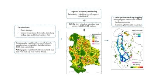
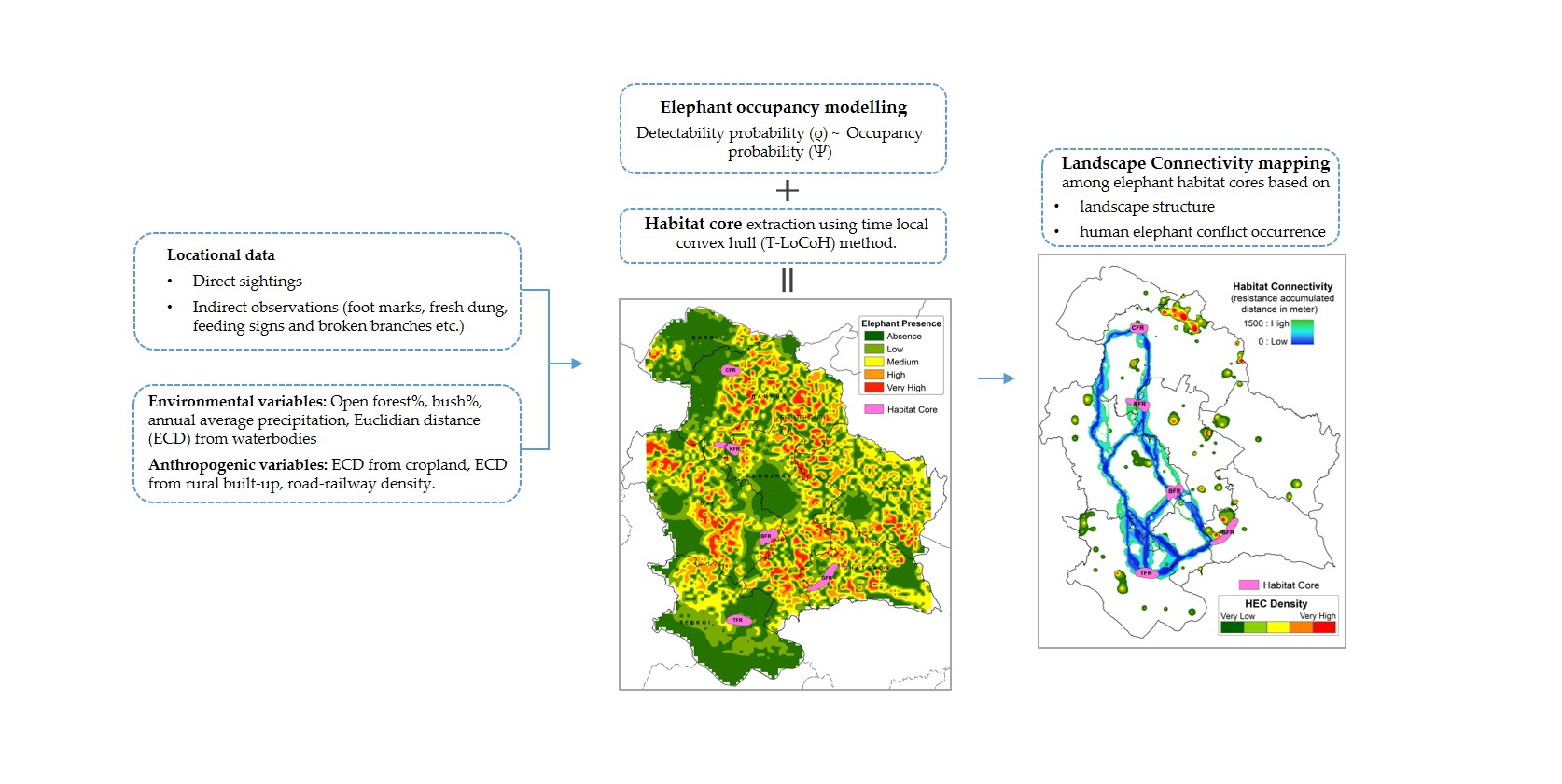
2. Materials and Methods
2.1. Study Area
2.2. Data Collection and Analysis
2.3. Occupancy Modelling and Habitat Core Estimation
2.4. Landscape Connectivity Analysis
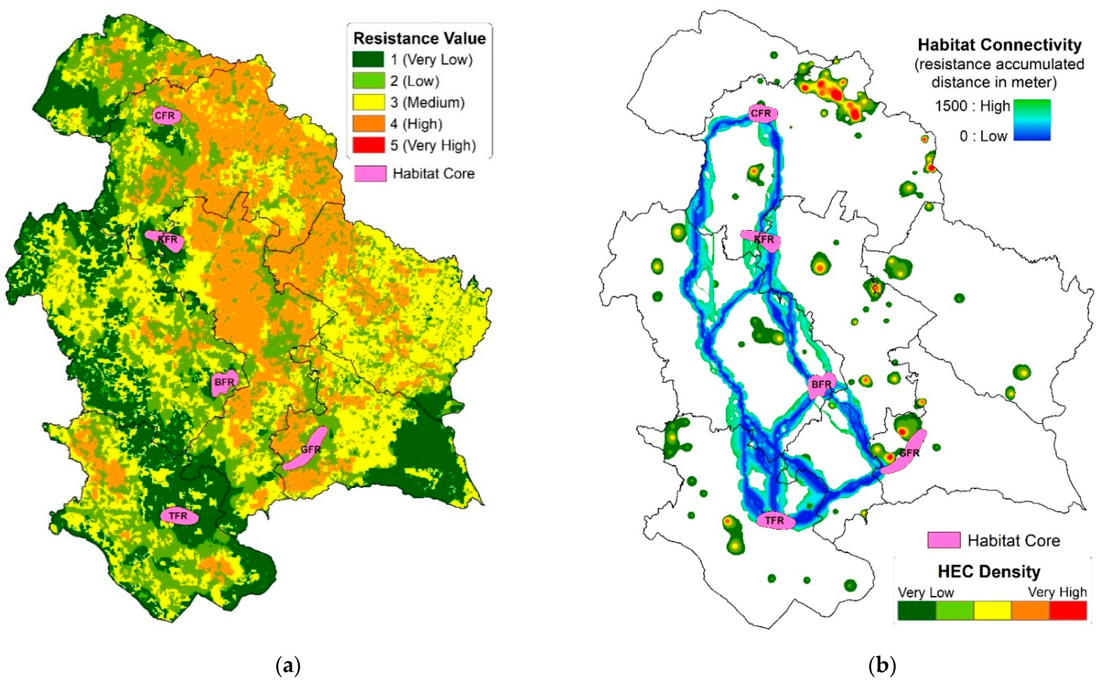
2.4.1. Resistance Surface
2.4.2. Mapping Elephant Movement Pathways
2.4.3. Assessing the Characteristics of Least-Resistant Paths
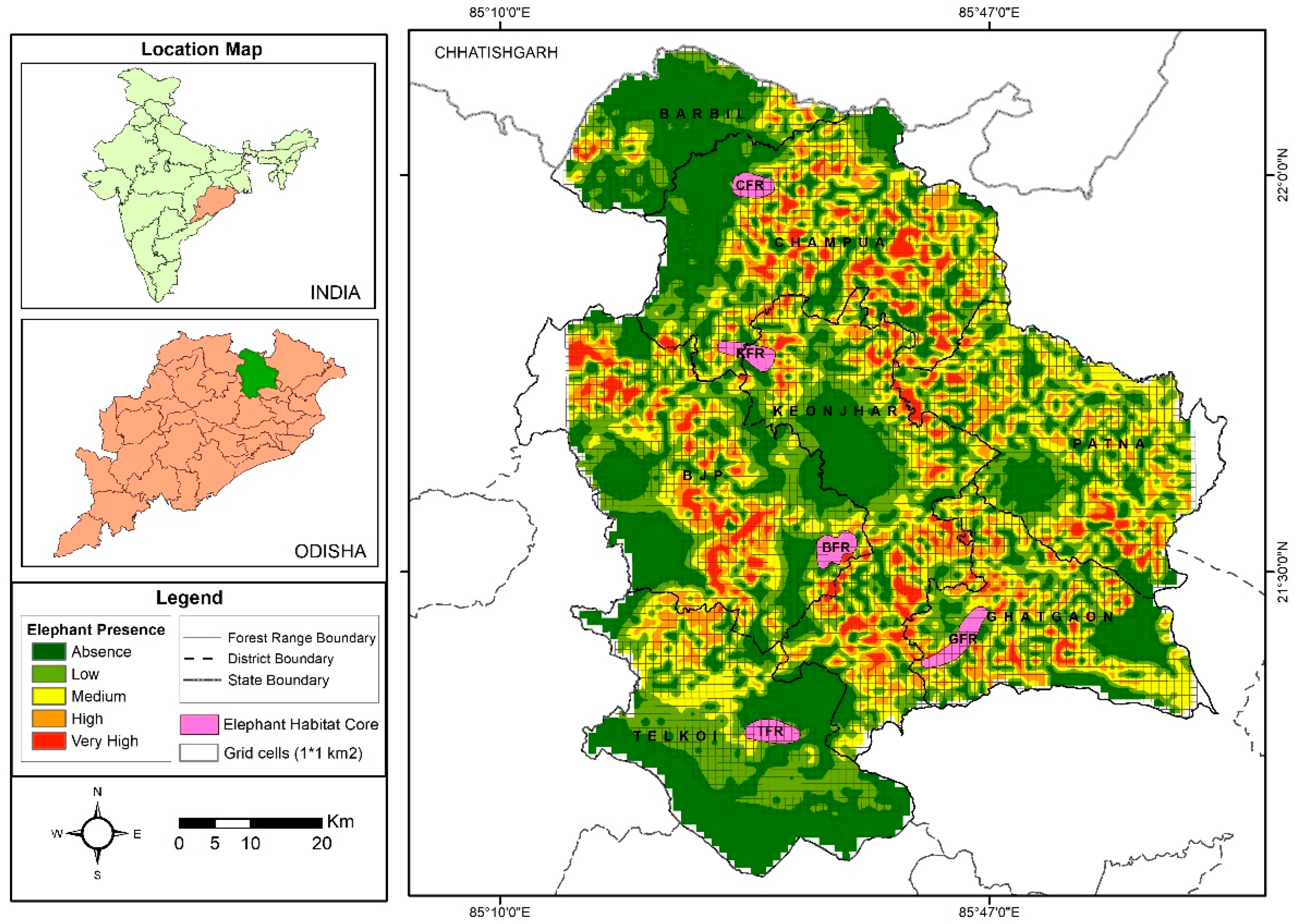
3. Results
3.1. Elephant Occupancy
3.2. Elephant Habitat Connectivity
4. Discussion
4.1. Variables Influencing Elephant Detection
4.2. Interpretation of the Characteristics of Estimated Connectivity
4.3. Implications and Recommendations
5. Conclusions
Supplementary Materials
Author Contributions
Funding
Acknowledgments
Conflicts of Interest
References
- Secretariat of the Convention on Biological Diversity. Global Biodiversity Outlook 3; Secretariat of the Convention on Biological Diversity: Montréal, QC, Canada, 2010. [Google Scholar]
- Shaffer, M.L. Minimum Population Sizes for Species Conservation. Bioscience 1981, 31, 131–134. [Google Scholar] [CrossRef]
- Fahrig, L. Effects of Habitat Fragmentation on Biodiversity. Annu. Rev. Ecol. Evol. Syst. 2003, 34, 487–515. [Google Scholar] [CrossRef] [Green Version]
- Pflüger, F.J.; Signer, J.; Balkenhol, N. Habitat loss causes non-linear genetic erosion in specialist species. Glob. Ecol. Conserv. 2019, 17, e00507. [Google Scholar] [CrossRef]
- Fischer, J.; Lindenmayer, D.B. Landscape modification and habitat fragmentation: A synthesis. Glob. Ecol. Biogeogr. 2007, 16, 265–280. [Google Scholar] [CrossRef]
- Januchowski-Hartley, S.; McIntyre, P.B.; Diebel, M.; Doran, P.J.; Infante, D.M.; Joseph, C.; Allan, J.D. Restoring aquatic ecosystem connectivity requires expanding inventories of both dams and road crossings. Front. Ecol. Environ. 2013, 11, 211–217. [Google Scholar] [CrossRef]
- Mimet, A.; Clauzel, C.; Foltête, J.-C. Locating wildlife crossings for multispecies connectivity across linear infrastructures. Landsc. Ecol. 2016, 31, 1955–1973. [Google Scholar] [CrossRef]
- International Union for the Conservation of Nature (IUCN). The IUCN Red List of Threatened Species Version 2018-1. 2018. Available online: https://www.iucnredlist.org/ (accessed on 9 September 2020).
- Crooks, K.R.; Burdett, C.L.; Theobald, D.M.; King, S.; Di Marco, M.; Rondinini, C.; Boitani, L. Quantification of habitat fragmentation reveals extinction risk in terrestrial mammals. Proc. Natl. Acad. Sci. USA 2017, 114, 7635–7640. [Google Scholar] [CrossRef] [Green Version]
- Campos-Arceiz, A.; Larrinaga, A.R.; Weerasinghe, U.R.; Takatsuki, S.; Pastorini, J.; Leimgruber, P.; Fernando, P.; Santamaría, L. Behavior rather than diet mediates seasonal differences in seed dispersal by Asian elephants. Ecology 2008, 89, 2684–2691. [Google Scholar] [CrossRef] [Green Version]
- Maisels, F.; Strindberg, S.; Blake, S.; Wittemyer, G.; Hart, J.; Williamson, E.; Aba’A, R.; Abitsi, G.; Ambahe, R.D.; Amsini, F.; et al. Devastating Decline of Forest Elephants in Central Africa. PLoS ONE 2013, 8, e59469. [Google Scholar] [CrossRef]
- Fritz, H. Long-term field studies of elephants: Understanding the ecology and conservation of a long-lived ecosystem engineer. J. Mammal. 2017, 98, 603–611. [Google Scholar] [CrossRef]
- Sekar, N.; Lee, C.; Sukumar, R. Functional nonredundancy of elephants in a disturbed tropical forest. Conserv. Biol. 2017, 31, 1152–1162. [Google Scholar] [CrossRef]
- Poulsen, J.R.; Rosin, C.; Meier, A.; Mills, E.; Nuñez, C.L.; Koerner, S.; Blanchard, E.; Callejas, J.; Moore, S.; Sowers, M. Ecological consequences of forest elephant declines for Afrotropical forests. Conserv. Biol. 2018, 32, 559–567. [Google Scholar] [CrossRef]
- Leimgruber, P.; Gagnon, J.B.; Wemmer, C.; Kelly, D.S.; Songer, M.A.; Selig, E.R. Fragmentation of Asia’s remaining wildlands: Implications for Asian elephant conservation. Anim. Conserv. 2003, 6, 347–359. [Google Scholar] [CrossRef] [Green Version]
- Sukumar, R. The Living Elephants: Evolutionary Ecology, Behaviour, and Conservation; Oxford University Press: Oxford, UK, 2003. [Google Scholar]
- IUCN/SSC Asian Elephant Specialist Group. Asian Elephant Range States Meeting: Final Report; Technical Report; The IUCN Species Survival Commission (SSC): Jakarta, Indonesia, 2017. [Google Scholar]
- Menon, V.; Tiwari, S.K.; Kyarong, S.; Ganguly, U.; Sukumar, R. Right of Passage: Elephant Corridors of India, 2nd ed.; Wildlife Trust of India: New Delhi, India, 2017. [Google Scholar]
- Kitratporn, N.; Takeuchi, W. Spatiotemporal Distribution of Human–Elephant Conflict in Eastern Thailand: A Model-Based Assessment Using News Reports and Remotely Sensed Data. Remote Sens. 2020, 12, 90. [Google Scholar] [CrossRef] [Green Version]
- Sukumar, R. A brief review of the status, distribution and biology of wild Asian elephants Elephas maximus. Int. Zoo Yearb. 2006, 40, 1–8. [Google Scholar] [CrossRef]
- Naha, D.; Sathyakumar, S.; Dash, S.; Chettri, A.; Rawat, G.S. Assessment and prediction of spatial patterns of human-elephant conflicts in changing land cover scenarios of a human-dominated landscape in North Bengal. PLoS ONE 2019, 14, e0210580. [Google Scholar] [CrossRef] [Green Version]
- Sengupta, A.; Binoy, V.V.; Radhakrishna, S. Human-Elephant Conflict in Kerala, India: A Rapid Appraisal Using Compensation Records. Hum. Ecol. 2020, 48, 101–109. [Google Scholar] [CrossRef]
- Moreira, F.; Rego, F.C.; Godinho-Ferreira, P. Temporal (1958–1995) pattern of change in a cultural landscape of northwestern Portugal: Implications for fire occurrence. Landsc. Ecol. 2001, 16, 557–567. [Google Scholar] [CrossRef]
- Desai, A.A. The home range of elephants and its implications for management of the Mudumalai wildlife sanctuary, Tamil Nadu. J. Bombay Nat. Hist. Soc. 1991, 88, 145–156. [Google Scholar]
- Madhusudan, M.D. Living Amidst Large Wildlife: Livestock and Crop Depredation by Large Mammals in the Interior Villages of Bhadra Tiger Reserve, South India. Environ. Manag. 2003, 31, 466–475. [Google Scholar] [CrossRef]
- Tripathy, B.R.; Liu, X.; Songer, M.; Kumar, L.; Kaliraj, S.; Das Chatterjee, N.; Wickramasinghe, W.M.S.; Mahanta, K.K. Descriptive Spatial Analysis of Human-Elephant Conflict (HEC) Distribution and Mapping HEC Hotspots in Keonjhar Forest Division, India. Front. Ecol. Evol. 2021, 9, 360. [Google Scholar] [CrossRef]
- MOEF. Gajah: Securing the Future for Elephants in India; Ministry of Environment and Forests (MOEF), Government of India: New Delhi, India, 2010.
- Hill, C.M.; Wallace, G.E. Crop protection and conflict mitigation: Reducing the costs of living alongside non-human primates. Biodivers. Conserv. 2012, 21, 2569–2587. [Google Scholar] [CrossRef]
- Pozo, R.A.; Coulson, T.; McCulloch, G.; Stronza, A.L.; Songhurst, A.C. Determining baselines for human-elephant conflict: A matter of time. PLoS ONE 2017, 12, e0178840. [Google Scholar] [CrossRef] [Green Version]
- Gaynor, K.M.; Branco, P.S.; Long, R.A.; Gonçalves, D.D.; Granli, P.K.; Poole, J.H. Effects of human settlement and roads on diel activity patterns of elephants (Loxodonta africana). Afr. J. Ecol. 2018, 56, 872–881. [Google Scholar] [CrossRef] [Green Version]
- Hoare, R.E.; Du Toit, J.T. Coexistence between People and Elephants in African Savannas. Conserv. Biol. 1999, 13, 633–639. [Google Scholar] [CrossRef]
- Loarie, S.R.; van Aarde, R.J.; Pimm, S.L. Fences and artificial water affect African savannah elephant movement patterns. Biol. Conserv. 2009, 142, 3086–3098. [Google Scholar] [CrossRef]
- Roever, C.; van Aarde, R.; Leggett, K. Functional connectivity within conservation networks: Delineating corridors for African elephants. Biol. Conserv. 2013, 157, 128–135. [Google Scholar] [CrossRef] [Green Version]
- Krishnan, V.; Kumar, M.A.; Raghunathan, G.; Vijayakrishnan, S. Distribution and Habitat Use by Asian Elephants (Elephas maximus) in a Coffee-Dominated Landscape of Southern India. Trop. Conserv. Sci. 2019, 12, 1940082918822599. [Google Scholar] [CrossRef]
- Lakshminarayanan, N.; Karanth, K.K.; Goswami, V.R.; Vaidyanathan, S.; Karanth, K.U. Determinants of dry season habitat use by Asian elephants in the Western Ghats of India. J. Zool. 2015, 298, 169–177. [Google Scholar] [CrossRef]
- Neupane, D.; Kwon, Y.; Risch, T.S.; Williams, A.C.; Johnson, R.L. Habitat use by Asian elephants: Context matters. Glob. Ecol. Conserv. 2019, 17, e00570. [Google Scholar] [CrossRef]
- Buij, R.; McShea, W.J.; Campbell, P.; Lee, M.E.; Dallmeier, F.; Guimondou, S.; Mackaga, L.; Guisseougou, N.; Mboumba, S.; Hines, J.E.; et al. Patch-occupancy models indicate human activity as major determinant of forest elephant Loxodonta cyclotis seasonal distribution in an industrial corridor in Gabon. Biol. Conserv. 2007, 135, 189–201. [Google Scholar] [CrossRef]
- Sitompul, A.F.; Griffin, C.R.; Rayl, N.D.; Fuller, T.K. Spatial and Temporal Habitat Use of an Asian Elephant in Sumatra. Animals 2013, 3, 670–679. [Google Scholar] [CrossRef] [PubMed]
- Sukumar, R. Ecology of the Asian elephant in southern India. II. Feeding habits and crop raiding patterns. J. Trop. Ecol. 1990, 6, 33–53. [Google Scholar] [CrossRef]
- Kumar, M.A.; Mudappa, D.; Raman, T.R.S. Asian Elephant Elephas Maximus Habitat Use and Ranging in Fragmented Rainforest and Plantations in the Anamalai Hills, India. Trop. Conserv. Sci. 2010, 3, 143–158. [Google Scholar] [CrossRef] [Green Version]
- Rood, E.; Ganie, A.A.; Nijman, V. Using presence-only modelling to predict Asian elephant habitat use in a tropical forest landscape: Implications for conservation. Divers. Distrib. 2010, 16, 975–984. [Google Scholar] [CrossRef]
- Kanagaraj, R.; Araujo, M.B.; Barman, R.; Davidar, P.; De, R.; Digal, D.K.; Gopi, G.V.; Johnsingh, A.J.T.; Kakati, K.; Kramer-Schadt, S.; et al. Predicting range shifts of Asian elephants under global change. Divers. Distrib. 2019, 25, 822–838. [Google Scholar] [CrossRef] [Green Version]
- Grand, J.B.; Williams, B.K.; Nichols, J.D.; Conroy, M.J. Analysis and Management of Animal Populations. J. Wildl. Manag. 2003, 67, 654. [Google Scholar] [CrossRef]
- Hedges, S. (Ed.) Monitoring Elephant Populations and Assessing Threats: A Manual for Researchers, Managers and Conservationists; Universities Press: Hyderabad, India, 2012. [Google Scholar]
- Yackulic, C.B.; Chandler, R.; Zipkin, E.F.; Royle, J.A.; Nichols, J.D.; Grant, E.H.C.; Veran, S. Presence-only modelling using MAXENT: When can we trust the inferences? Methods Ecol. Evol. 2013, 4, 236–243. [Google Scholar] [CrossRef]
- Karanth, K.U.; Gopalaswamy, A.M.; Kumar, N.S.; Vaidyanathan, S.; Nichols, J.D.; MacKenzie, D.I. Monitoring carnivore populations at the landscape scale: Occupancy modelling of tigers from sign surveys. J. Appl. Ecol. 2011, 48, 1048–1056. [Google Scholar] [CrossRef]
- MacKenzie, D.I.; Nichols, J.D.; Royle, J.A.; Pollock, K.H.; Hines, J.E.; Bailey, L.L. Occupancy Estimation and Modeling: Inferring Patterns and Dynamics of Species Occurrence; Elsevier: San Diego, CA, USA, 2006. [Google Scholar]
- MacKenzie, D.I.; Bailey, L.L. Assessing the fit of site-occupancy models. J. Agric. Biol. Environ. Stat. 2004, 9, 300–318. [Google Scholar] [CrossRef]
- Doerr, V.; Barrett, T.; Doerr, E. Connectivity, dispersal behaviour and conservation under climate change: A response to Hodgson et al. J. Appl. Ecol. 2010, 48, 143–147. [Google Scholar] [CrossRef]
- Holderegger, R.; Wagner, H.H. Landscape Genetics. Bioscience 2008, 58, 199–207. [Google Scholar] [CrossRef] [Green Version]
- Baguette, M.; van Dyck, H. Landscape connectivity and animal behavior: Functional grain as a key determinant for dispersal. Landsc. Ecol. 2007, 22, 1117–1129. [Google Scholar] [CrossRef]
- Spear, S.F.; Balkenhol, N.; Fortin, M.-J.; McRae, B.H.; Scribner, K.T. Use of resistance surfaces for landscape genetic studies: Considerations for parameterization and analysis. Mol. Ecol. 2010, 19, 3576–3591. [Google Scholar] [CrossRef]
- Cushman, S.A.; Lewis, J.S.; Landguth, E.L. Why Did the Bear Cross the Road? Comparing the Performance of Multiple Resistance Surfaces and Connectivity Modeling Methods. Diversity 2014, 6, 844–854. [Google Scholar] [CrossRef] [Green Version]
- Cushman, S.A.; Chase, M.; Griffin, C. Mapping Landscape Resistance to Identify Corridors and Barriers for Elephant Movement in Southern Africa. In Spatial Complexity, Informatics, and Wildlife Conservation; Springer: Singapore, 2010; pp. 349–367. [Google Scholar]
- Elliot, N.B.; Cushman, S.A.; Macdonald, D.W.; Loveridge, A.J. The devil is in the dispersers: Predictions of landscape connectivity change with demography. J. Appl. Ecol. 2014, 51, 1169–1178. [Google Scholar] [CrossRef]
- Moilanen, A.; Nieminen, M. Simple connectivity measures in spatial ecology. Ecology 2002, 83, 1131–1145. [Google Scholar] [CrossRef]
- Cushman, S.A.; Landguth, E.L.; Flather, C.H. Evaluating population connectivity for species of conservation concern in the American Great Plains. Biodivers. Conserv. 2013, 22, 2583–2605. [Google Scholar] [CrossRef] [Green Version]
- Thatte, P.; Joshi, A.; Vaidyanathan, S.; Landguth, E.; Ramakrishnan, U. Maintaining tiger connectivity and minimizing extinction into the next century: Insights from landscape genetics and spatially-explicit simulations. Biol. Conserv. 2018, 218, 181–191. [Google Scholar] [CrossRef]
- Buchholtz, E.K.; Stronza, A.; Songhurst, A.; McCulloch, G.; Fitzgerald, L.A. Using landscape connectivity to predict human-wildlife conflict. Biol. Conserv. 2020, 248, 108677. [Google Scholar] [CrossRef]
- Liu, C.; Newell, G.; White, M.; Bennett, A.F. Identifying wildlife corridors for the restoration of regional habitat connectivity: A multispecies approach and comparison of resistance surfaces. PLoS ONE 2018, 13, e0206071. [Google Scholar] [CrossRef]
- Osborn, F.V.; Parker, G.E. Linking two elephant refuges with a corridor in the communal lands of Zimbabwe. Afr. J. Ecol. 2003, 41, 68–74. [Google Scholar] [CrossRef]
- Menke, K. Locating Potential Cougar (Puma concolor) Corridors in New Mexico Using a Least-Cost Path Corridor GIS Analysis; NM Wildl. Final Proj. Report; Bird’s Eye View: Albuquerque, NM, USA, 2008. [Google Scholar]
- Koirala, R.K.; Raubenheimer, D.; Aryal, A.; Pathak, M.L.; Ji, W. Feeding preferences of the Asian elephant (Elephas maximus) in Nepal. BMC Ecol. 2016, 16, 54. [Google Scholar] [CrossRef] [Green Version]
- Li, W.; Liu, P.; Guo, X.; Wang, L.; Wang, Q.; Yu, Y.; Dai, Y.; Li, L.; Zhang, L. Human-elephant conflict in Xishuangbanna Prefecture, China: Distribution, diffusion, and mitigation. Glob. Ecol. Conserv. 2018, 16, e00462. [Google Scholar] [CrossRef]
- McRae, B.H. Centrality Mapper Connectivity Analysis Software; The Nature Conservancy: Seattle, WA, USA, 2012. [Google Scholar]
- McRae, B.H.; Dickson, B.G.; Keitt, T.H.; Shah, V.B. Using circuit theory to model connectivity in ecology, evolution, and conservation. Ecology 2008, 89, 2712–2724. [Google Scholar] [CrossRef]
- Anantharaman, R.; Hall, K.; Shah, V.B.; Edelman, A. Circuitscape in Julia: High Performance Connectivity Modelling to Support Conservation Decisions. JuliaCon Proc. 2020, 1, 58. [Google Scholar]
- Suksavate, W.; Duengkae, P.; Chaiyes, A. Quantifying landscape connectivity for wild Asian elephant populations among fragmented habitats in Thailand. Glob. Ecol. Conserv. 2019, 19, e00685. [Google Scholar] [CrossRef]
- Cushman, S.A.; Elliot, N.B.; Bauer, D.; Kesch, K.; Bahaa-El-Din, L.; Bothwell, H.; Flyman, M.; Mtare, G.; Macdonald, D.W.; Loveridge, A.J. Prioritizing core areas, corridors and conflict hotspots for lion conservation in southern Africa. PLoS ONE 2018, 13, e0196213. [Google Scholar] [CrossRef]
- Ghoddousi, A.; Bleyhl, B.; Sichau, C.; Ashayeri, D.; Moghadas, P.; Sepahvand, P.; Hamidi, A.K.; Soofi, M.; Kuemmerle, T. Mapping connectivity and conflict risk to identify safe corridors for the Persian leopard. Landsc. Ecol. 2020, 35, 1809–1825. [Google Scholar] [CrossRef]
- Puyravaud, J.-P.; Cushman, S.A.; Davidar, P.; Madappa, D. Predicting landscape connectivity for the Asian elephant in its largest remaining subpopulation. Anim. Conserv. 2017, 20, 225–234. [Google Scholar] [CrossRef]
- Huang, C.; Li, X.; Khanal, L.; Jiang, X. Habitat suitability and connectivity inform a co-management policy of protected area network for Asian elephants in China. PeerJ 2019, 7, e6791. [Google Scholar] [CrossRef] [PubMed]
- Osipova, L.; Okello, M.M.; Njumbi, S.J.; Ngene, S.; Western, D.; Hayward, M.W.; Balkenhol, N. Using step-selection functions to model landscape connectivity for African elephants: Accounting for variability across individuals and seasons. Anim. Conserv. 2019, 22, 35–48. [Google Scholar] [CrossRef]
- Carroll, C.; McRAE, B.H.; Brookes, A. Use of Linkage Mapping and Centrality Analysis Across Habitat Gradients to Conserve Connectivity of Gray Wolf Populations in Western North America. Conserv. Biol. 2012, 26, 78–87. [Google Scholar] [CrossRef] [PubMed]
- Castilho, C.S.; Hackbart, V.C.S.; Pivello, V.R.; Dos Santos, R.F. Evaluating Landscape Connectivity for Puma concolor and Panthera onca Among Atlantic Forest Protected Areas. Environ. Manag. 2015, 55, 1377–1389. [Google Scholar] [CrossRef]
- Vasudev, D.; Goswami, V.R.; Srinivas, N.; Syiem, B.L.N.; Sarma, A. Identifying important connectivity areas for the wide-ranging Asian elephant across conservation landscapes of Northeast India. Divers. Distrib. 2021. [Google Scholar] [CrossRef]
- Vasudev, D.; Fletcher, R.J.; Goswami, V.; Krishnadas, M. From dispersal constraints to landscape connectivity: Lessons from species distribution modeling. Ecography 2015, 38, 967–978. [Google Scholar] [CrossRef]
- Goswami, V.R.; Vasudev, D. Triage of Conservation Needs: The Juxtaposition of Conflict Mitigation and Connectivity Considerations in Heterogeneous, Human-Dominated Landscapes. Front. Ecol. Evol. 2017, 4, 144. [Google Scholar] [CrossRef] [Green Version]
- Vihar, S.; Baripada, S.; Palei, N.; Palei, H.; Sahu, H. Human-Elephant Conflict in Keonjhar, Odisha: Implications for Conservation; North Orissa University Press: Odisha, India, 2012. [Google Scholar]
- Wildlife Odisha. Wildlife Organisation, Forest & Environment Department, Govt. of Odisha, Bhubaneswar. 2020. Available online: http://www.wildlife.odisha.gov.in/assets/javaupload/publication/publication_1_Wil_2021-09-29T12:33:33.013412.pdf (accessed on 10 May 2021).
- Pettorelli, N.; Vik, J.O.; Mysterud, A.; Gaillard, J.-M.; Tucker, C.J.; Stenseth, N.C. Using the satellite-derived NDVI to assess ecological responses to environmental change. Trends Ecol. Evol. 2005, 20, 503–510. [Google Scholar] [CrossRef]
- Bohrer, G.; Beck, P.S.; Ngene, S.M.; Skidmore, A.K.; Douglas-Hamilton, I. Elephant movement closely tracks precipitation-driven vegetation dynamics in a Kenyan forest-savanna landscape. Mov. Ecol. 2014, 2, 2. [Google Scholar] [CrossRef] [Green Version]
- Liu, H.Q.; Huete, A. A feedback based modification of the NDVI to minimize canopy background and atmospheric noise. IEEE Trans. Geosci. Remote Sens. 1995, 33, 457–465. [Google Scholar] [CrossRef]
- Santiapillai, C.; Wijeyamohan, S. Conservation and the History of Human–Elephant Relations in Sri Lanka. In Conflict, Negotiation, and Coexistence: Rethinking Human–Elephant Relations in South Asia; Oxford University Press: Oxford, UK, 2016; pp. 229–241. [Google Scholar]
- Saatchi, S.; Buermann, W.; ter Steege, H.; Mori, S.; Smith, T.B. Modeling distribution of Amazonian tree species and diversity using remote sensing measurements. Remote Sens. Environ. 2008, 112, 2000–2017. [Google Scholar] [CrossRef]
- Rowe, M.F.; Bakken, G.S.; Ratliff, J.J.; Langman, V.A. Heat storage in Asian elephants during submaximal exercise: Behavioral regulation of thermoregulatory constraints on activity in endothermic gigantotherms. J. Exp. Biol. 2013, 216, 1774–1785. [Google Scholar] [CrossRef] [Green Version]
- Shannon, G.; Matthews, W.S.; Page, B.R.; Parker, G.E.; Smith, R.J. The affects of artificial water availability on large herbivore ranging patterns in savanna habitats: A new approach based on modelling elephant path distributions. Divers. Distrib. 2009, 15, 776–783. [Google Scholar] [CrossRef]
- Bhagat, V.K.; Yadav, D.K.; Jhariya, M.K. Human-Elephant Conflict and Its Consequences: A Preliminary Appraisal and Way Forward. Environ. Pharmacol. Life Sci. 2017, 6, 85–94. [Google Scholar]
- Wilson, S.; Davies, T.E.; Hazarika, N.; Zimmermann, A. Understanding spatial and temporal patterns of human–elephant conflict in Assam, India. Oryx 2015, 49, 140–149. [Google Scholar] [CrossRef] [Green Version]
- Gross, E.M.; Lahkar, B.P.; Subedi, N.; Nyirenda, V.R.; Lichtenfeld, L.L.; Jakoby, O. Seasonality, crop type and crop phenology influence crop damage by wildlife herbivores in Africa and Asia. Biodivers. Conserv. 2018, 27, 2029–2050. [Google Scholar] [CrossRef]
- Chartier, L.; Zimmermann, A.; Ladle, R.J. Habitat loss and human–elephant conflict in Assam, India: Does a critical threshold exist? Oryx 2011, 45, 528–533. [Google Scholar] [CrossRef] [Green Version]
- Naha, D.; Dash, S.K.; Chettri, A.; Roy, A.; Sathyakumar, S. Elephants in the neighborhood: Patterns of crop-raiding by Asian elephants within a fragmented landscape of Eastern India. PeerJ 2020, 8, e9399. [Google Scholar] [CrossRef]
- Santiapillai, C.; Chambers, M.; Ishwaran, N. Aspects of the ecology of the Asian elephant Elephas maximus L. in the Ruhuna National Park, Sri Lanka. Biol. Conserv. 1984, 29, 47–61. [Google Scholar] [CrossRef]
- Anuradha, J.M.P.N.; Fujimura, M.; Inaoka, T.; Sakai, N. The Role of Agricultural Land Use Pattern Dynamics on Elephant Habitat Depletion and Human-Elephant Conflict in Sri Lanka. Sustainability 2019, 11, 2818. [Google Scholar] [CrossRef] [Green Version]
- Jha, N.; Sarma, K.; Bhattacharya, P. Assessment of Elephant (Elephas Maximus) Mortality along Palakkad-Coimbatore Railway Stretch of Kerala and Tamil Nadu Using Geospatial Technology. J. Biodivers. Manag. For. 2014, 31, 2. [Google Scholar]
- Palei, N.C.; Palei, H.S.; Rath, B.P.; Kar, C.S. Mortality of the Endangered Asian elephant Elephas maximus by electrocution in Odisha, India. Oryx 2014, 48, 602–604. [Google Scholar] [CrossRef] [Green Version]
- Dasgupta, S.; Ghosh, A.K. Elephant–Railway Conflict in a Biodiversity Hotspot: Determinants and Perceptions of the Conflict in Northern West Bengal, India. Hum. Dimens. Wildl. 2014, 20, 81–94. [Google Scholar] [CrossRef]
- Zeller, K.A.; Nijhawan, S.; Salom-Pérez, R.; Potosme, S.H.; Hines, J.E. Integrating occupancy modeling and interview data for corridor identification: A case study for jaguars in Nicaragua. Biol. Conserv. 2011, 144, 892–901. [Google Scholar] [CrossRef]
- MacKenzie, D.I.; Nichols, J.D.; Lachman, G.B.; Droege, S.; Andrew Royle, J.; Langtimm, C.A. Estimating site occupancy rates when detection probabilities are less than one. Ecology 2002, 83, 2248–2255. [Google Scholar] [CrossRef]
- MacKenzie, D.I.; Royle, J.A.; Brown, J.A.; Nichols, J.D.; Thompson, W.L. Occupancy estimation and modeling for rare and elusive populations. In Sampling Rare or Elusive Species: Concepts, Designs, and Techniques for Estimating Population Parameters; Island Press: Washington, DC, USA, 2004; pp. 149–171. [Google Scholar]
- Milchev, B. Breeding biology of the Long-legged Buzzard Buteo rufinus in SE Bulgaria, nesting also in quarries. Avocetta 2009, 33, 25–32. [Google Scholar] [CrossRef]
- Zhang, J.; Jiang, F.; Li, G.; Qin, W.; Li, S.; Gao, H.; Cai, Z.; Lin, G.; Zhang, T. Maxent modeling for predicting the spatial distribution of three raptors in the Sanjiangyuan National Park, China. Ecol. Evol. 2019, 9, 6643–6654. [Google Scholar] [CrossRef] [Green Version]
- Jathanna, D.; Karanth, K.U.; Kumar, N.S.; Karanth, K.K.; Goswami, V.R. Patterns and Determinants of Habitat Occupancy by the Asian Elephant in the Western Ghats of Karnataka, India. PLoS ONE 2015, 10, e0133233. [Google Scholar] [CrossRef] [Green Version]
- Getz, W.M.; Wilmers, C.C. A local nearest-neighbor convex-hull construction of home ranges and utilization distributions. Ecography 2004, 27, 489–505. [Google Scholar] [CrossRef] [Green Version]
- Lyons, A.J.; Turner, W.C.; Getz, W.M. Home range plus: A space-time characterization of movement over real landscapes. Mov. Ecol. 2013, 1, 2. [Google Scholar] [CrossRef] [Green Version]
- Wilson, R.R.; Hooten, M.B.; Strobel, B.N.; Shivik, J.A. Accounting for Individuals, Uncertainty, and Multiscale Clustering in Core Area Estimation. J. Wildl. Manag. 2010, 74, 1343–1352. [Google Scholar] [CrossRef] [Green Version]
- Elith, J.; Leathwick, J.R. Species Distribution Models: Ecological Explanation and Prediction Across Space and Time. Annu. Rev. Ecol. Evol. Syst. 2009, 40, 677–697. [Google Scholar] [CrossRef]
- Compton, B.W.; McGARIGAL, K.; Cushman, S.A.; Gamble, L.R. A Resistant-Kernel Model of Connectivity for Amphibians that Breed in Vernal Pools. Conserv. Biol. 2007, 21, 788–799. [Google Scholar] [CrossRef] [PubMed]
- McClure, M.L.; Hansen, A.J.; Inman, R.M. Connecting models to movements: Testing connectivity model predictions against empirical migration and dispersal data. Landsc. Ecol. 2016, 31, 1419–1432. [Google Scholar] [CrossRef]
- Kent, M. Biogeography and landscape ecology: The way forward—Gradients and graph theory. Prog. Phys. Geogr. Earth Environ. 2009, 33, 424–436. [Google Scholar] [CrossRef]
- Zetterberg, A.; Mörtberg, U.; Balfors, B. Making graph theory operational for landscape ecological assessments, planning, and design. Landsc. Urban Plan. 2010, 95, 181–191. [Google Scholar] [CrossRef]
- Urban, D.; Keitt, T. Landscape connectivity: A graph-theoretic perspective. Ecology 2001, 82, 1205–1218. [Google Scholar] [CrossRef]
- McRae, B.H.; Kavanagh, D.M. Linkage Mapper Connectivity Analysis Software; Nature Conservancy: Seattle, WA, USA, 2011. [Google Scholar]
- Evans, L.J.; Asner, G.P.; Goossens, B. Protected area management priorities crucial for the future of Bornean elephants. Biol. Conserv. 2018, 221, 365–373. [Google Scholar] [CrossRef]
- Meijer, J.R.; Huijbregts, M.A.J.; Schotten, K.C.G.J.; Schipper, A.M. Global patterns of current and future road infrastructure. Environ. Res. Lett. 2018, 13, 64006. [Google Scholar] [CrossRef] [Green Version]
- Goswami, V.R.; Sridhara, S.; Medhi, K.; Williams, A.C.; Chellam, R.; Nichols, J.D.; Oli, M.K. Community-managed forests and wildlife-friendly agriculture play a subsidiary but not substitutive role to protected areas for the endangered Asian elephant. Biol. Conserv. 2014, 177, 74–81. [Google Scholar] [CrossRef]
- Chen, L.; Ouyang, Z.-Y.; Wang, X.-K.; Miao, H.; Duan, X.-N. Applications of contingent valuation method in evaluation of non-market values. Acta Ecol. Sin. 2006, 26, 610–619. [Google Scholar]
- De Boer, W.F.; Ntumi, C.P.; Correia, A.U.; Mafuca, J.M. Diet and distribution of elephant in the Maputo Elephant Reserve, Mozambique. Afr. J. Ecol. 2000, 38, 188–201. [Google Scholar] [CrossRef]
- Little, S.J.; Harcourt, R.; Clevenger, A.P. Do wildlife passages act as prey-traps? Biol. Conserv. 2002, 107, 135–145. [Google Scholar] [CrossRef]
- Kramer-Schadt, S.; Kaiser, T.; Frank, K.; Wiegand, T. Analyzing the effect of stepping stones on target patch colonisation in structured landscapes for Eurasian lynx. Landsc. Ecol. 2011, 26, 501–513. [Google Scholar] [CrossRef]
- Northrup, J.M.; Stenhouse, G.B.; Boyce, M.S. Agricultural lands as ecological traps for grizzly bears. Anim. Conserv. 2012, 15, 369–377. [Google Scholar] [CrossRef]
- Frankham, R. Genetics and conservation biology. Comptes Rendus Biol. 2003, 326, 22–29. [Google Scholar] [CrossRef]


| Variable | Category | Resistance Score | Weightage | |
|---|---|---|---|---|
| LULC | Bush/Scrub | 5 | 2 | |
| Open Forest | 1 | |||
| Dense Forest | 20 | |||
| Rural built-up | 80 | |||
| Urban development | 100 | |||
| Agriculture | 75 | |||
| Barren | 15 | |||
| Water bodies | River | 20 | 3 | |
| Canal/Drain | 40 | |||
| Reservoir/Tank | 5 | |||
| Lake/Pond | 5 | |||
| Mining | Active Mining and Quarry | 90 | 2 | |
| Industrial Areas | 100 | |||
| Waste and abandoned area | 80 | |||
| Railway | Absent | 1 | 1 | |
| Present | 100 | |||
| Road | Absent | 1 | 2 | |
| Present (Major) | 100 | |||
| Present (Minor) | 60 | |||
| Slope | High | 85 | 3 | |
| Medium | 50 | |||
| Low | 1 | |||
| Population Density | Absent | 1 | 1 | |
| Low | 30 | |||
| Medium | 60 | |||
| High | 100 | |||
| HEC Density | High | 90 | 3 | |
| Medium | 60 | |||
| Low | 20 | |||
| Scheme | Model | AIC | ΔAIC |
|---|---|---|---|
| Covariates selection | |||
| 1 | ρ (Open forest %) ~ Ψ (1) | 882.31 | 0 |
| 2 | ρ (Precipitation) ~ Ψ (1) | 882.66 | 0.35 |
| 3 | ρ (ECD_cropland) ~ Ψ (1) | 883.04 | 0.73 |
| 4 | ρ (ECD_rural) ~ Ψ (1) | 883.79 | 1.48 |
| 5 | ρ (Road–railway density) ~ Ψ (1) | 883.86 | 1.55 |
| 6 | ρ (Bush %) ~ Ψ (1) | 884.02 | 1.71 |
| 7 | ρ (ECD_waterbodies) ~ Ψ (1) | 884.31 | 2.00 |
| 8 | ρ (EVI) ~ Ψ (1) | 884.62 | 2.03 |
| Detection model | |||
| 1 | ρ (Open forest % + Precipitation + ECD_cropland + ECD_rural) ~ Ψ (1) | 1123.86 | 0 |
| 2 | ρ (Open forest % + Precipitation + ECD_cropland + ECD_rural + Road–railway density + Bush %) ~ Ψ (1) | 894.04 | 0.18 |
| 3 | ρ (Open forest % + Precipitation + ECD_cropland + Road–railway density) ~ Ψ (1) | 894.57 | 0.71 |
| 4 | ρ (Open forest % + ECD_cropland + Road–railway density + ECD_rural) ~ Ψ (1) | 895.24 | 1.38 |
| 5 | ρ (Open forest % + ECD_cropland + ECD_rural + Bush % + ECD_waterbodies) ~ Ψ (1) | 895.95 | 2.09 |
| Occupancy model | |||
| 1 | ρ (Open forest % + Precipitation + ECD_cropland + ECD_rural) ~ Ψ (Open forest % + Precipitation + ECD_cropland + ECD_rural + Road–railway density) | 894.63 | 0 |
| 2 | ρ (Open forest % + Precipitation + ECD_cropland + ECD_rural) ~ Ψ (ECD_cropland + Precipitation + Road–railway density + Bush %) | 895.12 | 0.49 |
| 3 | ρ (Open forest % + Precipitation + ECD_cropland + ECD_rural) ~ Ψ (Open forest % + Precipitation + ECD_cropland + ECD_rural + Road–railway density + Bush %) | 895.96 | 1.33 |
| 4 | ρ (Open forest % + Precipitation + ECD_cropland + ECD_rural) ~ Ψ (Open forest % + ECD_rural + Road–railway density + Bush % + ECD_waterbodies) | 896.54 | 1.91 |
| 5 | ρ (Open forest % + Precipitation + ECD_cropland + ECD_rural) ~ Ψ (Open forest % + ECD_cropland + ECD_rural + ECD_road–railway + ECD_waterbodies) | 896.87 | 2.24 |
| Model | Estimate | SE |
|---|---|---|
| Detectability | ||
| Intercept | 2.21 | 0.11 |
| Open forest % | 1.68 | 0.51 |
| Precipitation | 0.20 | 0.35 |
| ECD_cropland | −0.74 | 0.09 |
| ECD_rural | 0.13 | 0.89 |
| Occupancy | ||
| Intercept | 0.96 | 0.04 |
| Open forest % | 2.17 | 0.16 |
| Precipitation | 0.32 | 0.22 |
| ECD_cropland | −1.17 | 0.07 |
| Bush % | −0.09 | 1.08 |
| ECD_rural | 0.03 | 0.61 |
| Road–railway density | −2.32 | 0.13 |
| (A) | |||||||
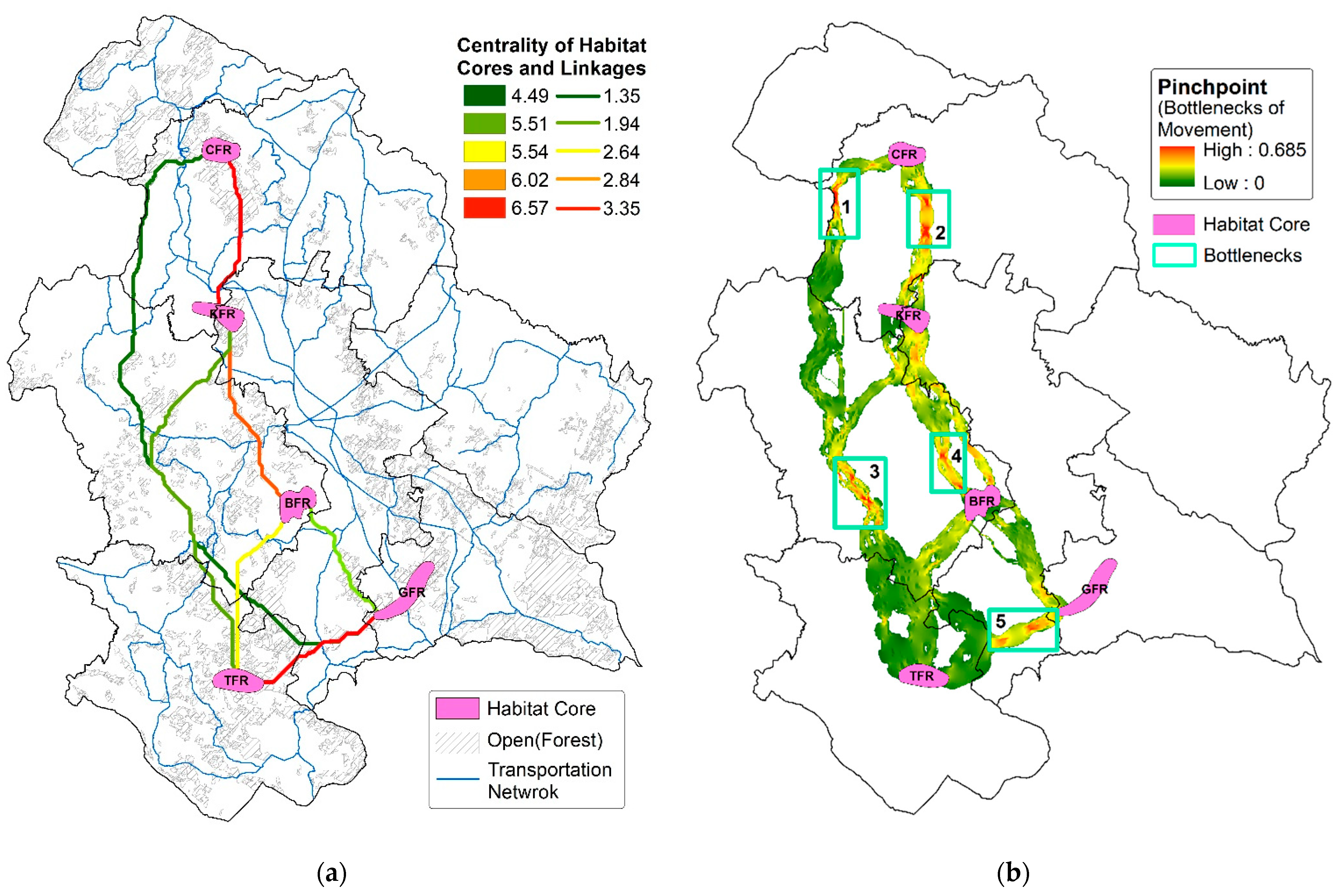
| Habitat Core | Area (m2) | Habitat Core Centrality | |||||
| CFR | 1,55,57,714.91 | 4.49561 | |||||
| BFR | 1,85,89,494.01 | 5.51905 | |||||
| TFR | 1,90,63,388.80 | 5.54219 | |||||
| GFR | 2,35,76,210.22 | 6.02567 | |||||
| KFR | 1,78,06,542.70 | 6.57972 | |||||
| (B) | |||||||
| From_Core | To_Core | Ed (meter) | Ra (meter) | Lr (meter) | Ra:Ed | Ra:Lr | Movement Flow Centrality |
| GFR | TFR | 18,360 | 24,576 | 19,769 | 1.33856 | 1.24372 | 2.8322 |
| TFR | BFR | 21,943 | 29,728 | 24,519 | 1.35478 | 1.21261 | 2.4845 |
| TFR | KFR | 48,458 | 71,124 | 59,573 | 1.46772 | 1.1939 | 1.7817 |
| KFR | CFR | 20,295 | 35,989 | 22,765 | 1.77325 | 1.58085 | 3.3494 |
| GFR | CFR | 64,157 | 11,831 | 10,314 | 1.84427 | 1.14769 | 1.6431 |
| BFR | KFR | 24,118 | 44,516 | 26,566 | 1.84575 | 1.65803 | 2.6478 |
| GFR | KFR | 42,811 | 89,507 | 73,149 | 2.09076 | 1.22627 | 1.3545 |
| GFR | BFR | 17,150 | 41,882 | 19,772 | 2.44219 | 2.11857 | 1.9408 |
Publisher’s Note: MDPI stays neutral with regard to jurisdictional claims in published maps and institutional affiliations. |
© 2021 by the authors. Licensee MDPI, Basel, Switzerland. This article is an open access article distributed under the terms and conditions of the Creative Commons Attribution (CC BY) license (https://creativecommons.org/licenses/by/4.0/).
Share and Cite
Tripathy, B.R.; Liu, X.; Songer, M.; Zahoor, B.; Wickramasinghe, W.M.S.; Mahanta, K.K. Analysis of Landscape Connectivity among the Habitats of Asian Elephants in Keonjhar Forest Division, India. Remote Sens. 2021, 13, 4661. https://doi.org/10.3390/rs13224661
Tripathy BR, Liu X, Songer M, Zahoor B, Wickramasinghe WMS, Mahanta KK. Analysis of Landscape Connectivity among the Habitats of Asian Elephants in Keonjhar Forest Division, India. Remote Sensing. 2021; 13(22):4661. https://doi.org/10.3390/rs13224661
Chicago/Turabian StyleTripathy, Bismay Ranjan, Xuehua Liu, Melissa Songer, Babar Zahoor, W. M. S. Wickramasinghe, and Kirti Kumar Mahanta. 2021. "Analysis of Landscape Connectivity among the Habitats of Asian Elephants in Keonjhar Forest Division, India" Remote Sensing 13, no. 22: 4661. https://doi.org/10.3390/rs13224661
APA StyleTripathy, B. R., Liu, X., Songer, M., Zahoor, B., Wickramasinghe, W. M. S., & Mahanta, K. K. (2021). Analysis of Landscape Connectivity among the Habitats of Asian Elephants in Keonjhar Forest Division, India. Remote Sensing, 13(22), 4661. https://doi.org/10.3390/rs13224661