Article

Retrieval of Total Phosphorus Concentration in the Surface Water of Miyun Reservoir Based on Remote Sensing Data and Machine Learning Algorithms

1
School of Soil and Water Conservation, Beijing Forestry University, Beijing 100083, China
2
Key Laboratory of Soil and Water Conservation and Desertification Prevention, Beijing Forestry University, Beijing 100083, China
3
Jinyun Forest Ecosystem Research Station, School of Soil and Water Conservation, Beijing Forestry University, Beijing 100083, China
4
School of Land Resources and Urban & Rural Planning, Hebei GEO University, Shijiazhuang 050031, China
*
Author to whom correspondence should be addressed.
Remote Sens. 2021, 13(22), 4662; https://doi.org/10.3390/rs13224662
Submission received: 18 September 2021 / Revised: 15 November 2021 / Accepted: 16 November 2021 / Published: 19 November 2021
(This article belongs to the Section Environmental Remote Sensing)

Abstract

:
Some essential water conservation areas in China have continuously suffered from various serious problems such as water pollution and water quality deterioration in recent decades and thus called for real-time water pollution monitoring system underwater resources management. On the basis of the remote sensing data and ground monitoring data, this study firstly constructed a more accurate retrieval model for total phosphorus (TP) concentration by comparing 12 machine learning algorithms, including support vector machine (SVM), artificial neural network (ANN), Bayesian ridge regression (BRR), lasso regression (Lasso), elastic net (EN), linear regression (LR), decision tree regressor (DTR), K neighbor regressor (KNR), random forest regressor (RFR), extra trees regressor (ETR), AdaBoost regressor (ABR) and gradient boosting regressor (GBR). Then, this study applied the constructed retrieval model to explore the spatial-temporal evolution of the Miyun Reservoir and finally assessed the water quality. The results showed that the model of TP concentration built by the ETR algorithm had the best accuracy, with the coefficient R2 reaching over 85% and the mean absolute error lower than 0.000433. The TP concentration in Miyun Reservoir was between 0.0380 and 0.1298 mg/L, and there was relatively significant spatial and temporal heterogeneity. It changed remarkably during the periods of the flood season, winter tillage, planting, and regreening, and it was lower in summer than in other seasons. Moreover, the TP in the southwest part of the reservoir was generally lower than in the northeast, as there was less human activities interference. According to the Environmental Quality Standard for the surface water environment, the water quality of Miyun Reservoir was overall safe, except only for an over-standard case occurrence in the spring and September. These conclusions can provide a significant scientific reference for water quality monitoring and management in Miyun Reservoir.

1. Introduction

Water resource serves as the basis for human survival [1]. There has been serious water shortage in a number of regions in northern and eastern China due to the increasing demand for water [2,3]. The deterioration of water quality caused by water pollution has further exacerbated the water shortage [4,5]. The negative impacts of the deterioration of water quality have posed a huge threat to the sustainable use of water resources [6,7]. It is an urgent and difficult task to build a safe water environment, for which water quality monitoring is one of the most significant foundations [8]. Traditional water quality monitoring is mainly based on field sampling, which is costly and time-consuming, and the data obtained are discontinuous [9], which cannot meet the current requirements for large-scale and real-time water body monitoring [10]. As for this point, remote sensing technology has provided a new direction for water quality monitoring by its powerful advantages [11]. It not only makes up for the shortcomings and defects of traditional monitoring methods but also realizes the high-efficiency, low-cost, and large-scale real-time monitoring in the real sense [10,12].
The principle of water quality monitoring based on the remote sensing data mainly applies the surface spectral characteristics to extract the concentration of the water pollution [12]. Pollutants in the water body have different reflection capabilities for the electromagnetic waves, which brings about variations in reflectance information [7,13]. In recent years, scholars and the government have achieved effective monitoring of water bodies based on spectral reflectance information of remote sensing. Lai et al. [13] analyzed the change of chlorophyll-a concentration in the Guanting reservoir based on remote sensing data and ground monitoring data. Wang et al. [14] used the 3-D dynamic Environmental Fluid Dynamics Code model to simulate the hydrodynamic and algae processes in the Miyun Reservoir, and then the dissolved oxygen and chlorophyll-a were selected to evaluate the water quality. At present, the researches on chlorophyll-a, suspended matter, and water temperature are relatively mature, but the methodologies for the chemical indicators of water quality parameters are still further needed to study [15].
Total phosphorus (TP) concentration is an important chemical indicator for water quality monitoring [3,16]. As for the retrieval of TP concentration, it can be estimated by its correlation with other indicators such as chlorophyll-a, suspended particles, etc. [17]. However, the correlation between the TP concentration and other water quality indicators was not assured in different regions [17]. Claire et al. [15] provided an extensive performance assessment for 48 chlorophyll-a retrieval algorithms of varying architectural design. Huang et al. [8] developed experiential and semi-analytical models to retrieve the TP concentration, then further explained the eutrophication of the water quality in the area. A major limitation of conventional techniques is that they assume an explicit relationship between measured biophysical parameters and spectral observations, thus limiting their applicability to spatially complex data sets [16].
In recent years, Machine learning algorithms have been widely used in various fields due to high-performance computing [18]. Water quality parameters can also be calculated by using machine learning algorithms based on spectral information and ground monitoring data [13]. Due to the high computational efficiency and nonlinear mapping capabilities of machine learning algorithms, the functional relationship between spectral reflectance information and TP concentration can be successfully established [19]. Nour et al. [20] analyzed the MODIS spectral reflectance information and proposed a model for the retrieval of TP concentration by using the ANN algorithm. Sun et al. [21] established an SVR model based on the spectral reflectance information of HJ1A/HIS image data to estimate the TP concentration in Taihu Lake. These studies showed that the retrieval model based on the machine learning algorithm can effectively avoid the defects of traditional methods with low accuracy and low efficiency [22].
As a source of high-quality water, reservoirs generally have better water quality than rivers and thus have become important drinking water sources in many regions of China [23,24]. Therefore, water quality and the pollution monitoring of reservoir areas have received great attention from scholars at home and abroad for a long time [25]. The Miyun Reservoir, which was a significant drinking water source in Beijing, was selected as the study area in this study. On the basis of the remote sensing data and ground monitoring data, one of the more accurate algorithms was selected from 12 machine learning algorithms to conduct a retrieval model for the TP concentration in Miyun Reservoir according to their typical characteristics and applicable conditions. Then, this study explored the spatio-temporal laws of the TP concentration in Miyun Reservoir and clarified the pollution level in the surface water. The findings can provide an important basis for the supervision and protection of the Miyun Reservoir.

2. Materials and Methods
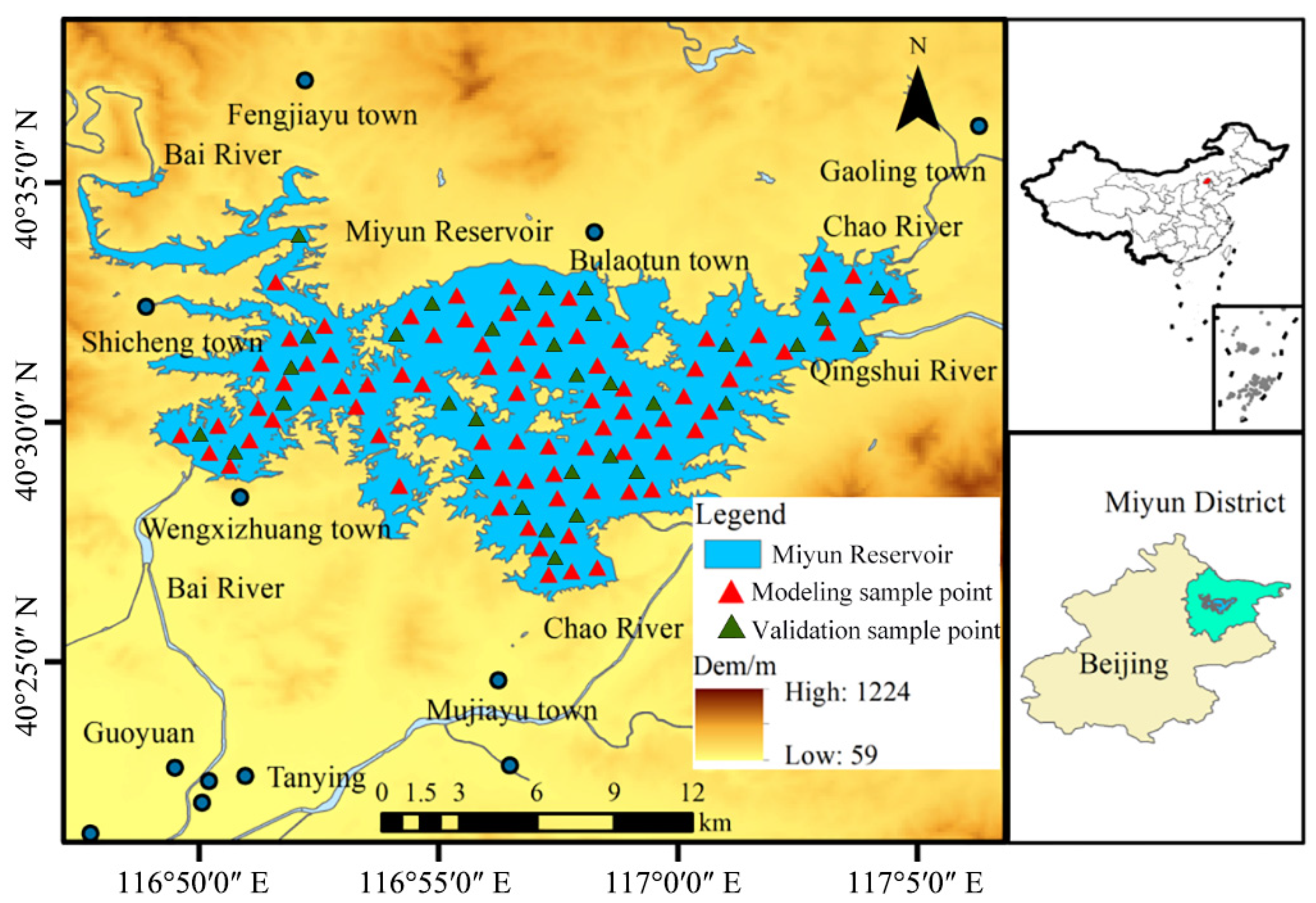
2.1. Study Area

Miyun Reservoir is located in the northeast part of Beijing and among the mountainous area of Yanshan (Figure 1). It was built in 1960 and was the largest reservoir in north China. The study area has a temperate semi-humid monsoon climate with an annual average temperature of 10 °C and annual precipitation of 665 mm. The precipitation is concentrated in the flood season, and the surface runoff formed by precipitation is the main supply source for this reservoir. The upstream of Miyun Reservoir has a fragile ecological environment and serious soil erosions, which can cause soil surface destruction, soil fertility decline, and channel silt deposition [26]. At the same time, water as a carrier brings considerable nitrogen, phosphorus, and other nutrients to the downstream water body, resulting in excessive pollutants in this reservoir. Although exploitation and use of water and soil resources are strictly restricted in the Miyun area to protect Miyun Reservoir and its surrounding environment, social and economic activities still have considerable impacts on the surrounding environment of the reservoir and pose a certain threat to the drinking water supply of this reservoir [27].

2.2. Data Sources and Processing

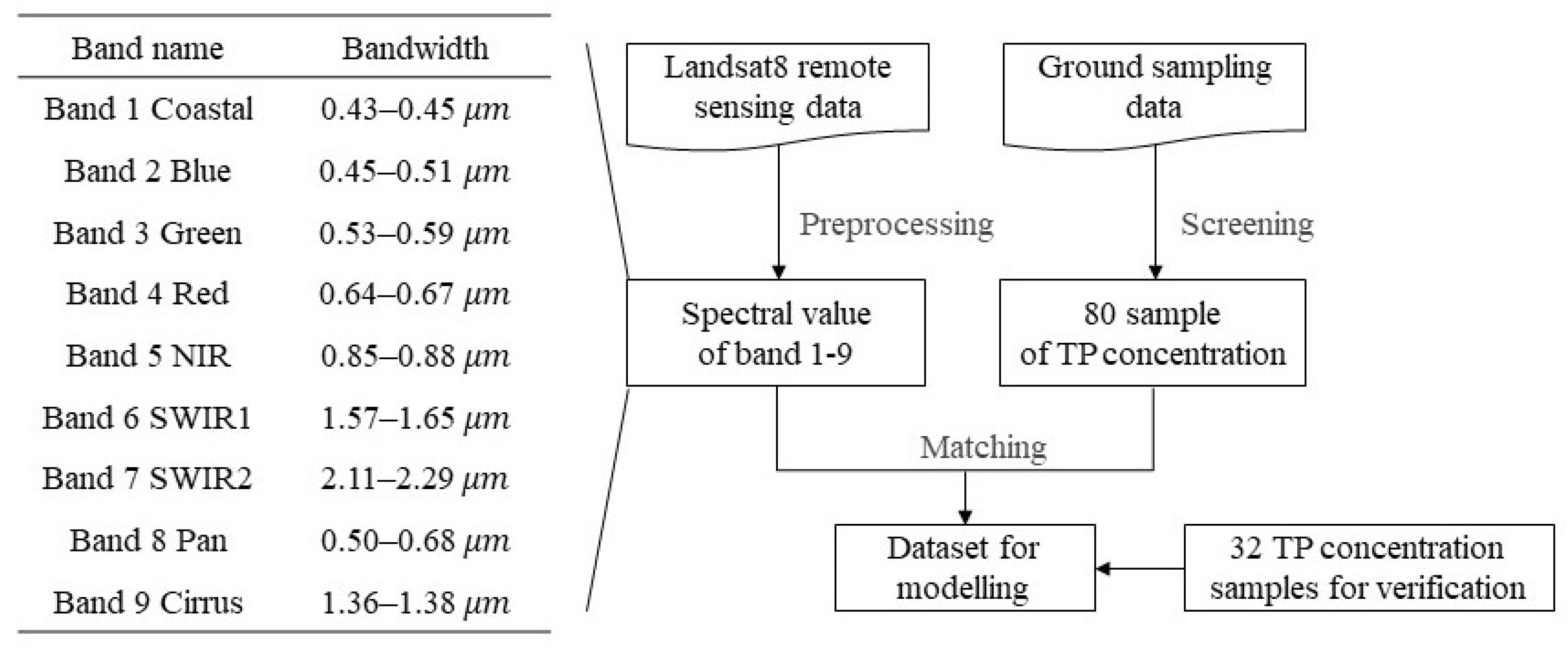
2.2.1. Remote Sensing Data

The Landsat 8 OLI_TIRS data used in this study was from the USGS website (https://earthexplorer.usgs.gov/ accessed on 15 September 2019). Since Landsat 8 L1 T files had been topographically corrected, the coordinate accuracy can basically meet the requirements of small and medium-size scale applications [28,29]. In this study, 24 scenes of Landsat 8 OLI_TIRS data from April 2018 to March 2019 were selected. The radiometric correction was performed by obtaining orthographic parameters in metadata by using the Apply Flash Setting tool, and the radiometric calibration was tuned with the radiometric calibration tools.

2.2.2. Ground Monitoring Data

In this study, 80 water samples were collected in the study area in October 2018 for the retrieval model of TP concentration. In addition, another 32 water samples were collected in April and July 2019 to verify the accuracy of the model, as shown in Figure 1, all of which were taken from a depth of 0–20 cm. The TP concentration measurement was in accordance with the GB/T 1893–1989 standard. The potassium persulfate was used as the oxidant, and then the unfiltered water sample was digested. Finally, ammonium molybdate spectrophotometry was used to measure the TP concentration, which includes the dissolved, suspended, organic, and inorganic phosphorus amounts.

2.2.3. Data Set for Modeling
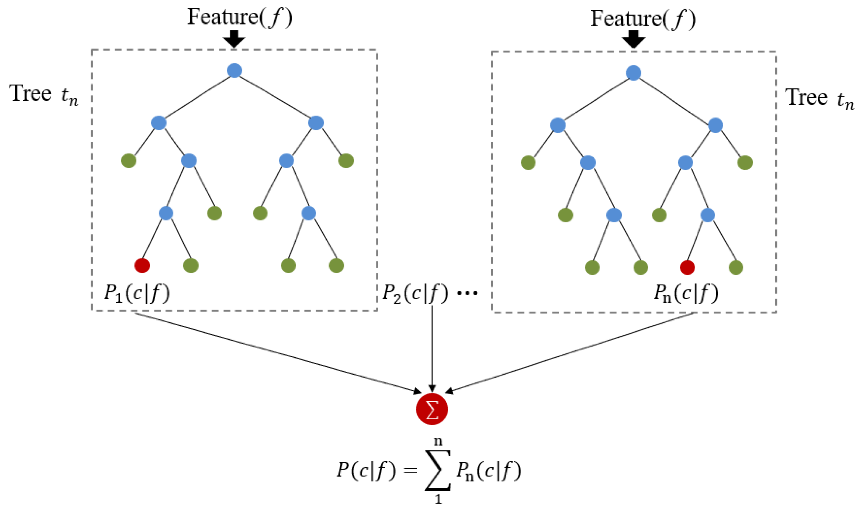
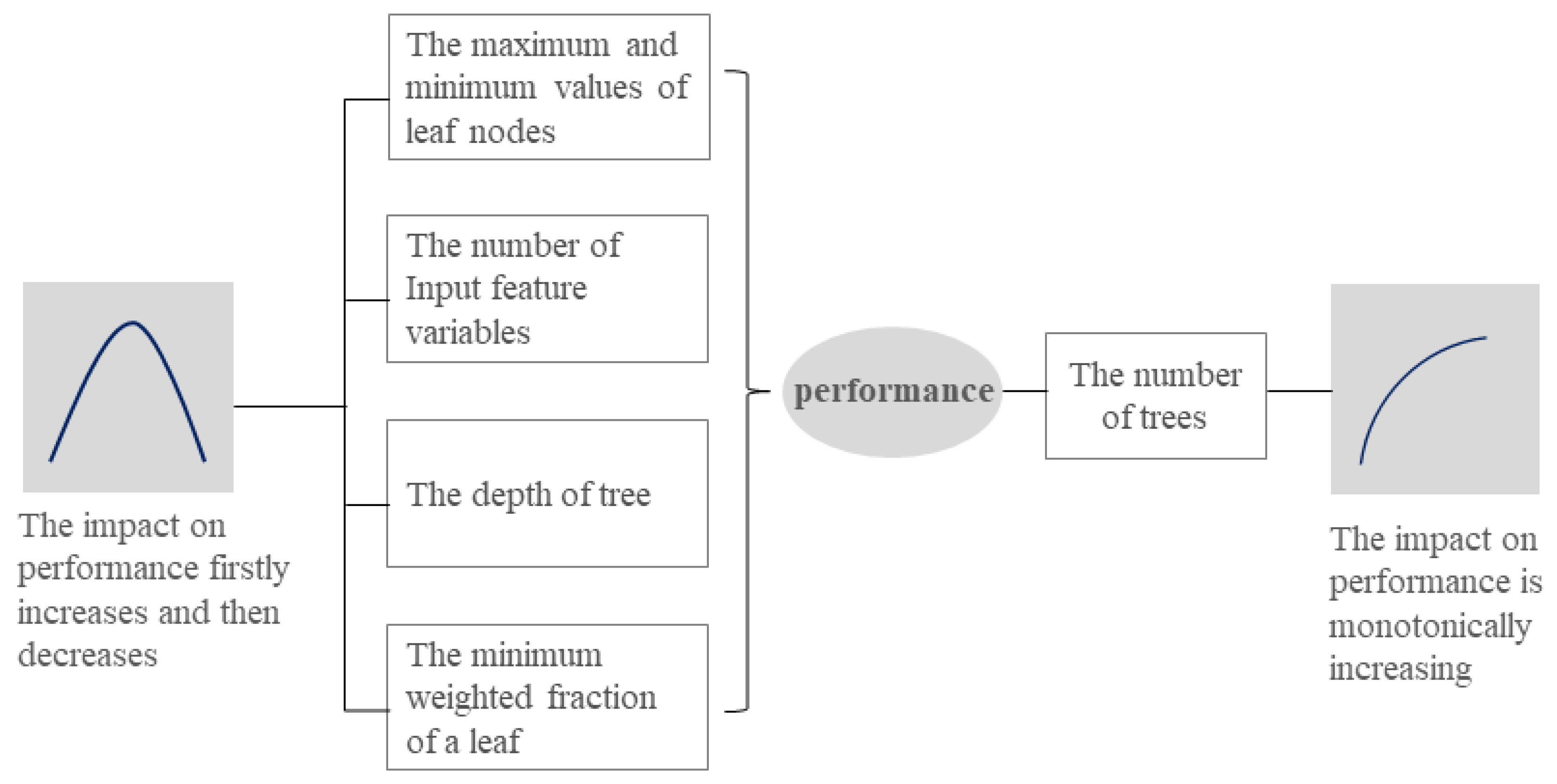
The spectral values of nine bands of Landsat8 remote sensing data were extracted, including coastal band, three visible bands, near-infrared band, two short-wave infrared bands, panchromatic band, and Cirrus band (Figure 2). After the spatial overlaying for the ground sampling data and 9 bands data of Landsat8 remote sensing images, the data set for modeling was extracted from the 9 bands in 80 points corresponding to the ground sampling points. Among these, the spectral value of nine bands was taken as the input training data, while the ground sample data of TP concentration were taken as the target output data. Finally, the retrieval model of TP concentration was built based on the data set for modeling.

2.3. Methods

This study used twelve machine learning algorithms, including support vector machine (SVM), artificial neural network (ANN), Bayesian ridge regression (BRR), lasso regression (Lasso), elastic net (EN), linear regression (LR), decision tree regression (DTR), K neighbor regression (KNR), random forest regression (RFR), extra trees regression (ETR), AdaBoost regression (ABR) and gradient boosting regression (GBR), to build the retrieval model of TP concentration and then selected the most suitable one to calculate the TP concentration in Miyun Reservoir. Finally, it was found that the ETR algorithm was the best one for the retrieval of TP concentration. Therefore, the ETR algorithm was described in detail as follows, while the other algorithms, please see Table 1 and the article links: https://doi.org/10.1016/j.ecolind.2021.107356 (accessed on 18 September 2021) [29,30,31,32,33,34,35,36,37,38,39,40,41,42,43,44,45,46,47,48,49,50,51,52,53,54,55,56,57,58,59,60,61,62,63,64,65,66,67,68].
Where n is the number of samples, p is the sample dimension, m is the number of features, k is the number of hidden layers, i is the number of iterations, o is the output feature, h is the number of neurons, and t is the number of trees.
The ETR algorithm was a typical algorithm for the bagging series. The final results can be obtained by voting or averaging on the basis of combining several weak learners so that the model has high precision and generalization ability [56]. The ETR established each decision tree by using all training samples, i.e., each decision tree originates from the same training sample collection. Moreover, the ETR used just one attribute to achieve the purpose of bifurcation [57]. The principle can be described as follows.
There were n samples randomly selected from the original input data set to obtain a training set, and the rest were used as test data sets. It was assumed that m random decision trees were generated in total.
D = { ( x 1 , y 1 ) , ( x 2 , y 2 ) , , ( x N , y N ) }
where D refers to the training data set, x is the input variable, and y is the output variable.
In the process of training a CART decision tree, the rule of sharding for each node is to first randomly select K features from all features and then select the optimal sharding point from these K features to make the division of left and right subtrees (Figure 3).
Step 1: Choose the optimal splitting variable j and the cut point s to divide the left and right subtrees. There are multiple feature variables, which are divided into binary trees. The optimal segmentation variable j is the feature variable with the smallest partition error. The cut point s is the optimal threshold of the left and right subtrees, namely the node corresponding to the optimal segmentation variable.
m i n j , s [ m i n c 1 x i R 1 ( j , s ) ( y i c 1 ) 2 + m i n c 2 x i R 2 ( j , s ) ( y i c 2 ) 2 ]
where j is the splitting variable, s is the cut point, and c is the output value of each sub-intervals. Both R 1 and R 2 are the intervals that are divided, and y is the output variable.
Step 2: The selected ( j ,   s ) value is used to divide the feature space. In the ETR algorithm, each selected feature variable is random; therefore, the above steps were repeated until the corresponding sample number of all leaf nodes was less than or equal to m m i n .
Step 3: Integrate all the decision trees, and the average method is used to determine the final regression model. y m is used to represent the set of m decision trees and the test data set T is used to verify one by one, and the average synthesis of m decision trees is carried out according to the verification results.
f ( x ) = y m ¯ = 1 n i = 1 n y m i
where f ( x ) is the final regression model and y m represents each decision tree.
As for the hyper-parameters, the more the number of random decision trees, the better the model performance. The influence of the number of leaf nodes and feature number on the algorithm performance will increase first and then decrease (Figure 4) [58]. Through repeated testing, a set of appropriate hyper-parameters is set for the algorithm. The number of trees was 125, and the maximum depth of the tree was set as 25 to improve the efficiency of the operation, while the rest of the parameters took default values.

3. Results

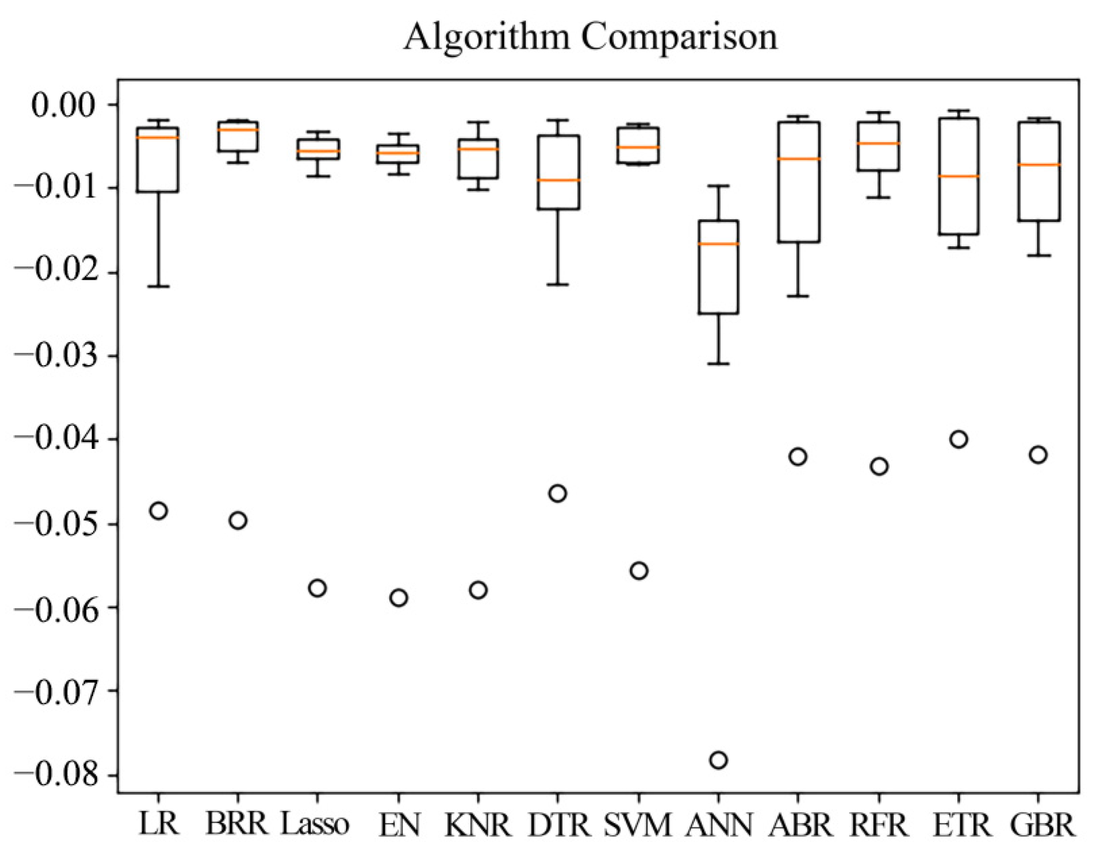
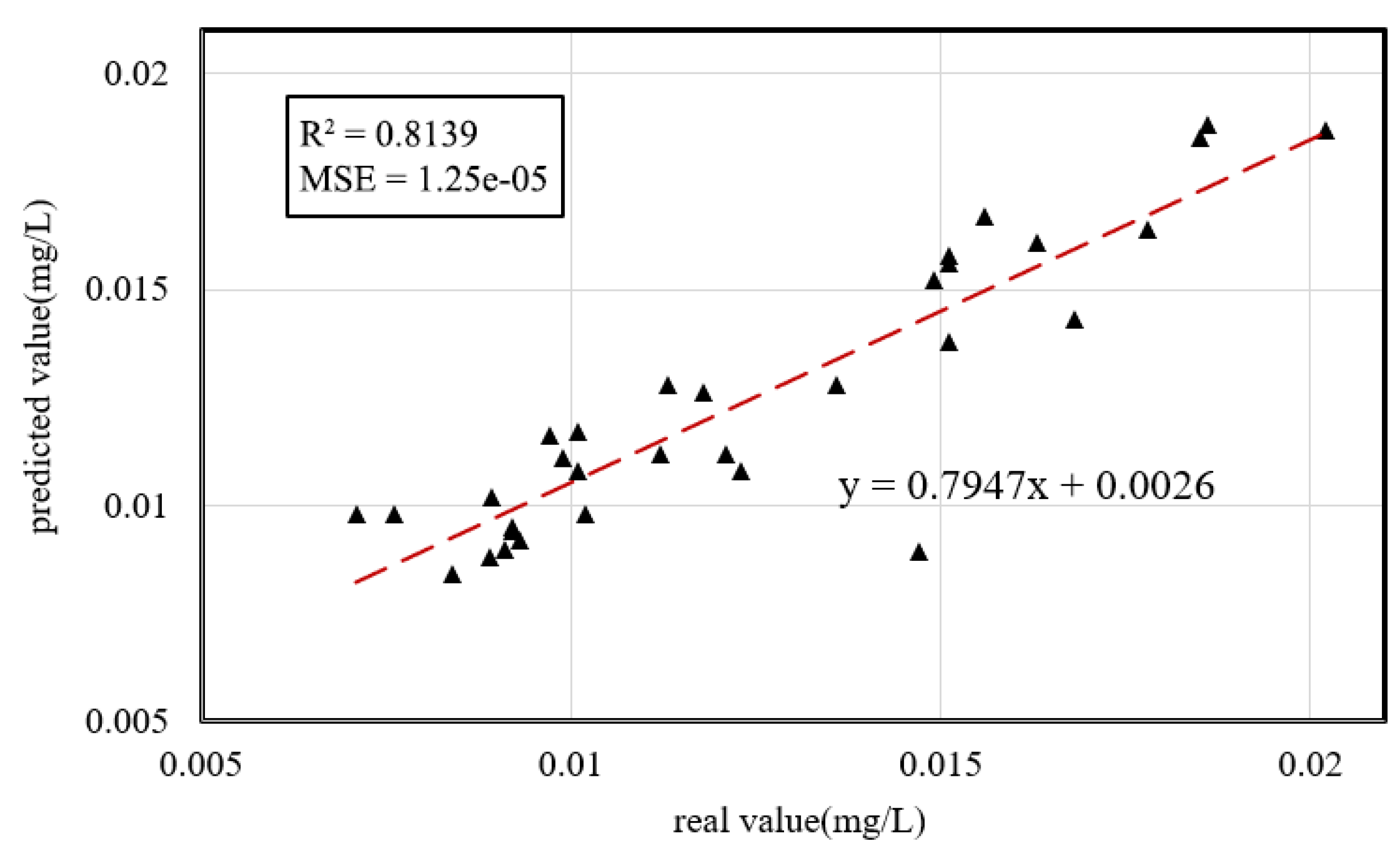
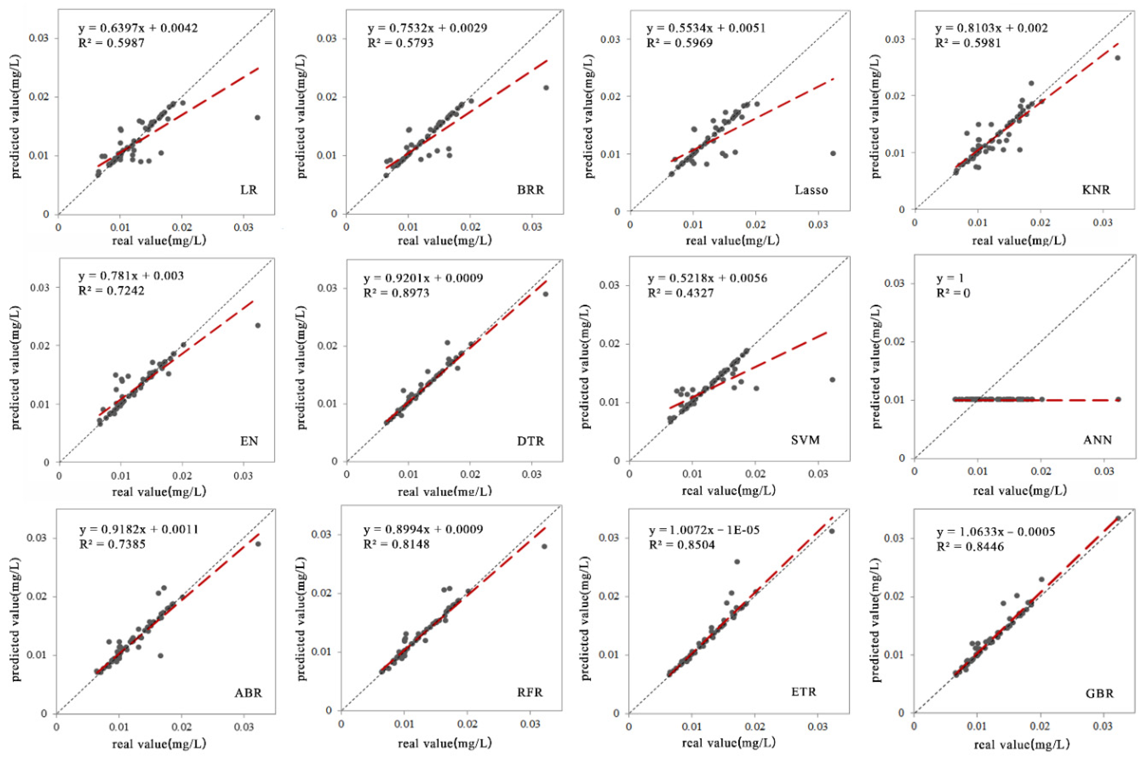
3.1. Retrieval Modeling and Validation for the TP Concentration

The machine learning algorithms were very sensitive to the input data set; thus, this study firstly analyzed the model performance by the mean squared error (MSE) regression loss based on the input data set and the K-fold cross-validation [37]. The 10-fold cross-validation was used to evaluate the accuracy of 12 machine learning algorithms. It divides the sample data set into 10 subsets, 9 of them were taken as the training data, and the remaining 1 was taken as the testing data. After 10 rounds of modeling, the average error was calculated to evaluate the accuracy of these models [38]. It can avoid using the same experimental data to test the model and represent the average accuracy of the retrieval model of TP concentration. As seen from Figure 5, the negative value of MSE was used as the evaluation criterion in Scikit-learn. The distribution of MSE of two algorithms of ETR and GBR were relatively centralized, with a small gap between the upper and lower limits. The median value was around 0.01, which was close to the middle part, indicating that the distribution of MSE was relatively stable and had suitable performance. It should be considered as the key modeling algorithm. In addition, the rationality of the ABR and DTR algorithms was also higher than other algorithms. The abnormal value of the ANN algorithm was extremely large, and its gap between the upper and lower limits was also large; thus, the ANN algorithm was not ideal for retrievals of TP concentration.
Based on the ground monitoring data and Landsat8remote sensing data, 12 machine learning models were used to establish the retrieval model for the TP concentration in Miyun Reservoir. The retrieval model was built in the Python environment, and the arcpy library function was used to perform basic processes such as format conversion and mask extraction on the remote sensing data. In this study, the integrated data set including spectral information and ground sampling data of 80 sampling sites was used as the input data set, and then the data set was separated. During the training process, it was found that when the random seed was set as 7, the best results can be obtained. The input data set was converted into a one-dimensional array based on the numpy library, the basic models of 12 machine learning algorithms were loaded through the sklearn library, and the library pickle was used to deploy the retrieval results. Thereafter, the retrieval results were reconverted into the array format associated with the header file and then were reconverted into raster format with the arcpy library function. Finally, the retrieval results of the TP concentration in the Miyun Reservoir were obtained. In this model, 80% of the data was selected as the training data set, while 20% was used for the validation.
This study also used the mean absolute error (MAE), the mean square error (MSE), the explained variance score, and the determination coefficient (R2) to assess the model performance (Table 2). Moreover, the comparison of the ground monitoring data and the corresponding modeling results were offered in Figure 6 to visualize the model fit. As it was seen from Figure 6, the worst performance was obtained with the ANN model. The fitting curve was approximately a straight line indicating that the single-layer network model was not applicable to the sample data and it was not sensitive to the TP concentration obtained from the field. Comparatively speaking, the models of Lasso, LR, KNR, BRR, and SVM algorithms can achieve a certain degree of fitting, while the models of DTR, ETR, GBR algorithms obtained the maximum fitting values for the input original data set (Figure 6 and Table 2).
As seen from the assessment parameters of model performance, the two best-performing algorithms were obtained to be DTR and ETR with the R2 values higher than 0.85, the MAE lower than 0.000433 mg/L, and MSE lower than 0.000003 mg/L. Then it was followed by the GBR and RFR with the R2 of 0.844646 and 0.814851, respectively (Table 1). It meant that the fits were representative of the ground monitoring data by 84.5% and 81.5%, respectively. For other algorithms, the fitting degree was lower. Although the assessment parameters of DTR and ETR were both excellent, this study selected the ETR. Because the distribution of the MSE of the ETR algorithm was more centralized than that of the DTR algorithm, what is more, the ETR algorithm was an integration of the DTR algorithm. Therefore, the ETR algorithm was chosen as the retrieval model of the TP concentration to be performed in the study area.

3.2. Retrieval Results of the TP Concentration and Its Water Quality Evaluation in Miyun Reservoir

3.2.1. Accuracy Verification of the Retrieval Model

To further validate the accuracy and stability of the retrieval model for the TP concentration, this study used the ground monitoring data of TP concentration in another 32 sampling points, which were not included in the modeling sample, to verify the accuracy of the model. The results showed that the retrieval model based on the ETR algorithm had great accuracy with R2 of 0.813927, MSE of 0.0000125. The fitting scatter plot was shown in Figure 7, which also indicated that the ETR algorithm can accurately achieve the retrieval for the TP concentration.

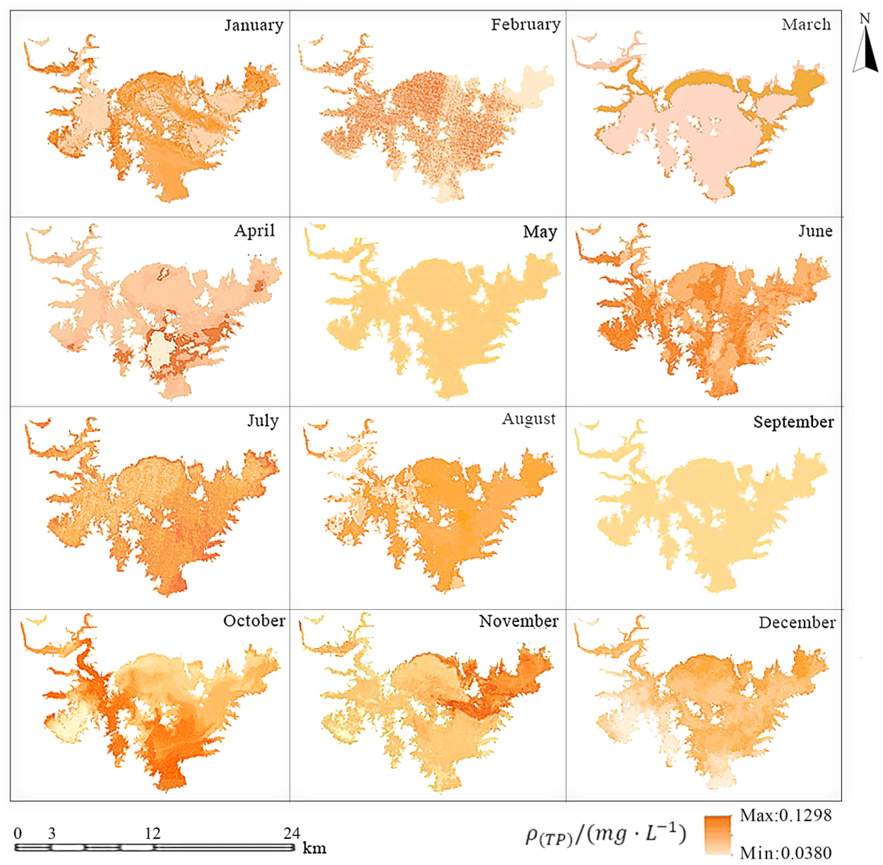
3.2.2. Spatio-Temporal Evolution of the TP Concentration in Miyun Reservoir

Based on the model built by using the ETR algorithm, the TP concentration variation over the Miyun Reservoir was estimated at pixel level from April 2018 to March 2019. The spatial distribution of TP concentration was provided on a monthly basis to analyze their spatial-temporal evolution in Figure 8. The results showed that the fluctuation of TP concentration was relatively high on a monthly basis. In April, the maximum TP concentration value was 0.0662 mg/L while the minimum was 0.0632 mg/L, and the TP concentration with a high value was observed to be in the southeast of the reservoir while it was lower in the north and west. In May, the TP concentration decreased to a certain degree, and its maximum value was 0.0646 mg/L, which was lower than that in April. On the other hand, the minimum value increased to 0.0644 mg/L, and it indicated that the TP concentration tended to be almost stable in the whole reservoir area for this month.
In June, the TP concentration fluctuation was relatively high, with a maximum value of 0.0751 mg/L and a minimum value of 0.0554 mg/L. High-concentration areas appeared in the west of the reservoir, which was near the tributaries of Miyun Reservoir, and the pollutant migrated by tributary runoff or rainfall was the possible reason for this. The fluctuation in June occurred in the west, spread to the east, and finally converged to the east edge of the reservoir in July. The TP concentration in July seemed to be varying from the maximum value of 0.0749 mg/L and the minimum value of 0.0561 mg/L. The high-concentration areas were all distributed in the tributaries area or on the northeast edge of the reservoir.
The overall concentration variation decreased in August by observing a maximum value of 0.0704 mg/L and a minimum value of 0.0622 mg/L. Relatively lower concentrations were distributed in the east, and it showed an overall increasing trend from east to west compared to July. In September, the maximum value of the concentration gradually dropped to 0.066 mg/L while the minimum value was 0.0622 mg/L. It indicated that a very small regional variation occurred in this month. In October, the maximum value of TP concentration increased sharply to 0.1298 mg/L while the minimum value dropped to 0.0380 mg/L. Starting in October, the concentration fluctuated frequently. It firstly spread inward from the west and south and then increased in the northeast in November.
The TP concentration increased again after late December, especially the increase that occurred in the north and northeast. It reached a peak again in January. Although the TP concentration gradually fell back in February, the concentration in the whole reservoir was still high. In March, the TP concentration decreased in the center area due to the ice melting, while a new concentration increase occurred at the edge of the reservoir, mainly on the north and east coasts.

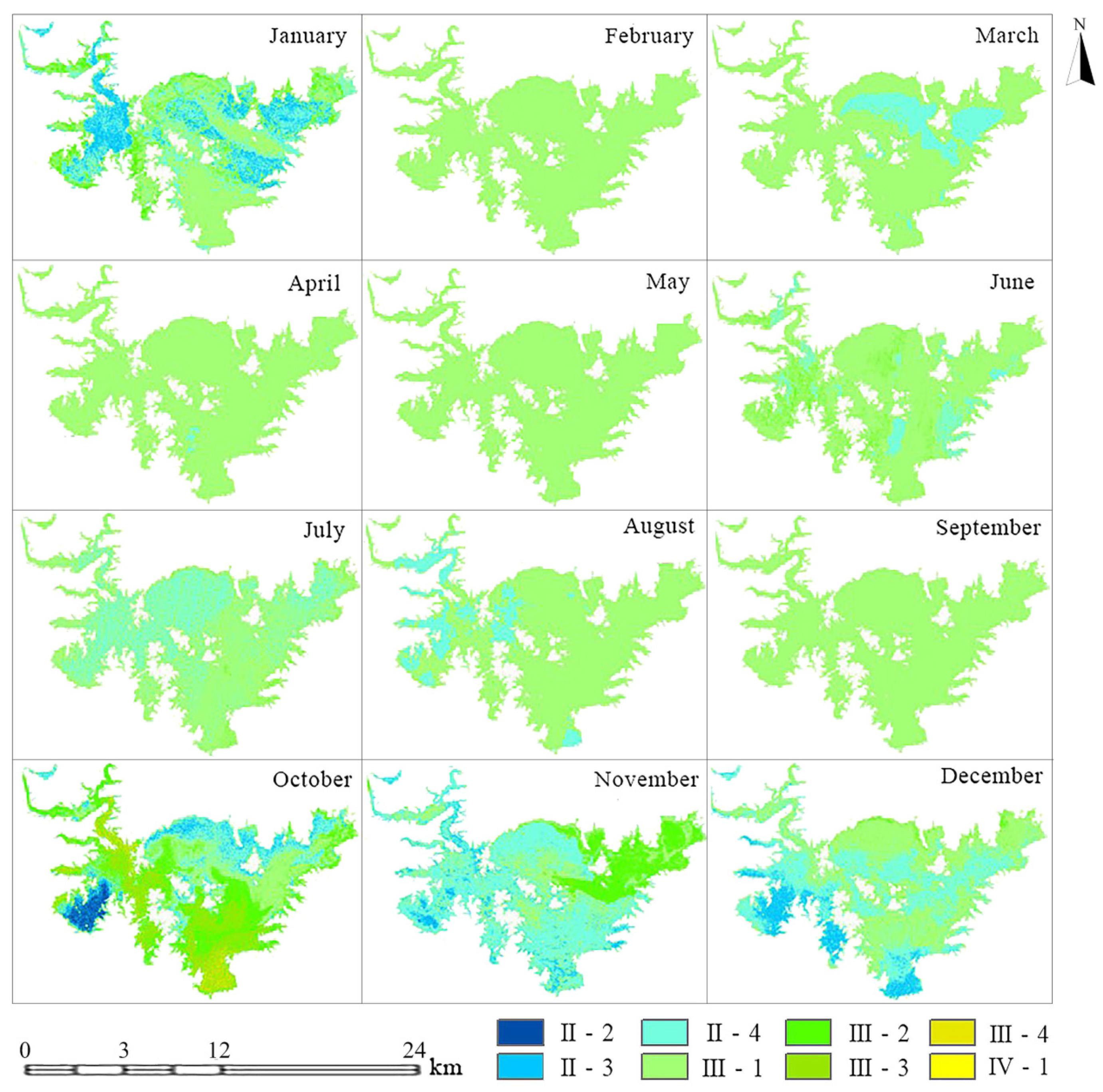
3.2.3. Water Quality Assessment Based on Surface Water Environmental Standards

In accordance with the Environmental Quality Standard for Surface Water GB3838-2002, the range of retrieval results was compared with the standard limit value of basic items of Environment Quality Standard for surface water. The standard limit required the TP concentration to be calculated by the amount of phosphorus element. However, the phosphorus concentration obtained in the water quality measurement in this study was the PO 4 3 concentration. Therefore, the concentration amounts should be multiplied by the coefficient of 0.392, which was obtained from p/(p + 4O).
The standard limit values of the TP concentration in GB3838-2002 (SEPA, 2002) were provided in Table 3. The distribution range of each class in this study was determined by reclassifying the retrieval results of TP concentration. Due to the TP concentration in Miyun Reservoir were mainly centered at the ranges of only one or two levels, each class was equally subdivided into four intervals by the method of [(standard limit value of level I, the standard limit value of level I + (standard limit value of level I + 1 standard limit value of level I) ∗ (0.25 | 0.5 | 0.75 |1)] in order to better explore the change in the TP concentration.
According to the equal interval classification, the standard limit value of TP concentration was divided into 12 categories, namely II-1, II-2, II-3, II-4, III-1, III-2, III-3, III-4, IV-1, IV-2, IV-3, and IV-4. According to the TP concentration amounts obtained in this study, the reclassification of the data was grouped into eight classes. The classification results of the TP concentration in the Miyun Reservoir were offered in Figure 9 on a monthly basis.
As a whole, the water quality level in most of the water areas was classified with the level of III-1 from April to May in 2018, and the water quality in the northwest of the reservoir had been switched to class II from June to August. However, most of the areas were labeled as III-1 in September. From October 2018 to January 2019, the water quality showed an improving trend from the southwest and the north, especially near the Bai River dam, where the water quality was classified as II-2. During the period of November and December, the water quality was gradually getting better for most of the regions. On the other hand, there were also some regions where it became worse and were labeled as class III-2. The betterment of water quality areas began to decrease until the following January in 2019, and the improved areas were concentrated mainly in the east and west of the reservoir. The water quality returned to class III-1 until the following year in February. However, the water quality in the north of the reservoir showed an improving trend to class II in March 2019.

4. Discussion

4.1. Water Quality Evaluation Base on the Retrieval Model of TP Concentration

Water quality monitoring was particularly important in water environment management, and the TP concentration was one of the most commonly used indicators. In this study, we compared 12 machine learning algorithms to establish the retrieval model of TP concentration in the Miyun Reservoir. The results showed that DTR, ETR, RFR, and GBR algorithms can achieve high precision retrieval of water quality parameters. It meant that the machine learning algorithms can better establish the functional relationship between spectral information and TP concentration [68,69] as it has strong nonlinear mapping capability ability, fault tolerance, and learning capability [19,20]. Compared with other machine learning methods [70,71,72,73,74,75,76], the ETR and DTR used in this study have relatively small errors. The explained variance scores were above 0.85, and their MSE were lower than 0.000433 mg/L and MSE lower than 0.000003 mg/L. What is more, their fitting performances were better than the other algorithms. Considering the mean squared error regression loss of ETR and DTR, the ETR was chosen for the retrieval model of TP concentration in this study. Compared with the retrieval model (R2 = 0.685) established by Xu et al. [62], the ETR model used in this study had higher accuracy and wider applicability. As the ETR took all the original training data sets as the training samples and randomly selected features, which made the retrieval model more accurate, and the results had better generalization ability [67]. In addition, the retrieval results based on the remote sensing data can realize large-area grid-scale simultaneous observations in Miyun Reservoir [68]. It effectively avoids the area limitation of unmanned aerial vehicles (UAV) due to its short flight time and can fully understand the characteristics of the temporal and spatial evolution in the whole reservoir. However, sometimes it is also limited due to the lower spatial resolution in the study of higher-precision [69].
Then this study explored the spatio-temporal variation of the TP concentration in Miyun Reservoir from April 2018 to March 2019. It can be found that the TP concentration showed a decreasing trend in April, the first fluctuation started from the west of the reservoir in June and converged to the east of the reservoir in July, finally fell back to be stable in September, and the study of Qiu et al. [63] on the TP pollutant load of Miyun Reservoir confirmed this law. The TP concentration migration in June may be caused by the runoff erosion during the flood season, which brought the upstream pollutants into the reservoir. On the one hand, rainwater during the flood season supplemented the water source of the reservoir. On the other hand, it also brought about the expansion of the pollution area. Therefore, it is urgent to carry out small watershed management, improve the vegetation coverage, reduce surface runoff erosion and reduce the phosphorus load into the reservoir due to soil erosion. The second fluctuation of TP concentration occurred in October, which started in the southwest and spread to the northeast, then decreased until January and increased again in March. This is basically consistent with the study of Zhang et al. [64]. There were a number of villages and towns in these two areas, frequent human activities, such as fishery, agriculture, and other activities, have aggravated water pollution and caused TP pollutants to accumulate within a certain range in a short period of time. Therefore, it is necessary to carry out special water quality optimization work for the management of living and agricultural sources in the watershed near villages and towns, the use of chemical fertilizers and pesticides should be further reduced, and sewage discharge is strictly prohibited, and then the water pollution will be reduced through cleaner production.
In addition, this study classified the water quality in Miyun Reservoir based on the Environmental Quality Standard for Surface Water GB3838-2002. The results showed that the water quality of Miyun Reservoir represented by TP concentration was at the level of III-1 most of the time, and it improved slightly in March, June, July, and August and reached a level of II in the southwest of the reservoir. This is due to the long-term protection of the Miyun Reservoir, Although the concentration of pollutants has been concentrated in some areas since June, the water quality in other areas has improved significantly, and the overall water quality level has been improved. The regional variation of water quality became obvious in October. The water quality in the west of the reservoir was improved significantly to II-2, but in the northeast was deteriorated to III-2, then it leveled off in the following February. This is consistent with the results conducted by Qin et al. [65] and Gang et al. [66]. On the whole, surface pollution was prominent during the flood season, and non-flood season point source pollution was the dominant factor, which showed that the runoff caused by rainfall was an important reason for the deterioration of water quality. The reason that the water quality in the southwest of the reservoir was generally better than in the northeast may be related to pollution emissions from the human activities in the upstream to the northeast area, such as free-range poultry and near-shore farming. Therefore, water quality protection and monitoring in the upper and middle reaches of Miyun Reservoir can not be ignored. Due to the limited self-purification capacity of the water body, some pollutants will be adsorbed in the bottom mud. When the water velocity increases, the pollutants in the bottom mud will be released again. Therefore, the discharge of different pollution sources in the river basin should be controlled.

4.2. Limitation in the TP Concentration Retrieval Model

Although the accuracy of the total phosphorus concentration retrieval model built in this study for Miyun Reservoir had met the requirements, there were still some shortcomings to be further explored. Firstly, the number of ground monitoring sampling data used in this study was 80, which were collected during the same period, while no multi-phase data were collected. However, the water quality parameters in Miyun Reservoir significantly varied with time and space. Therefore, more long-time data would be useful for further improvement of the model, and more accumulated ground data would contribute to a more accurate retrieval model and realistic analysis. Additionally, the integration of multi-period historical data and other ancillary data can be used as validation data to support the model’s reliability. For example, flood information, planting information, etc., can influence the change of pollutant concentration so that they should be considered while constructing the retrieval model to have a better model accuracy.

5. Conclusions

In this study, Landsat 8 remote sensing data and ground monitoring data were used to build a more accurate retrieval model for the TP concentration in the Miyun Reservoir by comparing 12 machine learning algorithms. The performance of 12 machine learning algorithms was assessed and compared by using the MSE, the explained variance score, the determination coefficient R2 and the fitting line. It was concluded that the ETR was the most accurate and suitable algorithm for the retrieval model of TP concentration. Afterward, the TP concentration was estimated at pixel level by the built retrieval model, and the spatial-temporal evolution and assessment of water quality were explored. The results showed that the TP concentration in Miyun Reservoir was between 0.0380 and 0.1298 mg/L, but it fluctuated from June to July and October to the following January, and this is consistent with the results of a study by Zhang et al. [64] at the same time. The fluctuations generally occurred along the west side of Miyun Reservoir, then spread to the center, showing a trend of gathering to the northeast bank. Moreover, TP concentration in summer was lower than that in other seasons, and TP concentration in the southwest part of the reservoir was generally lower than in the northeast, as there was less human activities interference. The water quality was generally safe in line with the Environmental Quality Standard for the surface water environment, except only an over-standard case occurrence in the spring and September. These conclusions could provide a scientific reference for water monitoring and water management in Miyun Reservoir.

Author Contributions

Q.J., Z.Q. and S.S. designed the conceptual model study and aim; Z.Q. contributed to the model development and prepared the manuscript; Q.J. revised the manuscript; L.X. prepared modeling data sets; Y.W. and H.Y. contributed to results interpretation. All authors have read and agreed to the published version of the manuscript.

Funding

This research was funded by the National Science and Technology Projects (no. 2017ZX07108002 and no. 2017ZX07101004), the National Natural Science Foundation of China (no. 41901234, no. 51909052 and no. 41807169), and the Natural Science Foundation of Hebei Province (E2019403210), Science and Technology Project of Hebei Education Department (BJ2019045).

Institutional Review Board Statement

Not applicable.

Informed Consent Statement

Not applicable.

Data Availability Statement

The landsat8 remote sensing data can of this study are openly available at http://www.gscloud.cn/sources/ accessed on 18 September 2021.

Acknowledgments

This research was supported by the National Science and Technology Projects (no. 2017ZX07101004 and no. 2017ZX07108002), the National Natural Science Foundation of China (no. 41901234, no. 51909052 and no. 41807169), and the Natural Science Foundation of Hebei Province (E2019403210), Science and Technology Project of Hebei Education Department (BJ2019045). Data support from projects of the National Natural Science Foundation of China (no. 71225005) and the Exploratory Forefront Project for the Strategic Science Plan in IGSNRR, CAS is also appreciated. In addition, we gratefully acknowledge the Beijing Municipal Education Commission for their financial support through the Innovative Transdisciplinary Program “Ecological Restoration Engineering”.

Conflicts of Interest

The authors declare that they have no known competing financial interests or personal relationships that could have appeared to influence the work reported in this manuscript. The manuscript entitled “Retrieval of Total Phosphorus Concentration in the Surface Water of Miyun reservoir based on Remote Sensing Data and Machine Learning Algorithms”.

References

  1. Al-Jawad, J.Y.; Alsaffar, H.M.; Bertram, D.; Kalin, R.M. A comprehensive optimum integrated water resources management approach for multidisciplinary water resources management problems. J. Environ. Manag. 2019, 239, 211–224. [Google Scholar] [CrossRef]
  2. Yu, Q.; Jiang, Q.; Yang, D.; Yue, D.; Ma, H.; Huang, Y.; Zhang, Q.; Fang, M. Incorporating Temporal and Spatial Variations of Groundwater into the Construction of a Water-Based Ecological Network: A Case Study in Denko County. Water 2017, 9, 864. [Google Scholar] [CrossRef] [Green Version]
  3. Kumar, P.; Liu, W.; Chu, X.; Zhang, Y.; Li, Z. Integrated water resources management for an inland river basin in China. Watershed Ecol. Environ. 2019, 1, 33–38. [Google Scholar] [CrossRef]
  4. Venkatesh, A.; Roopa, D. Assessment of Ground Water Quality in Thuraiyur Taluk Namakkal District. Int. J. Civ. Eng. 2020, 7, 30–34. [Google Scholar] [CrossRef]
  5. De Vitry, M.M.; Kramer, S.; Wegner, J.D.; Leitão, J.P. Scalable flood level trend monitoring with surveillance cameras using a deep convolutional neural network. Hydrol. Earth Syst. Sci. 2019, 23, 4621–4634. [Google Scholar] [CrossRef] [Green Version]
  6. Haghiabi, A.H.; Nasrolahi, A.H.; Parsaie, A. Water quality prediction using machine learning methods. Water Qual. Res. J. Can. 2018, 25, 23–28. [Google Scholar] [CrossRef]
  7. Rozpondek, K.; Rozpondek, R.; Pachura, P. Characteristics of spatial distribution of phosphorus and nitrogen in the bottom sediments of the water reservoir. J. Ecol. Eng. 2017, 18, 178–184. [Google Scholar] [CrossRef]
  8. Huang, C.; Zhang, Y.; Huang, T.; Yang, H.; Li, Y.; Zhang, Z.; He, M.; Hu, Z.; Song, T.; Zhu, A.-X. Long-term variation of phytoplankton biomass and physiology in Taihu lake as observed via MODIS satellite. Water Res. 2019, 153, 187–199. [Google Scholar] [CrossRef] [PubMed]
  9. Chapman, D.V.; Bradley, C.; Gettel, G.M.; Hatvani, I.G.; Hein, T.; Kovács, J.; Liska, I.; Oliver, D.M.; Tanos, P.; Trásy, B.; et al. Developments in water quality monitoring and management in large river catchments using the Danube River as an example. Environ. Sci. Policy 2016, 64, 141–154. [Google Scholar] [CrossRef] [Green Version]
  10. Wimmer, A.; Markus, A.A.; Schuster, M. Silver Nanoparticle Levels in River Water: Real Environmental Measurements and Modeling Approaches—A Comparative Study. Environ. Sci. Technol. Lett. 2019, 11, 32–38. [Google Scholar] [CrossRef]
  11. Ryberg, K.R.; Blomquist, J.D.; Sprague, L.A.; Sekellick, A.J.; Keisman, J. Modeling drivers of phosphorus loads in Chesapeake Bay tributaries and inferences about long-term change. Sci. Total Environ. 2017, 1423, 616–617. [Google Scholar] [CrossRef]
  12. Lai, Y.; Zhang, J.; Song, Y.; Gong, Z. Retrieval and Evaluation of Chlorophyll-a Concentration in Reservoirs with Main Water Supply Function in Beijing, China, Based on Landsat Satellite Images. Int. J. Environ. Res. Public Health 2021, 18, 4419. [Google Scholar] [CrossRef]
  13. Wang, Y.; Jiang, Y.; Liao, W.; Gao, P.; Huang, X.; Wang, H.; Song, X.; Lei, X. 3-D hydro-environmental simulation of Miyun reservoir, Beijin. HydroResearch 2014, 8, 383–395. [Google Scholar] [CrossRef]
  14. Neil, C.; Spyrakos, E.; Hunter, P.; Tyler, A. A global approach for chlorophyll-a retrieval across optically complex inland waters based on optical water types. Remote Sens. Environ. 2019, 229, 159–178. [Google Scholar] [CrossRef]
  15. Sayers, M.J.; Bosse, K.R.; Shuchman, R.A.; Ruberg, S.A.; Fahnenstiel, G.L.; Leshkevich, G.A.; Stuart, D.G.; Johengen, T.H.; Burtner, A.M.; Palladino, D. Spatial and temporal variability of inherent and apparent optical properties in western Lake Erie: Implications for water quality remote sensing. J. Great Lakes Res. 2019, 45, 490–507. [Google Scholar] [CrossRef]
  16. Wang, X.; Xiao, C.; Xue, Z.Y.; Pu, Q.C.; Jiang, T.; Zhao, J.H.; Wang, S.M. Application of Remote Sensing Technology to Monitor NH3N Distribution in the Danjiangkou Reservoir. J. Water Resour. Res. 2019, 8, 436–444. [Google Scholar] [CrossRef]
  17. Yao, J.; Meng, D.; Zhao, Q.; Cao, W.; Xu, Z. Nonconvex-Sparsity and Nonlocal-Smoothness-Based Blind Hyperspectral Unmixing. IEEE Trans. Image Process. 2019, 28, 2991–3006. [Google Scholar] [CrossRef]
  18. Hong, D.; Gao, L.; Yao, J.; Zhang, B.; Plaza, A.; Chanussot, J. Graph Convolutional Networks for Hyperspectral Image Classification. IEEE Trans. Geosci. Remote Sens. 2020, 59, 5966–5978. [Google Scholar] [CrossRef]
  19. Liu, J.; Zhang, Y.; Yuan, D.; Song, X. Empirical Estimation of Total Nitrogen and Total Phosphorus Concentration of Urban Water Bodies in China Using High Resolution IKONOS Multispectral Imagery. Water 2015, 7, 6551–6573. [Google Scholar] [CrossRef] [Green Version]
  20. Chidammodzi, C.L.; Muhandiki, V.S. Water resources management and Integrated Water Resources Management implementation in Malawi: Status and implications for lake basin management. Lakes Reserv. Res. Manag. 2017, 22, 12–19. [Google Scholar] [CrossRef]
  21. Nour, M.H.; Smith, D.W.; El-Din, M.G.; Prepas, E.E. Effect of watershed subdivision on water-phase phosphorus modelling: An artificial neural network modelling application. J. Environ. Eng. Sci. 2008, 7, 95–108. [Google Scholar] [CrossRef]
  22. Sun, D.; Qiu, Z.; Li, Y.; Shi, K.; Gong, S. Detection of Total Phosphorus Concentrations of Turbid Inland Waters Using a Remote Sensing Method. Water Air Soil Pollut. 2014, 225, 1–17. [Google Scholar] [CrossRef]
  23. Gao, Y.; Gao, J.; Yin, H.; Liu, C.; Xia, T.; Wang, J.; Huang, Q. Remote sensing estimation of the total phosphorus concentration in a large lake using band combinations and regional multivariate statistical modeling techniques. J. Environ. Manag. 2015, 151, 33–43. [Google Scholar] [CrossRef] [PubMed]
  24. Ding, C.; Pu, F.; Li, C.; Xu, X.; Zou, T.; Li, X. Combining Artificial Neural Networks with Causal Inference for Total Phosphorus Concentration Estimation and Sensitive Spectral Bands Exploration Using MODIS. Water 2020, 12, 2372. [Google Scholar] [CrossRef]
  25. Du, C.G.; Li, Y.M.; Wang, Q.; Zhu, L.; Lv, H. Inversion model and daily variation of total phosphorus concentrations in Taihu Lake based on GOCI Data. Environ. Sci. 2016, 37, 862–872. [Google Scholar] [CrossRef]
  26. Wang, Y.X.; Yang, G.F.; Lin, M.S.; Yang, S.T. Calculating total phosphorus in reservoirs using the satellite Landsat data. J. Irrig. Drain. Eng. 2017, 36, 105–109. [Google Scholar] [CrossRef]
  27. Hao, W.; Ge-Ping, L.; Wei-Sheng, W.; Konstantin, P.; Yao-Ming, L.; Hong-Wei, Z.; Wei-Jie, H. Inversion of soil moisture content in the farmland in middle and lower reaches of Syr Darya River Basin based on multi-source remotely sensed data. J. Nat. Resour. 2019, 34, 2717–2731. [Google Scholar] [CrossRef]
  28. Ingles, J.; Louw, T.; Booysen, M. Water quality assessment using a portable UV optical absorbance nitrate sensor with a scintillator and smartphone camera. Water SA 2021, 47, 135–140. [Google Scholar] [CrossRef]
  29. Sahoo, S.; Russo, T.A.; Elliott, J.; Foster, I. Machine learning algorithms for modeling groundwater level changes in agricultural regions of the U.S. Water Resour. Res. 2017, 53, 3878–3895. [Google Scholar] [CrossRef]
  30. Huang, L.M.; Chen, B.; Tian, Y.; Huang, N.; Li, N. Coupling relationship optimization of landscape structure and conservation function of lake and reservoir drinking water sources in Nanning, China. Acta Ecol. Sin. 2019, 39, 3494–3506. [Google Scholar] [CrossRef]
  31. Fezzi, C.; Harwood, A.R.; Lovett, A.A.; Bateman, I.J. Erratum: The environmental impact of climate change adaptation on land use and water quality. Nat. Clim. Chang. 2018, 5, 385. [Google Scholar] [CrossRef] [Green Version]
  32. Bai, J.; Shen, Z.; Yan, T.; Qiu, J.; Li, Y. Predicting fecal coliform using the interval-to-interval approach and SWAT in the Miyun watershed, China. Environ. Sci. Pollut. Res. 2017, 24, 15462–15470. [Google Scholar] [CrossRef]
  33. Qiu, J.; Shen, Z.; Chen, L.; Hou, X. Quantifying effects of conservation practices on non-point source pollution in Miyun Reservoir Watershed, China. Environ. Monit. Assess. 2019, 191, 1–21. [Google Scholar] [CrossRef]
  34. Sun, C.; Chen, L.; Zhai, L.; Liu, H.; Jiang, Y.; Wang, K.; Jiao, C.; Shen, Z. National assessment of spatiotemporal loss in agricultural pesticides and related potential exposure risks to water quality in China. Sci. Total Environ. 2019, 677, 98–107. [Google Scholar] [CrossRef]
  35. Li, C.L. Under the background of big data review of machine learning algorithms. Inf. Rec. Mater. 2018, 19, 4–5. [Google Scholar] [CrossRef]
  36. Feng, L.; Li, J.; Gong, W.; Zhao, X.; Chen, X.; Pang, X. Radiometric cross-calibration of Gaofen-1 WFV cameras using Landsat-8 OLI images: A solution for large view angle associated problems. Remote Sens. Environ. 2016, 174, 56–68. [Google Scholar] [CrossRef]
  37. Qun’Ou, J.; Lidan, X.; Siyang, S.; Meilin, W.; Huijie, X. Retrieval model for total nitrogen concentration based on UAV hyper spectral remote sensing data and machine learning algorithms – A case study in the Miyun Reservoir, China. Ecol. Indic. 2021, 124, 107356. [Google Scholar] [CrossRef]
  38. Gao, J.; Meng, B.; Liang, T.; Feng, Q.; Ge, J.; Yin, J.; Wu, C.; Cui, X.; Hou, M.; Liu, J.; et al. Modeling alpine grassland forage phosphorus based on hyperspectral remote sensing and a multi-factor machine learning algorithm in the east of Tibetan Plateau, China. ISPRS J. Photogramm. Remote Sens. 2019, 147, 104–117. [Google Scholar] [CrossRef]
  39. Abedini, M.; Ghasemian, B.; Shirzadi, A.; Bui, D.T. A comparative study of support vector machine and logistic model tree classifiers for shallow landslide susceptibility modeling. Environ. Earth Sci. 2019, 78, 1–15. [Google Scholar] [CrossRef]
  40. Mojid, M.; Hossain, A.; Ashraf, M. Artificial neural network model to predict transport parameters of reactive solutes from basic soil properties. Environ. Pollut. 2019, 255, 113355. [Google Scholar] [CrossRef] [PubMed]
  41. Qaderi, F.; Babanezhad, E. Prediction of the groundwater remediation costs for drinking use based on quality of water resource, using artificial neural network. J. Clean. Prod. 2017, 161, 840–849. [Google Scholar] [CrossRef]
  42. Pyo, J.; Duan, H.; Baek, S.; Kim, M.S.; Jeon, T.; Kwon, Y.S.; Lee, H.; Cho, K.H. A convolutional neural network regression for quantifying cyanobacteria using hyperspectral imagery. Remote Sens. Environ. 2019, 233, 1–11. [Google Scholar] [CrossRef]
  43. Balokas, G.; Czichon, S.; Rolfes, R. Neural network assisted multiscale analysis for the elastic properties prediction of 3D braided composites under uncertainty. Compos. Struct. 2018, 183, 550–562. [Google Scholar] [CrossRef]
  44. Assaf, A.G.; Tsionas, M.; Tasiopoulos, A. Diagnosing and correcting the effects of multicollinearity: Bayesian implications of ridge regression. Tour. Manag. 2019, 71, 1–8. [Google Scholar] [CrossRef]
  45. Zhang, Y.; Ma, F.; Wang, Y. Forecasting crude oil prices with a large set of predictors: Can LASSO select powerful predictors? J. Empir. Financ. 2019, 54, 97–117. [Google Scholar] [CrossRef]
  46. Liu, J.; Liang, G.; Siegmund, K.D.; Lewinger, J.P. Data integration by multi-tuning parameter elastic net regression. BMC Bioinform. 2018, 19, 369. [Google Scholar] [CrossRef]
  47. Lv, H.Y.; Feng, Q. A review of random forests algorithm. J. Hebei Acad. Sci. 2019, 36, 37–41. [Google Scholar] [CrossRef]
  48. Fernández-Martínez, S.; Barán, B.; Pinto-Roa, D.P. Spectrum defragmentation algorithms in elastic optical networks. Opt. Switch. Netw. 2019, 34, 10–22. [Google Scholar] [CrossRef]
  49. Nystrom, E.; Sharp, J.L.; Bridges, W.C. The Impact of Correlated and/or Interacting Predictor Omission on Estimated Regression Coefficients in Linear Regression. J. Stat. Theory Pract. 2019, 13, 56. [Google Scholar] [CrossRef]
  50. Li, J.; Wang, Z.; Lai, C.; Zhang, Z. Tree-ring-width based streamflow reconstruction based on the random forest algorithm for the source region of the Yangtze River, China. CATENA 2019, 183, 104216. [Google Scholar] [CrossRef]
  51. Sempere, J.M. Modeling of Decision Trees Through P Systems. New Gener. Comput. 2019, 37, 325–337. [Google Scholar] [CrossRef]
  52. Holloway, J.; Helmstedt, K.J.; Mengersen, K.; Schmidt, M. A Decision Tree Approach for Spatially Interpolating Missing Land Cover Data and Classifying Satellite Images. Remote Sens. 2019, 11, 1796. [Google Scholar] [CrossRef] [Green Version]
  53. Li, H.; Li, H.; Wei, K. Automatic fast double KNN classification algorithm based on ACC and hierarchical clustering for big data. Int. J. Commun. Syst. 2018, 31, e3488. [Google Scholar] [CrossRef]
  54. Lu, D.J.; Cuan, K.X.; Zhang, W.F. Research on Spectral Reflectance Estimation Using Locally Weighted Linear Regression within k-Nearest Neighbors. Spectrosc. Spect. Anal. 2018, 12, 3708–3712. [Google Scholar] [CrossRef]
  55. Pham, T.M.; Doan, D.C.; Hitzer, E. Feature Extraction Using Conformal Geometric Algebra for AdaBoost Algorithm Based In-plane Rotated Face Detection. Adv. Appl. Clifford Algebras 2019, 29, 61. [Google Scholar] [CrossRef]
  56. Ghatkar, J.G.; Singh, R.K.; Shanmugam, P. Classification of algal bloom species from remote sensing data using an extreme gradient boosted decision tree model. Int. J. Remote Sens. 2019, 40, 9412–9438. [Google Scholar] [CrossRef]
  57. Ling, H.; Qian, C.X.; Kang, W.C.; Liang, C.Y.; Chen, H.C. Machine and K-Fold cross validation to predict compressive strength of concrete in marine environment. Constr. Build. Mater. 2019, 206, 355–363. [Google Scholar] [CrossRef]
  58. Chen, C.; Chen, Z.; Li, M.; Liu, Y.; Cheng, L.; Ren, Y. Parallel relative radiometric normalisation for remote sensing image mosaics. Comput. Geosci. 2014, 73, 28–36. [Google Scholar] [CrossRef]
  59. Ho, J.Y.; Afan, H.A.; El-Shafie, A.H.; Koting, S.B.; Mohd, N.S.; Jaafar, W.Z.B.; Sai, H.L.; Malek, M.A.; Ahmed, A.N.; Mohtar, W.H.M.W.; et al. Towards a time and cost effective approach to water quality index class prediction. J. Hydrol. 2019, 575, 148–165. [Google Scholar] [CrossRef]
  60. Bruegge, C.J.; Diner, D.J.; Kahn, R.A.; Chrien, N.; Helmlinger, M.C.; Gaitley, B.J.; Abdou, W.A. The MISR radiometric calibration process. Remote Sens. Environ. 2007, 107, 2–11. [Google Scholar] [CrossRef]
  61. Nistane, V.; Harsha, S. Performance evaluation of bearing degradation based on stationary wavelet decomposition and extra trees regression. World J. Eng. 2018, 15, 646–658. [Google Scholar] [CrossRef]
  62. Chang, V.; Li, T.; Zeng, Z. Towards an improved Adaboost algorithmic method for computational financial analysis. J. Parallel Distrib. Comput. 2019, 134, 1–14. [Google Scholar] [CrossRef]
  63. Xu, E.Q.; Zhang, H.Q. Relationship between land use and nutrients in surface runoff in upper catchment of Miyun Reservior, China. Chinese J. Appl. Ecol. 2018, 29, 2869–2878. [Google Scholar] [CrossRef]
  64. Zhang, M.; Li, L.J.; Zhao, W.H.; Xu, J.H.; Zhao, W.J. Spatial heterogeneity and cause analysis of water quality in the upper streams of Miyun Reservoir. Acta Sci. Circum. 2019, 39, 1852–1859. [Google Scholar] [CrossRef]
  65. Qin, L.H.; Zeng, Q.H.; Li, X.Y.; Cheng, P. The distribution characteristics of P forms in Miyun Reservoir sediments. Chinese J. Ecol. 2017, 36, 774–781. [Google Scholar] [CrossRef]
  66. Gang, D.C.; Qi, W.X.; Liu, H.J.; Qu, J.H. Impact of south-to-north water diversion project on phosphorus release from water level fluctuating zone at Miyun reservoir. Acta Sci. Circum. 2017, 37, 3813–3822. [Google Scholar] [CrossRef]
  67. Wu, Z.; Cai, Y.; Liu, X.; Xu, C.P.; Chen, Y.; Zhang, L. Temporal and spatial variability of phytoplankton in Lake Poyang: The largest freshwater lake in China. J. Great Lakes Res. 2013, 39, 476–483. [Google Scholar] [CrossRef]
  68. Cao, Z.; Duan, H.; Feng, L.; Ma, R.; Xue, K. Climate- and human-induced changes in suspended particulate matter over Lake Hongze on short and long timescales. Remote Sens. Environ. 2017, 192, 98–113. [Google Scholar] [CrossRef]
  69. Feng, L.; Hu, C.; Han, X.; Chen, X.; Qi, L. Long-Term Distribution Patterns of Chlorophyll-a Concentration in China’s Largest Freshwater Lake: MERIS Full-Resolution Observations with a Practical Approach. Remote Sens. 2015, 7, 275–299. [Google Scholar] [CrossRef] [Green Version]
  70. Zhang, T.; Fell, F.; Liu, Z.; Preusker, R.; Fischer, J.; He, M. Evaluating the performance of artificial neural network techniques for pigment retrieval from ocean color in Case I waters. J. Geophys. Res. Space Phys. 2003, 108, 3286–3298. [Google Scholar] [CrossRef]
  71. Kishino, M.; Tanaka, A.; Ishizaka, J. Retrieval of Chlorophyll a, suspended solids, and colored dissolved organic matter in Tokyo Bay using ASTER data. Remote Sens. Environ. 2005, 99, 66–74. [Google Scholar] [CrossRef]
  72. Vilas, L.G.; Spyrakos, E.; Palenzuela, J.M.T. Neural network estimation of chlorophyll a from MERIS full resolution data for the coastal waters of Galician rias (NW Spain). Remote Sens. Environ. 2011, 115, 524–535. [Google Scholar] [CrossRef]
  73. Zhan, H.; Shi, P.; Chen, C. Retrieval of oceanic chlorophyll concentration using support vector machines. IEEE Trans. Geosci. Remote Sens. 2003, 41, 2947–2951. [Google Scholar] [CrossRef]
  74. Camps-Valls, G.; Gómez-Chova, L.; Richter, K.; Calpe-Maravilla, J. Biophysical Parameter Estimation with a Semisupervised Support Vector Machine. IEEE Geosci. Remote Sens. Lett. 2009, 6, 248–252. [Google Scholar] [CrossRef]
  75. Leondes, C.T. Neural network systems techniques and applications. Radiol. Nucl. Med. 1998, 25, 412–419. [Google Scholar] [CrossRef]
  76. State Environmental Protection Administration (SEPA). Environmental Quality Standard for Surface Water. GB3838-2002. 2002. Available online: https://www.mee.gov.cn/ywgz/fgbz/bz/bzwb/shjbh/shjzlbz/200206/t20020601_66497.shtml (accessed on 18 September 2021).
Figure 1. Location of Miyun Reservoir and sampling point.
Remotesensing 13 04662 g001
Figure 2. Flow chart of data set preparation for modeling.
Remotesensing 13 04662 g002
Figure 3. Schematic diagram of ETR algorithm.
Remotesensing 13 04662 g003
Figure 4. Influence of ETR algorithm parameters on performance.
Remotesensing 13 04662 g004
Figure 5. Box diagram of MSE regression loss for the algorithm comparison.
Remotesensing 13 04662 g005
Figure 6. Fitting curve of the retrieval model for the TP concentration.
Remotesensing 13 04662 g006
Figure 7. Fitting curve of the ETR retrieval model for the accuracy verification.
Remotesensing 13 04662 g007
Figure 8. Spatio-temporal distribution of the TP concentration in Miyun Reservoir.
Remotesensing 13 04662 g008
Figure 9. Classification of the TP concentration in Miyun Reservoir.
Remotesensing 13 04662 g009
Table 1. The main parameters and complexity of machine learning algorithms.
AlgorithmParametersComplexity
Linear RegressionEstimated coefficient α = 0.1O(np2)
Bayesian Ridge RegressionPrior parameters (α, λ) = 10–6
Lasso RegressionEstimated coefficient (α) = 0.1
K Neighbor RegressorK = 5
Elastic NetEstimated coefficient (α) = default
Decision Tree RegressorNumber of nodes(min) = 20, Tree depth(max) = 30O(mnlog(n))
Support Vector MachinePenalty (C) = 1, Accuracy (ε) = 0.5, Nuclear (γ) = 1O(m2n2)
Artificial Neural NetworkNumber of nodes = 15, Hidden layers = 2O(n·m·hk·o·i)
AdaBoost RegressorTree number = 125O(tnlog(n))
Random Forest RegressorTree number = 125
ExtraTrees RegressorTree number = 125, Depth = 25
Gradient Boosting RegressorTree number = 125, Depth = 25
Table 2. The assessment parameters of model performance for the TP concentration.
AlgorithmMean Absolute Error (mg/L)Mean Square Error (mg/L)Explained Variance ScoreR2
Linear Regression0.0017470.0000070.5987130.598713
Bayesian Ridge Regression0.0016080.0000080.5793740.579374
Lasso Regression0.0017230.0000070.5969670.596967
K Neighbor Regressor0.0017350.0000070.5981320.598132
Elastic Net0.0014470.0000050.7243830.724263
Decision Tree Regressor0.0004210.0000030.8504680.897365
Support Vector Machine0.0019530.000010.440610.432786
Artificial Neural Network0.0033440.00002200
AdaBoost Regressor0.0014150.0000050.7395720.738588
Random Forest Regressor0.0009350.0000030.8149340.814851
Extra Trees Regressor0.0004330.0000030.8504680.850468
Gradient Boosting Regressor0.0006360.0000030.8446460.844646
Table 3. The standard limit value of the TP concentration in GB3838-2002.
LevelIIIIIIIVV
TP concentration
(mg/L)
Standard limit value≤0.010.0250.050.10.2
Range of the retrieval results∈Min = 0.014Max = 0.051
Publisher’s Note: MDPI stays neutral with regard to jurisdictional claims in published maps and institutional affiliations.

