Abstract
The normalized difference vegetation index (NDVI) is an important agricultural parameter that is closely correlated with crop growth. In this study, a novel method combining the dynamic time warping (DTW) model and the long short-term memory (LSTM) deep recurrent neural network model was developed to predict the short and medium-term winter wheat NDVI. LSTM is well-suited for modelling long-term dependencies, but this method may be susceptible to overfitting. In contrast, DTW possesses good predictive ability and is less susceptible to overfitting. Therefore, by utilizing the combination of these two models, the prediction error caused by overfitting is reduced, thus improving the final prediction accuracy. The combined method proposed here utilizes the historical MODIS time series data with an 8-day time resolution from 2015 to 2020. First, fast Fourier transform (FFT) is used to decompose the time series into two parts. The first part reflects the inter-annual and seasonal variation characteristics of winter wheat NDVI, and the DTW model is applied for prediction. The second part reflects the short-term change characteristics of winter wheat NDVI, and the LSTM model is applied for prediction. Next, the results from both models are combined to produce a final prediction. A case study in Hebei Province that predicts the NDVI of winter wheat at five prediction horizons in the future indicates that the DTW–LSTM model proposed here outperforms the LSTM model according to multiple evaluation indicators. The results of this study suggest that the DTW–LSTM model is highly promising for short and medium-term NDVI prediction.
1. Introduction
As an important development in the direction of agriculture in the future, precision agriculture can greatly improve productivity and input utilization efficiency. The prediction of crop yield is an important focus of precision agriculture. Accurate yield prediction methods can provide support for good decision-making in agricultural planning, budgeting and input [1,2,3]. The normalized difference vegetation index (NDVI) is an indicator that reflects the greenness and productivity of vegetation, and it is closely related to the growth and yield of crops [4]. Accurate NDVI prediction can lead to very effective forecasts for crop yields [3,5,6,7,8].
Compared with traditional remote sensing data, crop time series data have many advantages [9]. For example, crop time series data can reflect changes in long-term trends, seasonal cycles and random changes [10]. At present, NDVI prediction methods mainly include statistical methods and neural network methods [11]. In previous work, statistical models based on climatic factors such as precipitation and temperature were applied to NDVI prediction [12,13,14]. Li et al. [12] analyzed the relationship between the NDVI and two eco-climatic parameters (growth degree days (GDD) and rainfall) using monthly Advanced Very High-Resolution Radiometer (AVHRR) NDVI data, as well as data from 160 weather stations in China for a period of a decade. Ji and Peters [13] used NDVI (1989–1993) images obtained from the AVHRR, as well as climate data from automated weather stations, to quantify the relationship between climate and vegetation in cropland and grassland in the northern Great Plains of the United States with a spatial regression technique that adjusted for spatial autocorrelation. Propastin and Kappas [14] modeled the spatial relationship between rainfall and vegetation with NDVI and rainfall data from meteorological stations in central Kazakhstan, which they applied using a model based on traditional ordinary least squares (OLS) regression and geographically weighted regression (GWR). In addition, the auto-regressive integrated moving average (ARIMA) statistical method, a commonly used time series prediction method, has been applied for NDVI prediction. The ARIMA method was used to predict inter-annual trends in terrestrial vegetation dynamics [11]. Together with climate data, the ARIMA method was also used to predict the NDVI of coniferous forest on a regional scale [15]. Since neural networks can handle complex nonlinear data and have good anti-noise capability [16,17,18], in recent years they have been used to build many classic nonlinear models to solve various complex problems [19]. For example, an artificial neural network (ANN) was used by Kang et al. to predict the NDVI using historical NDVI and meteorological data [20]. In addition, gradient-enhanced machine models were used by Nay et al. to predict the enhanced vegetation index (EVI) in Sri Lanka and California [21]. A recurrent neural network (RNN) was used by Stepchenko and Chizhov to predict short-term NDVI [22]. Reddy and Prasad used long short-term memory (LSTM) to predict vegetation dynamics [23]. A time-delay neural network (TDNN) was used by Wu et al. to predict the NDVI in arid and semi-arid grassland [24].
The methods described above all have certain limitations. When using statistical methods, they all assume that the NDVI time series are linear and stable, but real NDVI time series are generally non-linear and non-stationary. Although neural network models have obvious advantages in processing complex non-linear information hidden in NDVI time series, they also have some limitations. For example, time series trend features may be difficult to extract when the amount of data is limited. In addition, they usually directly use time series data as the model input, without pre-analysis and processing of the data.
Recently, the dynamic time warping (DTW) algorithm [25], which was designed for speech recognition, has also been used in remote sensing, mainly for land cover classification and mapping [26,27,28,29]. DTW obtains the optimal alignment between two temporal sequences based on their similarity to generate a dissimilarity measure [27,30]. When DTW is applied to remote sensing data, the ability of the algorithm to align radiometric profiles DTW mitigates the influence of temporal distortions and irregular sampling, while allowing comparisons of shifted evolution profiles. However, the DTW algorithm has never been used in the prediction of NDVI time series.
The NDVI time series of winter wheat contains both relatively stable intra-annual and seasonal variability as well as short-term transient variability due to meteorological factors such as temperature and precipitation. LSTM is well suited for modeling long-term dependence, but this approach is prone to overfitting [31], whereas the DTW prediction algorithm is based on waveform similarity and has the characteristic of not being prone to overfitting. Therefore, the combination of these two models can reduce the prediction error caused by overfitting and improve the prediction accuracy. To obtain inter-annual and seasonal variations and short-term transient variations, the complete winter wheat NDVI time series needs to be decomposed. The fast Fourier transform (FFT) [32], as an efficient and fast computational method, is often used to perform signal decomposition [33,34,35].
Here, we report an algorithm combining DTW and LSTM, which allows better prediction of the NDVI of winter wheat using time series data. The aims of this study were as follows: (1) generate DTW and LSTM deep neural network models capable of predicting the short- and mid-term NDVI of winter wheat with a high level of accuracy; (2) produce a method for combining the predictions of the DTW and LSTM models to increase the accuracy of predictions; and (3) assess the applicability, effectiveness, and advantages of the proposed DTW–LSTM combination model as a method for predicting the short- and mid-term NDVI with data from experiments conducted in Hebei province using five-year satellite time series data.
The main contributions of this study are as follows: (1) the FFT algorithm was used to decompose the NDVI time series to obtain a long-period sequence and a short-period sequence; (2) a DTW prediction model and an LSTM prediction model were developed for accurate short-term and mid-term NDVI prediction; (3) the first decomposition and synthesis strategy combining the DTW and LSTM models was developed, and experiments revealed that the performance of the new strategy is better than that of the LSTM model alone.
2. Study Area and Data
2.1. Study Area
The study was conducted in Hebei province (Figure 1) in northern China, located between 36°05′–42°40′ N and 113°27′–119°50′ E. The terrain of Hebei province is relatively elevated in the northwest and lower in the southeast, producing a slope to the southeast. The landforms of Hebei province include plateaus, mountains, hills, basins, and plains. The plains are generally located in the southeast, covering an area of 81,459 square meters and accounting for 41.2% of the total area of Hebei province. Hebei province has a temperate continental monsoon climate, and most areas have four distinct seasons. Hebei receives 2303.1 hours of sunshine annually, and the annual average precipitation is 484.5 mm. The level of precipitation is higher in the southeast and lower in the northwest. The average temperature in January is below 3 °C, and the average temperature in July is between 18 °C and 27 °C. The most commonly cultivated crops in Hebei province include wheat, corn, millet, rice, sorghum, and beans. The main local planting system is double crop rotation, and winter wheat and corn are the most commonly used crops for this practice.
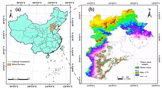
Figure 1.
(a) Location of the study area. (b) Winter wheat distribution (green) and winter wheat samples used to predict NDVI (red).
2.2. Data
2.2.1. Remote Sensing Data and Preprocessing
MOD09A1 surface reflectance product data were used in this study. These data provide bands 1–7 at a 500-meter resolution in an 8-day gridded level-3 product, and geometric, radiometric and atmospheric corrections were applied. The time series MODIS image collection was then used to calculate the NDVI using Equation (1):
where and are the surface reflectance values of the red band (0.62–0.67 μm) and the near-infrared band (0.84–0.87 μm) of the Modis sensor, respectively. Continuous long time series NDVI data were obtained from the Google Earth Engine (GEE) platform (https://earthengine.google.com, accessed on 4 May 2021), which allows parallelized processing of geospatial data on a global scale [36]. The time range of the data is from 1 January 2016 to 22 April 2020, with a spatial resolution of 500 meters and a temporal resolution of 8 days. A total of 107 images were collected. In Hebei province, winter wheat and corn are grown in a rotation, so the influence of corn data on the prediction of the winter wheat NDVI must be removed. Winter wheat is generally planted in October, returned to green jointing the following spring, and harvested in June. Therefore, in order to predict the NDVI of winter wheat, in this study, we chose 1 January to 30 June of the year after planting as the growth cycle of winter wheat for forecasting. The main phenological phases of winter wheat occur during this time period.
2.2.2. Winter Wheat Map
The map of winter wheat agriculture in 2018 was provided by Zhao et al. [37]. The spatial resolution of the map was 500 m and its overall accuracy was 94.74%. The total winter wheat planting area in the study region changed by less than 2% from 2015 to 2020 (http://www.stats.gov.cn, accessed on 10 May 2021). Therefore, the distribution of winter wheat fields was quite stable, and annual winter wheat maps were not required [38].
3. Methods
The method used in this paper is a combined DTW and LSTM method based on the MODIS NDVI time series data and the winter wheat map described above. Firstly, the winter wheat distribution and MODIS NDVI remote sensing data were combined to generate a winter wheat NDVI time series, and 500 NDVI time series were randomly selected for NDVI prediction. Secondly, the NDVI time series were decomposed into low-frequency time series and high-frequency time series by using FFT for waveform decomposition. Third, the low-frequency time series was predicted via DTW, and the high-frequency time series was predicted via LSTM. The DTW and LSTM prediction methods both used a rolling prediction method. A prediction value was predicted using the historical NDVI, and then this prediction value was treated as the historical NDVI value; the next value was predicted again, and after several iterations, multi-step prediction was performed. Finally, the results predicted by the two methods were synthesized to obtain the final prediction results and evaluate prediction accuracy (Figure 2).
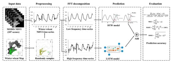
Figure 2.
Workflow of the proposed DTW–LSTM combination method.
3.1. FFT Decomposition
Using FFT, the signal can be transformed from the time domain to the frequency domain, allowing the spectrum structure and change law of the signal to be obtained [39,40,41]. FFT is often used for signal decomposition [33,34,35]. Loyarte et al. used the FFT to decompose the NDVI time series to obtain the average signal and sinusoidal components, which further leads to the average NDVI, amplitude and phase. Srivastava and Dikshit used FFT decomposition to obtain the dominant frequencies representing seasonality. Kocaaslan et al. used FFT for frequency analysis of drought indices. The process of signal decomposition using FFT is generally in three steps. Firstly, we transformed the original signal using the FFT algorithm and transformed the signal from the time domain to the frequency domain. Next, we filtered the signal using a high pass filter and a low pass filter. Finally, we transformed the filtered signal by inverse FFT (IFFT) to obtain the decomposed high-frequency and low-frequency signals.
3.2. DTW Model
Suppose that the time series with two lengths m and n are: P = (P1, P2, P3,…,Pm), Q = (Q1, Q2, Q3, …, Qn). First, the distance matrix of two-time series D (Equation (2)) is constructed. Secondly, matrix (Equation (3)) of the cumulative distance sequence is calculated. According to the cumulative distance sequence matrix, can be obtained.
where is the DTW distance between time series P and Q, and is the minimum cumulative distance from (1,1) to (m, n).
The schematic diagram of time series prediction using the DTW algorithm is shown in Figure 3, the time series is , where T represents the length of a complete winter wheat growth cycle, n represents the number of growth cycles, and is the value to be predicted. The specific steps to obtain are as follows:
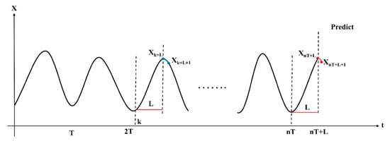
Figure 3.
Schematic diagram of time series prediction using the DTW algorithm.
- (1)
- Determine the two time -series A and B for which the DTW distance will be calculated.and . The length of the two time series is set to L.
- (2)
- Calculate the DTW distance between A and , denoted as . The specific method for DTW distance calculation is shown in Equations (2) and (3).
- (3)
- Find the time series . The DTW distance between and A has the minimum value.
- (4)
- The predicted value can be obtained by .
- (5)
- Bring as known data into the original winter wheat NDVI time series, and repeat steps (1) to (4).
Algorithm 1 can be used to express the entire process:
| Algorithm 1 Time series prediction algorithm based on the DTW algorithm |
| Input: is the historical winter wheat NDVI time series. T represents the length of a complete winter wheat growth cycle. n represents the number of growth cycles. L represents length of the time series of the last incomplete cycle. Output: predict length is the length of the forecast. In this study, predict length is set to 5. for i = 0: predict length -1 do for j = 0: nT– L do The method of calculating DTW distance is shown in Equations (2) and (3). end for K = minindex(C) end for return |
The DTW prediction model used the similarity in the growth patterns of winter wheat in different years to make predictions. Although the inter-annual NDVI curve of winter wheat is affected by meteorological factors (e.g., temperature, precipitation), and the waveform amplitude and phase will thus change, the overall similarity of the waveform is high, so the DTW algorithm can be used to find the NDVI curve that is most similar to the NDVI curve of the predicted year; this method is simple and easy to implement, and over-fitting is difficult. In this study, since the low-frequency time series after decomposition by FFT variation reflects the inter-annual and seasonal characteristics of winter wheat, the low-frequency time series was predicted using the DTW model. However, the short-term variation characteristics of the winter wheat NDVI reflected by the high-frequency time series after FFT decomposition have low waveform similarity within each winter wheat growth period, so this time series was not suitable for prediction by this model. The LSTM model was used for high-frequency time series prediction in the present study.
3.3. LSTM Model
The LSTM model was first reported by Hochreiter et al. in 1997 [42]. The efficient RNN structure of the LSTM model makes it well-suited for long-term dependent time series data [31]. RNNs are mainly used for nonlinear time-varying problems. The internal structure of a RNN makes it possible for data to advance and feedback backward. The nature of the feedback connection allows the algorithm to easily deal with the forward step. The residual value or weight value is updated, and this characteristic is well-suited for time series forecasting; it allows extraction of rules from the historical data of the time series to predict the future value of the time series. However, RNNs do not solve the issues of gradient disappearance and gradient explosion in network training.
The network structure of the general LSTM is shown in Figure 4, while a mathematical representation of a single LSTM network unit is provided in Equation (4).
where , , and represent the outputs of three sigmoid functions , which have values between 0 and 1. controls the flow of information from the old cell state , controls the flow of information from the cell activation . The hidden state is obtained from the output signal and the current cell state . , , , and are the weights applied to the concatenation of the new input and output from a previous cell. , , , and are the corresponding biases.
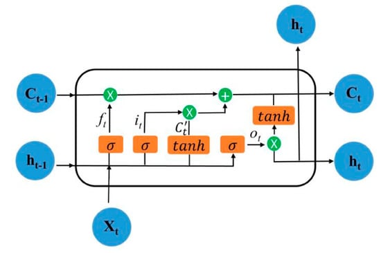
Figure 4.
Long short-term memory network structure.
The purpose of LSTM neural network design is to overcome the issues of gradient vanishing and gradient explosion, which are encountered when simple RNNs handle long-term dependent time series. The LSTM neural network model adds an input gate, an output gate and a forget gate [3,43]. The settings of relevant LSTM parameters are shown in Table 1.

Table 1.
Setting of LSTM parameters.
Time step is the sequence segment length, Rnn unit is the number of nodes in the fully connected layer, Batch size is the number of batches of sequence segments used for training. Input size is the dimension of the input data, Output size is the dimension of the output data, Learning rate is a hyper-parameter that determines the speed of training convergence, and Predict num is the length of the forecast data.
3.4. DTW–LSTM Combination Model
Based on the advantages of DTW and LSTM, we developed a DTW–LSTM combination model to predict the NDVI. Firstly, we decomposed the NDVI time series into a low-frequency signal and a high-frequency signal by FFT waveform decomposition. The low-frequency signal reflected the inter-annual NDVI variation, whereas the high-frequency signal reflected rapid NDVI changes caused by various factors. Secondly, we used DTW to predict the low-frequency signal and LSTM to predict the high-frequency signal. Finally, we combined the results of the DTW and LSTM predictions to obtain the final prediction.
3.5. Prediction Accuracy Evaluation
In this study, the Pearson correlation coefficient (r), mean absolute error (MAE), mean absolute percentage error (MAPE) and root mean square error (RMSE) were used to determine the predictive performance of the model. The r, MAE, and RMSE were defined as follows:
where represents the number of samples, is the observed NDVI value, is the predicted NDVI value, and is the average observed NDVI value. is the average predicted NDVI value.
4. Results
4.1. The Characteristics of Winter Wheat NDVI Time Series
The statistical characteristics of a winter wheat time series were analyzed (Figure 5). The winter wheat time series had a cyclical trend and short time variation (Figure 5a). The NDVI of winter wheat gradually changes every year from a small value to a large value, and then back to a small value, consistent with the inter-annual variation of the greenness of winter wheat. In January, the NDVI value is relatively small and fluctuates around 0.2. At this time, the wheat is in the overwintering period. In February and March, the NDVI gradually increases to approximately 0.3 to 0.4. When wheat enters the greening up stage in April and May, the NDVI increases rapidly and reaches its maximum value of approximately 0.6; this period corresponds with the jointing and heading stages of wheat. In June, the wheat slowly enters the mature period, when it gradually turns yellow, greenness decreases, and the NDVI gradually drops to a very low level. In addition to inter-annual and seasonal characteristics, the NDVI curve also has obvious short-term instantaneous changes. For example, in 2017, the NDVI decreased suddenly, and this change was likely caused by winter snow cover. As shown in Figure 5b, after a delay of order 30, most of the autocorrelation function values were outside the blue baseline of two times the standard deviation, and their correlation coefficients did not decay rapidly toward 0. This finding and the time series plot indicate a non-stationary time series. As shown in Figure 5c, the partial autocorrelation function (PACF) has similar characteristics to the autocorrelation function. The quantile–quantile (QQ) plot is a type of scatter plot in which the horizontal coordinate is the quantile of one sample and the vertical coordinate is the quantile of another sample. By a quantile, we mean the point below which a given fraction (or percent) of points lies. That is, the 0.2 (or 20%) quantile is the point at which 20% percent of the data fall below that value and 80% fall above that value. The scatter plot consisting of horizontal and vertical coordinates represents the quantile of the same cumulative probability. If the scatter plot is distributed around the line y = x, the two samples have the same distribution. In Figure 5d, we set the distribution of the horizontal coordinate sample to be normal. As shown in Figure 5d, the scatter plot does not tend to be distributed around the straight line, y = x, so this winter wheat time series does not conform to a normal distribution. A probability–probability (PP) plot is a scatter plot drawn from the cumulative probability of a variable corresponding to the cumulative probability of a particular theoretical distribution, and it is applied to determine whether a set of sample data fits a particular probability distribution. As shown in Figure 5e, the results of the PP plot are very similar to the QQ plot in Figure 5d; however, the PP plot uses the cumulative ratio of the distribution for the test, while the QQ plot uses the quartiles of the distribution. Since the scatter plot is not distributed on the straight line, y = x, this result is further evidence that the winter wheat time series sample data do not conform to a normal distribution.
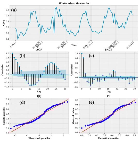
Figure 5.
Statistical characteristics of the winter wheat time series. (a) The original winter wheat time series. (b) Autocorrelation function (ACF). (c) Partial autocorrelation function (PACF). (d) Quantile–quantile plot (QQ). (e) Probability–probability plot (PP).
4.2. FFT Decomposition Results
Before NDVI prediction, it is necessary to perform FFT decomposition of the original NDVI time series curve to obtain low-frequency signals and high-frequency signals. Figure 6 shows the results of winter wheat NDVI time series curve decomposition using FFT. Figure 6a–c represent the original winter wheat NDVI time series and its amplitude–frequency characteristics and phase–frequency characteristics, respectively. Figure 6d–f represent the low-frequency time series and high-frequency time series after performing FFT decomposition and the corresponding amplitude–frequency characteristics and phase–frequency characteristics, respectively. As shown in Figure 6a, the winter wheat NDVI time series has seasonal slow changes and short-term transient changes from the time domain. As shown in Figure 6b, the winter wheat NDVI time series from the frequency domain has significant amplitude variation in the lower frequency part, which indicates that this winter wheat NDVI time series is mainly determined by this part, which corresponds to the seasonal slow variation only in the time domain. In addition, there are many components in the higher frequency part, but with small amplitude, and these components affect the specific values of the NDVI, which corresponds to short-term transient changes in the time domain. Figure 6c shows that the phase-frequency characteristic has no distinct features. Figure 6d shows the low-frequency and high-frequency time series after decomposition by FFT, which reveal that the NDVI values of the low-frequency time series are larger than those of the high-frequency time series. The waveform indicates that the low-frequency time series changes slowly, which corresponds exactly to the seasonal variation in the winter wheat time series, while the high-frequency time series corresponds exactly to the short-term transient variation. Figure 6e shows that from the frequency domain perspective, the spectrum of the low-frequency time series is mainly concentrated in the low-frequency part, and all of the high-frequency parts are 0. The spectrum of the high-frequency time series is mainly in the high-frequency part; there is also a part of the spectrum in the low-frequency part, but the amplitude of these components is small. Figure 6f shows the phase spectrum of the decomposed low-frequency and high-frequency time series, which reveal that the low-frequency time series has an approximately periodic pattern, while the high-frequency part has no obvious change characteristics.
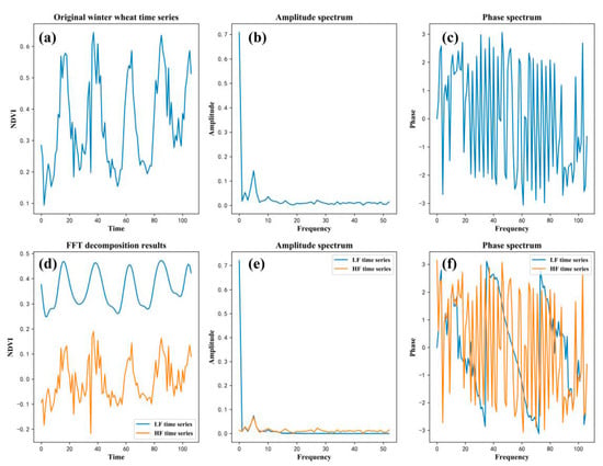
Figure 6.
FFT decomposition of winter wheat NDVI time series. (a) Original winter wheat time series. (b) Amplitude spectrum. (c) Phase spectrum. (d) FFT decomposition results. (e) Amplitude spectrum of low-frequency (LF) time series and high-frequency (HF) time series. (f) Phase spectrum of LF time series and HF time series.
4.3. Prediction Accuracy and Analysis
Figure 7 shows the scatter plot of the predicted NDVI and real NDVI values from 500 winter wheat time series, which were predicted using the DTW–LSTM method proposed in this paper. There are five prediction horizons in total. Because the time resolution is 8 days, the corresponding horizon is 8, 16, 24, 32 and 40 days ahead. Figure 7 shows that the predicted NDVI value is positively correlated with the observed NDVI value. On each prediction horizon, most points are below the 1:1 line, which indicates that the predicted NDVI value of most time series samples on each prediction horizon is less than the observed NDVI value. The linear correlation between the observed and predicted NDVI values weakens as the prediction horizon lengthens.
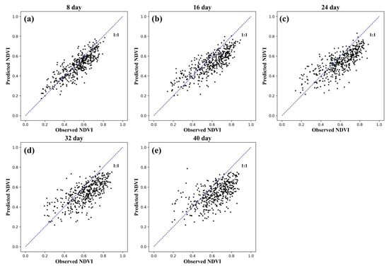
Figure 7.
Scatter plot of predicted and observed NDVI values using the DTW–LSTM method for different prediction horizons. (a) 8 days, (b) 16 days, (c) 24 days, (d) 32 days, (e) 40 days.
The r, MAE, MAPE and RMSE are shown in Table 2. The maximum value of r (0.825) was reached on the 8th day, when the MAE, MAPE, and RMSE reached minimum values of 0.065, 12.8% and 0.081, respectively. As the prediction horizon lengthens, r gradually decreases, while MAE, MAPE and RMSE gradually increase. The smallest r value (0.592) was measured on the 40th day, when the MAE, MAPE and RMSE reached 0.126, 20.6%, and 0.153, respectively. These findings show that NDVI prediction performance worsens due to accumulated error as the prediction scale increases.
Table 2.
r, MAE, MAPE and RMSE of predictions using the DTW–LSTM method for different prediction horizons.
To further analyze the NDVI prediction performance of the combined model, we compared the predicted NDVI value with the observed NDVI value for five prediction horizons (Figure 8). The green box plots show the observed NDVI values, and the red box plots show the predicted NDVI values. The change trend of the predicted five NDVI values is the same as the observed five NDVI values, and the predicted NDVI values are generally lower than the observed NDVI values. In addition, the variation ranges of the predicted NDVI values are smaller than those of the observed NDVI values. As the prediction horizon increases, the error between the predicted value and the observed value also increases (Figure 9). The prediction error between the predicted average NDVI value on 21 March and the observed average NDVI value is only 0.03. However, on 22 April, the prediction error reached 0.10.
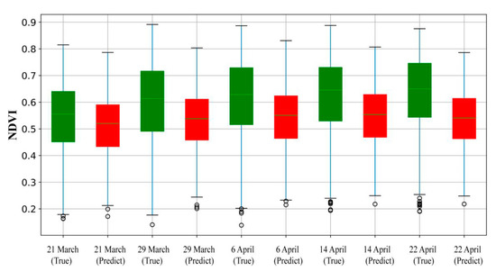
Figure 8.
Comparison of predicted NDVI values (red) and observed NDVI values (green).
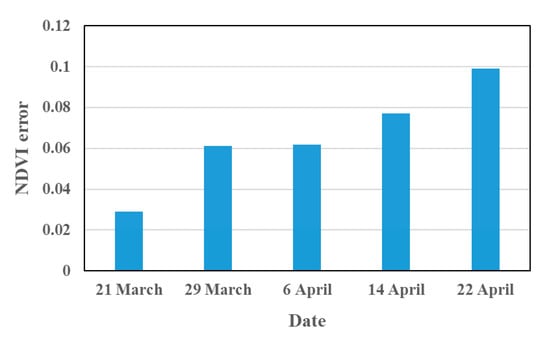
Figure 9.
The error between the predicted NDVI average value and the real NDVI average value.
5. Discussion
5.1. Comparison with the LSTM Method
Figure 10 shows a comparison of the combined DTW and LSTM method proposed in this article and the LSTM method. The performance of the combined method proposed in this study is better than that of the LSTM method for the five tested prediction horizons, and the MAE, MAPE, and RMSE of the combined method are all lower than those of the LSTM method. In terms of overall performance, the combined DTW and LSTM method proposed in this paper is better than the single LSTM method. Specifically, in terms of r, the LSTM method reached a value of only 0.745 on the 8th day, which is lower than that of the combined DTW–LSTM method (0.825) proposed in this paper. As the prediction horizon increases, r decreases gradually, and it drops to only 0.39 on the 40th day. Although the r value of the combined DTW–LSTM method also decreases gradually as the prediction horizon increases, the magnitude of the decrease is smaller than that of the LSTM method. The r value of the combined DTW–LSTM on the 40th day is 0.592, which is significantly larger than 0.39. In terms of MAE, although the MAE of both methods increases as the prediction scale increases, that of the combined DTW–LSTM method does not increase as much as that of the LSTM method, e.g., the MAE of the combined DTW–LSTM method is 0.126 on the 40th day, which is much smaller than that of the LSTM method (0.207). In terms of MAPE and RMSE, the trends are roughly the same as that of MAE.
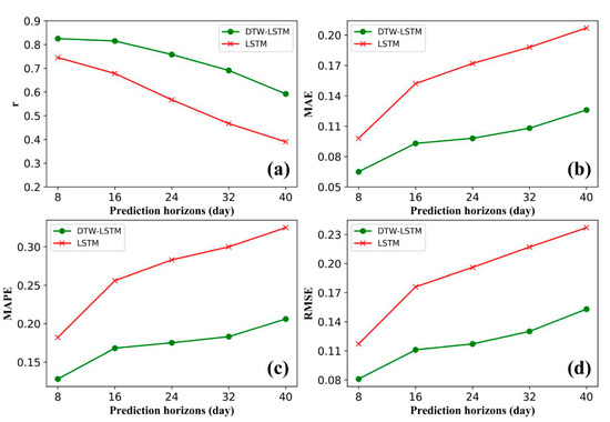
Figure 10.
Comparison of the predictions between DTW–LSTM model and LSTM. (a) r, (b) MAE, (c) MAPE, (d) RMSE.
Figure 11 shows the prediction performance of the DTW–LSTM method and the LSTM method in the context of the error distribution. The prediction errors of each method for different prediction horizons were considered, and the kernel density of the prediction error distribution was estimated using a Gaussian kernel [44]. As shown in Figure 11, the kernel density estimate (KDE) curves of the prediction errors for the DTW–LSTM model are denser than those of the LSTM method at the five prediction scales, with a mean value closer to 0. In addition, the kernel density curves of the prediction errors for the DTW–LSTM and LSTM methods become less dense as the prediction scale increases. On the 8th day, the prediction errors of the DTW–LSTM model are mainly distributed between −0.2 and 0.2, and those of the LSTM method are mainly distributed between −0.4 and 0.2. On the 40th day, the prediction errors of the DTW–LSTM model are mainly distributed between −0.4 and 0.4, and those of the LSTM method are mainly distributed between −0.6 and 0.4.
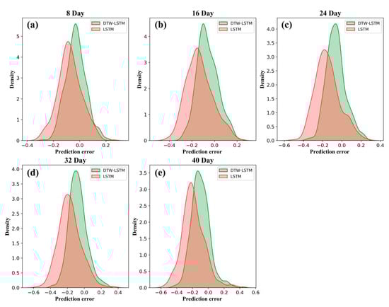
Figure 11.
Gaussian kernel density estimation of prediction errors using the DTW–LSTM and LSTM methods for different prediction horizons. (a) 8 days, (b) 16 days, (c) 24 days, (d) 32 days, (e) 40 days.
5.2. Limitations and Future Perspectives
This study has several limitations. First, a rolling prediction strategy was used to predict the decomposed high-frequency signal using LSTM, which allows multi-part prediction by considering the predicted NDVI value as the real NDVI value to participate in training and prediction to obtain the next predicted value. However, since there is an error between the predicted NDVI value and the observed NDVI value, the error accumulates as the number of prediction steps increases when multi-step prediction is performed, which gradually decreases the prediction accuracy. This error accumulation is confirmed by the prediction results in this paper. Second, NDVI prediction was performed directly based on historical NDVI time series. However, NDVI values are affected by meteorological factors such as temperature and precipitation, which can cause uncertainty regarding NDVI data and decrease the accuracy of NDVI prediction. Therefore, it is difficult to perform highly accurate predictions using NDVI time series only; accurate NDVI prediction requires a combination of different types of meteorological data, such as temperature and precipitation data.
Based on the limitations described above, we plan to focus on the following areas in our future research. In terms of methods, we can combine deep learning and crop models for NDVI prediction in order to improve prediction accuracy. In terms of data sources, predictions can be made by combining meteorological factors, such as temperature and precipitation, on the basis of NDVI data. In terms of prediction period, multi-scale predictions can be made to predict both short-term transient changes and long-term trend changes. In addition, based on the predicted NDVI, phenological phases and yield can be predicted more accurately.
6. Conclusions
In this paper, a combined DTW and LSTM method for predicting winter wheat NDVI was proposed, which utilizes the advantageous characteristics of both methods to achieve improved predictive performance in comparison with currently available models. This method uses the characteristics of inter-annual and short-term changes in the winter wheat NDVI. First, FFT is used to decompose the winter wheat NDVI sequence into two parts. One part reflects stable inter-annual and seasonal changes and uses the DTW algorithm for prediction, while the other part reflects random short-term NDVI changes and uses LSTM for prediction. The prediction results obtained with the combined DTW–LSTM model show that the prediction performance of the combined model is high when the prediction time is short. The combined DTW–LSTM method proposed in this report can also be applied to predict the NDVI of other crops.
Author Contributions
Conceptualization, F.Z. and G.Y.; data curation, F.Z., Y.Z., and S.H.; methodology, G.Y. and F.Z.; formal analysis, F.Z., Y.M. and X.B.; writing—original draft preparation, F.Z.; writing—review and editing, G.Y. and H.Y. All authors have read and agreed to the published version of the manuscript.
Funding
This research was funded by National Natural Science Foundation of China (No. 42171303), the Key-Area Research and Development Program of Guangdong Province (Nos. 2019B020214002 and 2019B020216001), the Beijing Million Talent Project (No. 2019A10), and the National Key Research and Development Program of China (No. 2017YFE0122500).
Institutional Review Board Statement
Not applicable.
Informed Consent Statement
Not applicable.
Data Availability Statement
The remote sensing data were obtained from the Google Earth Engine (GEE) platform (https://earthengine.google.com, accessed on 4 May 2021).
Acknowledgments
We would like to thank our collaborators from the Key Laboratory of Quantitative Remote Sensing in Agriculture of Ministry of Agriculture and Rural Affairs, National Engineering Research Center for Information Technology in Agriculture, and Anhui University. We also thank the anonymous reviewers and the academic editor for their valuable comments and recommendations.
Conflicts of Interest
The authors declare no conflict of interest.
References
- Hatfield, J.L.; Gitelson, A.A.; Schepers, J.S.; Walthall, C.L. Application of spectral remote sensing for agronomic decisions. Agron. J. 2008, 100, S117–S131. [Google Scholar] [CrossRef]
- Berger, A.; Ettlin, G.; Quincke, C.; Rodriguez-Bocca, P. Predicting the Normalized Difference Vegetation Index (NDVI) by training a crop growth model with historical data. Comput. Electron. Agric. 2019, 161, 305–311. [Google Scholar] [CrossRef]
- Ahmad, R.; Yang, B.; Ettlin, G.; Berger, A.; Rodriguez-Bocca, P. A machine-learning based ConvLSTM architecture for NDVI forecasting. Int. Trans. Oper. Res. 2020, 12887. [Google Scholar] [CrossRef]
- Huang, J.; Han, D.W. Meta-analysis of influential factors on crop yield estimation by remote sensing. Int. J. Remote Sens. 2014, 35, 2267–2295. [Google Scholar] [CrossRef]
- Xue, J.R.; Su, B.F. Significant Remote Sensing Vegetation Indices: A Review of Developments and Applications. J. Sens. 2017, 2017, 1353691. [Google Scholar] [CrossRef]
- Yan, L.; Roy, D.P. Automated crop field extraction from multi-temporal Web Enabled Landsat Data. Remote Sens. Environ. 2014, 144, 42–64. [Google Scholar] [CrossRef]
- Estel, S.; Kuemmerle, T.; Alcantara, C.; Levers, C.; Prishchepov, A.; Hostert, P. Mapping farmland abandonment and recultivation across Europe using MODIS NDVI time series. Remote Sens. Environ. 2015, 163, 312–325. [Google Scholar] [CrossRef]
- Fernandes, J.L.; Ebecken, N.F.F.; Esquerdo, J.C.D. Sugarcane yield prediction in Brazil using NDVI time series and neural networks ensemble. Int. J. Remote Sens. 2017, 38, 4631–4644. [Google Scholar] [CrossRef]
- Cui, C.L.; Zhang, W.; Hong, Z.M.; Meng, L.K. Forecasting NDVI in multiple complex areas using neural network techniques combined feature engineering. Int. J. Digit. Earth 2020, 13, 1733–1749. [Google Scholar] [CrossRef]
- Ivits, E.; Cherlet, M.; Sommer, S.; Mehl, W. Addressing the complexity in non-linear evolution of vegetation phenological change with time-series of remote sensing images. Ecol. Indic. 2013, 26, 49–60. [Google Scholar] [CrossRef]
- Monday, M. Forecasting the Interannual Trends in Terrestrial Vegetation Dynamics Using Time Series Modelling Techniques. In ForestSAT Symposium Heriot Watt University; Heriot Watt University: Edinburgh, UK, 2002. [Google Scholar]
- Li, B.; Tao, S.; Dawson, R.W. Relations between AVHRR NDVI and ecoclimatic parameters in China. Int. J. Remote Sens. 2002, 23, 989–999. [Google Scholar] [CrossRef]
- Ji, L.; Peters, A.J. A spatial regression procedure for evaluating the relationship between AVHRR-NDVI and climate in the northern Great Plains. Int. J. Remote Sens. 2004, 25, 297–311. [Google Scholar] [CrossRef]
- Propastin, P.A.; Kappas, M. Reducing uncertainty in modeling the NDVI-precipitation relationship: A comparative study using global and local regression techniques. Gisci. Remote Sens. 2008, 45, 47–67. [Google Scholar] [CrossRef]
- Fernandez-Manso, A.; Quintano, C.; Fernandez-Manso, O. Forecast of NDVI in coniferous areas using temporal ARIMA analysis and climatic data at a regional scale. Int. J. Remote Sens. 2011, 32, 1595–1617. [Google Scholar] [CrossRef]
- Yue, L.W.; Shen, H.F.; Zhang, L.P.; Zheng, X.W.; Zhang, F.; Yuan, Q.Q. High-quality seamless DEM generation blending SRTM-1, ASTER GDEM v2 and ICESat/GLAS observations. ISPRS J. Photogramm. 2017, 123, 20–34. [Google Scholar] [CrossRef]
- Zang, L.; Mao, F.Y.; Guo, J.P.; Wang, W.; Pan, Z.X.; Shen, H.F.; Zhu, B.; Wang, Z.M. Estimation of spatiotemporal PM1.0 distributions in China by combining PM2.5 observations with satellite aerosol optical depth. Sci. Total Environ. 2019, 658, 1256–1264. [Google Scholar] [CrossRef]
- Atkinson, P.M.; Tatnall, A.R.L. Introduction Neural networks in remote sensing. Int. J. Remote Sens. 1997, 18, 699–709. [Google Scholar] [CrossRef]
- Mas, J.F.; Flores, J.J. The application of artificial neural networks to the analysis of remotely sensed data. Int. J. Remote Sens. 2008, 29, 617–663. [Google Scholar] [CrossRef]
- Kang, L.; Di, L.; Deng, M.; Yu, E.; Xu, Y. Forecasting vegetation index based on vegetation-meteorological factor interactions with artificial neural network. In Proceedings of the 2016 5th International Conference on Agro-Geoinformatics (Agro-Geoinformatics), Tianjin, China, 18–20 July 2016. [Google Scholar]
- Nay, J.; Burchfield, E.; Gilligan, J. A machine-learning approach to forecasting remotely sensed vegetation health. Int. J. Remote Sens. 2018, 39, 1800–1816. [Google Scholar] [CrossRef]
- Stepchenko, A.; Chizhov, J. NDVI Short-Term Forecasting Using Recurrent Neural Networks. Environ. Technol. Resour. Proc. Int. Sci. Pract. Conf. 2015, 3, 180. [Google Scholar] [CrossRef]
- Reddy, D.S.; Prasad, P.R.C. Prediction of vegetation dynamics using NDVI time series data and LSTM. Modeling Earth Syst. 2018, 4, 409–419. [Google Scholar] [CrossRef]
- Wu, T.S.; Fu, H.P.; Feng, F.; Bai, H.M. A new approach to predict normalized difference vegetation index using time-delay neural network in the arid and semi-arid grassland. Int. J. Remote Sens. 2019, 40, 9050–9063. [Google Scholar] [CrossRef]
- Sakoe, H.; Chiba, S. Dynamic Programming Algorithm Optimization for Spoken Word Recognition. IEEE Trans. Acoust. Speech Signal Process. 1978, 26, 43–49. [Google Scholar] [CrossRef]
- Petitjean, F.; Inglada, J.; Gancarski, P. Satellite Image Time Series Analysis Under Time Warping. IEEE Trans. Geosci. Remote 2012, 50, 3081–3095. [Google Scholar] [CrossRef]
- Petitjean, F.; Weber, J. Efficient Satellite Image Time Series Analysis Under Time Warping. IEEE Geosci. Remote Sens. 2014, 11, 1143–1147. [Google Scholar] [CrossRef]
- Costa, W.S.; Fonseca, L.M.G.; Korting, T.S.; Bendini, H.D.; de Souza, R.C.M. Spatio-Temporal Segmentation Applied to Optical Remote Sensing Image Time Series. IEEE Geosci. Remote Sens. 2018, 15, 1299–1303. [Google Scholar] [CrossRef]
- Xue, Z.H.; Du, P.J.; Feng, L. Phenology-Driven Land Cover Classification and Trend Analysis Based on Long-term Remote Sensing Image Series. IEEE J. Sel. Top. Appl. Earth Obs. Remote Sens. 2014, 7, 1142–1156. [Google Scholar] [CrossRef]
- Maus, V.; Camara, G.; Cartaxo, R.; Sanchez, A.; Ramos, F.M.; de Queiroz, G.R. A Time-Weighted Dynamic Time Warping Method for Land-Use and Land-Cover Mapping. IEEE J. Sel. Top. Appl. Earth Obs. Remote Sens. 2016, 9, 3729–3739. [Google Scholar] [CrossRef]
- Xiao, C.J.; Chen, N.C.; Hu, C.L.; Wang, K.; Gong, J.Y.; Chen, Z.Q. Short and mid-term sea surface temperature prediction using time-series satellite data and LSTM-AdaBoost combination approach. Remote Sens. Environ. 2019, 233, 111358. [Google Scholar] [CrossRef]
- Cooley, J.W.; Tukey, J.W. An Algorithm for the Machine Calculation of Complex Fourier Series. Math. Comput. 1965, 19, 297–301. [Google Scholar] [CrossRef]
- Loyarte, M.M.G.; Menenti, M.; Diblasi, A.M. Modelling bioclimate by means of Fourier analysis of NOAA-AVHRR NDVI time series in Western Argentina. Int. J. Climatol. 2008, 28, 1175–1188. [Google Scholar] [CrossRef]
- Srivastava, S.; Dikshit, O. Seasonal and trend analysis of TWS for the Indo-Gangetic plain using GRACE data. Geocarto Int. 2020, 35, 1343–1359. [Google Scholar] [CrossRef]
- Kocaaslan, S.; Musaoglu, N.; Karamzadeh, S. Evaluating Drought Events by Time-Frequency Analysis: A Case Study in Aegean Region of Turkey. IEEE Access 2021, 9, 125032–125041. [Google Scholar] [CrossRef]
- Gorelick, N.; Hancher, M.; Dixon, M.; Ilyushchenko, S.; Thau, D.; Moore, R. Google Earth Engine: Planetary-scale geospatial analysis for everyone. Remote Sens. Environ. 2017, 202, 18–27. [Google Scholar] [CrossRef]
- Zhao, F.; Yang, G.J.; Yang, X.D.; Cen, H.Y.; Zhu, Y.H.; Han, S.Y.; Yang, H.; He, Y.; Zhao, C.J. Determination of Key Phenological Phases of Winter Wheat Based on the Time-Weighted Dynamic Time Warping Algorithm and MODIS Time-Series Data. Remote Sens. 2021, 13, 1836. [Google Scholar] [CrossRef]
- Gan, L.Q.; Cao, X.; Chen, X.H.; Dong, Q.; Cui, X.H.; Chen, J. Comparison of MODIS-based vegetation indices and methods for winter wheat green-up date detection in Huanghuai region of China. Agric. For. Meteorol. 2020, 288, 108019. [Google Scholar] [CrossRef]
- Marquezino, F.L.; Portugal, R.; Sasse, F.D. Obtaining the Quantum Fourier Transform from the classical FFT with QR decomposition. J. Comput. Appl. Math. 2010, 235, 74–81. [Google Scholar] [CrossRef]
- Zhang, Y.L.; Gao, Y.; Jiang, P.S.; Xu, H.Y. Study of Polyphase Decomposition Zoom-FFT Algorithm in Non-Invasive Motor Monitoring System. In Advanced Materials Research; Trans Tech Publications Ltd.: Freienbach, Switzerland, 2011; pp. 1452–1457. [Google Scholar]
- Ahamed, S.F.; Rao, G.S.; Ganesh, L. Fast Acquisition of GPS Signal Using FFT Decomposition. Procedia Comput. Sci. 2016, 87, 190–197. [Google Scholar] [CrossRef]
- Hochreiter, S.; Schmidhuber, J. Long Short-Term Memory. Neural Comput. 1997, 9, 1735–1780. [Google Scholar] [CrossRef]
- Wang, J.Y.; Li, J.Z.; Wang, X.X.; Wang, J.; Huang, M. Air quality prediction using CT-LSTM. Neural Comput. Appl. 2021, 33, 4779–4792. [Google Scholar] [CrossRef]
- Dehnad, K. Density Estimation for Statistics and Data Analysis. Technometrics 2012, 29, 495. [Google Scholar] [CrossRef]


Publisher’s Note: MDPI stays neutral with regard to jurisdictional claims in published maps and institutional affiliations. |
© 2021 by the authors. Licensee MDPI, Basel, Switzerland. This article is an open access article distributed under the terms and conditions of the Creative Commons Attribution (CC BY) license (https://creativecommons.org/licenses/by/4.0/).