High-Resolution Direct Push Sensing in Wetland Geoarchaeology—First Traces of Off-Site Construction Activities at the Fossa Carolina

Abstract

Wetland environments, with their excellent conservation conditions, provide geoarchaeological archives of past human activities. However, the subsurface soil is difficult to access due to high groundwater tables, unstable sediments, and the high cost of excavation. In this study, we present a ground-based non- and minimal-invasive prospection concept adapted to the conditions of wetlands. We investigated the Fossa Carolina in South Germany, a canal that was intended in 792/793 AD by Charlemagne to bridge the Central European Watershed. Although the resulting Carolingian banks and the fairway with wooden revetments are very imposing, archaeological traces of off-site construction activities have not been identified hitherto. Based on a geophysically surveyed intensive linear magnetic anomaly parallel to the Carolingian canal, we aimed to prove potential off-site traces of Carolingian construction activities. In this context, we built up a high-resolution cross-section using highly depth-accurate direct push sensing and ground-truthing. Our results showed the exact geometry of the canal and the former banks. Thus, the magnetic mass anomaly could be clearly located between the buried organic-rich topsoil and the Carolingian banks. The thermoluminescence dating showed that the position of the magnetic mass anomaly reflected Carolingian activities during the construction phases, specifically due to heat exposure. Moreover, we found hints of the groundwater supply to the 5-metre wide navigable fairway.

1. Introduction

1.1. Challenging Issues in Geoarchaeological Wetland Exploration

Wetlands provide important geoarchaeological archives about past landscape development, e.g., [1,2,3] as well as buried infrastructure and settlements, e.g., [4,5,6]. However, unfavourable properties like unstable sediments and a high groundwater table lead to high costs for direct access by excavations [7,8,9]. The post-excavation conservation of archaeological materials is expensive and complicated as well [10,11]. Thus, there is a demand for remote, non-invasive, and minimal-invasive exploration approaches for cross-scale, multi-method, and systematic surveys in wetland geoarchaeology in order to investigate, but also to monitor, vulnerable archaeological features, e.g., pile dwellings.

In addition, non-invasive geophysical surveys can be conducted from large to small spatial scales [9] in a cost-saving way in a wide range of combinations. They offer different sensitivities depending on physical material characteristics, e.g., suspicious values of the magnetic field strength of fire-affected sediments or striking values of electrical conductivity of saturated ditch fillings, e.g., [12,13]. However, they need sufficient contrast of the material characteristics in the subsurface soil [14,15] and ideally, ground truth data for reliable interpretations [16,17]. In general, for effective conduction and credible results of non- and minimal-invasive exploration methods, a well thought-out field strategy with the on-site decision [18] as well as a combination of carefully selected parameters with suitable sensitivities for the targeted features are necessary [14,19,20].

In terms of ground-truthing, minimally invasive vibracoring provides important point-by-point insight into the sediments and sampling opportunities, e.g., [21,22], but can record depths inaccurately, especially in wetlands caused by high compaction rates of the sediments [23]. Another method that has been applied recently as an alternative to ground truth [17,24] and for geoarchaeological exploration per se on decametre to sub-metre scale [16,25,26] is minimal-invasive and depth-accurate direct push sensing [27,28]. The colour logging tool (e.g., for peat detection [26,29]) and electrical conductivity logging (e.g., for sediment unit surveys [24,25]) have proven successful in geoarchaeological studies.

1.2. The Fossa Carolina—Previous Geoarchaeological Findings

The Fossa Carolina is an Early Medieval canal in southern Germany located in the foothills of the Southern Franconian Alb (Figure 1). The canal was designed in 792 AD and built in 792/793 AD by Charlemagne, linking the Rhine and Danube river systems and thus bridging the Central European Watershed, which is confirmed by dendrochronological dating [4,30] and written sources [30,31,32]. Small altitude differences (approximately 6 m) and the short distance between the Altmühl and Swabian Rezat rivers (approximately 2 km as the crow flies) provided favourable conditions for this project [23,33,34].

The canal is approximately 3 km in length and has a conspicuous s shape (Figure 1c) in order to minimise the work needed to complete the respective section [35]. According to dendroarchaeological findings, it is assumed that the work progressed from north to south towards the summit [36]. However, the southernmost part of the canal was never finished, as no archaeological remains were detected in the Altmühl floodplain [37]. Written sources explain this abandonment as being due to unstable trench edges and strong rainfalls [31]. Subsequently, the trenched areas were used as ponds to some extent until they were completely silted up [23,38].

The construction of the summit canal was designed as a stepped chain of ponds with approximately 2.5–5 m fairway width [4,29,30,39] and a northward shifted summit [36,39]. Large oak timbers were used for the stabilisation of the canal edges. The canal can be divided into different sections (Figure 1c). The central section and the west–east section are still marked by impressive banks from Carolingian excavation works. After a bend to the north, the banks become more and more shallow in the northern section, and the course of the canal is hardly to not at all visible in the northernmost north-eastern section [39,40].

Figure 1. Overview of the Fossa Carolina: (a) Supra-regional perspective. (b) Location of the Central European Watershed separating the Rhine-Main and the Danube river systems. (c) The different canal sections (orange font) with the Swabian Rezat and Altmühl Rivers. (Database: European Environment Agency [41], OSM—Open Street Map, Zielhofer et al. [39], LiDAR data are provided by the Bavarian Land Surveying Office).

Figure 1. Overview of the Fossa Carolina: (a) Supra-regional perspective. (b) Location of the Central European Watershed separating the Rhine-Main and the Danube river systems. (c) The different canal sections (orange font) with the Swabian Rezat and Altmühl Rivers. (Database: European Environment Agency [41], OSM—Open Street Map, Zielhofer et al. [39], LiDAR data are provided by the Bavarian Land Surveying Office).

1.3. Linear Magnetic Anomaly at the Fossa Carolina

A large-scale superconducting quantum interference device (SQUID) magnetic survey [42] revealed a conspicuous anomaly parallel to the canal course in the northern and southernmost north-eastern section (Figure 2). Especially noticeable are the straight course and the interruptions (Figure 2e). In the grid view (range ± 10 nT/m), the anomaly is usually approximately between 7 and 8 m wide. The segment lengths vary between approximately 30 and 80 m. In situ volume magnetic susceptibility (κ) measurements at the anomaly’s position (core QP2 position in Figure 2b, [43]) revealed the highest values of approx. 45,000 × 10⁻⁶ SI at depths between 135 and 155 cm, where the magnetic mass anomaly is characterised by black, reddish-brown, and red colours. Further rock-magnetic laboratory analysis indicated a titanomagnetite/magnetite layer, which required heating over 700 °C [43]. However, to date, there is no reliable stratigraphic positioning of the anomaly, no age control, and therefore no clear knowledge about its possible origin.

1.4. Aims of this Study

In this study, (i) we aimed to apply an advanced minimal-invasive, multi-method approach at the buried wetland site to explore the intensive magnetic anomaly. We combine direct push colour and electrical conductivity logging for a full 2D cross-section beyond the vertical and lateral borders of the Fossa Carolina and link the data with vibracoring ground truth data and subsequent laboratory analysis.

Then, we aimed to (ii) reconstruct the chronostratigraphy of the Carolingian canal fills and adjacent banks in order to determine the exact stratigraphic position of the magnetic mass anomaly outside the canal course. Doing so will provide chronological control for what is likely to be the first traces of Carolingian off-site construction activities. Moreover, we aimed to collect evidence concerning navigability and the potential water supply.

2. Geographical Setting of the Fossa Carolina

The Fossa Carolina is located in the foothills of the Franconian Jura escarpment (Figure 3). The valley floors are characterised by clayey to sandy glacio-fluvial sediments from the Last Glacial. Holocene fen deposits (Rezat Fen), as well as Holocene flood deposits in the Altmühl and Rezat floodplains, have built up the present surface [33,44,45].

The geological composition and topography determine the hydrological setting. In the valley, Middle Jurassic and Miocene clayey sequences sealed the valley bottom. At the foothill positions, Middle and Upper Jurassic clayey sequences [46] correspond with spring horizons, e.g., the Swabian Rezat spring [33,44,45]. In the northern section of the canal, the continuously increasing discharge of the Swabian Rezat river points to a substantial groundwater supply because tributaries are absent in this zone [47]. These conditions lead to a high groundwater table that is indicated by the presence of the Rezat Fen and buried organic-rich topsoil that is widespread [8,16,33].

3. Methods

3.1. SQUID Magnetic Prospection and Depth Calculation of Intensive Magnetic Anomalies

For the large-scale magnetic prospection (Figure 4), a motorised SQUID measuring instrument [48,49] was used. The high-resolution device recorded magnetic subsurface data with a configuration of 18 SQUID gradiometers and magnetometers. The corresponding position was localised synchronously by a differential GPS. Precisely georeferenced magnetograms of the entire canal area were created [42,50,51]. The recorded linear anomalies could not always be delineated sharply, for a variety of reasons, such as limited measurement possibilities (Figure 2e, segment 4) or a diffuse signal (Figure 2, segments 1 and 5). Segment 2 (Figure 2e), the segment that was investigated in our study in detail, is clearly recognisable. The subsurface distribution of the magnetic sources could be determined by the maxima of the magnetic information [52,53]. In this study, the un-gridded magnetic data of several SQUID sensors were used to calculate the depth of the magnetic sources from which the intense magnetic deviation originate. Calculation basics are the anomaly maxima and minima recorded by pairs of SQUID sensors [54] and a 1/r³ amplitude dependence from the source-sensor distance r. After the evaluation of the SQUID magnetic data, we performed high-resolution direct push sensing and laboratory analysis from depth-corrected vibracoring samples. For age control, we used both thermoluminescence and radiocarbon dating (Figure 4).

3.2. Direct Push Sensing

Direct push techniques provide a set of tools for minimal-invasive, depth-accurate in situ measurements by pushing steel rods equipped with different probes into the unconsolidated underground [27,55]. We used 38-millimetre steel rods at the colour logging tool (CLT) and the electrical conductivity probe (EC) that were driven by a Geoprobe 6610 DT caterpillar (Figure 5). Based on on-site decisions, our sampling points were placed in distances of 0.25 to 2 m from each other along the cross-section. The depths were precisely logged by a potentiometer. For exact localisation, we defined each position using a Topcon HiPer II DGPS with an accuracy of 10 mm horizontally and 15 mm vertically.

3.2.1. Colour Logging Tool (CLT)

We used colour measurements to differentiate sediments and analyse archaeological structures [26,29,56]. The Soil Colour Optical Screening Tool (SCOST™; Dakota Technologies, Fargo, ND, USA) recorded the colours in a range of 350–1000 nm and provided numerical colour values (RGB, XYZ, Munsell) in the visible range. A control unit sent white light via a fibre optic cable to the sapphire window in the probe, and then a detector measured the reflections over an adjusted time interval of approximately 300 ms. We used a propulsion of approximately 2 cm/s. A Spectralon and standardised white and black colours were used to calibrate the system before and after each measurement. OST Software (Dakota Technologies) recorded the colour values and generated a. jpg raster file from the RGB colour values. For post-processing, we calculated additional values of the CIE 1976 (L*a*b*) [57] colour space and applied the Wavelet filter to the data (Daubechies, Daublet 4) to smooth outliers [26,58].

We recorded 82 direct push colour logs with 0.25 to 0.5 m spacing. During the measurement and post-processing, we observed a variety of brightnesses in the central part of the cross-section (approx. between AN_CLT_74 to 43, from the surface to a depth of approx. 415.5 m a.s.l.), which probably reflected the wetness of the sediments. In general, the adhesion of sediment to the sapphire window can be excluded because of the high pressure exerted on the probe.

In our study, we displayed the .jpg raster images of each probe and adapted their width for a merged visualisation in the figure.

3.2.2. Electrical Conductivity Logging (EC)

The EC probe (SC-500; Keijr Engineering Inc., Geoprobe Systems, Salina, KS, USA) was used for the differentiation of sediment units. The probe is equipped with four electrodes in a Wenner array with a vertical alignment and a fixed distance of 2 cm. This enabled the analysis of layers with thicknesses ranging from 5 to 10 cm [59,60,61]. The probe measured the specific electrical resistivity, which is inversely expressed as the specific electrical conductivity in mS/m in fixed 1.5-centimetre steps [62,63].

The values represent a sum parameter of the sediment properties of grain size, fluid saturation, chemical properties, and salinity of the pore fluid [63,64]. In saturated sediments, relatively high values usually indicate fine-grained sediments, such as clay, and lower values indicate coarser-grained sediments, such as silt, sand, and gravel [62,63].

We added spacing between the individual electrical conductivity logs from 0.5 to 3 m.

3.3. Vibra-Coring

We used vibracoring for the ground-truthing and sediment sample recovery. The open cores (60 mm diameter, 1 m length) were driven by an Atlas Copco Cobra Pro motorised hammer and localised with the Topcon HiPer II DGPS. In the field, we documented sediment properties, soil horizons, and reductive-oxidative properties using the KA5 soil mapping guide [65] and Munsell colours [66]. We sampled sediment sequences with an eye to stratigraphical changes as well as in equidistant 5-centimetre steps and corrected the sample depths by matching core sequences with depth-accurate direct push RGB colour logs (Figure S1).

3.4. Laboratory Analysis

3.4.1. Grain Size Analysis

We used grain size distributions to identify sedimentological units and to interpret the related depositional processes. To remove organic components from the sample, we added hydrogen peroxide (H₂O₂, 50 mL, 35%) to 10 g of air-dried fine sediment (<2 mm). To dissolve sediment aggregates, we added sodium pyrophosphate (Na₄P₂O₇, 10 mL, 0.4 N) and treated the sample in an ultrasonic bath (45 min). The sand fraction was analysed by sieve analysis and the clay silt fraction by X-ray granulometry (XRG, Micromeritics Sedigraph III 5120). The grain size classes followed the KA5 soil mapping guide [65] in µm: coarse sand (cSa)—630 to < 2000, medium sand (mSa)—200 to 630, and fine sand (fSa)—63 to 200; coarse silt (cSi)—20 to 63, medium silt (mSi)—6.3 to 20, and fine silt (fSi)—2 to 6.3; and coarse clay (cCl)—0.6 to 2, medium clay (mCl)—0.2 to 0.63, and fine clay (fCl)—<0.2.

3.4.2. Geochemical and Rock Magnetic Sediment Analysis

We used elemental analysis by the vario EL cube (Elementar) to analyse the total content of sulphur, carbon, and nitrogen (CNS) to specify and divide the sediment stratigraphy. Furthermore, we used a Scheibler calcimeter (Eijkelkamp) to quantify inorganic carbon content. To calculate the organic carbon, we subtracted the inorganic carbon from the total carbon. We used laboratory measurements of volume-specific low-frequency magnetic susceptibility (κ, 0.465 kHz, 10⁻⁶ SI) to detect magnetic anomalies within the recovered cores. Then, we filled plastic cubes with the sediment and used a Bartington MS3 equipped with an MS2B dual-frequency sensor [67,68].

3.5. Age Control Measurements

3.5.1. Thermoluminescence (TL) Dating

Two samples were taken from the magnetic mass anomaly for TL dating because this is the most suitable luminescence method for heated material [69,70,71].

The samples were taken from an opaque core liner (core BK5) at depths of 135–140 cm (KG-TL1) and 150–155 cm (KG-TL2) and were subsequently prepared under subdued red light in the luminescence preparation room of the Institute of Geography at Leipzig University. Sample preparation included sieving with meshes with widths of 90 and 200 µm, treatments with 10% and 30% HCl for calcium carbonate destruction, and with 10% and 37% H₂O₂ over 14 days to destroy organic matter. Subsequently, the fine grain fraction (4–11 µm) was separated according to Stoke’s Law in Atterberg settling tubes.

In tandem with the luminescence samples, dose rate samples were taken from the core. The sample material from KG-TL1 was taken from its surroundings. Given that sample KG-TL2 was located near a stratigraphical border, one sample was taken from the light-coloured material above (156–140 cm; DL-1) and another from the dark-coloured material below (170–158 cm; DL-2). Both equivalent dose (De) and dose rate determinations were carried out in the luminescence laboratory of the Curt-Engelhorn-Centre of Archaeometry (Mannheim, Germany).

The De was measured with blue thermoluminescence (multiple aliquots according to Aitken [72]) using a Risø TL-DA-20 device equipped with a combination of BG3 and BG39 (both 3-millimetre thick) filters and a ⁹⁰Sr/⁹⁰Y β-source (0.079 Gy/s). The a value was determined with a 241 Am α-source (0.116 Gy/s).

The sediment dose rates (contents of the radioactive elements U, Th, and K) were measured with low-level γ–spectrometry using a Canberra GCW4023 high-purity Germanium well detector. The water content of the samples was determined gravimetrically by weighing the samples before and after drying at 105 °C for 24 h. The cosmic dose rate was calculated according to Prescott and Hutton [73], assuming a density of the overlying sediments of 1.6 g/cm³.

Possible anomalous fading of the samples was checked by measuring five irradiated and five not irradiated aliquots of every sample and comparing those results with identical measurements of the same number of aliquots after a storage time of approximately 6 weeks.

3.5.2. Radiocarbon Dating

Seeds, charcoal, wood fragments, and organic soil bulk samples were radiocarbon dated. The samples with the MAMS laboratory code were analysed at the Curt-Engelhorn-Centre of Archaeometry (Mannheim, Germany) with an accelerator mass spectrometry (AMS) type MICADAS [74]. The sample with the KIA laboratory code was analysed at the Leibniz Laboratory for Radiometric Dating and Stable Isotope Research at Kiel University using the type HVE 3MV Tandetron 4130 accelerator mass spectrometer (AMS) [75]. We calibrated all samples consistently with the INTCAL 13 dataset [76].

3.5.3. Age Control by Archaeological Findings

An adjacent archaeological excavation in 2013 (for location, see Figure 2) provided a high-resolution stratigraphy and age control [4] by archaeological finds like ceramics and horseshoe and the dendrochronological dating of oak timber, as well as by radiocarbon dating of short-lived botanical remains. We used these chronostratigraphic findings to refine our understanding of the canal-fill stratigraphy within our recently conducted direct push cross-section.

4. Results and Interpretation

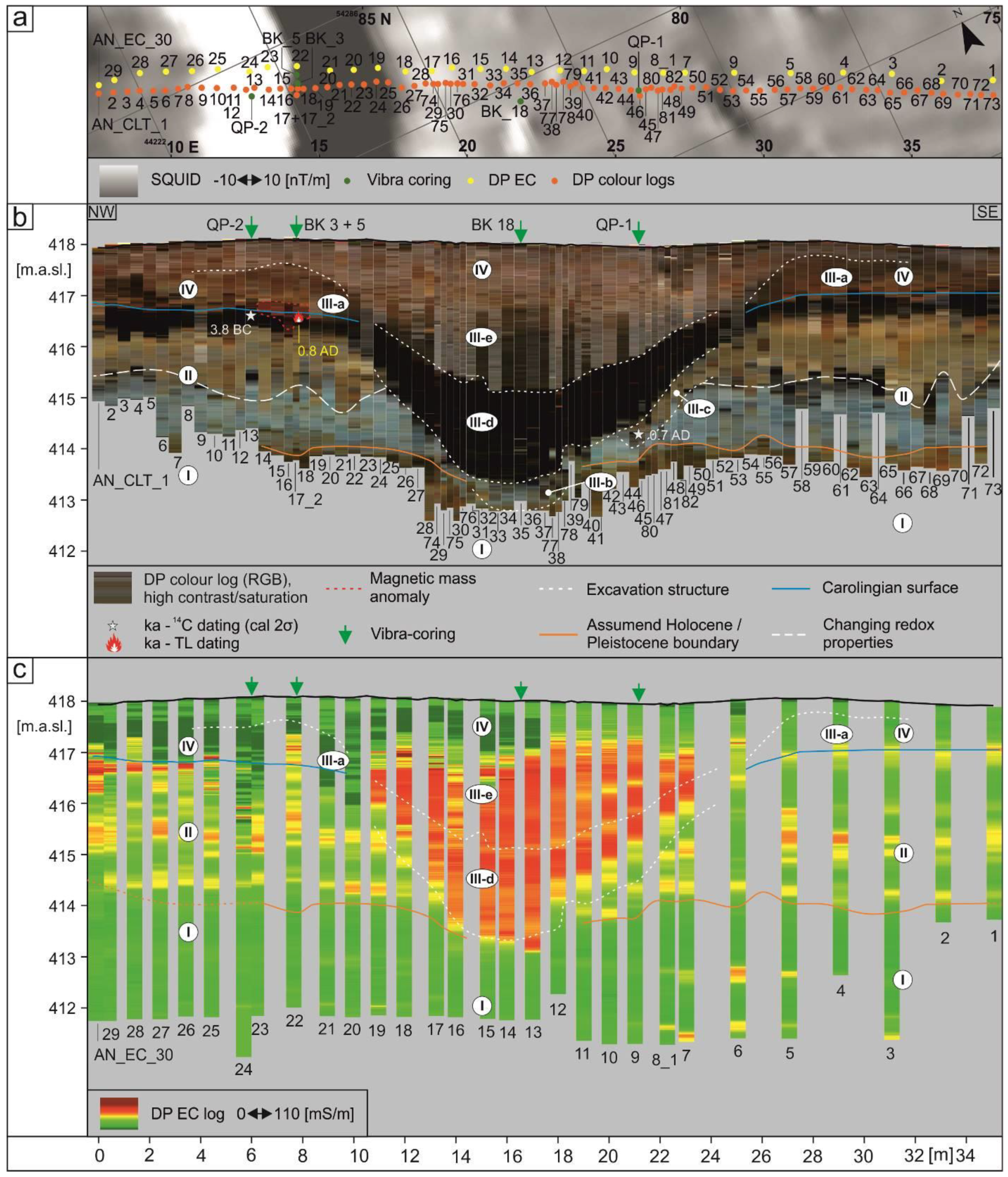
4.1. SQUID Magnetic Survey and Depth Modelling of the Intensive Magnetic Anomaly

The SQUID magnetic survey (Figure 2) reveals a linear and intensive magnetic anomaly that accompanies the canal course. We modelled the depth of the anomaly at six positions by performing approximately 30 depth calculations (see 3.1 Section) out of the SQUID data set (Figure 6). The results range between 1.0 and 1.8 m below the surface. However, most calculations yield similar depth values of approximately 1 m, indicating a persistent subsurface layer in the underground (Figure 6b).

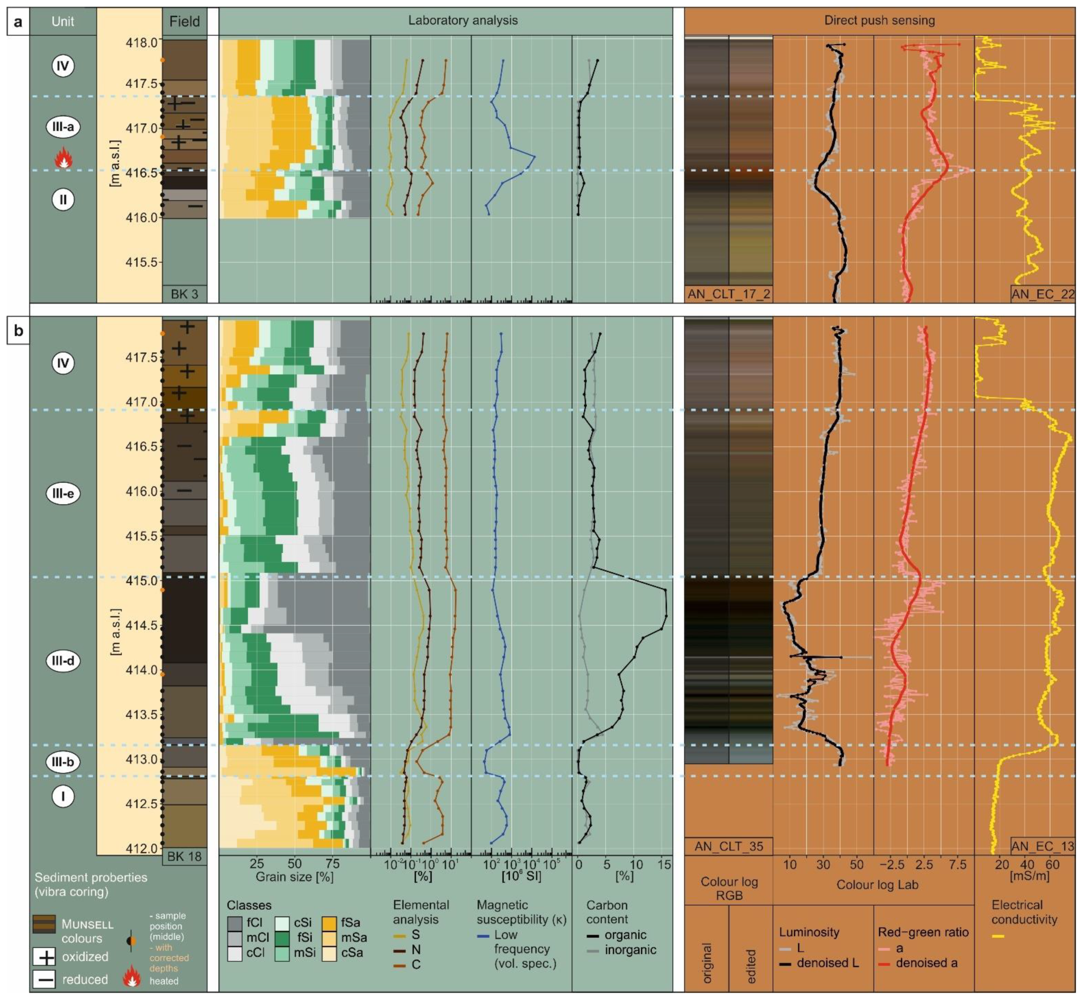
4.2. Chronostratigraphical Units of the Fossa Carolina Cross-Section

We generated a high-resolution 2D cross-section with the direct push colour and electrical conductivity logging as well as vibracoring ground-truthing, which shows different subsurface units in a vertical and lateral direction (Figure 7 and Figure 8 and Table S1 (Supplementary Materials)).

The lowermost Unit I is characterised by brownish colours up to approximately 414 m a.s.l. and shows a horizontally bedded stratigraphy with relatively low electrical conductivities (<20 mS/m). According to core BK18 (412.06–412.96 m a.s.l., Figure 8b), predominantly sandy sediments appear. The CNSand inorganic carbon record is heterogeneous but relatively low and slightly enhanced values of the low-frequency magnetic susceptibility were measured. Furthermore, the unit is nearly plant fragment free. The record was interpreted as sandy valley fills of the Pleistocene or Early Holocene below the canal.

Unit II is characterised by greyish colours in the lower part up to approximately 415 m a.s.l., brownish colours in the upper part, and a dark brown to black layer at approximately 416.5 m a.s.l. It shows a horizontally bedded stratigraphy, with electrical conductivities generally higher (<60 mS/m) than those of Unit I. We drilled vibracoring BK3 at the position of the intensive magnetic anomaly or rather at the margin of the canal structure (Figure 7 and Figure 8a). In Unit II, 416.03–416.57 m a.s.l., we recorded sandy to loamy sediments with several finer-grained layers. The rising values of low-frequency magnetic susceptibility, organic carbon content, and CNS are striking. The values of the Luminosity (L) show bright colours in the lower part and dark colours with minimal values at the transition to the overlying Unit III-a. The cross-section within Unit II shows a reductive–oxidative layering that could have been affected by the groundwater table. The increase in carbon content along with low Luminosity (L) values in the uppermost part indicates a buried topsoil layer. A striking increase in the red–green ratio (a), as well as in low-frequency magnetic susceptibilities, indicate an impact of heating in this zone (Figure 8a). Thus, this layer corresponds with the intensive magnetic anomaly that was detected during the SQUID survey (Figure 2 and Figure 6). The modelled level of approximately 416.9 m a.s.l. is comparable to the elevation of the magnetic mass anomaly at approximately 416.6 m a.s.l. Radiocarbon dating (

Table 1. Stratigraphy position and dating of the fossil topsoil below the magnetic mass anomaly by radiocarbon dating.

Unit	Sample		Sedimentology		Dating
	m a.s.l. (mid)	Sample	Sediment	Feature	Lab No.	Type	Material	14C [yr BP]	13C	cal 2σ
II	416.41	KG-N-QP-2 994 (150–163 cm)	Sandy fluvial deposit (faAh)	Fossil topsoil/magnetic mass anomaly	KIA-50451	14C	Bulk sample	4976 ± 19 BP	−26.2 ± 0.4 ‰	3907–3663 cal BC

) of an organic bulk sample from the fossil topsoil on the level of the magnetic mass anomaly provided a middle Holocene age of the soil formation. For chronological control of the magnetic mass anomaly, we chose to use thermoluminescence dating (TL). The TL dating of the magnetic mass anomaly or, respectively, the dating of the intensively heated sediment (part of Unit II and Unit III-a above) yielded a Carolingian age (

Table 2. Stratigraphic position and dating of the magnetic mass anomaly by thermoluminescence dating. Sample KG-TL2 from the core BK5 (same position as BK3) was intensively heated and provided reliable dating of the magnetic mass anomaly.

Unit	Sample		Sedimentology		Dating
	m a.s.l. (mid)	Sample	Sediment	Feature	Lab No.	Type	Dating	AD/BC
II	416.51	KG2 (BK5 150–155 cm)	Flood loam of the Rezat River	Fossil topsoil/magnetic mass anomaly	MAL 10461	TL	1.21 ± 0.25 ka *	811 ± 250 AD

* related to 2021.

and Table S2, Figure S2).

On top of the buried soil (above Unit II), a dark brownish sediment cover is presented (Unit III-a), which is directly adjacent to the trough structure (Unit III-d and III-e). In the core BK3, Unit III-a (416.57–417.40 m a.s.l.) presents coarser sediments with dark brown to dark yellowish-brown colours (Figure 8a) as well as hydromorphic oxidation and reduction features. CNS and the organic and inorganic carbon content are low. However, low-frequency magnetic susceptibility reaches its maximum at 416.49–416.79 m a.s.l., accompanied by the red–green ratio (a) maximum. The unit displays the sediments of the Carolingian excavation works that are preserved as buried banks; furthermore, the lower part of the unit was impacted by heat. The units are disrupted within the central section (10–24 m on the profile) of the NW–SE transect by inhomogeneous Unit III-b, which shows greyish and brownish colours below 412.9 m a.s.l. In the core BK 18, the Unit III-b (412.96–413.29 m a.s.l.) is characterised by the first appearance of plant fragments (described in the field), whereas the values of CNS and low-frequency magnetic susceptibility are low. The EC-values increase up to >50 mS/m. Along with a slightly fining upward trend, this could represent a first backfill process of bank material.

On the south-eastern side of Unit III-d, a wedge-shaped interruption (Unit III-c) is situated. This represents early backfill sediments as well, which were also radiocarbon dated to Carolingian times (

Table 3. Chronostratigraphy of the canal infill in the northern section by radiocarbon dating from the 2013 excavation—Schnitt 1 [4,77] and vibracoring transects 407 and QP [39].

Unit	Sample			Sedimentology	Chronology	Dating
	m a.s.l. (mid)	Location	Sample/Name			Lab No. (MAMS)	Material	Dating Via	14C [yr BP]	13C	Cal 2σ	Reference
IV (low)	415.81	Excavation	37	Flood loam of the Rezat River	15th–16th century	29839	Seed	Bulk	323 ± 19	−24	AD 1492–1643	[77]
IV (low)	415.6	407	407-1			18374	Charcoal	Core	410 ± 16	−29	AD 1441–1488	[39]
III-e	415.81	Excavation	19	Channel filling: silty-clayey, limnic facies	11th/12th–15th/16th century	29838	Seed	Bulk	959 ± 22	−27	AD 1021–1155	[4]
III-e	415.35		50/51			29846	Seed	Bulk	900 ± 20	−27	AD 1042–1206	[4]
III-d	415.93	Excavation	86	Peat growing/sapropel layer	9th–10th century	29843	Wood	Bulk	1230 ± 20	−25	AD 693–878	[77]
III-d	415.85	Excavation	6	peat growing/sapropel layer	9th–10th century	29837	Wood	Bulk	1228 ± 20	−27	AD 694–879	[77]
III-d	415.34	Excavation	43	First channel fills from excavation	8th–9th century	29840	Wood	Bulk	1099 ± 21	−30	AD 892–990	[77]
III-d	414.89	Excavation	56/58	First channel fills from excavation	8th–9th century	29847	Wood	bulk	1246 ± 20	−26	AD 682–865	[77]
III-d	414.5	Excavation	68	First channel fills from excavation	8th–9th century	29842	Wood	Bulk	1238 ± 21	−25	AD 688–872	[77]
III-d	414.5	Excavation	58	First channel fills from excavation	8th–9th century	29841	Seed	Bulk	1180 ± 21	−29	AD 772–937	[77]
III-d	414.35	Excavation	102	First channel fills from excavation	8th–9th century	29844	Seed	Bulk	1217 ± 20	−28	AD 719–884	[77]
III-d	414.3	Excavation	104	First channel fills from excavation	8th–9th century	29845	Seed	Bulk	1228 ± 23	−27	AD 692–881	[77]
III-b	414.17	QP	QP_1	First channel fills from excavation	8th–9th century	18372	Charcoal	Core	1338 ± 17	−31	AD 650–758	[39]

).

Unit III-d presents a trough-shaped sediment fill, which shows blackish colours up to 415 m a.s.l. as well as dark brown colours up to the top of Unit III-e. In core BK 18 (413.29–415.09 m a.s.l.), Unit III-d consists of organic material with fine-grained clastic sediments that show a fining upward trend and colours between black and dark grey. Furthermore, organic carbon rises to its maximum, which positively correlates with the red–green ratio (a) and inversely with Luminosity (L). The EC values stagnate at approx. 60 mS/m. Further upwards, within Unit III-e (415.09–416.96 m a.sl. in BK18), the grain size becomes coarser, and the colours become brighter, ranging from black to dark yellowish-brown. Hydromorphic oxidation and reduction features appear. The organic carbon strongly decreases, and low-frequency magnetic susceptibility stagnates at a low level. Unit III-d and III-e represent the canal fill, featuring dark-coloured organic-rich sediments from ponding. The much higher EC values (approximately 60 mS/m) in the central part of the cross-section (Unit III-d and III-e) represent relatively fine-grained canal fills. For the chronology of the canal fills (Unit III-d to III-e), published radiocarbon ages were considered (Table 3), which were predominately age controls from the archaeological excavation located at a distance of 270 m to the north [4,30,77]. Accordingly, the peat deposits of Unit III-d and Unit III-e increased over the approximate 200 years after the canal’s construction until approximately 1000 AD. Subsequently, fine-grained sediments were deposited by ponding during the High and Late Middle Ages. These filled up the canal to the level of the fossil topsoil.

The uppermost Unit IV shows brownish colours with suspiciously relatively low electrical conductivities (<30 mS/m). Core BK18 (416.96–417.96 m a.s.l.) and core BK3 (417.40–418.03 m a.s.l.) reveal fine-grained loamy sediments. The values of CNS and low-frequency magnetic susceptibility slightly increase. Unit IV (Table 3 and

Table 4. Chronostratigraphy for the Rezat flood loam (Unit III) above the remains of the Fossa Carolina in the northern section by archaeological dating and dendrochronology (from 2013 excavation—Schnitt 1 [4,77]).

Unit	Sample			Sedimentology	Chronology	Dating Via	Dating	Reference
	m a.s.l. (mid)	Location	Sample/Finding Name		Time Span
IV (up)	-	Excavation	-	Flood loam of the Rezat River	19th–20th century	Findings	Archaeological findings	[4]
IV (mid)	415.75	Excavation	33, 34/35		16th–17th century	Dendrochronology, findings	Dendrochronology 1631 ± 8, horseshoes	[4]
IV (low)	415.81	Excavation	37		15th–16th century	Findings	Ceramic	[77]

) is ubiquitous in the landscape inside as well as outside of the canal, which becomes impressively apparent in the direct push colour transect (Figure 7b). It consists of both alluvial and colluvial sediments deposited since the Late Middle Age, according to archaeological age control. This indicates an intensively used landscape.

5. Discussion

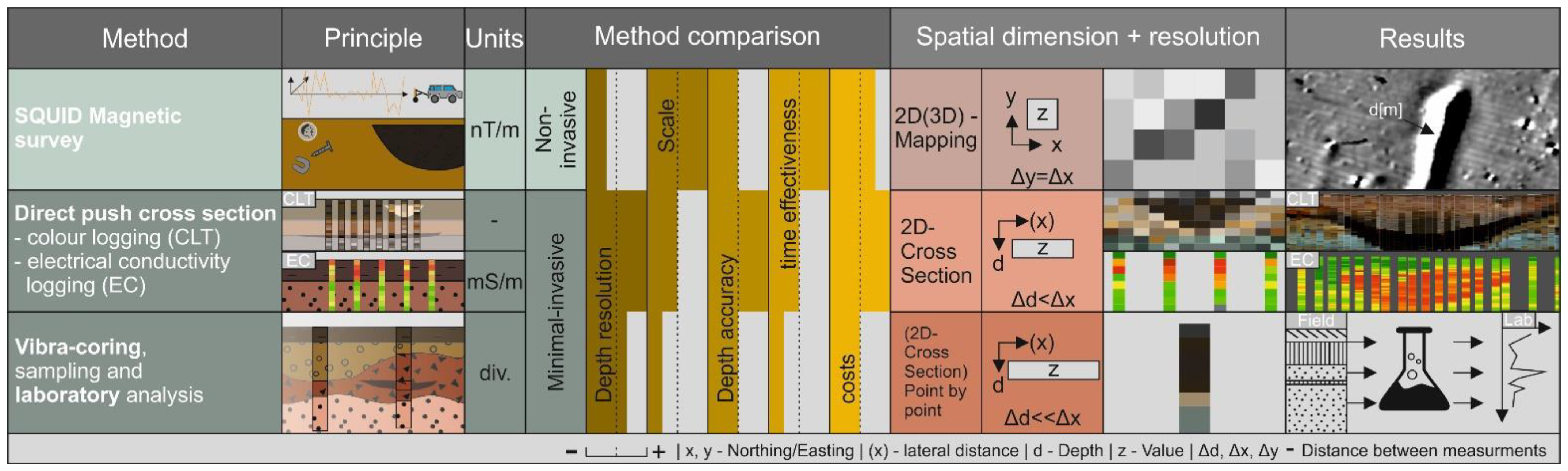
5.1. A Multi-Method Approach with High-Resolution Direct Push Sensing

Non- and minimal-invasive survey methods play an important role in the investigation of archaeological wetland sites when excavations are difficult or undesirable for conservation reasons. Sound approaches require sensitive and complementary methods for the recording of archaeological features at different spatial scales. In this context, we focus on the significance of the results of the SQUID magnetic survey and the high-resolution direct push sensing (Figure 9).

This paper reports on a large-scale magnetic SQUID survey [51] undertaken to identify an archaeological structure (Figure 2), i.e., the large-scale intense magnetic anomaly described above. Further, depths of the magnetic mass anomalies were modelled (Figure 6 and Figure 9) in different segments, offering a third dimension to the data set. This approach has already provided valuable insights concerning circular ditch systems [78], the interpretation of buried walls [79], and potential hydro-engineering structures in the subsurface [16]. The results of magnetic depth modelling allowed the spatial upscaling by tracking the estimated elevation of anomalies in different segments and sections over longer distances (Figure 6). However, this modelling has an uncertainty of several decimetres, so spatial coupling of the intensive magnetic anomaly segments over larger distances could only be approximated. Therefore, ground-truthing was required. Here, direct push sensing yielded high-resolution data concerning buried geoarchaeological structures along both horizontal and vertical axes. Direct push colour logging was utilised to determine the precise position of the magnetic mass anomaly within the stratigraphy of the valley fills and intercalated canal remains (Figure 7). This advanced the previous application of direct push colour logging as point-by-point-insight for the extension of sedimentological descriptions [25,58,80]. Additionally, direct push electrical conductivity sensing resulted in a highly depth-accurate dataset that noticeably improved the spatial significance of common, non-invasive ERT applications e.g., [22,37,81]. Thus, there is a high methodological potential for future combinations of depth-accurate direct push electrical conductivity logging as point-by-point ground-truthing with ERT data sets [17,24,82,83].

Finally, we showed that the selection of a complementary combination of methods (Figure 9) is the key to a reliable multi-method, non- to minimal-invasive approach in wetland geoarchaeology.

5.2. Origin of the Magnetic Mass Anomaly

The SQUID magnetic survey showed an intensive anomaly running parallel to the canal (Figure 6) in the northern and north-eastern sections. Such linear structures in magnetic surveys usually indicate anthropogenic features, e.g., pathways, walls, or ditches [79,84,85]. However, natural linear structures, such as naturally filled gullies, are also known, especially in the vicinity of the Fossa Carolina [16]. The magnetic mass anomaly exhibits a reddish colouring within an intermediate stratigraphical position between the buried mid-Holocene soil (top of Unit II) and the covering Carolingian bank deposits (Unit III-a) (Figure 7b). The TL dating offers a Carolingian age of the heating process. In further segments of the intensive magnetic anomaly, its level was estimated as being close to the former surface of the buried soil (Figure 6). Thus, based on the location and dating, its characterisation as a remnant of the canal construction site is very likely. Due to its stratigraphical position below the excavation material, its formation at a rather early point in the construction process—or at least before digging ended—seems probable.

Besides the red colouring, we know from the rock magnetic analysis [43] that the sediments contain titanomagnetite, which only forms in the presence of very high temperatures (700 °C). It is found primarily in magmatic rocks [86,87] or secondarily as a product of the weathering of basaltic rocks [88]. Neither exists in the area—see [44,45]— which leads to the assumption that it represents an anthropogenic feature.

Furthermore, the red colour might indicate fire exposure, which would also be supported by the rock magnetic analysis. A forest clearing fire at the beginning of the construction work would be a possibility, but these usually only generate temperatures of approximately 300–400 °C [87,88], too low for the formation of titanomagnetite [43]. Furthermore, the heating by fire decreases strongly from the surface to the depth into the sediments [89], which does not fit the red colouration and increased volume magnetic susceptibility over a depth range of approximately 20 cm, which might indicate deep and intense heating. Additionally, there is no evidence for charcoal in the recovered sediments, which could argue against there having been a fire at this place. Another mechanism could be an anthropogenic input of burnt material, e.g., to stabilise a parallel path for the construction site. This could explain the slight embedding (Figure 7b) of the sediments and their width of approximately 2 m (Figure 2), which is similar to the width of towpaths mentioned in other canal studies [90]. Additionally, remains of iron smelting and ceramics from the Early and High Middle Ages were found diffusely distributed during the inspection of adjacent areas [91]. These suggest the occurrence of activities in the near vicinity that might have produced heated sediments without any relation to the canal. However, the SQUID magnetic survey shows discontinuous segments that do not always run in alignment (Figure 2), which speaks against a path. Furthermore, neither ceramic nor iron was found in the recovered sediments of the magnetic mass anomaly.

Thus, we were able to firmly characterise the magnetic mass anomaly as an anthropogenic structure to the Carolingian canal, but we could not present a conclusive interpretation of the sediment of the magnetic mass anomaly.

5.3. New Hints about the Hydro-Engineering Concept and Navigability

Even after numerous studies, questions about the canal summit, water supply, and navigability have not been conclusively answered. The results of this study provide new information about the overall concept.

The direct push colour logs document the canal bottom as being at approximately 413.2 m a.s.l. This is significantly lower than the canal bottom as identified in the 2013 excavation to the north (414.05 m a.s.l. [4]) and significantly higher than the bottom in the west–east section (Figure 1) (approx. 412 m a.s.l. [29]), which is 550 m further southwest (as the crow flies). Hence, there is evidence that the summit of the canal must have been further to the north than previously documented by Zielhofer et al. [39].

The direct push colour logs also provide new insights into the hydro-engineering concept of the canal. The cross-section shows a significant colour change (Figure 7b, Unit II) from greyish colours (below approximately 415 m a.sl.) to yellowish-brown colours (above). This points to the groundwater-dependent reductive and oxidative zone [92] and thus at least to a (semi-stable) groundwater level. Furthermore, the buried organic-rich and boggy topsoil detected at approx. 416.5 m a.s.l. indicate at the very least a semi-terrestrial environment with long-term wet conditions at the Carolingian surface. Since the canal bottom (Unit III-b), at approximately 413.2 m a.s.l., is approximately 1.5–2 m lower than the reductive–oxidative boundary and 3–4 m lower than the organic-rich buried topsoil, an ample groundwater supply at the study site’s canal section would be likely.

Furthermore, the direct push colour cross-section (Figure 7b) provides information on the canal geometry (Unit III-b, III-d and III-e). At the level of approximately 414 m a.s.l. (position AN_CLT_39), an edge appears on the south-eastern side, which points to a lateral or rather vertical boundary of the canal. This might point to oak timber revetments, which are well known from the excavations further north [4]. Using the top level of the timbers as the maximum water elevation (approx. 414 m a.s.l.), the canal has a depth of approximately 1 m and a width of approximately 5 m. This would have been suitable for Carolingian cargo scows [93,94] and therefore suggests navigability in this section. Furthermore, the latter dimension is in line with the computed canal width of approximately 5.2–5.3 m at the excavation site of 2013 [4].

Consequently, our results indicate a navigable section with potential for high groundwater supply that could have fed the summit zone of the Carolingian canal with water. This could be the answer to the lack of water supply structures described in studies [16].

5.4. Construction Site Remains at Early Medieval Buildings

For a large-scale construction site like the Fossa Carolina that involved hundreds or even thousands of workers, one would expect considerable remains of infrastructure and activities in the immediate area of the canal trench. The range of possible remains of the canal construction site covers several functional groups: traces of transportation and mobility infrastructure (e.g., wooden trackways, paved roads, and river crossings), traces of earthworks (e.g., pits and excavated earth), traces of landscape modifications (e.g., drainage ditches, channel engineering, and terrain levelling), traces of processing and craft activities (e.g., activity areas with finds and features associated with carpenters and metalworkers, huts and roofs to provide shelter, lumberyards for timber, and production waste such as wood chips), traces of lodging and supplies for the workforce (e.g., temporary cabins, tents, fireplaces, food waste, and food containers), and traces of surveying (e.g., postholes made by range rods).

The extent and provability of these functional groups are rather different. Due to the scale of the construction site and the wet and boggy conditions, considerable traces of transportation, especially wooden trackways for pedestrian and wheeled transport, seem rather likely. Such trackways, with a typical width of 2–4 m, were typically made of brushwood and hurdle, woven wooden panels, or more advanced timber constructions with transverse logs or planks, substructures, and fillings of sand or peat [95,96]. Early Medieval examples such as the eigth-century wooden trackway in the Klempsau bog (northern Germany), which is contemporary to the Fossa Carolina, feature a stratigraphy of up to 2 m composed of new sand and turf fillings and plank layers, which were placed on top of each other [95]. Archaeological investigation of the 8th century Kanhave canal (Denmark) and the Roman Fossa Corbulonis (Netherlands) have discovered (tow)paths made of artificially filled turf and sods that ran parallel to the canal trench [90,97]. Several other Roman canals feature similar (tow)paths made of wood, earth, and field stones [98,99].

In the immediate area of the Fossa Carolina, one would expect significant traces of processing and craft activities as well as of lodging and supply of the workforce. While the internal organisation of the construction site and workforce are unknown, there are different possibilities. On the one hand, it can be assumed that the village of Graben, located on the south side of the central section (Figure 1), sits on the site of a former construction camp and thus covers its traces. Diffusely distributed Early Medieval iron melting remains and ceramic sherds in the near west–east section could support this supposition [91]. Additionally, the SQUID magnetic survey showed several other anomalies in the canal environment [51] that could indicate traces; these have not yet been investigated. On the other hand, it is possible that tool maintenance, accommodation, and provisioning did not take place in close proximity to the construction site but in surrounding Early Medieval settlements, such as Dettenheim and Weißenburg. These places must have had road communication, storage facilities, and shelter, as well as workshops, such as smitheries [91,100,101,102]. Therefore, it is unsurprising that there are very few archaeological records in this area. Systematic aerial archaeology, fieldwalking, and shovel pit testing in meadows have not yielded noteworthy features or finds such as 8th-century ceramics, iron tools, personal belongings, or any other material remains [37,91,103,104,105]. Furthermore, direct push sensing gives another explanation. The dated Carolingian surface and thus potential findings are covered by an approximately 1 metre-thick layer (Unit IV) of alluvial and colluvial sediments (Figure 7). However, remains of half-finished timbers and diverse wood waste at the bottom of the excavated canal trench point to the fact that at least some portion of the work took place in the trench itself. This might contribute to a lack of surface finds in the surrounding areas [30]. Furthermore, the formation of the archaeological record of the construction site remains is rather complex and the poor preservation of organic objects under aerobic near-surface conditions, as well as their limited recognisability due to colluvial coverage, have to be taken into account [106,107,108].

As we are almost exclusively talking about woodworking and earthwork at the Fossa Carolina, the range of possible archaeological remains outside the construction pit is rather limited. Like the Fossa Carolina and in sharp contrast to sites with evidence of stonemasonry, lime burning, or glassmaking [109,110,111,112,113,114], other large-scale earthworks of the Early Middle Ages such as the Offa’s Dyke, the Danewerk, and the Kanhave canal have yielded a very limited range of finds and features that may be interpreted as construction site remains e.g., [115,116,117].

6. Conclusions

A ground-based, non-invasive, magnetic SQUID survey revealed an intensive and linear magnetic anomaly in the northern section of the Fossa Carolina that cannot be clearly associated with the canal to which the anomaly runs parallel. (i) This paper documents the approach that was used and the specific results that support this contention. First, a minimal-invasive and highly spatial resolved direct push cross-section was conducted using dense colour and electrical conductivity logs with spacings up to 0.25 m. The direct push data were combined with depth-corrected cores, dating, and laboratory analysis. This methodology fills the gap between selective coring activities and large-scale non-invasive geophysical prospection techniques in wetlands. (ii) The magnetic mass anomaly was found to lie directly above the Carolingian surface and below the Carolingian bank deposits. There was evidence that the sediments of the structures had been heated to an extremely high temperature, and TL dating provided a compatible Carolingian age of 811 ± 250 AD. Thus, our study identified verifiable traces of construction activities outside the canal trench itself. For the spatially upscaled interpretation, depth modelling of the anomaly from SQUID data indicates its stratigraphic positioning close to the Carolingian surface level in the northern and north-eastern sections of the canal. This underpins its clear association with the context of the Carolingian canal. Furthermore, we present new indications for a sophisticated hydro-engineering concept of the canal. The direct push data suggest a geometry with a width of approximately 5 m and a depth of approximately 1 m for the waterway and gives hints for an ample groundwater supply in the summit zone of the canal course. We have determined the bottom level of the canal at approximately 413.2 m a.s.l. This is almost 1 m deeper than in the excavated section further north and therefore indicates that the summit of the canal was further north than previously recorded in former studies. Finally, this paper describes a multi-method approach that represents a promising advancement of ground-based non- and minimal-invasive prospection techniques for geoarchaeological investigation and monitoring in wetland environments.

References

1. De Smedt, P.; van Meirvenne, M.; Herremans, D.; de Reu, J.; Saey, T.; Meerschman, E.; Crombé, P.; de Clercq, W. The 3-D reconstruction of medieval wetland reclamation through electromagnetic induction survey. Sci. Rep. 2013, 3, 1517. [Google Scholar] [CrossRef] [Green Version]
2. Verhegge, J.; Storme, A.; Cruz, F.; Crombé, P. Cone penetration testing for extensive mapping of deeply buried Late Glacial coversand landscape paleotopography. Geoarchaeology 2020, 36, 130–148. [Google Scholar] [CrossRef]
3. Werther, L.; Mehler, N.; Schenk, G.J.; Zielhofer, C. On the Way to the Fluvial Anthroposphere—Current Limitations and Perspectives of Multidisciplinary Research. Water 2021, 13, 2188. [Google Scholar] [CrossRef]
4. Werther, L.; Zielhofer, C.; Herzig, F.; Leitholdt, E.; Schneider, M.; Linzen, S.; Berg-Hobohm, S.; Ettel, P.; Kirchner, A.; Dunkel, S. Häfen verbinden. Neue Befunde zu Verlauf, wasserbaulichem Konzept und Verlandung des Karlsgrabens. In Häfen im 1. Millennium AD: Bauliche Konzepte, Herrschaftliche und Religiöse Einflüsse, 1st ed.; Schmidts, T., Vucetic, M., Eds.; Schnell & Steiner: Regensburg, Germany, 2015; ISBN 978-3-88467-249-5. [Google Scholar]
5. Mayr, C.; Matzke-Karasz, R.; Manthe, P.; Arnold, J.; Hänfling, C.; Hilber, J.; Spitzenberger, D.; Schmid, W.; Schönfeld, G. Environmental change in the vicinity of the Neolithic wetland settlement Pestenacker (S-Germany) during the last 6600 years. J. Archaeol. Sci. 2015, 54, 396–409. [Google Scholar] [CrossRef]
6. Menotti, F.; O’Sullivan, A. (Eds.) The Oxford Handbook of Wetland Archaeology, 1st ed.; Oxford University Press: Oxford, UK, 2013; ISBN 9780199573493. [Google Scholar]
7. Bates, M.R.; Bates, C.R. Multidisciplinary Approaches to the Geoarchaeological Evaluation of Deeply Stratified Sedimentary Sequences: Examples from Pleistocene and Holocene Deposits in Southern England, United Kingdom. J. Archaeol. Sci. 2000, 27, 845–858. [Google Scholar] [CrossRef]
8. Werther, L.; Feiner, D. Der Karlsgraben im Fokus der Archäologie. In Großbaustelle 793: Das Kanalprojekt Karls des Großen zwischen Rhein und Donau; Ettel, P., Daim, F., Berg-Hobohm, S., Werther, L., Zielhofer, C., Eds.; Verlag des Römisch-Germanischen Zentralmuseums: Mainz, Germany, 2014; pp. 33–40. ISBN 978-3-88467-232-7. [Google Scholar]
9. Zielhofer, C.; Rabbel, W.; Wunderlich, T.; Vött, A.; Berg, S. Integrated geophysical and (geo)archaeological explorations in wetlands. Quat. Int. 2018, 473, 1–2. [Google Scholar] [CrossRef]
10. Caple, C. Reburial of Waterlogged Wood, The problems and Potential of this Conservation Technique. Inter. Biodeter. Biodegr. 1994, 34, 61–72. [Google Scholar] [CrossRef]
11. Cronyn, J.M. The Elements of Archaeological Conservation; Reprint; Routledge: London, UK, 2005; ISBN 0-415-01207-4. [Google Scholar]
12. Drahor, M.G. Integrated geophysical studies in the upper part of Sardis archaeological site, Turkey. J. Appl. Geophy. 2006, 59, 205–223. [Google Scholar] [CrossRef]
13. Kvamme, K.L. Geophysical Surveys as Landscape Archaeology. Am. Antiq. 2003, 68, 435–457. [Google Scholar] [CrossRef]
14. Viberg, A.; Trinks, I.; Lidén, K. A Review of the Use of Geophysical Archaeological Prospection in Sweden. Archaeol. Prospect. 2011, 18, 43–56. [Google Scholar] [CrossRef]
15. Dalan, R.A.; Banerjee, S.K. Solving Archaeological Problems using Techniques of Soil Magnetism. Geoarchaeology 1998, 13, 3–36. [Google Scholar] [CrossRef]
16. Rabiger-Völlmer, J.; Schmidt, J.; Linzen, S.; Schneider, M.; Werban, U.; Dietrich, P.; Wilken, D.; Wunderlich, T.; Fediuk, A.; Berg, S.; et al. Non-invasive prospection techniques and direct push sensing as high-resolution validation tools in wetland geoarchaeology—Artificial water supply at a Carolingian canal in South Germany? J. Appl. Geophy. 2020, 173, 103928. [Google Scholar] [CrossRef]
17. Wunderlich, T.; Fischer, P.; Wilken, D.; Hadler, H.; Erkul, E.; Mecking, R.; Günther, T.; Heinzelmann, M.; Vött, A.; Rabbel, W. Constraining electric resistivity tomography by direct push electric conductivity logs and vibracores: An exemplary study of the Fiume Morto silted riverbed (Ostia Antica, western Italy). Geophysics 2018, 83, B87–B103. [Google Scholar] [CrossRef]
18. Döberl, G.; Müller, D.; Dörrie, T. Guideline: Section 1. In Model-Driven Soil Probing, Site Assessment and Evaluation: Guidance on Technologies; Kästner, M., Braeckevelt, M., Döberl, G., Cassiani, G., Papini, M.P., Leven-Pfister, C., van Ree, D., Eds.; Sapienza Universita Editrice: Roma, Italy, 2012; ISBN 978-88-95814-7-28. [Google Scholar]
19. Boucher, A.R. Archaeological Feedback in Geophysics. Archaeol. Prospect. 1996, 3, 129–140. [Google Scholar] [CrossRef]
20. Schrott, L.; Sass, O. Application of field geophysics in geomorphology: Advances and limitations exemplified by case studies. Geomorphology 2008, 93, 55–73. [Google Scholar] [CrossRef]
21. Armstrong, K.; Cheetham, P.; Darvill, T. Tales from the outer limits: Archaeological geophysical prospection in lowland peat environments in the British Isles. Archaeol. Prospect. 2019, 26, 91–101. [Google Scholar] [CrossRef] [Green Version]
22. Carey, C.; Howard, A.J.; Jackson, R.; Brown, A. Using geoarchaeological deposit modelling as a framework for archaeological evaluation and mitigation in alluvial environments. J. Archaeol. Sci. Rep. 2017, 11, 658–673. [Google Scholar] [CrossRef]
23. Leitholdt, E.; Zielhofer, C.; Berg-Hobohm, S.; Schnabl, K.; Kopecky-Hermanns, B.; Bussmann, J.; Härtling, J.W.; Reicherter, K.; Unger, K. Fossa Carolina: The First Attempt to Bridge the Central European Watershed-A Review, New Findings, and Geoarchaeological Challenges. Geoarchaeology 2012, 27, 88–104. [Google Scholar] [CrossRef]
24. Fischer, P.; Wunderlich, T.; Rabbel, W.; Vött, A.; Willershäuser, T.; Baika, K.; Rigakou, D.; Metallinou, G. Combined Electrical Resistivity Tomography (ERT), Direct-Push Electrical Conductivity (DP-EC) Logging and Coring—A New Methodological Approach in Geoarchaeological Research. Archaeol. Prospect. 2016, 23, 213–228. [Google Scholar] [CrossRef]
25. Verhegge, J.; Crombé, P.; van den Wijngaert, M. Prehistoric landscape mapping along the Scheldt by camera- and conductivity CPT-E. In Cone Penetration Testing 2018, Proceedings of the 4th International Symposium on Cone Penetration Testing (CPT’18), Delft, The Netherlands, 21–23 June 2018; Hicks, M., Pisanò, F., Peuchen, J., Eds.; CRC Press: Boca Raton, FL, USA, 2018; ISBN 9780429000485. [Google Scholar]
26. Hausmann, J.; Zielhofer, C.; Werther, L.; Berg-Hobohm, S.; Dietrich, P.; Heymann, R.; Werban, U. Direct push sensing in wetland (geo)archaeology: High-resolution reconstruction of buried canal structures (Fossa Carolina, Germany). Quat. Int. 2018, 473, 21–36. [Google Scholar] [CrossRef]
27. Dietrich, P.; Leven, C. Direct pushtechnologies. In Groundwater Geophysics: A Tool for Hydrogeology, 2nd ed.; Kirsch, R., Ed.; Springer: Berlin/Heidelberg, Germany, 2009; pp. 347–366. ISBN 978-3-540-88404-0. [Google Scholar]
28. Bumberger, J.; Paasche, H.; Dietrich, P. Systematic description of direct push sensor systems: A conceptual framework for system decomposition as a basis for the optimal sensor system design. J. Appl. Geophy. 2015, 122, 210–217. [Google Scholar] [CrossRef]
29. Völlmer, J.; Zielhofer, C.; Hausmann, J.; Dietrich, P.; Werban, U.; Schmidt, J.; Werther, L.; Berg, S. Minimalinvasive Direct-push-Erkundung in der Feuchtboden(geo)archäologie am Beispiel des Karlsgrabens (Fossa Carolina). Archaol. Korresp. 2018, 48, 577–593. [Google Scholar]
30. Werther, L.; Nelson, J.; Herzig, F.; Schmidt, J.; Berg, S.; Ettel, P.; Linzen, S.; Zielhofer, C. 792 or 793? Charlemagne’s canal project: Craft, nature and memory. Early Mediev. Eur. 2020, 28, 444–465. [Google Scholar] [CrossRef]
31. Hack, A. Der Bau des Karlsgrabens nach den Schriftquellen. In Großbaustelle 793: Das Kanalprojekt Karls des Großen Zwischen Rhein und Donau; Ettel, P., Daim, F., Berg-Hobohm, S., Werther, L., Zielhofer, C., Eds.; Verlag des Römisch-Germanischen Zentralmuseums: Mainz, Germany, 2014; pp. 53–62. ISBN 978-3-88467-232-7. [Google Scholar]
32. Nelson, J. Evidence in question: Dendrochronology and early medieval historians. In Entre Texte et Histoire: Études d’histoire Médiévale Offertes au Professeur Shoichi Sato; Kanō, O., Lemaître, J.-L., Eds.; De Boccard: Paris, France, 2015; pp. 227–249. ISBN 9782701804514. [Google Scholar]
33. Zielhofer, C.; Kirchner, A. Naturräumliche Gunstlage der Fossa Carolina. In Großbaustelle 793: Das Kanalprojekt Karls des Großen zwischen Rhein und Donau; Ettel, P., Daim, F., Berg-Hobohm, S., Werther, L., Zielhofer, C., Eds.; Verlag des Römisch-Germanischen Zentralmuseums: Mainz, Germany, 2014; pp. 5–8. ISBN 978-3-88467-232-7. [Google Scholar]
34. Werther, L.; Berg, S.; Ettel, P.; Schmidt, J.; Zielhofer, C. Fossa Carolina/Karlsgraben. Available online: http://www.historisches-lexikon-bayerns.de/Lexikon/Fossa_Carolina_/_Karlsgraben (accessed on 28 June 2019).
35. Schmidt, J.; Werther, L.; Zielhofer, C. Shaping Pre-Modern Digital Terrain Models: The Former Topography at Charlemagne’s Canal Construction Site. PLoS ONE 2018, 13, e0200167. [Google Scholar] [CrossRef] [PubMed]
36. Schmidt, J.; Werther, L.; Rabiger-Völlmer, J.; Herzig, F.; Schneider, B.; Werban, U.; Dietrich, P.; Berg, S.; Linzen, S.; Ettel, P.; et al. Sediment budgeting of short-term backfilling processes: The erosional collapse of a Carolingian canal construction. Earth Surf. Process. Landf. 2020, 45, 3449–3462. [Google Scholar] [CrossRef]
37. Kirchner, A.; Zielhofer, C.; Werther, L.; Schneider, M.; Linzen, S.; Wilken, D.; Wunderlich, T.; Rabbel, W.; Meyer, C.; Schmidt, J.; et al. A multidisciplinary approach in wetland geoarchaeology: Survey of the missing southern canal connection of the Fossa Carolina (SW Germany). Quat. Int. 2018, 473, 3–20. [Google Scholar] [CrossRef]
38. Leitholdt, E.; Krüger, A.; Zielhofer, C. The medieval peat layer of the Fossa Carolina—Evidence for bridging the Central European Watershed or climate control? Z. Geomorphol. Suppl. 2014, 58, 189–209. [Google Scholar] [CrossRef]
39. Zielhofer, C.; Leitholdt, E.; Werther, L.; Stele, A.; Bussmann, J.; Linzen, S.; Schneider, M.; Meyer, C.; Berg-Hobohm, S.; Ettel, P.; et al. Charlemagne’s Summit Canal: An Early Medieval Hydro-Engineering Project for Passing the Central European Watershed. PLoS ONE 2014, 9, e108194. [Google Scholar] [CrossRef]
40. Berg-Hobohm, S.; Werther, L. Das rezente Erschinungsbild des Karlsgrabens. In Großbaustelle 793: Das Kanalprojekt Karls des Großen zwischen Rhein und Donau; Ettel, P., Daim, F., Berg-Hobohm, S., Werther, L., Zielhofer, C., Eds.; Verlag des Römisch-Germanischen Zentralmuseums: Mainz, Germany, 2014; pp. 9–12. ISBN 978-3-88467-232-7. [Google Scholar]
41. European Environment Agency. European River Catchments: Zipped Shapefile, Vector Polygon, 2008, Shapefile extracted from the ERC110708F1v1 geodatabase. 2008. Available online: https://www.eea.europa.eu/data-and-maps/data/european-river-catchments-1 (accessed on 29 June 2020).
42. Linzen, S.; Schneider, M. Der Karlsgraben im Fokus der Geophysik. In Großbaustelle 793: Das Kanalprojekt Karls des Großen zwischen Rhein und Donau; Ettel, P., Daim, F., Berg-Hobohm, S., Werther, L., Zielhofer, C., Eds.; Verlag des Römisch-Germanischen Zentralmuseums: Mainz, Germany, 2014; pp. 29–32. ISBN 978-3-88467-232-7. [Google Scholar]
43. Stele, A.; Fassbinder, J.W.E.; Härtling, J.W.; Bussmann, J.; Schmidt, J.; Zielhofer, C. Genesis of magnetic anomalies and magnetic properties of archaeological sediments in floodplain wetlands of the Fossa Carolina. Archaeol. Prospect. 2019, 4, 113. [Google Scholar] [CrossRef]
44. Berger, K.; Schmidt-Kaler, H. Geologische Karte von Bayern 6931 Weißenburg: 1:25,000; Bayerisches Landesamt für Umwelt: Augsburg, Germany, 1982. [Google Scholar]
45. Schmidt-Kaler, H. Geologische Karte von Bayern 7031 Treuchtlingen: 1:25,000; Bayerisches Landesamt für Umwelt: Augsburg, Germany, 1976. [Google Scholar]
46. Zielhofer, C. Hydrographical and hydrochemical characteristics of karst water components (southern Franconian Jura)–a contribution to fresh water protection and karst morphogenesis. Z. Geomorphol. Suppl. 2004, 136, 113–134. [Google Scholar]
47. Lietz, K. Hydrogeochemische Analyse des Einzugsgebietes der Schwäbischen Rezat im Siechten Karst der Südlichen Frankenalb. Master’s Thesis, Institute of Geography, Leipzig University, Leipzig, Germany, 2014, unpublished. [Google Scholar]
48. Linzen, S.; Chwala, A.; Schultze, V.; Schulz, M.; Schüler, T.; Stolz, R.; Bondarenko, N.; Meyer, H.-G. A LTS-SQUID System for Archaeological Prospection and Its Practical Test in Peru. IEEE Trans. Appl. Supercond. 2007, 17, 750–755. [Google Scholar] [CrossRef]
49. Linzen, S.; Schultze, V.; Chwala, A.; Schüler, T.; Schulz, M.; Stolz, R.; Meyer, H.-G. Quantum Detection Meets Archaeology—Magnetic Prospection with SQUIDs, Highly Sensitive and Fast. In New Technologies for Archaeology: Multidisciplinary Investigations in Palpa and Nasca, Peru; Herrmann, B., Reindel, M., Wagner, G.A., Eds.; Springer: Berlin/Heidelberg, Germany, 2009; pp. 71–85. ISBN 978-3-540-87437-9. [Google Scholar]
50. Berg-Hobohm, S.; Fassbinder, J.W.E.; Linzen, S. Neue Forschungsergebnisse am Karlsgraben durch geophysikalische Messmethoden. Denkmalpf. Inf. 2014, 25–27. [Google Scholar]
51. Linzen, S.; Schneider, M.; Berg-Hobohm, S.; Werther, L.; Ettel, P.; Zielhofer, C.; Schmidt, J.; Fassbinder, J.W.E.; Wilken, D.; Fediuk, A.; et al. From magnetic SQUID prospection to excavation—investigations at Fossa Carolina, Germany. In 12th International Conference of Archaeological Prospection, University of Bradford, Bradford, UK, 12–16 September 2017; Jennings, B., Gaffney, C., Sparrow, T., Gaffney, S., Eds.; Archaeopress: Oxford, UK, 2017; pp. 144–145. ISBN 1784916773. [Google Scholar]
52. Schneider, M.; Linzen, S.; Schiffler, M.; Pohl, E.; Ahrens, B.; Dunkel, S.; Stolz, R.; Bemmann, J.; Meyer, H.-G.; Baumgarten, D. Inversion of Geo-Magnetic SQUID Gradiometer Prospection Data Using Polyhedral Model Interpretation of Elongated Anomalies. IEEE Trans. Magn. 2014, 50, 1–4. [Google Scholar] [CrossRef]
53. Schneider, M.; Stolz, R.; Linzen, S.; Schiffler, M.; Chwala, A.; Schulz, M.; Dunkel, S.; Meyer, H.-G. Inversion of geo-magnetic full-tensor gradiometer data. J. Appl. Geophy. 2013, 92, 57–67. [Google Scholar] [CrossRef]
54. Schultze, V.; Linzen, S. Device and Method for Mapping of Sources for the Local Variation of the Earth’s Magnetic Field. German Patent Application DE 10 2007 030 481.3, 2007. [Google Scholar]
55. Leven, C.; Weiß, H.; Vienken, T.; Dietrich, P. Direct-Push-Technologien—Effiziente Untersuchungsmethoden für die Untergrunderkundung. Grundwasser 2011, 16, 221–234. [Google Scholar] [CrossRef]
56. Hartemink, A.E.; Minasny, B. Towards digital soil morphometrics. Geoderma 2014, 230–231, 305–317. [Google Scholar] [CrossRef]
57. CIE. CIE 15: Technical Report: Colorimetry, 3rd ed.; CIE Central Bureau: Vienna, Austria, 2004; ISBN 3901906339. [Google Scholar]
58. Hausmann, J.; Dietrich, P.; Vienken, T.; Werban, U. Technique, analysis routines, and application of direct push-driven in situ color logging. Environ. Earth. Sci. 2016, 75, 1–21. [Google Scholar] [CrossRef]
59. Beck, F.P.; Clark, P.J.; Puls, R.W. Location and Characterization of Subsurface Anomalies Using a Soil Conductivity Probe. Ground Water Monit. Remediat. 2000, 20, 55–59. [Google Scholar] [CrossRef]
60. Christy, C.D.; Christy, T.M.; Wittig, V. A percussion probing tool for the direct sensing of soil conductivity. In Proceedings of the 8th National Outdoor Action Conference, Washington, DC, USA, 23–25 May 1994; pp. 381–394. [Google Scholar]
61. Schulmeister, M.K. High-resolution Stratigraphic Characterization of Unconsolidated Deposits Using Direct-push Electrical Conductivity Logging: A floodplain-margin example. In Aquifer characterization; Bridge, J.S., Ed.; SEPM: Tulsa, OK, USA, 2004; pp. 67–78. ISBN 1-56576-107-3. [Google Scholar]
62. Butler, J.J.; Healey, J.M.; Zheng, L.; McCall, G.W.; Schulmeister, M.K. Hydrostratigraphic Characterization of Unconsolidated Alluvial Deposits with Direct-push Sensor Technology; Kansas Geological Survey Open-File Report; Kansas Geological Survey: Lawrence, KS, USA, 1999; Volume 99, p. 40. [Google Scholar]
63. McCall, G.W. Electrical conductivity logging to determine control of hydrocarbon flow paths in alluvial sediments. In Proceedings of the 10th National Outdoor Action Conference, Sydney, Australia, 13–15 May 1996; pp. 461–477. [Google Scholar]
64. Schulmeister, M.K.; Butler, J.J.; Healey, J.M.; Zheng, L.; Wysocki, D.A.; McCall, G.W. Direct-push Electrical Conductivity Logging for High-Resolution Hydrostratigraphic Characterization. Ground Water Monit. Remediat. 2003, 23, 52–62. [Google Scholar] [CrossRef]
65. Ad-Hoc-AG Boden. Bodenkundliche Kartieranleitung. KA5; Schweizerbart Science Publishers: Stuttgart, Germany, 2006; ISBN 9783510959204. [Google Scholar]
66. Munsell. Munsell Soil Color Charts; Macbeth Division of Kollmorgen Instruments Corporation: New Windsor, NY, USA, 1994. [Google Scholar]
67. Bartington Instruments. MS3 Magnetic Susceptibility Meter; Bartington Instruments Limited: Oxford, UK, 2000. [Google Scholar]
68. Dearing, J.A. Environmental Magnetic Susceptibility: Using the Bartington MS2 System; Chi Publishing: Kenilworth, UK, 1999; ISBN 0952340909. [Google Scholar]
69. Richter, D.; Mercier, N.; Valladas, H.; Jaubert, J.; Texier, P.-J.; Brugal, J.-P.; Kervazo, B.; Reyss, J.-L.; Joron, J.-L.; Wagner, G.A. Thermoluminescence dating of heated flint from the Mousterian site of Bérigoule, Murs, Vaucluse, France. J. Archaeol. Sci. 2007, 34, 532–539. [Google Scholar] [CrossRef]
70. von Suchodoletz, H.; Blanchard, H.; Hilgers, A.; Radtke, U.; Fuchs, M.; Dietze, M.; Zöller, L. TL and ESR dating of Middle Pleistocene lava flows on Lanzarote island, Canary Islands (Spain). Quat. Geochronol. 2012, 9, 54–64. [Google Scholar] [CrossRef]
71. Anderson, S.L.; Feathers, J.K. Applying luminescence dating of ceramics to the problem of dating Arctic archaeological sites. J. Archaeol. Sci. 2019, 112, 105030. [Google Scholar] [CrossRef]
72. Aitken, M.J. Thermoluminescence Dating; Academic Press: London, UK, 1985; ISBN 0120463814. [Google Scholar]
73. Prescott, J.R.; Hutton, J.T. Cosmic ray and gamma ray dosimetry for TL and ESR. Int. J. Radiat. Appl. Instrum. Part D Nucl. Tracks Radiat. Meas. 1988, 14, 223–227. [Google Scholar] [CrossRef]
74. Synal, H.-A.; Stocker, M.; Suter, M. MICADAS: A new compact radiocarbon AMS system. Nucl. Instrum. Methods Phys. Res. B 2007, 259, 7–13. [Google Scholar] [CrossRef]
75. Podaru, N.C.; Gottdang, A.; Mous, D.J.W.; McDaniel, F.D.; Doyle, B.L. Design and Performance Of A 3 MV Tandetron™ Accelerator System For High-Current Applications. In Application of Accelerators in Research and Industry, Proceedings of the Twenty-First International Conference, AIP Conference Proceedings, Fort Worth, TX, USA, 8–13 August 2010; Del McDaniel, F., Doyle, B.L., Eds.; AIP: New York, NY, USA, 2011; Volume 1336, pp. 56–59. ISBN 0735408912. [Google Scholar]
76. Reimer, P.J.; Bard, E.; Bayliss, A.; Beck, J.W.; Blackwell, P.G.; Ramsey, C.B.; Buck, C.E.; Cheng, H.; Edwards, R.L.; Friedrich, M.; et al. IntCal13 and Marine13 Radiocarbon Age Calibration Curves 0–50,000 Years cal BP. Radiocarbon 2013, 55, 1869–1887. [Google Scholar] [CrossRef] [Green Version]
77. Werther, L. Der Karlsgraben und Andere Kanalbauten als Schnittstellen Frühgeschichtlicher Verkehrsnetzwerke. Habilitation Thesis, Jena University, Jena, Germany, 2020. [Google Scholar]
78. Neubauer, W.; Eder-Hinterleitner, A. 3D-Interpretation of Postprocessed Archaeological Magnetic Prospection Data. Archaeol. Prospect. 1997, 4, 191–205. [Google Scholar] [CrossRef]
79. Bescoby, D.J.; Cawley, G.C.; Chroston, P.N. Enhanced Interpretation of Magnetic Survey Data Using Artificial Neural Networks: A Case Study from Butrint, Southern Albania. Archaeol. Prospect. 2004, 11, 189–199. [Google Scholar] [CrossRef]
80. Dalan, R.A.; Bevan, B.W.; Goodman, D.; Lynch, D.; de Vore, S.; Adamek, S.; Martin, T.; Holley, G.; Michlovic, M. The Measurement and Analysis of Depth in Archaeological Geophysics: Tests at the Biesterfeldt Site, USA. Archaeol. Prospect. 2011, 18, 245–265. [Google Scholar] [CrossRef]
81. Altmeyer, M.; Seeliger, M.; Ginau, A.; Schiestl, R.; Wunderlich, J. Reconstruction of former channel systems in the northwestern Nile Delta (Egypt) based on corings and electrical resistivity tomography (ERT). E&G Quat. Sci. J. 2021, 70, 151–164. [Google Scholar] [CrossRef]
82. Corradini, E.; Dreibrodt, S.; Erkul, E.; Groß, D.; Lübke, H.; Panning, D.; Pickartz, N.; Thorwart, M.; Vött, A.; Willershäuser, T.; et al. Understanding Wetlands Stratigraphy: Geophysics and Soil Parameters for Investigating Ancient Basin Development at Lake Duvensee. Geosciences 2020, 10, 314. [Google Scholar] [CrossRef]
83. Verhegge, J.; Missiaen, T.; Crombé, P. Exploring Integrated Geophysics and Geotechnics as a Paleolandscape Reconstruction Tool: Archaeological Prospection of (Prehistoric) Sites Buried Deeply below the Scheldt Polders (NW Belgium). Archaeol. Prospect. 2016, 23, 125–145. [Google Scholar] [CrossRef]
84. Rabbel, W.; Stuempel, H.; Woelz, S. Archeological prospecting with magnetic and shear-wave surveys at the ancient city of Miletos (western Turkey). Lead. Edge 2004, 23, 690–703. [Google Scholar] [CrossRef]
85. Fassbinder, J.W.E. Geophysical prospection of the frontiers of the Roman Empire in southern Germany, UNESCO World Heritage Site. Archaeol. Prospect. 2010, 17, 129–139. [Google Scholar] [CrossRef]
86. Schön, J.H. Physical Properties of Rocks: A Workbook; Elsevier Science: Amsterdam, The Netherlands, 2011; ISBN 978-0-444-53796-6. [Google Scholar]
87. Cornell, R.M.; Schwertmann, U. The Iron Oxides: Structure, Properties, Reactions, Occurences and Uses; 2nd completely revised and extended ed; Wiley-VCH: Weinheim, Germany, 2003; ISBN 3527302743. [Google Scholar]
88. Fassbinder, J.W.E.; Bondar, K. Geophysikalische Prospektion und magnetische Eigenschaften von ausgewählten Böden der Osterinsel. ZAAK 2013, 5, 113–140. [Google Scholar]
89. Canti, M.G.; Linford, N. The Effects of Fire on Archaeological Soils and Sediments: Temperature and Colour Relationships. Proc. Prehist. Soc. 2000, 66, 385–395. [Google Scholar] [CrossRef]
90. de Kort, J.-W.; Raczynski-Henk, Y. The Fossa Corbulonis between the Rhine and Meuse estuaries in the Western Netherlands. In Roman Canals Studies; Salomon, F., Purdue, L., Goiran, J.-P., Berger, J.-F., Eds.; Water History; Springer: Cham, Switzerland, 2014; Volume 6, pp. 51–71. [Google Scholar] [CrossRef]
91. Werther, L. Siedlungsentwicklung und Kulturlandschaft im Umfeld des Karlsgrabens. In Großbaustelle 793: Das Kanalprojekt Karls des Großen zwischen Rhein und Donau; Ettel, P., Daim, F., Berg-Hobohm, S., Werther, L., Zielhofer, C., Eds.; Verlag des Römisch-Germanischen Zentralmuseums: Mainz, Germany, 2014; pp. 45–52. ISBN 978-3-88467-232-7. [Google Scholar]
92. Blume, H.-P.; Brümmer, G.W.; Horn, R.; Kandeler, E.; Kögel-Knabner, I.; Kretzschmar, R.; Stahr, K.; Thiele-Bruhn, S.; Welp, G.; Wilke, B.-M. Scheffer/Schachtschabel Lehrbuch der Bodenkunde, 16th ed.; Spektrum: Berlin, Germany, 2010; ISBN 9783827414441. [Google Scholar]
93. Hoffman, P.; Ellmers, D. Ein Frachter aus der Zeit Karls des Großen. Bremer Archäologische Blätter 1990, 33–37. [Google Scholar]
94. Bockius, R. Binnenfahrzeuge im Karolingerreich. In Großbaustelle 793: Das Kanalprojekt Karls des Großen zwischen Rhein und Donau; Ettel, P., Daim, F., Berg-Hobohm, S., Werther, L., Zielhofer, C., Eds.; Verlag des Römisch-Germanischen Zentralmuseums: Mainz, Germany, 2014; pp. 81–86. ISBN 978-3-88467-232-7. [Google Scholar]
95. Stark, J. Der frühslawische Bohlenweg im Klempauer Moor, Hansestadt Lübeck, und der Burgwall von Klempau, Kreis Herzogtum Lauenburg. In Warentransport im Mittelalter und in der frühen Neuzeit: Transportwege—Transportmittel—Infrastruktur; Wemhoff, M., Ed.; Mitteilungen der Deutschen Gesellschaft für Archäologie des Mittelalters und der Neuzeit; Deutsche Gesellschaft für Archäologie des Mittelalters und der Neuzeit: Paderborn, Germany, 2003; pp. 85–91. [Google Scholar]
96. Brunning, R.; McDermott, C. Trackways and Roads across the Wetlands. In The Oxford Handbook of Wetland Archaeology, 1st ed.; Menotti, F., O’Sullivan, A., Eds.; Oxford University Press: Oxford, UK, 2013; pp. 359–384. ISBN 9780199573493. [Google Scholar]
97. Nørgård Jørgensen, A. Naval Bases in Southern Scandinavia from the 7th to the 12th Century. In Maritime Warfare in Northern Europe: Technology, Organisation, Logistics and Administration 500 BC-1500 AD.; Nørgård Jørgensen, A., Pind, J., Jørgensen, L., Clausen, B., Eds.; PNM Publications from The National Museum: Copenhagen, Denmark, 2002; pp. 125–152. ISBN 8789384881. [Google Scholar]
98. Bonnet, F. Le canal romain d’Avenches. Rapport sur les fouilles exécutées en 1980 et 1981. Bull. L’association Pro Aventico 1982, 27, 3–56. [Google Scholar]
99. Pichon, M. Le transport par voie navigable. L’exemple du site de Tendu (Indre). Carrières antiques de la Gaule: Dossier; CNRS éditions: Paris, France, 2002; pp. 83–88. ISBN 227106063X. [Google Scholar]
100. Hofmann, H.H. Fossa Carolina: Versuch einer Zusammenschau. In Lebenswerk und Nachleben. Karl der Große; Braunfels, W., Ed.; publisher: Düsseldorf, Germany, 1965; pp. 437–453. [Google Scholar]
101. Eigler, F. Weißenburg und sein Umland im Jahre 793.: Villa nostra. In Weißenburger Blätter für Geschichte, Heimatkunde und Kultur von Stadt und Weißenburger Land; Villa Nostra: Beringen, Belgium, 1993; Volume 2, pp. 5–23. [Google Scholar]
102. Beck, M.; Merthen, C. Zwischen Hain und Himmelreich: Die Reihengräber von Weißenburg; Veröffentlichungen Des Frankenbundes, Gr. Weißenburg Bayern; Frankenbundes Gruppe Weißenburg e.V.: Weißenburg, Germany, 2013; p. 57. [Google Scholar]
103. Globig, P. Luftbildarchäologische Untersuchungen im Umfeld des Karlsgrabens. Bachlor’s Thesis, Jena University, Jena, Germany, 2014, unpublished. [Google Scholar]
104. Koch, R. Das archäologische Umfeld der Fossa Carolina. Kölner Jahrb. Für Vor- U. Frühgeschichte 1990, 23, 669–678. [Google Scholar]
105. Ruchte, T.; Schulz, L.; Werther, L. Landnutzung und Siedlungsentwicklung im Umfeld des Karlsgrabens. Scherbenschleier als Archäologische Quelle. Available online: http://archaeologik.blogspot.de/2015/11/landnutzung-und-siedlungsentwicklung-im.html (accessed on 11 February 2019).
106. Sommer, U. Zur Entstehung archäologischer Fundvergesellschaftungen: Versuch einer archäologischen Taphonomie. In Die geographische Ausrichtung bandkeramischer Häuser; Mattheusser, E., Ed.; Habelt: Bonn, Germany, 1991; ISBN 3-7749-2526-7. [Google Scholar]
107. Schiffer, M.B. Formation Processes of the Archaeological record; The University of Utah press: Salt Lake City, UT, USA, 1996. [Google Scholar]
108. Mandel, R.D.; Goldberg, P.; Holliday, V.T. Site Formation Processes. In Encyclopedia of geoarchaeology; Gilbert, A.S., Goldberg, P., Holliday, V.T., Mandel, R.D., Sternberg, R.S., Eds.; Springer: Dordrecht, The Netherlands, 2016; pp. 797–817. ISBN 978-94-007-4827-9. [Google Scholar]
109. Biddle, M. Artefacts from Medieval Winchester—2. Object and Economy in Medieval Winchester; Clarendon Press: Oxford, UK, 1990; ISBN 0198131755. [Google Scholar]
110. Mitchell, J. Monastic Guest Quarters and Workshops. In Wohn-und Wirtschaftsbauten frühmittelalterlicher Klöster; Sennhauser, H.R., Ed.; ETH Zurich Research Collection: Zurich, Switzerland, 1996; pp. 127–155. [Google Scholar]
111. DeLaine, J. The Baths of Caracalla: A Study in the Design, Construction and Economics of Large-Scale Building Projects in Imperial Rome; (Adlaide, Univ., Diss., 1992); JRA: Portsmouth, RI, USA, 1997; ISBN 1887829253. [Google Scholar]
112. Hodges, R.; Leppard, S.; Mitchell, J. San Vincenzo Maggiore and Its Workshops; British School at Rome: London, UK, 2011; ISBN 0904152588. [Google Scholar]
113. Hüglin, S. Medieval Mortar Mixers Revisited: Basle and Beyond. Archäologie Mittelalt. 2011, 39, 189–212. [Google Scholar]
114. Heckner, U.; Beckmann, E.-M. (Eds.) Die karolingische Pfalzkapelle in Aachen: Material, Bautechnik, Restaurierung; Wernersche Verl.-Ges: Worms, Germany, 2012; ISBN 9783884623251. [Google Scholar]
115. Nørgård Jørgensen, A. Kanhave-Kanal. In Reallexikon der Germanischen Altertumskunde; Hoops, J., Beck, H., Geuenich, D., Steuer, H., Timpe, D., Eds.; De Gruyter: Berlin, Germany, 2000; pp. 221–222. [Google Scholar]
116. Ray, K.W.; Bapty, I.; Fox, C. Offa’s Dyke: Landscape and Hegemony in Eighth Century Britain; Oxbow Books: Oxford, UK, 2016; ISBN 9781905119356. [Google Scholar]
117. Tummuscheit, A.; Witte, F. Små beviser for en stor præsentation: Zu den Spaten und Schaufeln vom Danewerk. In Interaktion Ohne Grenzen: Beispiele Archäologischer Forschungen am Beginn des 21. Jahrhunderts: [Festschrift für Claus von Carnap-Bornheim Zum 60. Geburtstag]; Eriksen, B.V., Abegg-Wigg, A., Bleile, R., Ickerodt, U.F., Eds.; Archäologisches Landesamt Schleswig-Holstein: Schleswig, Germany, 2017; pp. 619–630. [Google Scholar]
Figure 2. SQUID and digital elevation model (DEM) analyses in the northern section and north-eastern section (a). The DEM provides indications of the location of the buried banks in the form of elevation that is slightly visible (b,c). The magnetic SQUID survey revealed an extensive, intensive magnetic anomaly (d,e,f) [42] parallel to the canal, which can be divided into segments (1–5) by its interruptions (e). (bf) Locations of the preliminary vibracoring transect [39] and the archaeological excavation [4] are marked. (Database: LiDAR data are provided by the Bavarian Land Surveying Office).
Remotesensing 13 04647 g002
Figure 3. (a) Regional and (b) local-scale geological setting in the area of the Fossa Carolina. (Database: drawn after Berger and Schmidt-Kaler [44] and Schmidt-Kaler [45], LiDAR data are provided by Bavarian Land Surveying Office).
Remotesensing 13 04647 g003
Figure 4. Multi-method approach used in geoarchaeological exploration at Fossa Carolina wetland site. We used data from previous investigations (in blue) and newly recorded data (in orange) for our interpretations (in green).
Remotesensing 13 04647 g004
Figure 5. Application of direct push sensing in the field for in situ characterisation of sediment structures.
Remotesensing 13 04647 g005
Figure 6. Depth calculation of the intensive magnetic anomaly based on the SQUID magnetic survey. (a) Passage A shows the comparison for our study site. Passage B complements the northern section. Passage C offers the continuation in the north-eastern section. Data from the 2013 excavation [4] and the vibracoring cross-section 407 [39] are provided for comparison. (b) Elevation profile of the data along the canal. (Database: LiDAR data are provided by Bavarian Land Surveying Office).
Remotesensing 13 04647 g006
Figure 7. Investigations at the Fossa Carolina by high-resolution direct push cross-section. (a) Map showing the location of the direct push logs and vibracoring. Cross-sections show the results of (b) the colour logs and (c) the electrical conductivity logs. Sediment units are described in the text.
Remotesensing 13 04647 g007
Figure 8. Laboratory results of analysis of the samples from core BK3 (a) and BK18 (b) compared with direct push sensing data. Within core BK 3, a magnetic mass anomaly is evidenced by the maximum of the magnetic susceptibility. Core BK18 is located at the centre of the canal. The core data were depth-corrected with reference to direct-push colour logs (Figure S1).
Remotesensing 13 04647 g008
Figure 9. Overview and semi-quantitative comparison of non- and minimal-invasive prospection techniques used at the Fossa Carolina wetland site.
Remotesensing 13 04647 g009