Abstract
Optical remote sensing (about 0.4~2.0 μm) indexes of soil moisture (SM) are valuable for some specific applications such as monitoring agricultural drought and downscaling microwave SM, due to their abundant data sources, higher spatial resolution, and easy-to-use features, etc. In this study, we evaluated thirteen typical optical SM indexes with aircraft and in situ observed SM from two field campaigns, the Soil Moisture Active Passive Validation Experiment 2012 (SMAPVEX12) and 2016 (SMAPVEX16) conducted in Manitoba, Canada. MODIS surface reflectance products (MOD09A1) and Sentinel-2 multispectral imager Level-1C data were utilized to calculate the optical SM indexes. The evaluation results demonstrated that (1) the Visible and Shortwave Infrared Drought Index (VSDI) and Optical TRApezoid Model (OPTRAM) outperform the other eleven optical SM indexes as compared with aircraft and in situ observed SM. They also presented well consistence in temporal variation with the in situ observed SM. (2) The VSDI achieved comparable performance with the OPTRAM while the former has very simple calculation expression and the latter requires complex process to determine the dry and wet boundaries. (3) Both the VSDI and OPTRAM utilize two sensitive bands of soil and vegetation moisture, i.e., Red and SWIR bands, whereas the other eleven SM indexes only employ one sensitive band. This may be the main reason of the evaluation results. (4) Based on this recognition, improvements of the VSDI and OPTRAM were created and validated in this study through adding more sensitive band to VSDI and combining NDVI and modified VSDI into a new feature space for calculating the optical SM index as with OPTRAM. The results are conducive to selecting and utilizing the current numerous optical SM indexes for SM and drought monitoring.
1. Introduction
Soil moisture (SM) plays a very significant role in land surface water and energy cycles as well as in maintaining the stability of land surface ecosystem [1,2,3]. It is a very essential parameter in various study fields such as agricultural production [4], drought monitoring and prediction [5,6,7], water resource management [8], weather prediction [9], and climate change [10]. Remote sensing is a very important technology used to observe SM because of its unique features such as large-scale, long-term, spatially distributed, and regular observations [11], etc.
According to the electromagnetic wavelength, the remote sensing methods for SM can be roughly classified into optical data-dominated methods (ODM, about 0.4~2.0 μm), thermal data-dominated methods (TDM, about 8~14 μm), and microwave data-dominated methods (MDM, about 0.03 to 30 cm). Among them, MDM are usually considered the most promising techniques owing to their longer wavelength and clear physical basis [12]. Most of the available global SM products are derived from MDM. However, SM derived by microwave techniques usually suffers from coarser spatial resolution [13,14]. Active microwave methods have potential to provide high-resolution SM, but they are highly influenced by surface roughness, canopy structure, and vegetation water content [15]. Such context leads researchers to seek a highly effective way to downscale the passive microwave SM into a higher-resolution level [11,13,16,17]. Generally, TDM and ODM play a significant role in providing higher-resolution SM indexes which could be used as downscaling factors. Moreover, TDM and ODM normally have a longer observation history and possess the advantages of abundant data sources, which is very important for drought and soil moisture monitoring [7,18]. Additionally, it was thought that a limited body of literature exists on the exploitation of optical observations for skin SM estimations, despite the numerous optical remote sensors currently in orbit [12]. Therefore, it is necessary to furtherly explore ODM for promoting research of remote sensing of SM.
Basically, ODM utilize the variation of spectral reflectance of soil and vegetation to reflect the variation of SM. In earlier studies, a “darkening effect” was found which means that the spectral reflectance of the soil decreases as the SM increases [19]. Furthermore, the “darkening effect” was found to be conditional. In other words, the “darkening effect” was found to work when the SM was at a lower level. After the SM reached a critical point, the “darkening effect” did not work and the soil reflectance was found to increase as the SM increased. Fortunately, the “darkening effect” are generally observed under natural field conditions. Based on the variation of spectral reflectance, ODM can be divided into the spectral analysis method and the SM index method referring to previous research [20,21].
The spectral analysis method places emphasis on constructing empirical, semi-empirical, and physical relationships between soil reflectance and SM. For example, a linear relation between absorbance at 1.94 μm and soil water content was found to be adequate for moisture determinations [22]. Liu et al. [23] constructed a semi-empirical relationship between SM and the ratio of spectral reflectance at a given moisture level to that at the dry soil level. A physical model was created by Lobell and Asner [24] who constructed an exponential relationship between SM and soil reflectance. Moreover, Jacquemoud et al. [25] designed a radiative transfer model called SOILSPEC, which can describe the optical properties of soil from 450 nm to 2450 nm regarding the variation of SM.
On the other hand, the optical SM index method focuses on building various spectral indexes to highlight the information from SM and exclude the information from other influencing factors on soil reflectance. It has been reported that there are some bands sensitive to the variation of SM especially in the red and shortwave infrared (SWIR) spectrum [26]. As a result, various SM indexes were proposed using the differences among varied spectral bands. According to our best knowledge, there are 13 typical optical SM indexes which include the Perpendicular Drought index (PDI) [27], Modified Perpendicular Drought Index (MPDI) [28], Distance Drought Index (DDI) [29], Moisture Stress Index (MSI) [30], Normalized Difference Water Index (NDWI) [31], Global Vegetation Moisture Index (GVMI) [32], Land Surface Water Index (LSWI) [33], Normalized Multi-band Drought Index (NMDI) [34], Shortwave Angle Slope Index (SASI) [35], Optical TRApezoid Model (OPTRAM) [36], Visible and Shortwave Infrared Drought Index (VSDI) [26], Water Index Soil (WISOIL) [30], and Surface Water Capacity index(SWCI) [37].
The above-mentioned SM index method is the mainly concern of this study because: (1) there are abundant data resources of multispectral remote sensing for generating these SM indexes; (2) they are easy to use for monitoring drought and the variation of SM; (3) it is a convenient way to obtain high spatiotemporal resolution information of SM and agricultural drought. According to the above reviews, we found that there are various optical SM indexes, and they were designed based on different band combinations and different mathematical forms. Facing so many SM indexes, we cannot help but ask: what is the logic behind these optical SM indexes, what are the differences and relations among them, and how should they be arranged into different categories? These are important questions are worth further exploration, especially when users outside of the remote sensing community are faced with so many choices. Therefore, it is necessary to conduct comparison analysis among the various optical SM indexes. However, very few studies exist which compare the abovementioned 13 typical SM indexes. Most of the studies only evaluate a few of them. Moreover, the performances of these SM indexes have scarcely been evaluated with continuously distributed SM in space from the aircraft experimentation. Most of them were evaluated with in situ observations of SM; in spite of that, the remotely sensed SM indexes are continuously distributed in space [38,39]. Comparisons of spatially distributed SM indexes with in situ observed SM suffer from the scale mismatch issue, in view of which the SM usually exhibits a high spatial heterogeneity due to the effects of soil texture, structure, topographic features, land cover patterns, etc. [40]. For example, only four indexes: VSDI, LSWI, SWCI, and NMDI were compared with each other in [26] and they were evaluated with an in situ observed SM index. The OPTRAM was only compared with the traditional thermal–optical trapezoid model in [36] and SM measured with a network of electromagnetic sensors installed at a ~5 cm depth employed as reference. The above issues motivated us to evaluate and analyze the 13 abovementioned typical optical SM indexes with aircraft experimental observations. The primary objective of this study is to revisit their basic physics, clarify their differences and relations, and provide some modifications for better utilization of optical SM indexes for SM and drought monitoring.
2. Materials
2.1. Aircraft Experiment Observations
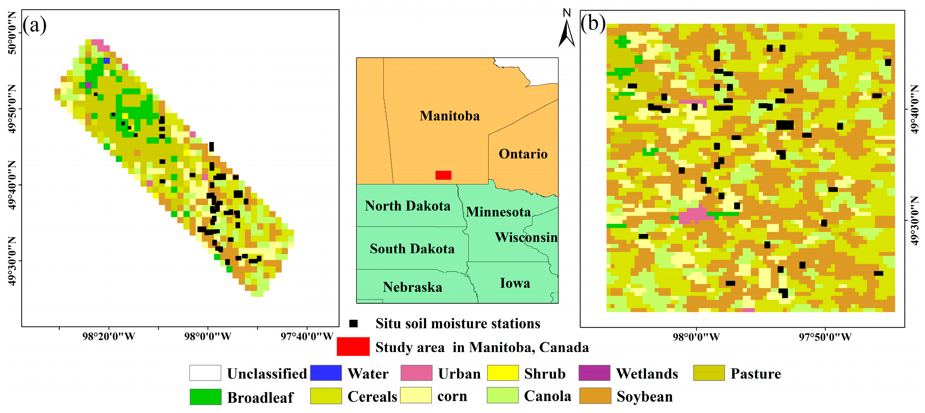
In order to obtain continuously distributed SM in space with a similar spatial resolution to optical SM indexes, we collected the gridded SM obtained from two aircraft field campaigns SMAPVEX12 and SMAPVEX16 in Manitoba, Canada. The two field campaigns belong to the SMAP (Soil Moisture Active Passive, an Earth satellite mission) post-launch calibration and validation activities, which are intended both to assess the quality of the mission products and to support analyses that lead to their improvement. The field campaign was performed every few years such as the Soil Moisture Active Passive Validation Experiment 2012 (SMAPVEX12), 2015 (SMAPVEX15), 2016 Manitoba (SMAPVEX16 Manitoba), 2016 Iowa (SMAPVEX16 Iowa), and 2019–2021 (SMAPVEX19-21). We selected SMAPVEX12 and SMAPVEX16 Manitoba because (1) both of them were located in Manitoba, Canada; (2) they provided gridded SM for free. The SMAPVEX19-21 data are the latest data for this research. However, no gridded SM was provided in SMAPVEX19-21 at the time of this study. More information about the field campaigns comes from the following website:(https://nsidc.org/data/smap/validation/val-data.html (accessed on 17 June 2021).
The airborne field campaigns generally carry the Passive/Active L-band Sensor (PALS), which includes both passive and active L-band sensors that view the land surface at a constant incidence angle of 40° [41,42,43]. The gridded SM retrieved from PALS corresponds to the soil moisture in the top ~5 cm and it was critically validated in the above experiments. It was reported that the SM retrieval performance in non-forested area for SMAPVEX12 is: RMSE (root mean square error) 0.058 m3/m3, bias −0.015 m3/m3, ubRMSE (unbiased RMSE) 0.056 m3/m3, and R (Pearson correlation) 0.87 [44]. The SM uncertainty estimates were reported that the uncertainty of the SM retrieval is within reasonable limits which means that 90% of the data have an uncertainty less than 0.04 m3/m3 [45]. The areas of these field campaigns and their land cover types are presented in Figure 1.

Figure 1.
Spatial distribution and land cover type of (a) SMAPVEX12 and (b) SMAPVEX16-Manitoba.
The SMAPVEX12 campaign covered approximately 6 weeks from 6 June to 7 July in 2012. This campaign is located in an agricultural region in south-central Manitoba, Canada. Each grid cell of the aircraft SM in SMAPVEX12 has a nominal area of approximately 1500 m × 1500 m. The SMAPVEX16 Manitoba experiment spanned more than one month from 8 June to 22 July in 2016. It has the same location as the SMAPVEX12 experiment. The aircraft observed SM from SMAPVEX16 Manitoba has a spatial resolution of 500 m × 500 m. In addition to the aircraft SM, we also collected the in situ observed SM during the field campaigns. The spatial distribution of these stations is also presented in Figure 1.
2.2. Remote Sensing Data
Moderate Resolution Imaging Spectroradiometer (MODIS) surface reflectance products (MOD09A1) and Sentinel-2 multispectral imager (MSI) Level-1C data were utilized in this study. The MOD09A1 data have a spatial resolution of 500 m which can match the spatial resolution of aircraft SM. There are 7 bands of surface reflectance in MOD09A1 which include the Red band (620–670 nm), NIR band (841–875 nm), Blue band (453–479 nm), Green band (545–565 nm), SWIR1 band (1230–1250 nm), SWIR2 band (1628–1652 nm) and SWIR3 band (2105–2155 nm). The HEG (HDF-EOS To GeoTIFF Conversion Tool) was used for preprocessing the original MOD09A1 products. In order to match up aircraft SM in SMAPVEX12, the averaging method was used to aggregate 500 m into 1500 m. The collected Sentinel-2 products are at the level of Level-1C, which is top-of-atmosphere reflectance in cartographic geometry. We used Sen2cor to implement radiation calibration and atmospheric correction to create bottom-of-atmosphere reflectance data. There are 13 spectral bands in MSI data where band 2, 3, 4, and 8 are the Blue, Green, Red, and NIR bands. Band 11 and 12 of MSI are two SWIR bands centered on around 1613.7 nm and 2202.4 nm corresponding to the SWIR2 and SWIR3 of MOD09A1, respectively. For MOD09A1, the aircraft SM were matched with it when their time values intersected. For Sentinel-2 Level-1C, the aircraft SM were matched when their time values were the closest. The metadata information of the study data is presented in Table 1.

Table 1.
Materials used in this study.
3. Methods
3.1. Optical SM Indexes
The 13 typical optical SM indexes were implemented and evaluated in this study, which include PDI, MPDI, DDI, MSI, NDWI, GVMI, LSWI, NMDI, SASI, OPTRAM, VSDI, WISOIL, and SWCI. Table 2 lists the specific algorithms of these SM indexes and their correlation with SM, where the correlation was represented with N to indicate negative correlation and P for positive correlation.
Table 2.
The optical SM indexes used in this study and their correlation with SM.
Where R represents the surface reflectance at various remote sensing bands in MOD09A1. M is the slope of the soil line. fv is the fractional vegetation coverage. Rv,Red and Rv,NIR were 0.05 and 0.5, respectively. OD is the distance from a point in NIR and Red space to the origin point. is the angle formed at vertex SWIR1 by the NIR-SWIR1-SWIR2 reflectance bands. STR is the SWIR Transformed Reflectance, . OPTRAM is derived from the STR and NDVI space. When NDVI is 0, the value of dry side is id, and the value of wet side is . and are the slopes of dry side and wet side, respectively. N stands for negative correlation. P stands for positive correlation.
3.2. Evaluation Methods
The evaluation was conducted three-fold. Firstly, MODIS-derived SM indexes were compared with continuously distributed aircraft SM from SMAPVEX12 and SMAPVEX16. Secondly, they were also evaluated with the in situ observed SM during the two aircraft experiments. Thirdly, Sentinel-2 MSI-derived SM indexes were compared with the aircraft SM from SMAPVEX16. Since the optical SM index provides an indicator of the SM rather than the absolute value of SM, Pearson’s correlation coefficient (R) between the optical SM index and the aircraft or in situ SM was used as a measurement. The higher absolute value of R indicates better consistence and as a result demonstrates better performance. Box chart statistics of R were used to represent the performance at the statistical level. Additionally, a linear equation was used to fit optical SM indexes and aircraft or in situ SM which can be expressed as:
where θ represents the aircraft or in situ SM; SMI is the optical SM index; a and b are coefficients. Several measurements were employed to measure the performance of SMI in fitting aircraft or in situ SM, which include the coefficient of determination (R2), Root Mean Square Error (RMSE), normalized RMSE (nRMSE), Mean Absolute Error (MAE), and F-value test for comparative analysis (F). Mathematically, higher R2 and F with smaller RMSE/nRMSE and MAE represent better modeling accuracy and better performance of the SMI. The following equations were used to calculate R2, RMSE, nRMSE, MAE, and F:
where and are measured SM and its average; and are estimated SM and its average; and are the measured maximum and minimum SM; n is the sample number.
4. Results
4.1. Comparing MODIS-Derived SM Indexes with Aircraft SM
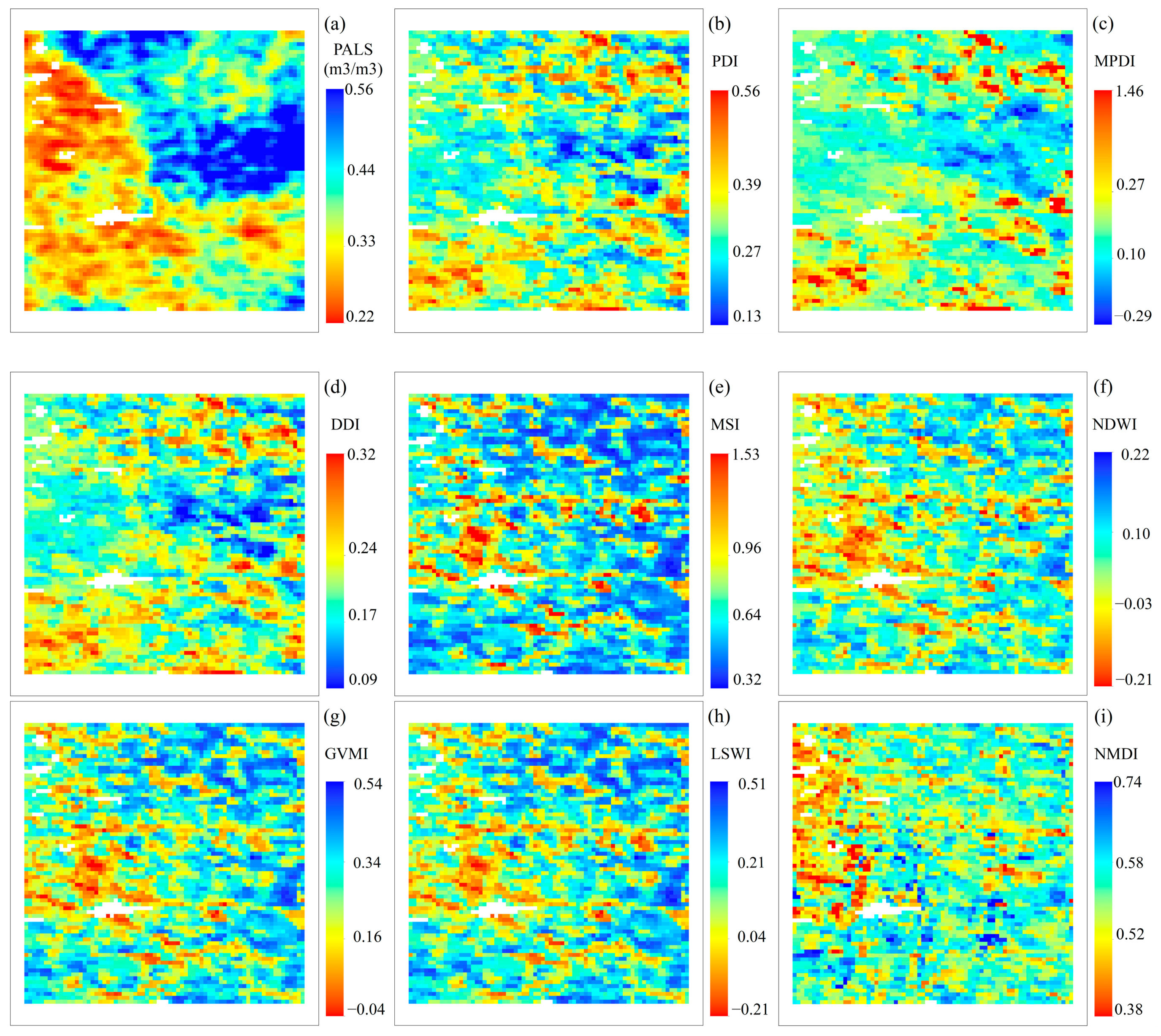
Figure 2 presents the spatial distribution of the aircraft SM and the optical SM indexes on 19 June 2016 during the SMAPVEX16 Manitoba experiment. Figure 2a is the aircraft SM which indicates that there are some low-value areas of SM in the lower left part and some high-value areas in the upper right part of the study area. Figure 2b–l are the spatial distribution of SM indexes PDI, MPDI, DDI, MSI, NDWI, GVMI, LSWI, NMDI, SASI, WISOIL and SWCI, respectively. Figure 2m shows the OPTRAM model and Figure 2n shows the VSDI index. We have adjusted the color table in all subfigures to unify the indication of SM variation. It can be clearly seen that the OPTRAM and VSDI index achieved the best performance in presenting the spatial variation of SM compared with the aircraft SM. The other indexes presented worse performance than OPTRAM and VSDI in indicating the spatial variation of SM.
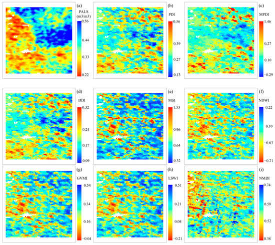
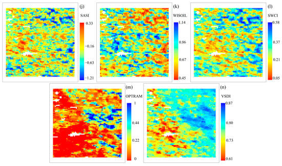
Figure 2.
Spatial distribution of the aircraft SM and optical SM indexes during the SMAPVEX16 Manitoba experiment on 19 June 2016 where (a) is the aircraft SM and (b–n) are the thirteen optical SM indexes.
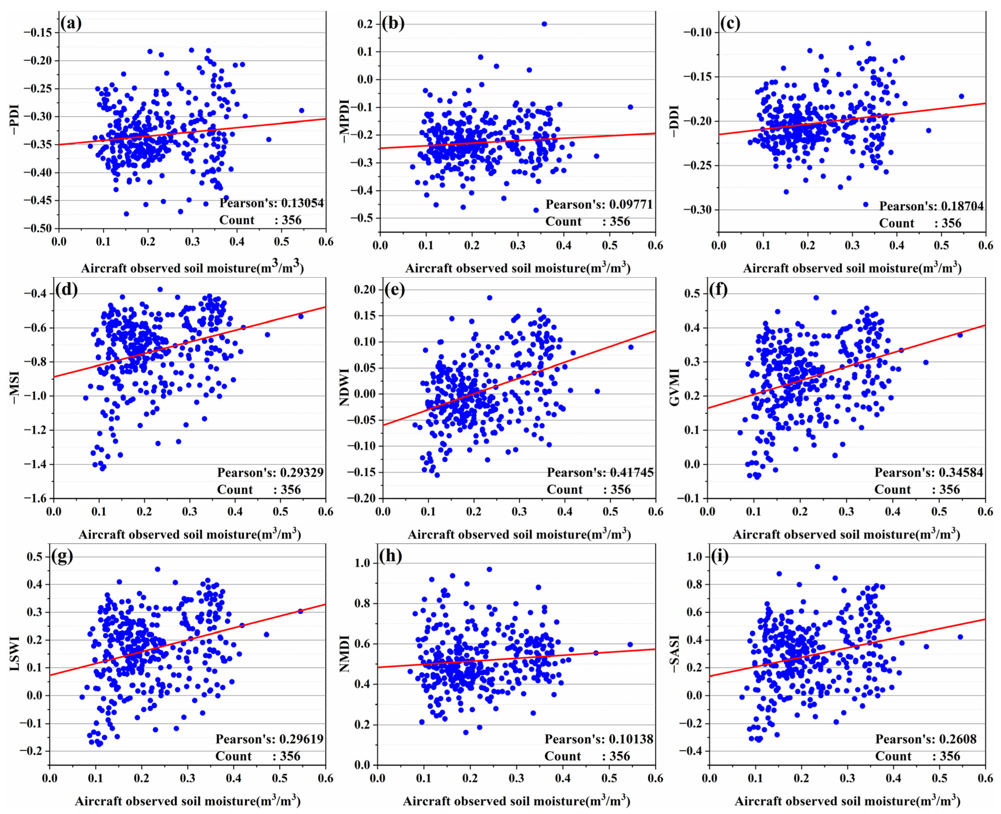
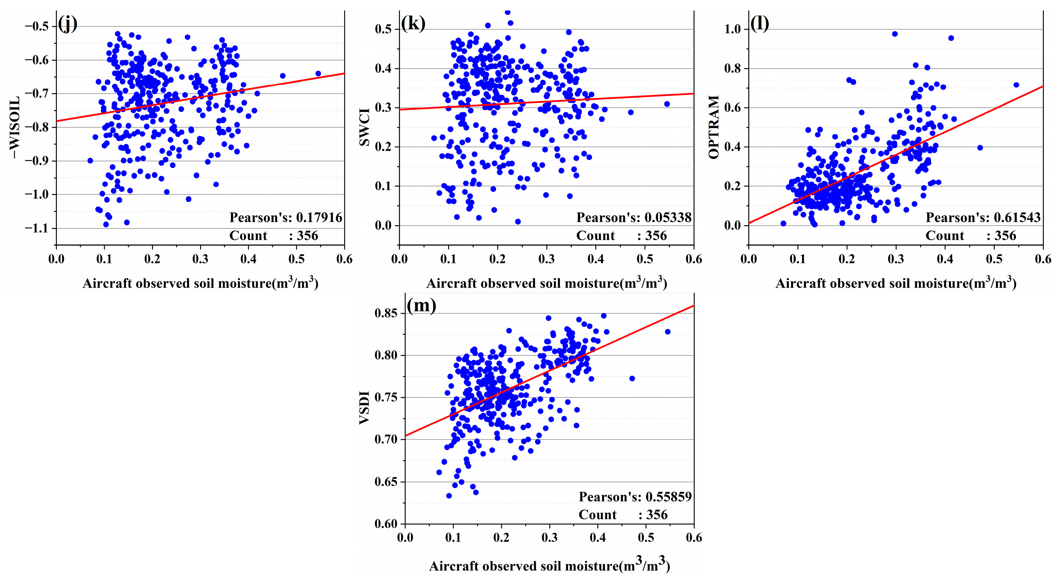
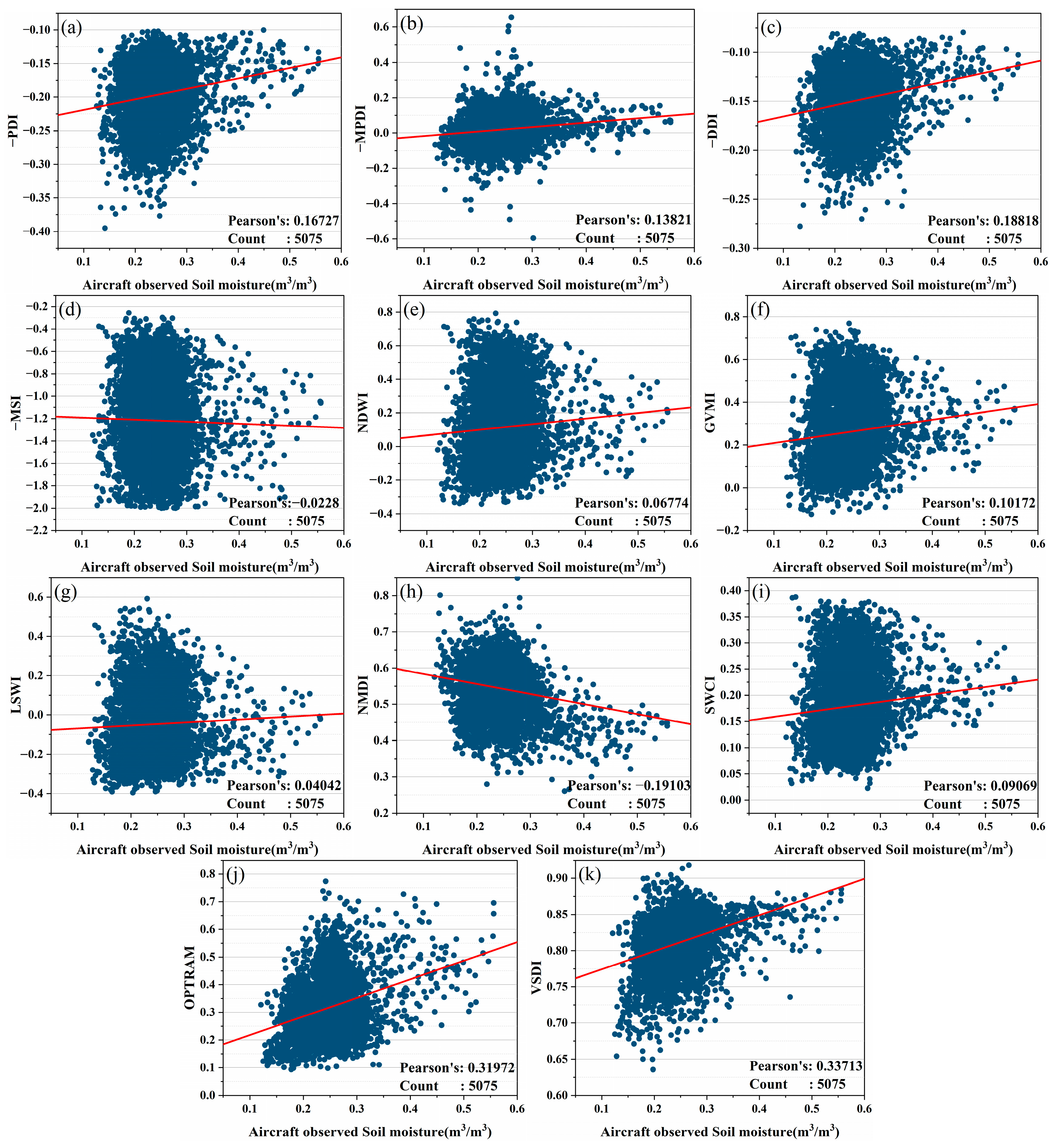
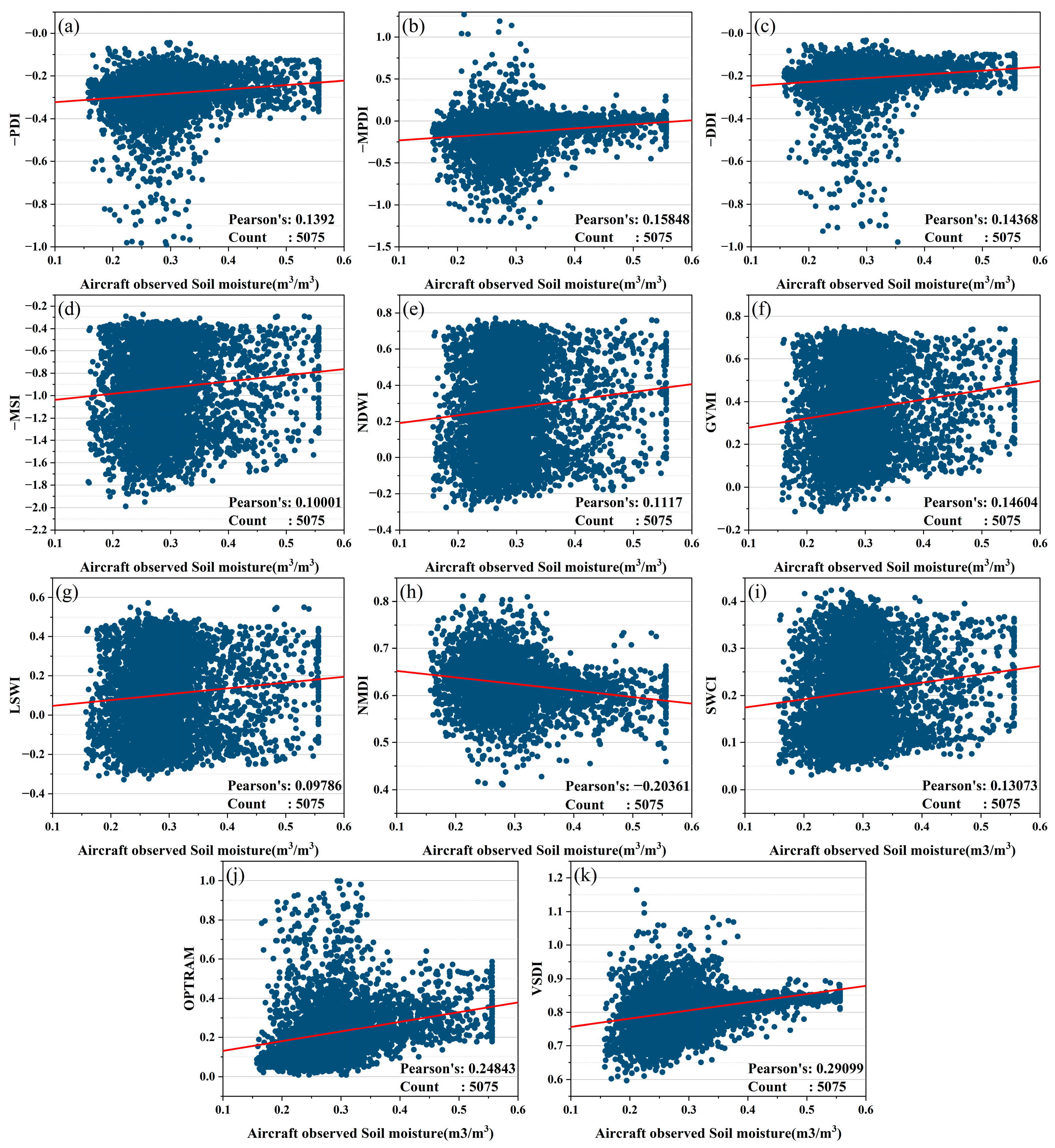
In another evaluation, scatter plots between the aircraft SM and optical SM index were presented. As shown in Figure 3, the comparisons were conducted on 15 June 2012 during the SMAPVEX12 experiment. The optical SM index with negative correlation with SM is expressed as a negative value in Figure 3. Similar to the results in Figure 2, we found that OPTRAM achieved the highest R at the value of 0.61 and the VSDI index achieved an R of 0.56. The other indexes had smaller R values.
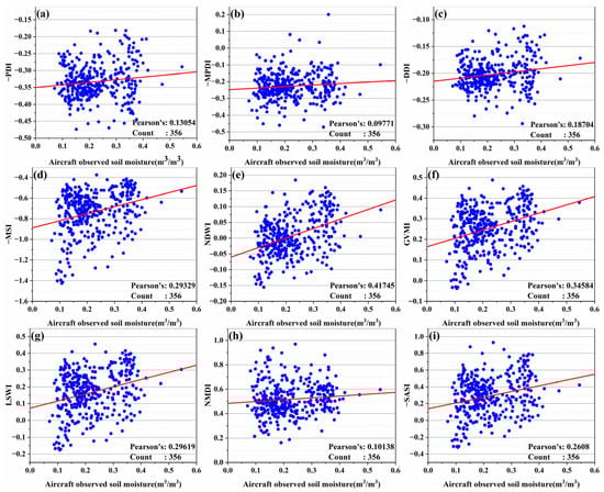

Figure 3.
Scatter plots between the aircraft SM and the optical SM indexes during the SMAPVEX12 on 15 June 2012 where (a) PDI, (b) MPDI, (c) DDI, (d) MSI, (e) NDWI, (f) GVMI, (g) LSWI, (h) NMDI, (i) SASI, (j) WISOIL, (k) SWCI, (l) OPTRAM, and (m) VSDI.
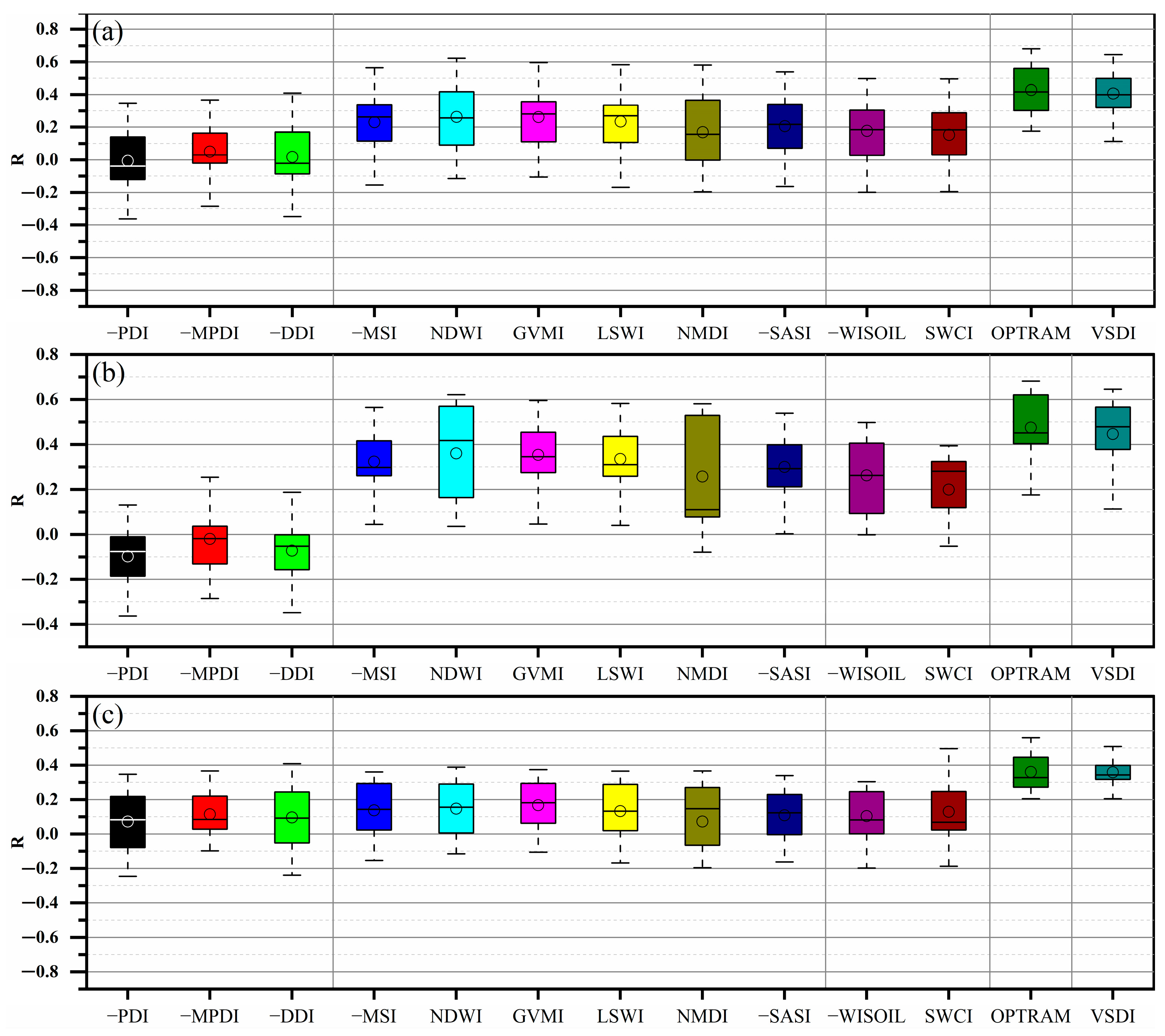
In order to evaluate the results comprehensively, we constructed box plot statistics on the R values between the aircraft SM and the optical SM indexes, which are illustrated in Figure 4. The statistics were constructed on the whole study period of all aircraft experiments (Figure 4a) and each aircraft experiment (Figure 4b,c). The optical SM index with negative correlation with SM is also expressed as a negative value. During the SMAPVEX12, the R values of OPTRAM ranged from 0.4 to 0.6 and the R of VSDI varied between 0.38 and 0.58. The PDI, MPDI, and DDI achieved the worst performance since their R values varied from −0.2 to 0.1. The other indexes achieved a performance better than the PDI, MPDI, and DDI but worse than the OPTRAM and VSDI. The same phenomenon was found during the SMAPVEX16 Manitoba.
Figure 4.
Box plots of Pearson’s R between the aircraft SM and the optical SM indexes during the whole study period in (a) all experiments, (b) the SMAPVEX12 experiment, (c) the SMAPVEX16 Manitoba experiment.
Table 3 lists the average R2, RMSE, nRMSE, MAE, and F values of each SMI as compared with the aircraft SM. As can be seen from the table, the R2 and F of the OPTRAM index is the largest followed by the VSDI index and the smallest R2 and F values were found for the DDI, PDI, and MPDI indexes. Similarly, the OPTRAM and VSDI achieved the lowest values for RMSE, nRMSE, and MAE. They are 7.01%, 16.37%, and 5.53% for the OPTRAM and 7.13%, 16.65%, and 5.65% for the VSDI, respectively. In summary, the comparisons with aircraft SM indicated that the OPTRAM and VSDI achieved the best performance statistically. The PDI, MPDI, and DDI achieved the worst performance and the performances achieved by the other SM indexes varied between them.
Table 3.
Comparisons between aircraft SM and optical SMIs with MODIS data.
4.2. Evaluating MODIS-Derived SM Indexes with In Situ Observed SM
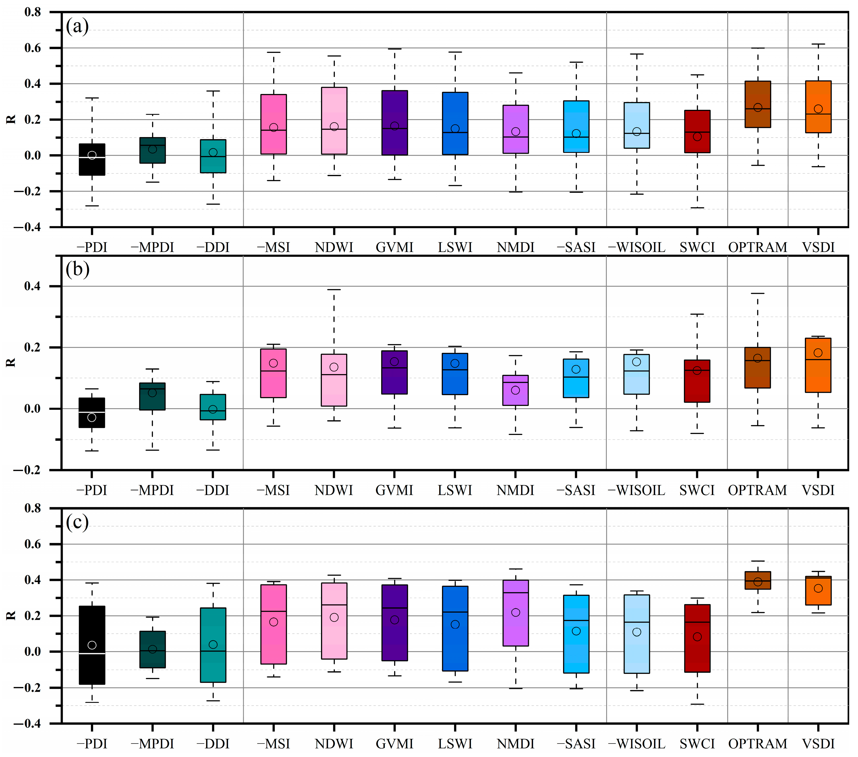
Figure 5 presents the evaluation results with in situ observed SM, where subfigure (a) is the result for all experiments, (b) is for the SMAPVEX12 experiment, and (c) is for the SMAPVEX16 experiment. As shown in Figure 5a, the OPTRAM model and VSDI index had the highest R value with in situ measured SM. The other indexes had lower R values and the worst performance was found for the DDI, PDI, and MPDI indexes. The same phenomenon was also found for Figure 5b,c.
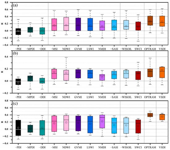
Figure 5.
Box plots of Pearson’s R between the in situ observed SM and the optical SM indexes during the whole study period in (a) all experiments, (b) SMAPVEX12 experiment, and (c) SMAPVEX16 Manitoba experiment.
Table 4 lists the average R2, RMSE, nRMSE, MAE, and F values of each SMI as compared with the in situ SM. Again, the OPTRAM and VSDI achieved the biggest R2 and F values and the lowest RMSE, nRMSE, and MAE values. They achieved the best performance. The PDI, MPDI, and DDI still achieved the worst performance and the performance achieved by the other SM indexes varied between them.
Table 4.
Comparisons between in situ SM and optical SMIs with MODIS data.
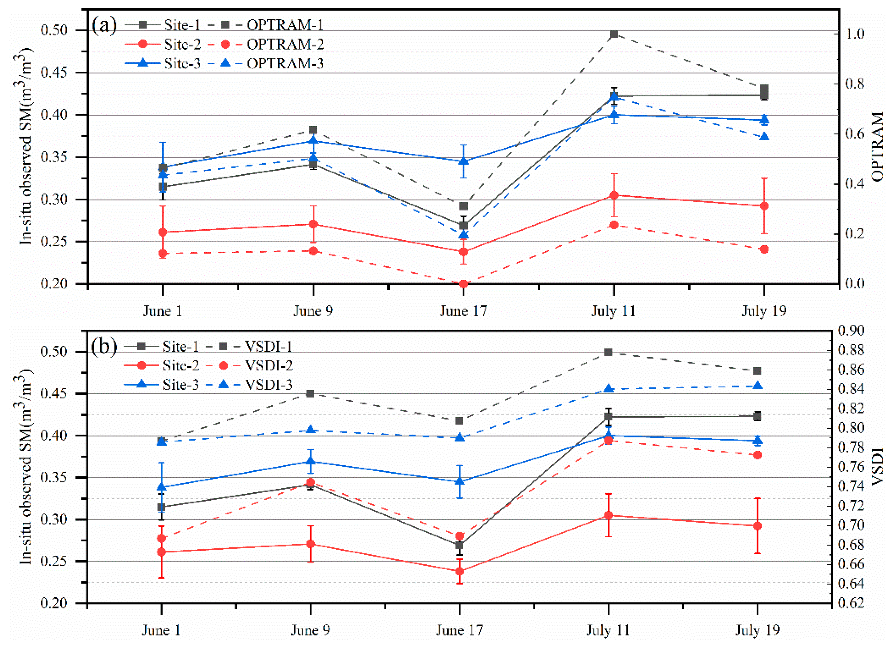
The above evaluations demonstrate that the OPTRAM model and VSDI index achieved the best performance among the various optical SM indexes. They were subsequently selected to conduct a temporal variation analysis. Taking three stations for example, Figure 6 presents the temporal variation of the in situ observed SM and OPTRAM/VSDI index. A fluctuating variation of in situ observed SM can be found in Figure 6. Furthermore, the temporal variations of OPTRAM and VSDI indexes were found to be consistent with that of in situ observed SM. The results in Figure 6 demonstrate the validity of OPTRAM and VSDI indexes in depicting the temporal variation of SM.
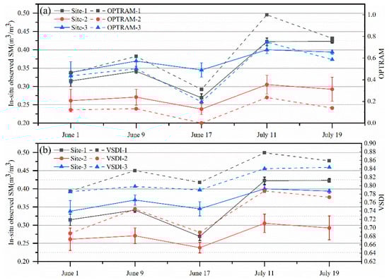
Figure 6.
Temporal variation of the in situ observed SM, (a) OPTRAM and (b) VSDI indexes at three sites during the SMAPVEX16_Manitoba experiment, where the site ID of Sites 1, 2, and 3 are 31, 210, and 221, respectively.
4.3. Comparing Sentinel MSI-Derived SM Indexes with Aircraft SM
For further evaluation, the optical SM indexes calculated by Sentinel-2 MSI data were compared with aircraft SM. The optical SM indexes that can be calculated with Sentinel-2 MSI data are PDI, MPDI, DDI, MSI, NDWI, GVMI, LSWI, NMDI, OPTRAM, VSDI, and SWCI. Figure 7 and Figure 8 show the scatter plot between the optical SM index and aircraft SM on 11 June and 20 June 2016. There is only one day difference between the Sentinel-2 MSI imaging date and aircraft SM date. As shown in Figure 7, the R value between VSDI index and aircraft SM data around 0.34, and that of the OPTRAM index is around 0.32. The other indexes had R values less than that of VSDI and OPTRAM. In Figure 8, the R value of the VSDI index is 0.29 and that of the OPTRAM is 0.25. Again, they achieved the best performance among the various optical SM indexes.

Figure 7.
(a–k) Scatter plot between the aircraft SM and Sentinel MSI-derived SM indexes on 11 June 2016 during the SMAPVEX16 Manitoba experiment.
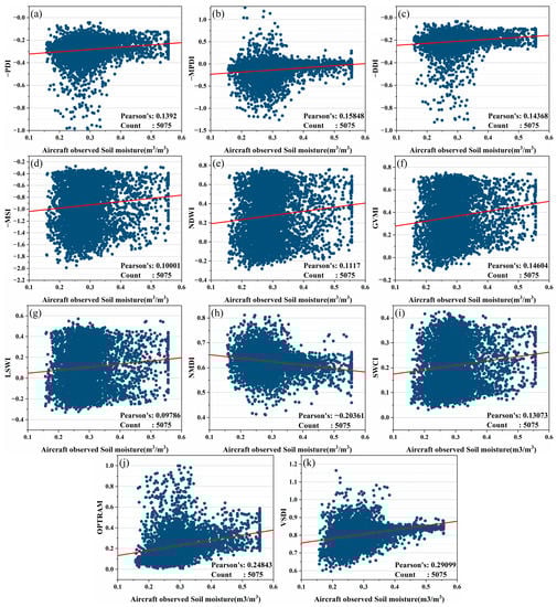
Figure 8.
(a–k) Scatter plot between aircraft SM and Sentinel MSI-derived SM indexes on 20 June 2016 during the SMAPVEX16 Manitoba experiment.
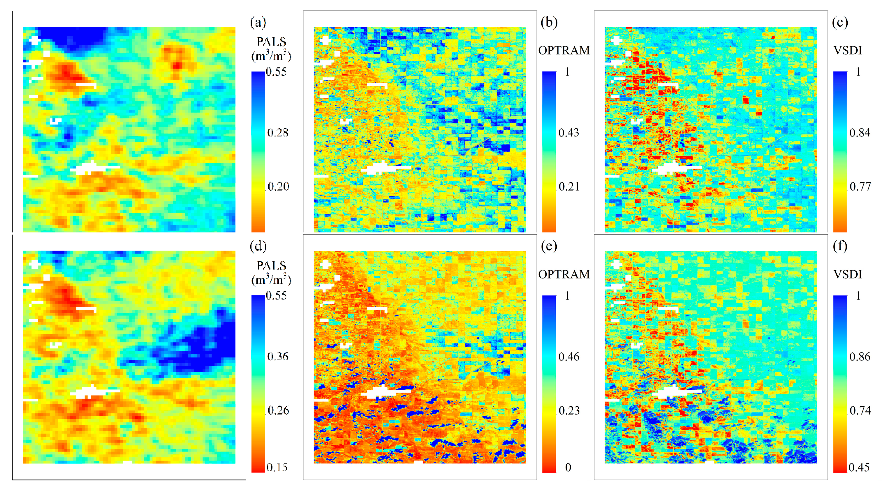
As regards the VSDI and OPTRAM, we think they are comparable with each other. That is because (1) during the evaluation of MODIS-derived SM indexes, the OPTRAM was a little better than the VSDI; (2) during the evaluation of Sentinel MSI-derived SM indexes, the VSDI was a little better than the OPTRAM. Moreover, Figure 9 shows the spatial distribution of the aircraft SM, OPTRAM and VSDI on 11 June and 20 June 2016. Sentinel-2 MSI data have higher spatial resolution and thus show more detailed spatial distribution. As shown in Figure 9, aircraft SM, OPTRAM and VSDI have similar spatial distribution.
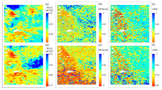
Figure 9.
Spatial distribution of the aircraft SM, the OPTRAM and VSDI indexes on 11 June (a–c) and on 20 June (d–f), 2016 during the SMAPVEX16-Manitoba experiment.
5. Discussion
5.1. Implications
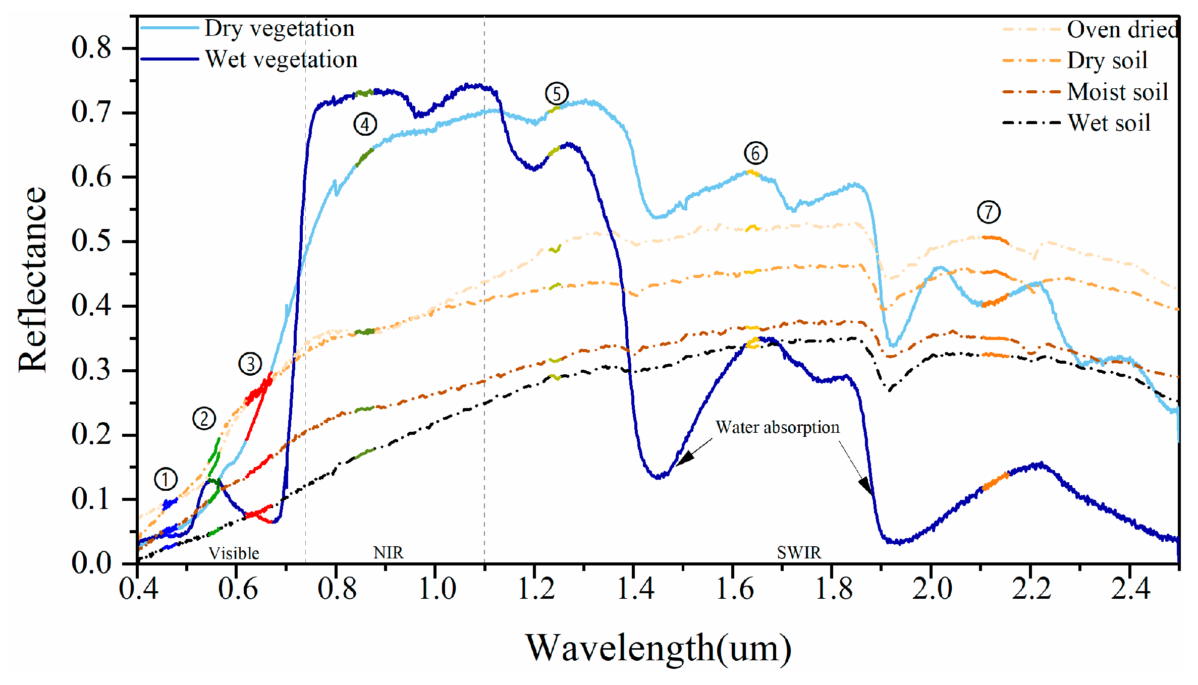
The above results indicate that VSDI and OPTRAM have comparable performance, and they outperform the other optical SM indexes. We think that this phenomenon can be interpreted by the spectrum features of soil and vegetation. Figure 10 presents the spectrum features of vegetation and soil with differing water content. The spectral reflectance curves were obtained from the spectral libraries provided by ENVI software.

Figure 10.
Spectrum features of vegetation and soil with different water content where ①–⑦ represent the band positions of Blue, Green, Red, NIR, SWIR1, SWIR2, and SWIR3 in MOD09A1.
We can find that, when vegetation suffers water stress, absorption in blue and red bands decreases, and changes in the red spectrum are more sensitive than those in the blue spectrum. The reflectance of NIR is mainly sensitive to changes in the internal structure of leaves which show a smaller response to changes in water content. In contrast, the reflectance of SWIR bands increased significantly when leaves were deficient in water. Regarding the spectral response to soil moisture changes, we found that the whole spectral reflectance of soil decreases with the increase in soil moisture content. The variation range of soil reflectance with the change in soil moisture is relatively small in the region of the visible light spectrum, but relatively great in a longer wavelength region. As a result, SWIR and Red bands are relatively sensitive bands to the change in soil and vegetation moisture, while the NIR and Blue bands are relatively insensitive bands to soil and vegetation moisture change.
Based on the above recognition, the optical SM indexes can be classified into the following five categories. Table 5 shows the classification of typical optical soil moisture indices. This classification is based on varied combinations of remote sensing bands. PDI, MPDI, and DDI can be organized into one category, since they use the Red band as the measurement or sensitive band and NIR as the reference or the insensitive band. The second category includes MSI, NDWI, GVMI, LSWI, NMDI, and SASI because they employ SWIR bands as the measurement band and NIR as the reference band. WISOIL and SWCI are recognized as one category since they only used SWIR bands. For OPTRAM and VSDI, the Red band and SWIR band were combined as measurement band which is different from the other indexes. There are two sensitive bands used in OPTRAM and VSDI, while there is usually only one sensitive band used in the other optical SM indexes, which may be the main reason why they achieved the best performance in the above evaluations. However, we think OPTRAM and VSDI should be organized into different categories because different reference bands were used in them, i.e., NIR for OPTRAM and Blue for VSDI.
Table 5.
Classification of the typical optical SM indexes.
5.2. Improvements
Firstly, we would like to improve the VSDI index since that (1) it achieved very good performance in the above evaluations, and (2) its mathematical expression is very simple which may not highlight the difference between sensitive and insensitive bands of soil and vegetation moisture. Consequently, the following expressions were created which can be labeled Modified VSDI 1 (MVSDI1), MVSDI2, MVSDI3, MVSDI4, and MVSDI5.
where , , , and are spectral reflectance at the corresponding bands of MOD09A1, respectively.
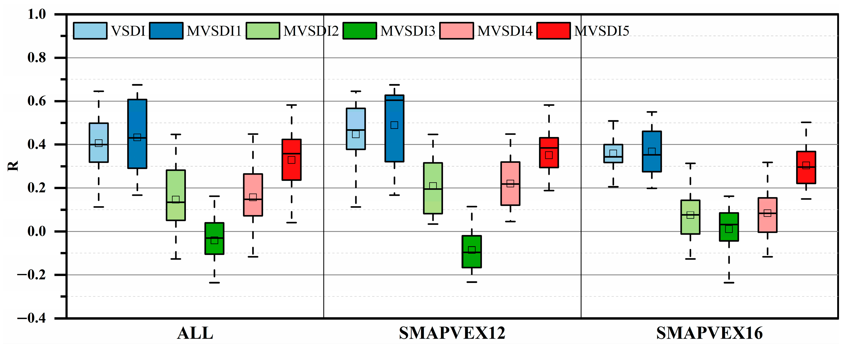
Figure 11 presents the comparisons between VSDI, modified VSDIs, and aircraft SM. An interesting phenomenon can be found in Figure 11 that the varied modifications in mathematical expression of VSDI do not improve the performance of VSDI. Specifically, MVSDI2, MVSDI3, MVSDI4, and MVSDI5 did not outperform the VSDI and MVSDI1 in the evaluations with SMAPVEX12 data, SMAPVEX16 data, and All experiments data. In contrast, MVSDI1 achieved better performance than the VSDI in the above evaluations. Notice that MVSDI1 and VSDI have the same mathematical expression while the former adds a sensitive band, i.e., SWIR1.

Figure 11.
Comparisons between VSDI, modified VSDIs, and aircraft SM.
Furthermore, we tried to improve the OPTRAM because the blue band, a robust reference or insensitive band for soil and vegetation moisture, is not integrated into it. As we know, OPTRAM is derived from the STR and NDVI space, which is a derivative of the Land surface temperature (LST) and NDVI space. Their basic theory is to strip the interference of vegetation on the SM’s indicator, STR or LST. In view of this basic theory, we constructed two new indexes by creating VSDI and NDVI space, as well as creating MVSDI1 and NDVI space. Based on the two new spaces and referring to the calculation of OPTRAM, the two new indexes can be obtained. Temporarily, we labeled them NDVI-VSDI and NDVI-MVSDI1.
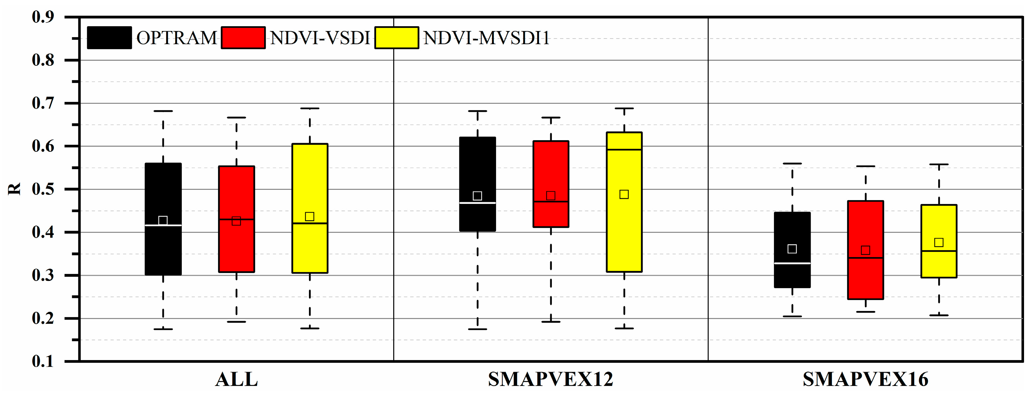
Figure 12 presents the comparisons between OPTRAM, modifications of OPTRAM (i.e., NDVI-VSDI and NDVI-MVSDI1), and the aircraft SM. We found that the NDVI-VSDI is only slightly better than the OPTRAM, as compared with the aircraft SM. However, NDVI-MVSDI1 achieved a significantly better performance than the OPTRAM for all experiments.

Figure 12.
Comparisons between OPTRAM, modifications of OPTRAM (i.e., NDVI-VSDI and NDVI-MVSDI1), and aircraft SM.
6. Conclusions
In this study, 13 optical SM indexes that were constructed with the spectral reflectance around 0.4~2.0 μm were compared with aircraft and in situ SM observations from two airborne field campaigns, SMAPVEX12 and SMAPVEX16 in Manitoba, Canada. The results can be summarized as follows:
- (1)
- The VSDI and OPTRAM indexes achieved the best performance among the thirteen optical SM indexes as compared with aircraft and in situ observed SM. They also presented results consistent in temporal variation with the in situ observed SM.
- (2)
- The VSDI and OPTRAM presented comparable performance with each other; while the former has very simple calculation and expression, the latter requires a complex process to determine the dry and wet boundaries.
- (3)
- The VSDI and OPTRAM indexes both capitalize on two bands (i.e., the Red and SWIR bands) of the soil and vegetation spectrum sensitive to water content, whereas the other eleven SM indexes only employ one sensitive band (i.e., Red or SWIR band). This may be the main reason for the evaluation results. A classification of the optical SM indexes was proposed according to the combination of the sensitive band and insensitive band.
- (4)
- Based on the classification, improvements to the VSDI and OPTRAM were proposed and validated in this study, by adding a more sensitive band to the VSDI and combining the NDVI and modified VSDI into a new feature space for calculating optical SM indexes such as OPTRAM.
The optical SM indexes have the features of convenience, efficiency and high spatial resolution, which are of great significance to monitoring agricultural drought, soil moisture, as well as the ecological environment. This study provides a reference to select and utilize the current numerous optical SM indexes. The improvements attempted in this study open avenues for further optimization of optical SM indexes. It is worth noting that the studied optical SM indexes were designed for soil and vegetation areas. They may not work for the areas with bare rock, built-up areas, areas with snow or ice, etc.
Author Contributions
Conceptualization, H.S.; methodology, H.S.; formal analysis, H.S., H.L. and Y.M.; writing—original draft preparation, H.S., H.L. and Y.M.; resources, H.L. and Q.X.; data curation, H.L. and Q.X.; writing—review and editing, H.S., H.L. and Y.M. All authors have read and agreed to the published version of the manuscript.
Funding
This research was funded by the National Natural Science Foundation of China, grant number 41871338; Yue Qi Young Scholar Project, CUMTB2018; and Fundamental Research Funds for the Central Universities, grant number 2020YJSDC08.
Institutional Review Board Statement
Not appliable.
Informed Consent Statement
Not appliable.
Data Availability Statement
Not applicable.
Acknowledgments
The authors would like to thank the European Space Agency for providing the Sentinel-2 data. Thanks are also expressed to NASA Distributed Active Archive Center at NSIDC and NASA Land Processes Distributed Active Archive Center for providing the SMAPVEX12, SMAPVEX16, and MODIS data.
Conflicts of Interest
The authors declare no conflict of interest.
References
- Seneviratne, S.I.; Corti, T.; Davin, E.L.; Hirschi, M.; Jaeger, E.B.; Lehner, I.; Orlowsky, B.; Teuling, A.J. Investigating soil moisture-climate interactions in a changing climate: A review. Earth-Sci. Rev. 2010, 99, 125–161. [Google Scholar] [CrossRef]
- World Meteorological Organization. Essential Climate Variables. Available online: https://public.wmo.int/en/programmes/global-climate-observing-system/essential-climate-variables (accessed on 17 May 2021).
- Petropoulos, G.P.; Ireland, G.; Barrett, B. Surface soil moisture retrievals from remote sensing: Current status, products & future trends. Phys. Chem. Earth 2015, 83–84, 36–56. [Google Scholar] [CrossRef]
- Dobriyal, P.; Qureshi, A.; Badola, R.; Hussain, S.A. A review of the methods available for estimating soil moisture and its implications for water resource management. J. Hydrol. 2012, 458, 110–117. [Google Scholar] [CrossRef]
- AghaKouchak, A.; Farahmand, A.; Melton, F.S.; Teixeira, J.; Anderson, M.C.; Wardlow, B.D.; Hain, C.R. Remote sensing of drought: Progress, challenges and opportunities. Rev. Geophys. 2015, 53, 452–480. [Google Scholar] [CrossRef] [Green Version]
- Sun, H.; Chen, Y.; Sun, H. Comparisons and classification system of typical remote sensing indexes for agricultural drought. Trans. Chin. Soc. Agric. Eng. 2012, 28, 147–154. [Google Scholar]
- Sun, H.; Zhao, X.; Chen, Y.; Gong, A.; Yang, J. A new agricultural drought monitoring index combining MODIS NDWI and day-night land surface temperatures: A case study in China. Int. J. Remote Sens. 2013, 34, 8986–9001. [Google Scholar] [CrossRef]
- Robinson, D.A.; Campbell, C.S.; Hopmans, J.W.; Hornbuckle, B.K.; Jones, S.B.; Knight, R.; Ogden, F.; Selker, J.; Wendroth, O. Soil moisture measurement for ecological and hydrological watershed-scale observatories: A review. Vadose Zone J. 2008, 7, 358–389. [Google Scholar] [CrossRef] [Green Version]
- Dai, A.; Trenberth, K.E.; Qian, T.T. A global dataset of Palmer Drought Severity Index for 1870–2002: Relationship with soil moisture and effects of surface warming. J. Hydrometeorol. 2004, 5, 1117–1130. [Google Scholar] [CrossRef]
- Anderson, M.C.; Norman, J.M.; Mecikalski, J.R.; Otkin, J.A.; Kustas, W.P. A climatological study of evapotranspiration and moisture stress across the continental United States based on thermal remote sensing: 2. Surface moisture climatology. J. Geophys. Res.-Atmos. 2007, 112, D11112. [Google Scholar] [CrossRef]
- Sun, H.; Zhou, B.; Zhang, C.; Liu, H.; Yang, B. DSCALE_mod16: A Model for Disaggregating Microwave Satellite Soil Moisture with Land Surface Evapotranspiration Products and Gridded Meteorological Data. Remote Sens. 2020, 12, 980. [Google Scholar] [CrossRef] [Green Version]
- Babaeian, E.; Sadeghi, M.; Jones, S.B.; Montzka, C.; Vereecken, H.; Tuller, M. Ground, Proximal, and Satellite Remote Sensing of Soil Moisture. Rev. Geophys. 2019, 57, 530–616. [Google Scholar] [CrossRef] [Green Version]
- Sun, H.; Cai, C.; Liu, H.; Yang, B. Microwave and Meteorological Fusion: A method of Spatial Downscaling of Remotely Sensed Soil Moisture. IEEE J. Sel. Top. Appl. Earth Observ. Remote Sens. 2019, 12, 1107–1119. [Google Scholar] [CrossRef]
- Peng, J.; Loew, A.; Merlin, O.; Verhoest, N.E.C. A review of spatial downscaling of satellite remotely sensed soil moisture. Rev. Geophys. 2017, 55, 341–366. [Google Scholar] [CrossRef]
- Das, N.N.; Entekhabi, D.; Njoku, E.G. An Algorithm for Merging SMAP Radiometer and Radar Data for High-Resolution Soil-Moisture Retrieval. IEEE Trans. Geosci. Remote Sens. 2011, 49, 1504–1512. [Google Scholar] [CrossRef]
- Sun, H.; Cui, Y. Evaluating Downscaling Factors of Microwave Satellite Soil Moisture Based on Machine Learning Method. Remote Sens. 2021, 13, 133. [Google Scholar] [CrossRef]
- Sun, H.; Zhou, B.; Li, H.; Ruan, L. A primary study on downscaling microwave soil moisture with MOD16 and SMAP. Yaogan Xuebao J. Remote Sens. 2021, 25, 776–790. [Google Scholar] [CrossRef]
- Sun, H.; Liu, W.; Wang, Y.; Yuan, S. Evaluation of Typical Spectral Vegetation Indices for Drought Monitoring in Cropland of the North China Plain. IEEE J. Sel. Top. Appl. Earth Observ. Remote Sens. 2017, 10, 5404–5411. [Google Scholar] [CrossRef]
- Ishida, T.; Ando, H.; Fukuhara, M. Estimation of complex refractive index of soil particles and its dependence on soil chemical properties. Remote Sens. Environ. 1991, 38, 173–182. [Google Scholar] [CrossRef]
- Zhang, D.J.; Zhou, G.Q. Estimation of Soil Moisture from Optical and Thermal Remote Sensing: A Review. Sensors 2016, 16, 1308. [Google Scholar] [CrossRef] [Green Version]
- Petropoulos, G.P.; Srivastava, P.K.; Ferentinos, K.P.; Hristopoulos, D. Evaluating the capabilities of optical/TIR imaging sensing systems for quantifying soil water content. Geocarto Int. 2018, 35, 494–511. [Google Scholar] [CrossRef]
- Bowers, S.A.; Smith, S.J. Spectrophotometric Determination of Soil Water Content. Soil Sci. Soc. Am. J. 1972, 36, 978–980. [Google Scholar] [CrossRef]
- Liu, W.D.; Baret, F.; Gu, X.F.; Tong, Q.X.; Zheng, L.F.; Zhang, B. Relating soil surface moisture to reflectance. Remote Sens. Environ. 2002, 81, 238–246. [Google Scholar]
- Lobell, D.B.; Asner, G.P. Moisture effects on soil reflectance. Soil Sci. Soc. Am. J. 2002, 66, 722–727. [Google Scholar] [CrossRef]
- Jacquemoud, S.; Baret, F.; Hanocq, J.F. Modeling spectral and bidirectional soil reflectance. Remote Sens. Environ. 1992, 41, 123–132. [Google Scholar] [CrossRef]
- Zhang, N.; Hong, Y.; Qin, Q.M.; Liu, L. VSDI: A visible and shortwave infrared drought index for monitoring soil and vegetation moisture based on optical remote sensing. Int. J. Remote Sens. 2013, 34, 4585–4609. [Google Scholar] [CrossRef]
- Ghulam, A.; Qin, Q.; Zhan, Z. Designing of the perpendicular drought index. Environ. Geol. 2006, 52, 1045–1052. [Google Scholar] [CrossRef]
- Ghulam, A.; Qin, Q.M.; Teyip, T.; Li, Z.L. Modified perpendicular drought index (MPDI): A real-time drought monitoring method. ISPRS-J. Photogramm. Remote Sens. 2007, 62, 150–164. [Google Scholar] [CrossRef]
- Yang, N.; Qin, Q.; Jin, C.; Yao, Y. The comparison and application of the methods for monitoring farmland drought based on nir-red spectral space. In Proceedings of the 2008 IEEE International Geoscience and Remote Sensing Symposium—Proceedings, Boston, MA, USA, 6–11 July 2008; pp. 871–874. [Google Scholar]
- Bryant, R.; Thoma, D.; Moran, S.; Goodrich, D.; Keefer, T.; Paige, G.; Skirvin, S. Evaluation of hyperspectral, infrared temperature and radar measurements for monitoring surface soil moisture. In Proceedings of the First Interagency Conference on Research in the Watersheds, Benson, AZ, USA, 27–30 October 2003. [Google Scholar]
- Gao, B.-c. NDWI—A normalized difference water index for remote sensing of vegetation liquid water from space. Remote Sens. Environ. 1996, 58, 257–266. [Google Scholar] [CrossRef]
- Ceccato, P.; Gobron, N.; Flasse, S.; Pinty, B.; Tarantola, S. Designing a spectral index to estimate vegetation water content from remote sensing data: Part 2. Validation and applications. Remote Sens. Environ. 2002, 82, 198–207. [Google Scholar] [CrossRef]
- Xiao, X.; Zhang, Q.; Braswell, B.; Urbanski, S.; Boles, S.; Wofsy, S.; Moore, B., III; Ojima, D. Modeling gross primary production of temperate deciduous broadleaf forest using satellite images and climate data. Remote Sens. Environ. 2004, 91, 256–270. [Google Scholar] [CrossRef]
- Wang, L.L.; Qu, J.J. NMDI: A normalized multi-band drought index for monitoring soil and vegetation moisture with satellite remote sensing. Geophys. Res. Lett. 2007, 34, 5. [Google Scholar] [CrossRef]
- Khanna, S.; Palacios-Orueta, A.; Whiting, M.L.; Ustin, S.L.; Riano, D.; Litago, J. Development of angle indexes for soil moisture estimation, dry matter detection and land-cover discrimination. Remote Sens. Environ. 2007, 109, 154–165. [Google Scholar] [CrossRef]
- Sadeghi, M.; Babaeian, E.; Tuller, M.; Jones, S.B. The optical trapezoid model: A novel approach to remote sensing of soil moisture applied to Sentinel-2 and Landsat-8 observations. Remote Sens. Environ. 2017, 198, 52–68. [Google Scholar] [CrossRef] [Green Version]
- Du, X.; Wang, S.; Zhou, Y.; Wei, H. Construction and Verification of a New Land Surface Water Content Model Based on MODIS Data; Geomatics and Information Science of Wuhan University: Wuhan, China, 2007; pp. 205–207+211. (In Chinese) [Google Scholar]
- Yue, J.; Tian, J.; Tian, Q.; Xu, K.; Xu, N. Development of soil moisture indices from differences in water absorption between shortwave-infrared bands. ISPRS J. Photogramm. Remote Sens. 2019, 154, 216–230. [Google Scholar] [CrossRef]
- Kubiak, K.; Justyna, S.; Jakub, S.; Spiralski, M. Estimation of Bare Soil Moisture from Remote Sensing Indices in the 0.4–2.5 mm Spectral Range. Trans. Aerosp. Res. 2021, 2021, 1–11. [Google Scholar] [CrossRef]
- Sun, H.; Xu, Q. Evaluating Machine Learning and Geostatistical Methods for Spatial Gap-Filling of Monthly ESA CCI Soil Moisture in China. Remote Sens. 2021, 13, 2848. [Google Scholar] [CrossRef]
- Wilson, W.J.; Yueh, S.H.; Dinardo, S.J.; Chazanoff, S.L.; Kitiyakara, A.; Li, F.K.; Rahmat-Samii, Y. Passive active L- and S-band (PALS) microwave sensor for ocean salinity and soil moisture measurements. IEEE Trans. Geosci. Remote Sens. 2001, 39, 1039–1048. [Google Scholar] [CrossRef]
- Colliander, A.; Njoku, E.G.; Jackson, T.J.; Chazanoff, S.; McNairn, H.; Powers, J.; Cosh, M.H. Retrieving soil moisture for non-forested areas using PALS radiometer measurements in SMAPVEX12 field campaign. Remote Sens. Environ. 2016, 184, 86–100. [Google Scholar] [CrossRef]
- Colliander, A.; Chan, S.; Kim, S.-b.; Das, N.; Yueh, S.; Cosh, M.; Bindlish, R.; Jackson, T.; Njoku, E. Long term analysis of PALS soil moisture campaign measurements for global soil moisture algorithm development. Remote Sens. Environ. 2012, 121, 309–322. [Google Scholar] [CrossRef]
- Colliander, A. SMAPVEX12 PALS Soil Moisture Data, Version 1; NASA National Snow and Ice Data Center Distributed Active Archive Center: Boulder, CO, USA, 2017. [Google Scholar] [CrossRef]
- Colliander, A.; Misra, S.; Cosh, M. SMAPVEX16 Manitoba PALS Brightness Temperature and Soil Moisture Data, Version 1; NASA National Snow and Ice Data Center Distributed Active Archive Center: Boulder, CO, USA, 2019. [Google Scholar] [CrossRef]

Publisher’s Note: MDPI stays neutral with regard to jurisdictional claims in published maps and institutional affiliations. |
© 2021 by the authors. Licensee MDPI, Basel, Switzerland. This article is an open access article distributed under the terms and conditions of the Creative Commons Attribution (CC BY) license (https://creativecommons.org/licenses/by/4.0/).