Article

Spatiotemporal Prediction and Mapping of Heavy Metals at Regional Scale Using Regression Methods and Landsat 7

1
Department of Environment, Ghent University, Coupure Links 653, 9000 Gent, Belgium
2
Institute of Advanced Studies, 9730 Kőszeg, Hungary
3
Agricultural Research Centre, Institute for Soil Sciences, 1022 Budapest, Hungary
4
Remote Sensing Unit, VITO NV, Boeretang 200, 2400 Mol, Belgium
5
Department of Earth and Environmental Sciences, Faculty of Bioscience Engineering, Katholieke Universiteit Leuven, Celestijnenlaan 200E, 3001 Heverlee, Belgium
6
Laboratory of Agricultural Engineering, Aristotle University of Thessaloniki, 54124 Thessaloniki, Greece
*
Author to whom correspondence should be addressed.
Remote Sens. 2021, 13(22), 4615; https://doi.org/10.3390/rs13224615
Submission received: 13 September 2021 / Revised: 12 October 2021 / Accepted: 13 November 2021 / Published: 16 November 2021

Abstract

:
Soil contamination by heavy metals is of particular concern, due to the direct negative impact on crop yield, food quality and human health. Although the conventional approach to monitor heavy metals relies on field sampling and lab analysis, the proliferation in the use of portable spectrometers has reduced the cost and time of investigation. However, discrepancies in spectral data from different spectrometers increase the modeling time and undermine the model accuracy for spatial mapping. This study, therefore, took advantage of the readily accessible Landsat 7 data to predict and map the spatiotemporal distribution of ten heavy metals (i.e., Sb, Pb, Ni, Mn, Hg, Cu, Cr, Co, Cd and As) over a 640 km2 area in Belgium. The Land Use/Cover Area Frame Survey (LUCAS) database of a region in north-eastern Belgium was used to retrieve variation in heavy metals concentrations over time and space, using the Landsat 7 imagery for four single dates in 2009, 2013, 2016 and 2020. Three regression methods, namely, partial least squares regression (PLSR), random forest (RF) and support vector machine (SVM) were used to model and predict the heavy metal concentrations for 2009. By comparing these models unbiasedly, the best model was selected for predicting and mapping the heavy metal distributions for 2013, 2016 and 2020. RF turned out to be the optimal model for 2009 with a coefficient of determination of prediction (R2P) and residual prediction deviation of prediction (RPDP) ranging from 0.62 to 0.92, and 1.23 to 2.79, respectively. The measured heavy metal distributions along the river floodplains, at the highlands and in the lowlands, were generally high, compared to their RF spatiotemporal predictions, which decreased over time. Increasing moisture contents in the floodplains adjacent to the river channels and the lowlands were the primary contributors to the reduction in the satellite reflectance spectra. However, topsoil erosion from rainfall, snowmelt as well as wind into the lowlands could have influenced the reduction in heavy metal spatiotemporal predicted values over time in the highlands. The spatiotemporal prediction maps produced for the heavy metals for the four different years revealed a good spatial similarity and consistency with the measured maps for 2009, which indicates their stability over the years.

Graphical Abstract

1. Introduction

Soil resources of Europe are being threatened by contaminants, particularly heavy metals (HMs) and petroleum hydrocarbons. Main sources of HM contamination in European soil are the application of fertilizers, pesticides and savage sludge, industrialization, mining activities and atmospheric deposition [1,2,3]. In agricultural soils, the application of fertilizers and pesticides are the major sources of HMs such as Cd, Pb and Cu [4]. According to Liedekerke et al. [5], up to 2.5 million contaminated sites exist in Europe, which illustrates the enormity of this challenge. Spatiotemporal variation in soil HMs distribution depends on the rate of anthropogenic activities, land use type, and parent material. Moreover, precipitation, evapotranspiration and erosion of topsoil layers also can contribute to the spatiotemporal distribution of HMs in soil [6]. The monitoring of soil quality by detecting some soil quality indicators, including HMs and hydrocarbon concentration, is, therefore, a critical task that merits attention, stakeholder participation and resources, with great significance for the environment and human health [7].
The concentration of HMs is an important soil quality indicator, whose conventional measurement approach involves field sampling and laboratory testing, using standard laboratory methods. However, these two procedures are exigent and expensive [8,9]. An alternate approach is the use of spectral data obtained from spectrometers to build prediction models. Several studies have shown that using hyperspectral data is an easier and faster approach to retrieve soil HM concentrations by taking advantage of the wide electromagnetic wave range and high spectral resolution [10,11,12]. Likewise, some researchers build prediction models using informative bands within the visible and near-infrared and mid-infrared regions, which also correspond to the band range of remote sensing imagery (RSI). This is then followed by mapping the HM concentration(s) of an area, using the image data [12,13]. Most related studies employ spectroscopy data for building prediction models rather than RSI, due to discrepancies in spectral resolution, signal-to-noise ratio and differences in acquisition time between these two data formats [14,15,16]. However, a large amount of RSI is currently readily available from satellite and unmanned aerial vehicles, although only few studies used RSI directly to retrieve HM concentrations [12,13,17]. Among the different kinds of RSI, Landsat 7 data are freely available with an approximate scene size of 170 km north-south by 183 km east-west. Landsat 7 consists of eight spectral bands with a spatial resolution of 30 m for Bands 1 to 7 and 15 m for Band 8 (panchromatic). Nonetheless, Landsat 7 has fewer bands with less spectral information and lower resolution, compared to hyperspectral data or the portable and laboratory-based visible, near-infrared and mid-infrared spectroscopies. These fewer input variables might affect the accuracy of HMs prediction, the goodness of which needs to be evaluated. Landsat imagery was successfully implemented for the prediction of soil carbon content, even at large scale, in the past [18,19]. However, few studies reported the implementation of Landsat imagery for spatiotemporal prediction of HMs in soil [13]. It is hypothesized that the few bands of Landsat 7 can provide sufficient accuracy of predicting HMs in soils if combined with chemometrics, multivariate linear regression or machine learning tools.
Since HMs in the soil affects the spectral characteristics of the soil as well as the vegetative cover [17], soil samples with different HM concentrations will exhibit different spectral signatures. Accordingly, RS data can be used to discriminate HM concentrations in different soils. By combining RS data with multivariate linear regression approaches, such as multiple linear regression (MLR), principle component regression (PCR), or partial least squares regression (PLSR), and machine learning methods, such as random forest (RF), support vector machine (SVM), and artificial neural networks (ANN), HM concentrations in soils can be estimated [12,13]. These models are data driven, independent of background knowledge and do not require a pre-assigned number of parameters [20]. Such a modeling combination will allow the evaluation of the spatiotemporal variation in key HMs in soils. It is hypothesized that accurate prediction models using Landsat data allows the evaluation of the spatio-temporal variation in key HMs.
This study aims at the evaluation of the spatio-temporal variations in ten HMs (i.e., Sb, Pb, Ni, Mn, Hg, Cu, Cr, Co, Cd and As) in soils at regional scale, using Landsat 7 images for 2013, 2016 and 2020 and the best performing PLSR, RF and SVM models developed for Landsat 7 data collected in 2009. In order to achieve the project aim, the best performing prediction models were determined by comparing their prediction accuracy. The results from this investigation will be applied as a reference for future delineation of management zones in the study area for risk assessment analyses.

2. Materials and Methods

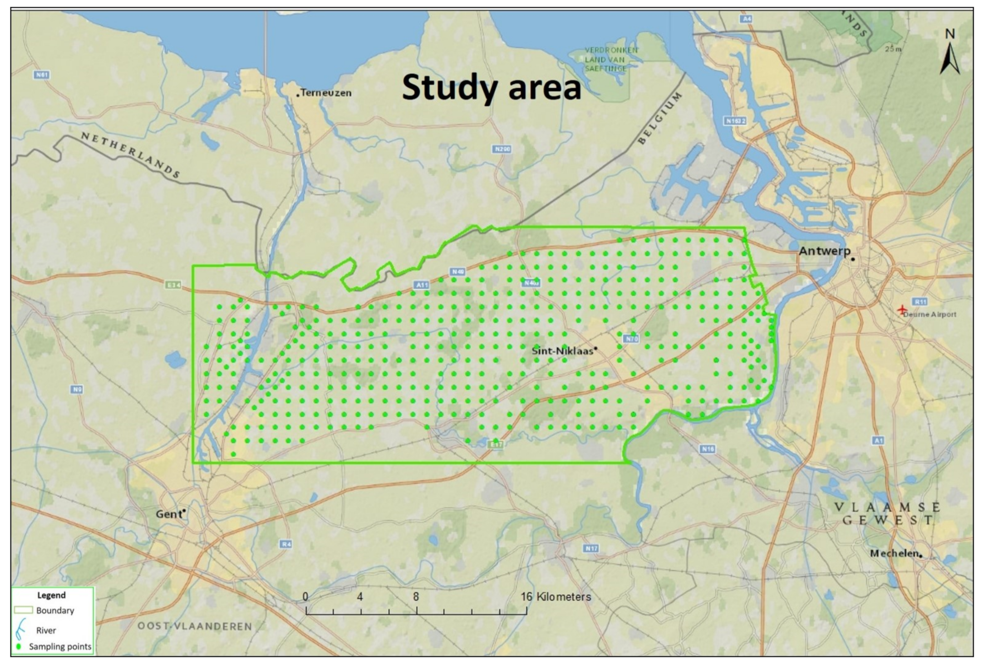
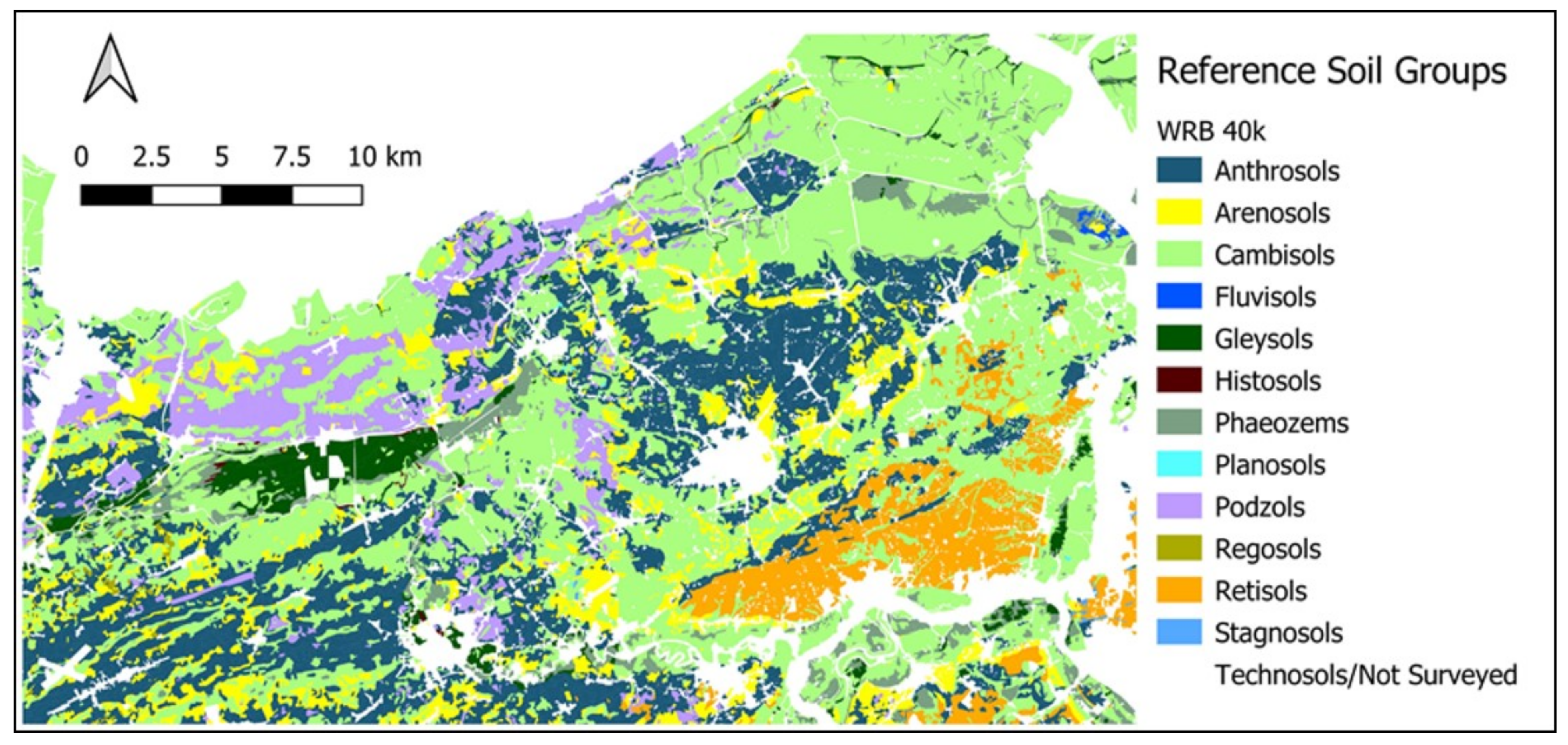
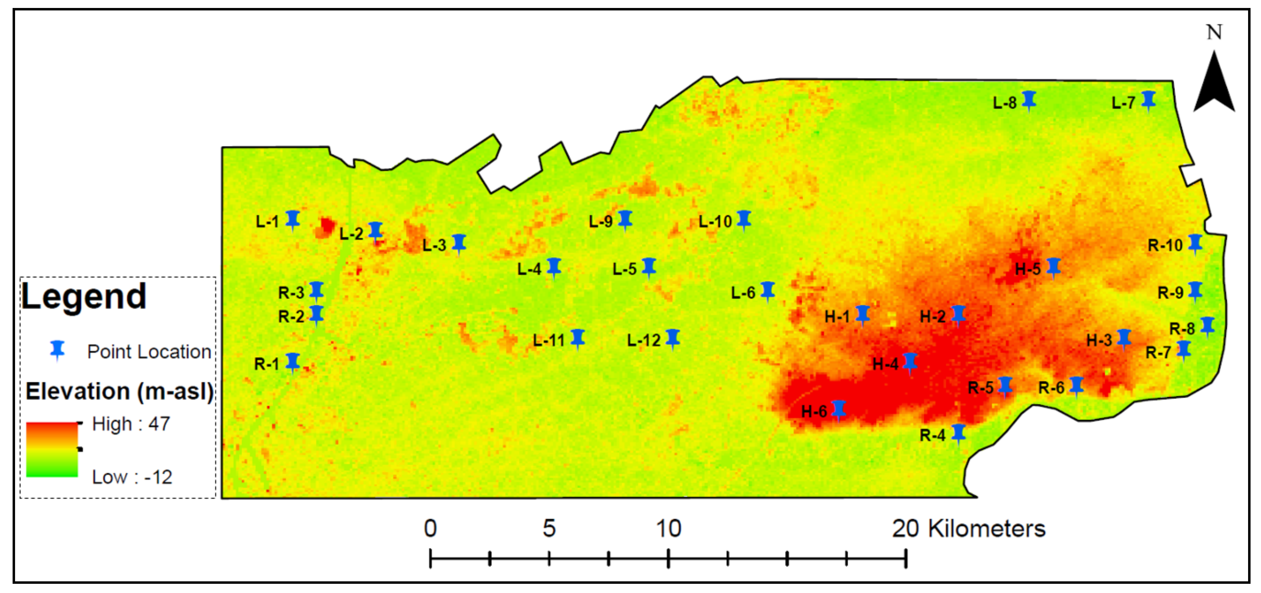
2.1. Study Area and Topsoil Database

The study was conducted over an estimated area of 640 km2 in Northeastern Belgium between the cities of Ghent and Antwerp (Figure 1). A total of 435 soil sampling locations selected from LUCAS database were considered, with a 1 km sampling interval.
Ten HM concentrations (i.e., Sb, Pb, Ni, Mn, Hg, Cu, Cr, Co, Cd and As) were extracted from the Land Use/Cover Area Frame Survey (LUCAS) database, which is an EU-wide project that monitors changes in the management and character of the land surface [21]. The LUCAS topsoil survey provides possibilities to obtain detailed information on soil cover in Europe, including HMs. With its sampling density (1site/200 km2), it is possible to create continuous maps for reliable spatial representation at 1 km resolution of HMs in topsoil of Europe [21]. Details of the soil sampling protocols and soil tests for the HM contents are available in the study of Tóth et al. [1]. The dominant reference soil groups across the study area are Cambisols, Arenosols and Anthrosols (Figure 2). Podzols and Gleysols occur mostly in the northwest and Retisols in the southeast.

2.2. Satellite Data Acquisition and Processing

In this study, satellite data (Landsat 7 imagery with 8 spectral bands) were used as independent variables for building prediction models. From USGS EarthExplorer, four single dates of the Landsat 7 imagery with zero cloud cover were downloaded in the order of 29-05-2009, 05-03-2013, 19-07-2016 and 31-07-2020. The digital number (DN) value of pixels corresponding to the soil sampling locations in each band was converted to spectral reflectance, using ArcMap 10.8.1.

2.3. Data Preparation and Modelling

Exploratory data analyses on the HM concentrations were performed on the 435 extracted points from the LUCAS dataset to identify outliers. Using the quartile–quartile approach, 4.8% of the dataset was detected as an outlier and removed. The new dataset was partitioned (training = 70% and test set = 30%) using the Kennard–Stone algorithm before modeling. The PLSR, RF and SVM models were developed for the soil HM concentrations and the spectral features of the Landsat 7 images. We iterated random 5-fold cross-validation 10 times to counteract both bias and overfitting. In training the models, the coefficient of determination (R2C), the root-mean-square error of calibration (RMSEC), residual prediction deviation (RPDC), and the ratio of performance to the inter-quartile range (RPIQC) were derived to assess how well the regressions fit the training set. The established models were validated using the test set in terms of R2P, RMSEP, RPDP, and RPIQP. To compare the prediction performance of PLSR, RF and SVM models, the model classification scheme based on RPD and proposed by Viscarra Rossel et al. [22] was used. The best performing modeling method for 2009 was subsequently applied to the spectral features for 2013, 2016 and 2020 to assess its transferability and robustness, and allow evaluation of spatiotemporal variation in the studied HMs.
As a linear multivariate regression analysis, PLSR was used. It is a popular multivariate regression method that has a good capacity for estimating attributes resulting from the spectral characteristics of the soil [23]. It is a bilinear modeling method, where information in the original x data is projected onto a small number of underlying (“latent”) variables called PLS components [24]. The y data are actively used in estimating the “latent” variables to ensure that the first components are those that are most relevant for predicting the y variables. Interpretation of the relationship between x data and y data is then simplified, as this relationship is concentrated on the smallest possible number of components. More detailed information about the PLS can be found in the work of Martens and Naes [25]. To determine the optimal number of latent variables, leave-one-out cross-validation (LOOCV) was used [26] to prevent over- or under-fitting the data, which may produce models with poor performance. Generally, a model with the highest cross-validated R2C value and lowest RMSEC value was selected.
As a linear method, SVM is a kernel-based learning method originated from statistical learning theory [27]. These learning methods use an implicit mapping of the input data into a high dimensional feature space defined by a kernel function [28]. The model reduces the complexity of the training data to a significant subset of so-called support vectors. In the current study, two kernels were adopted (second order polynomial and linear kernel) using the R package e1071, and a grid search was conducted by 10-fold cross-validation [29]. The optimal parameters of SVM were adopted so as to produce the best performing model that produced the smallest RMSEC.
RF is a nonparametric and nonlinear classification and regression algorithm first proposed by Ho [30] and further developed by Breiman [31]. It is based on a kind of learning strategy (ensemble learning) that generates many classifiers and aggregates their results. According to its algorithm, RF does not need any data pretreatment, which is one of its main advantages. Tree diversity guarantees RF model stability, which is achieved by two means: (1) a random subset of predictor variables is chosen to grow each tree, or (2) each tree is based on a different random data subset, created by bootstrapping, i.e., sampling with replacement [32]. The RF models were developed using the randomForest package in R with the optimal number of trees to be grown (ntree) and the number of predictor variables used to split the nodes at each partitioning (mtry) set to 500 and 3-times the default mtry value, respectively. The three modeling approaches (PLSR, RF and SVM) were developed with R [33], using the packages ‘prospectr’ [34], ‘e1071′ (Meyer et al., 2015), ‘pls’ [35], ‘randomForest’ [36], and ‘chemometrics’ [37].

2.4. Geostatistical Prediction Method

Ordinary kriging (OK) in ArcGIS software (ArcGIS version 10.7.1, ESRI, Redlands, CA, USA) was employed as the spatial prediction method for mapping the HM distribution in the study area. The input data for the OK were the predicted values of HMs in 2009, 2013, 2016 and 2020, using the best performing models of 2009. Additionally, OK was employed to develop maps of measured HMs. As a geostatistical tool, OK uses the distance between two points to predict the semivariance of the dependent variable. The inter-point semivariances of the spatial data from a measured grid can be used to create a system of linear equations to interpolate the prediction at unmeasured points as a linear function of the measured points. Therefore, for an unmeasured point, linear weights are derived between the unmeasured point and all measured points in the network [38].
In order to explain the variations in HMs over time and space, the study area was classified into three categories: lowlands denoted by ‘L’ (i.e., inland areas), highlands denoted by ‘H’ [i.e., points with elevation >15 m above the sea level (asl)] and river floodplains denoted by ‘R’ (i.e., all points located along the river channels in the study area on the southeast-northeast (SE-NE) boundary and close to the west boundary) (Figure 3 and Table A1).

3. Results

3.1. Soil Heavy Metal Contents

Summary of descriptive statistics of HM concentrations from LUCAS database shows that the coefficient of variation varies between 0.24 and 0.33. Except for Sb, the distribution of HMs concentration showed heavy tails (kurtosis > 3), as compared to the univariate normal distribution (kurtosis = 3). Table 1 summarizes the statistics for all ten HMs.
The Pearson correlations between the ten HMs at a significant level of 0.05 are shown in Figure 4. There are significant positive correlations between all HMs. However, apart from Cr (r = 0.65) and Co (r = 0.66), As reveals a weak positive correlation with the other HMs (r ≤ 0.47). Thus, except for As, there exist strong to very strong correlations (0.60 ≤ r ≤ 1.0) between all HMs.

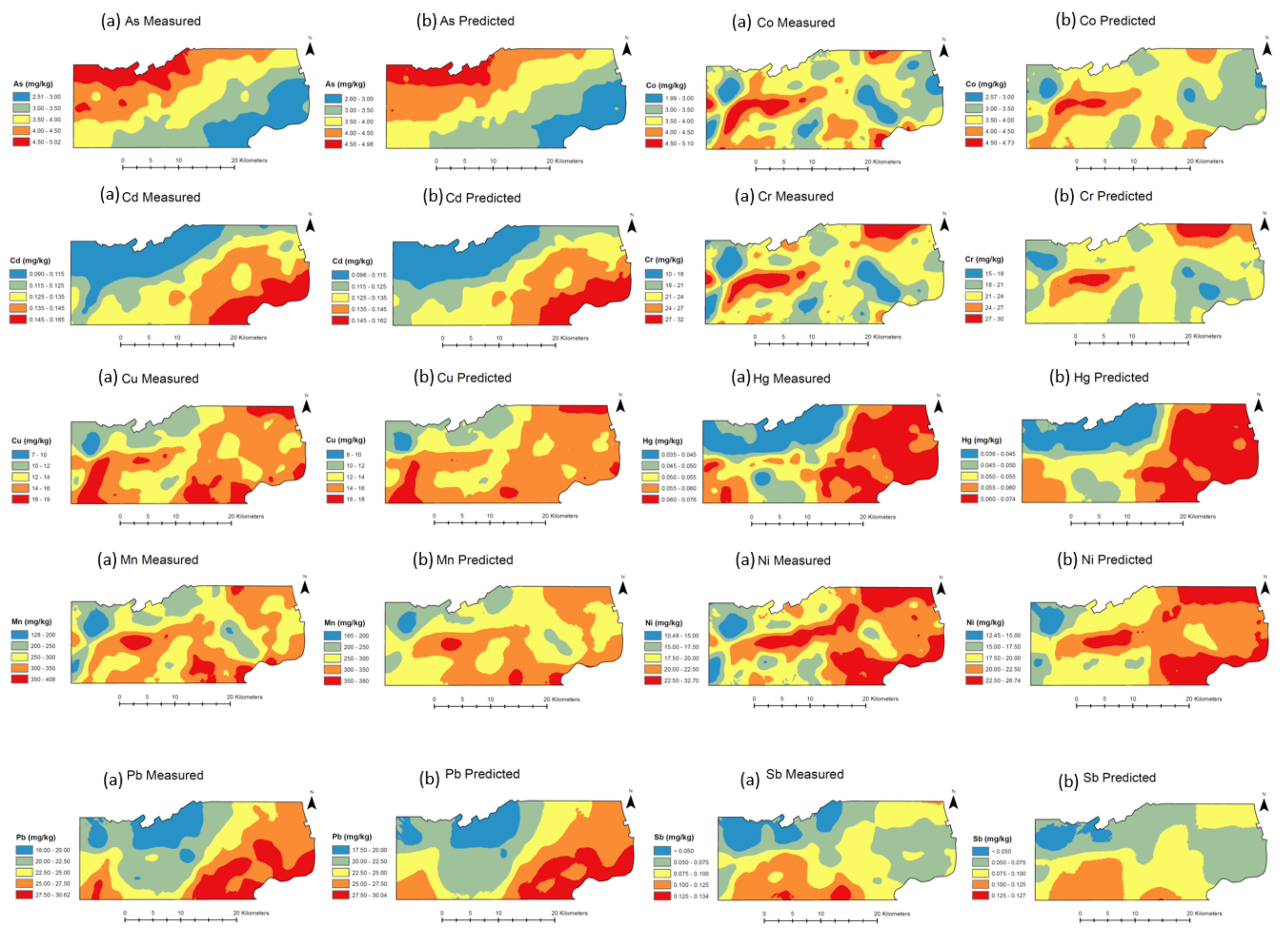
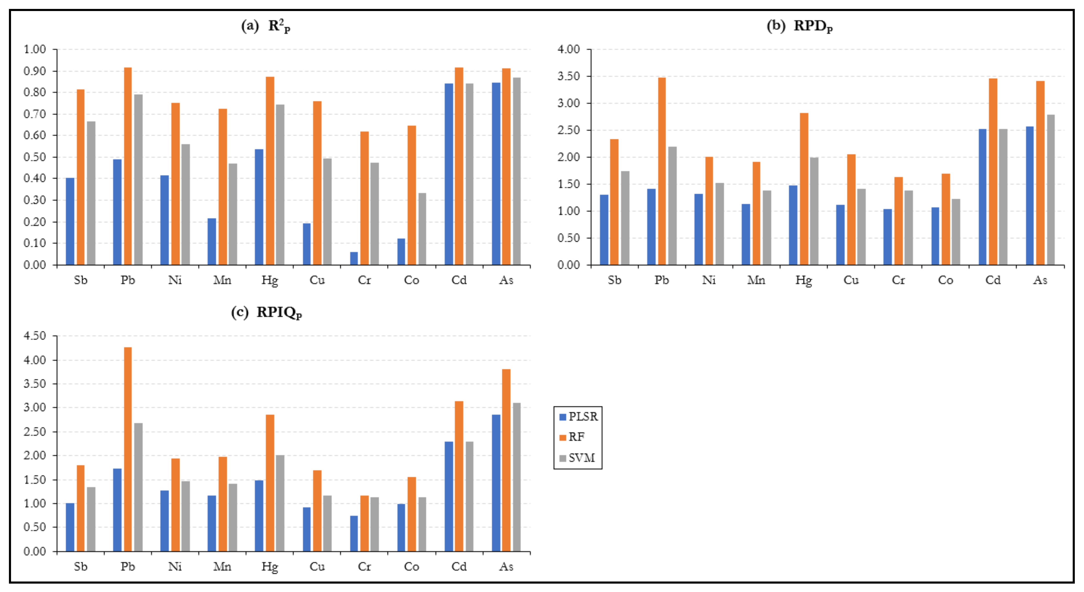
3.2. Comparison in Model Prediction Performance for 2009

The comparison of model prediction performance for PLSR, RF and SVM (with the Gaussian kernel) for 2009 are presented in Figure 5. The two-machine learning algorithms (i.e., RF and SVM) considerably outperformed PLSR in the prediction of all ten HMs that were investigated. In comparison with SVM and PLSR, RF was the best performing model for all ten HMs (0.62 ≤ R2P ≤ 0.92; 1.63 ≤ RPDP ≤ 3.47) followed by SVM with radial kernel (0.33 ≤ R2P ≤ 0.87; 1.23 ≤ RPDP ≤ 2.79) and PLSR (0.06 ≤ R2P ≤ 0.85; 1.12 ≤ RPDP ≤ 2.57). Therefore, RF was selected and used for spatiotemporal prediction and mapping of the HMs for three subsequent years (i.e., 2013, 2016 and 2020). The independent model validation results for PLSR, RF and SVM are detailed in the Appendix A (Table A2).

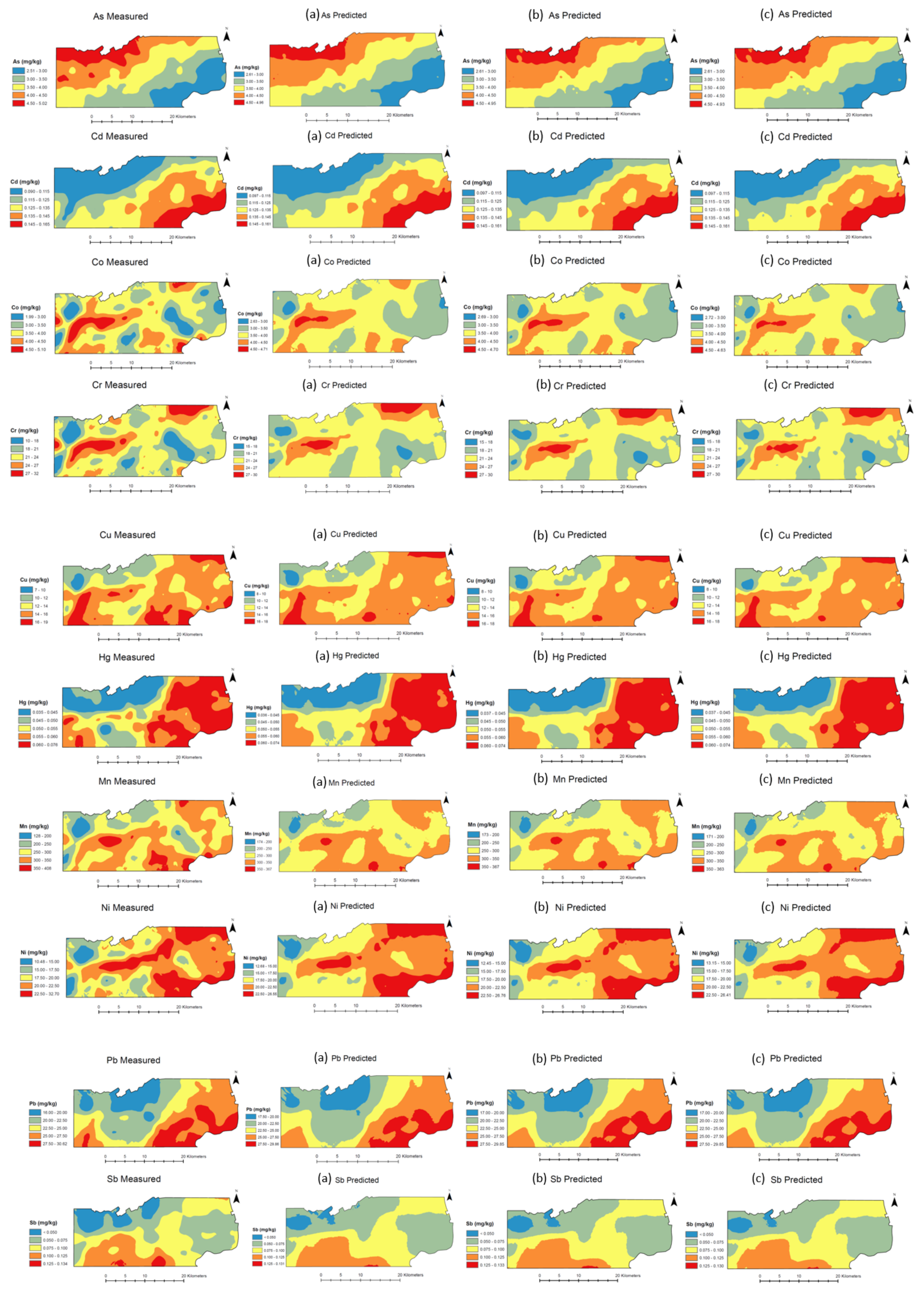
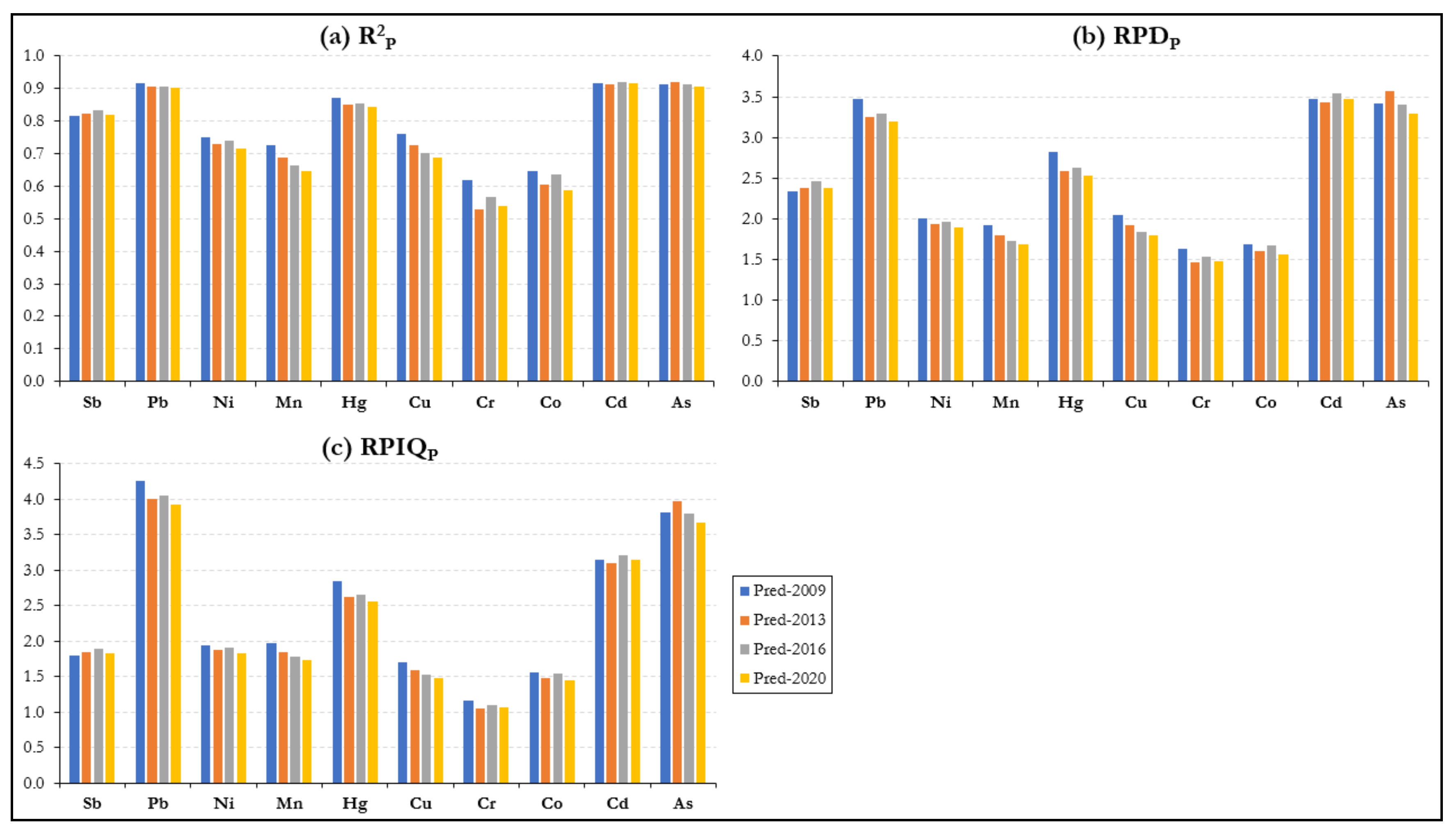
3.3. Spatiotemporal Prediction Performance of RF

The performance of the optimal model (i.e., RF) for 2009 in predicting the HM concentrations for 2013, 2016 and 2020 using only the satellite band reflectance for these three years were analyzed. Figure 6 compares graphically the spatiotemporal prediction performance for the three years as well as 2009. The prediction model statistics (values) are detailed in the Appendix A (Table A3). Apart from Sb, Cd and As, the optimal model results of 2009 for Pb, Ni, Mn, Hg, Cu, Cr and Co outperformed those of 2013, 2016 and 2020. For the seven HMs (Pb, Ni, Mn, Hg, Cu, Cr and Co), the RF prediction performance was decreased over time (Figure 6).

3.4. Spatiotemporal Distribution of Heavy Metals (HMs)

Along the river channel on the SE-NE boundary (Figure 1 and Figure 3), the measured concentrations of Sb, Pb, Ni, Mn, Hg, Cu, Cr, Cd and As increases steadily until after point R-8, where the concentrations sharply decrease. However, the concentration of Co dips sharply at points R-5 and R-10, both of which are located outside the meander of the river. The measured HM concentrations in 2009 at the respective points along the river flood plains exceeded the RF spatiotemporal predicted values, and the latter gradually decreased over time.
In the highlands (Figure 3), the measured concentrations of Pb, Cu and Cd were higher than those recorded in the lowlands (Figure 7). The measured concentrations of Mn and Cd at all the selected points in the highlands randomly alternated in concentrations between high and low. In contrast, high concentrations of Sb, Ni, Mn, Cr, Co and As were recorded in the lowlands, compared to the highlands. However, in the highlands, the RF predicted concentrations of Sb, Ni, Mn Hg, Cr and Co exceeded the measured concentrations in 2009 and increased over time from 2013 to 2020.
The RF predicted concentrations of Cu and As were lower than those measured in the highlands and also decreased over time. Furthermore, the predicted concentrations of Pb and Mn in the lowlands also exceeded the measured values, although the former increased over time from 2013 to 2020, while the latter was generally constant. However, the measured concentrations of Hg, Cu and As exceeded the RF predicted values in the lowlands, although there was no significant variation in the predicted values over time, particularly at L6, L7 and L8, which were located at low elevations (<4.5 m asl) and near the base of the highlands.

3.5. Comparison of Spatiotemporal Distribution Maps

Maps of measured HMs (raw HM extracted data from the LUCAS raster file) and predicted HMs concentration were produced, using OK for interpolation for 2009, 2013, 2016 and 2020 (Figure A1 and Figure A2). Comparison between the measured and predicted maps shows a general decline in the similarity of the HM distribution over time indicated by the kappa values (Figure 8). However, anomalous observations were detected for Sb (kappa = 0.968) and Cd (kappa = 0.984) in 2016, during which a higher similarity (kappa) in the maps was realized.

4. Discussion

4.1. Soil Heavy Metal Contents

In this study, we predicted and mapped the distribution of HM concentrations, using readily accessible Landsat 7 data over a 640 km2 area for years 2009, 2013, 2016 and 2020. The Land Use/Cover Area Frame Survey (LUCAS) database of the study area in the Flemish region of Belgium was used to retrieve the variation in HMs distribution over time and space. The summary of descriptive statistics shows that the coefficient of variation (CV = sd/mean) varies between 0.24 and 0.33 (Table 1), indicating a moderate variation in the HM concentrations, according to Hu et al. [39]. Apart from Sb, the HMs distribution was leptokurtic (kurtosis > 3), as compared to a univariate normal distribution (kurtosis = 3). It indicates the impact of anthropogenic activities on the distribution of HMs in the study area. Factors that affect the HMs distribution in the study area could be pedological factors, agricultural activities, industrial pollution and other anthropogenic activities. Lv et al. [40] reported that anthropogenic activities influence HMs concentration in the soil. Ballabio et al. [41] reported an average concentration of Cu in European topsoil of 16.85 mg/kg, where the main source of Cu in an agricultural soil was the intensive use of pesticides. These results were in line with those of present study, where the average Cu concentration was 13.57 mg/kg. Similarly, Ballabio et al. [42] reported a median Hg concentration of 0.038 mg/kg, which was lower than the 0.055 mg/kg median concentration of Hg in the present study at the non-polluted sites. These differences could be due to spatial variation in HMs distribution and variation in rate of anthropogenic activities at different sites. In another study, Temmerman et al. [43] reported a mean Pb concentration of 21.0 mg/kg and a mean Cu concentration of 10.3 mg/kg in the Flanders region of Belgium, which did not show a significant difference with the measured concentrations of Pb (22.4 mg/kg) and Cu (12.95 mg/kg) in the present study.
Significantly positive correlations were observed between HMs (except for As), which indicate the similar source and origin of HMs in the study area (Figure 3). These results are in line with the findings of previous studies [44,45]. Cr, Co, Ni and Fe have siderophile affinity [46], among which Martín et al. [47] found high correlations. In another study, based on significant positive correlations among Cd, Pb, Co, Mn, Cr and Hg, Lv et al. [40] suggested the similar source of HM pollution in the soil. Positive correlation also explains the comparable modeling results obtained in this work.

4.2. Comparison of Heavy Metals Prediction Performance of Models

Comparison of prediction performance of PLSR, RF and SVM (with the Gaussian kernel) for the dataset of 2009 showed that the RF and SVM considerably outperformed the PLSR in HMs prediction (Figure 5). This result indicates the non-linear relationships between spectra and HMs. However, SVM is a linear regression algorithm, but kernels make it work for nonlinear scenarios. Functions of kernel in the SVM model return the inner product between two points in a suitable feature space; therefore, it defines the notion of similarity, even in the high-dimensional spaces [48]. On the other hand, RF is a non-linear regression method; therefore, it can adequately address the non-linear relationships, compared to PLSR [22]. It makes several different trees by the repeated selection of the subset, and each tree’s deviation is small with large variance. The effect of variance in the overall model is reduced by summing the trees [49]. However, PLSR is a linear regression model, which establishes a linear regression between independent and dependent variables by incorporating principal component matrices. It can partially remove the correlations among variables [50]. In this study, among all three models, RF showed the best performance for all HMs (0.62 ≤ R2P ≤ 0.92; 1.63 ≤ RPDP ≤ 3.47). The suitability of a model for HM detection mainly depends on the inner relationships between spectra and soil HMs [51]. In a previous study, SVM and RF were reported as being the best prediction models for different soil characteristics, as compared to PLSR [52]. In contrast, a study on HM prediction by using Landsat 8 imagery showed that PLSR models performed better than the non-linear regression model (SVM and ANN) [13], which could be due to different soil properties and land use types.
We used RF for the spatiotemporal prediction of HMs for three subsequent years (i.e., 2013, 2016 and 2020), due to its best prediction performance recorded, as compared to SVM and PLSR (Figure 5). Apart from Sb, Cd and As, the prediction efficiency of the RF model for the dataset of 2009 was higher than the datasets for 2013, 2016 and 2020. This outcome was reasonable because the RF model was developed using the dataset of 2009; hence, the RF model achieved the best results for that year. It also could be due to the changes in land use, soil moisture content over time and acquisition date (in 2013, 2016 and 2020) that directly affect the Landsat reflectance spectra [53]. Therefore, it can be assumed that reflectance values of 2009 were different than those obtained for 2013, 2016 and 2020, which can affect the model performance. This means that for the farthest year from the sampling date, the lowest HM models’ prediction performance was recorded. However, the RF spatiotemporal prediction of Sb and Cd for 2016, and As for 2013 were the best, in contrast to 2009 and 2020, which in turn could be attributed to enhanced soil reflectance signatures from the Landsat 7 data during these periods (Figure 5).

4.3. Spatiotemporal Distribution of Heavy Metals and Comparison of Maps

The spatiotemporal distribution of HMS in the study area was classified into three categories: lowlands denoted (L), highlands (H) and river floodplains (R) (Figure 3). Measured concentrations of Sb, Pb, Ni, Mn, Hg, Cu, Cr, Cd and As increased steadily along the river floodplain before point R-8, where the HMs concentration sharply decreased. Compared to L and H, the concentration of Cd at R was relatively higher, which could be due to organic and mineral particles sedimented during frequent flooding periods with low flowrates [54]. Other sources of Cd distribution in the study area could be the application of phosphate fertilizers and atmospheric deposition [55]. Cd input through fertilizer depends on the rate of fertilizer application and the Cd:P2O5 ratio. In 2009, the average atmospheric Cd deposition in Belgium soil was reported to be 0.2 g ha−1 year−1 [56]. Moreover, since the 19th century, several smelting industries, such as Zn smelting, were located in the Flanders region, which produced emissions, causing diffused pollution of HMs in soil [57]. While the concentration of Co sharply decreased at R-5 and R-10, both these points are located outside of the river meander. At these points, sedimentation is low, and the transportation of sediments is high, due to the high flow velocity of the river, which possibly accounts for the low Co concentration. Thus, the increase in SB, Pb, Ni, Mn, Hg, Cu, Cr, Cd and As inside the meander could be due to the low velocity of water and high sedimentation. In previous studies, the significant impact of water flow velocity and sedimentation on HMs transportation was reported [58,59]. Sediment parts (containing HMs) transported to lowlands are transferred with sediment fluxes to the North Sea, which can pollute the marine environment, endanger marine organisms and consequently negatively affect the marine food chain [60].
The measured HM concentrations in 2009 at the respective points along the river channel exceeded the RF spatiotemporal predicted values, and the latter gradually decreased over time. Seasonal variation in the river volume directly affects the soil moisture content in the floodplains. Particularly, since the prediction was based primarily on Landsat 7 reflectance spectra as the independent variable, an increase in the river volume will also increase the soil moisture content in the adjacent floodplains, thus reducing the reflectance spectra. Therefore, the most probable reason accounting for the gradual decrease in the RF predicted HM concentrations along the river channel over time could be an increase in the river volume during the period when the Landsat 7 images for 2013, 2016 and 2020 were taken.
In the highlands, the measured concentrations of Pb, Cu and Cd were higher than those recorded in the lowlands (Figure 7). The measured concentrations of Mn and Cd at all the selected points in the highlands alternated in concentration between high and low. In the study area, there were four gas stations located in the highlands and close to the points X-8, X-20 and X-21. Moreover, since Pb, Cu, Cd and Mn are trace metals in petroleum, a high concentration of these metals in the highlands originated most likely from soil contamination by the petroleum from the gas stations. In contrast, high concentrations of Sb, Ni, Mn, Cr, Co and As were recorded in the lowlands, compared to the highland, which could be due to erosion, transportation and the deposition of petroleum-contaminated soils from the highland areas into the lowlands aided by rainfall, snowmelt and wind. In the highlands, the RF-predicted concentrations of Sb, Ni, Mn Hg, Cr and Co exceeded the measured concentrations in 2009 and increased over time from 2013 to 2020 due to the enhanced reflectance spectra, which could be attributed to a reduction in the soil moisture content in the highlands over time. The sun’s azimuth in the study area decreased from 156.6° (in 2013), 149.9° (in 2016) to 148.6° (in 2020), but in 2009 it was 146.6°. Weather patterns during data acquisition could be another reason. A decrease in the sun’s azimuth is reciprocal to an increase in solar insolation and, hence, an increase in evapotranspiration, which will eventually result in a reduction in moisture content. Therefore, a reduction in the soil moisture content in the highlands over time enhanced the soil reflectance spectra, which could account for the increase in RF-predicted concentrations of HMs [61]. The measured concentrations of Cu and As in the highlands exceeded the RF-predicted concentrations. In the lowlands, the measured concentrations of Pb and Mn were lower than the RF-predicted values. It could be due to an increase in the reflectance spectra within the lowlands as a result of the decrease in the sun’s azimuth and the decrease in moisture content, and perhaps partially due to a decline of natural drainage. In the lowlands, RF-predicted values of Hg, Cu and As were lower, compared to the measured concentrations, and did not show significant differences among the years. Particularly, L6, L7 and L8 were located at low elevations (<4.5 m asl) and near the base of the highlands. Such locations are prone to sedimentation from the highlands during rainfall and snowmelt when the topsoil is eroded, transported and deposited into the lowlands. Thus, the major driving factors of HMs accumulation in the region could be changes in moisture content due to evapotranspiration, variation in waterflow velocity, affecting HMs transportation from highlands to lowlands, sedimentation and changes in weather conditions over time, i.e., rainfall. However, apart from climate and topographic factors, anthropogenic activities, such as agricultural and mining activities and land use management, could be among major factors of HM accumulation in the study area. For example, the application of Cu-containing fungicide in agricultural soil is considered one of the major sources of Cu accumulation in European soils [62]. In another study, Qaswar et al. [63] found that the long-term application of fertilizers increased Cd, Hg and Cr concentrations in agricultural soils. Land use change alters the hydrological process and influences the transportation of HMs in soil [64]. Moreover, soil pH and organic matter distribution significantly affect the accumulation of HMs in soils [42].
Maps were produced for measured and predicted concentrations of HMs, using OK interpolation method (Figure A1 and Figure A2). The predicted maps show that similarity of HMs distribution was decreased over the time in the study area. These variations in the spatial distribution are attributed to changes in the weather conditions over time that change the Landsat 7 spectral reflectance [65]. Moreover, spatial similarity, evaluated according to Kappa values of 2009 were higher than those obtained for 2013, 2016 and 2020 (Figure 8). That might be due to the high accuracy of the RF prediction of the 2009 dataset, compared to the corresponding predictions in 2013, 2016 and 2020, using the 2009 models. Thus, the RF models for spatiotemporal prediction of HMs using Landsat 7 spectral reflectance could be regarded as the best method that can be used for monitoring and management of HMs contaminated sites. This will allow observing spatiotemporal differences and understand the reasons of these differences.

5. Conclusions

The testing of different models (including linear and non-linear) and model selection as well as unbiased evaluation of the models are imperative to achieve and improve the prediction accuracy of HMs in soils when using satellite data. In this study, we found that Landsat 7 satellite data coupled with RF show great potential for predicting and mapping the spatiotemporal distribution of Sb, Pb, Ni, Mn, Hg, Cu, Cr, Co, Cd and As in soils at regional scale. The R2P and RPDP achieved by RF for all the HMs ranged from 0.62 to 0.92, and 1.23 to 2.79, respectively. This could be classified as a high performing model for spatiotemporal prediction in contrast to PLSR and SVM.
High concentrations of the measured HMs were detected inside the meanders of the floodplains. These locations are characterized by low river flow velocity, which creates a conducive environment for high river sedimentation. Therefore, sediments with HMs adsorbed onto their surface were readily deposited inside the meander, resulting in high HM concentrations. The RF predicted concentrations along the river channel decreased over time (from 2009, 2013, 2016 to 2020), largely due to the seasonal increase in the river volume, which also increased the moisture content in the floodplains and hence, reduced the reflectance spectra from the floodplains. In the highlands, the measured concentration of HMs exceeded the RF-predicted concentration over time, which is attributed to reduced Landsat 7 spectral reflectance, due to increases in the moisture content in the highlands. Moreover, high concentration of measured HMs in the highlands also could be due to the presence of gas stations in the highlands. Similarly, high concentrations of measured HMs were detected in the lowlands, but these decreased over time when predicted with the RF model. Comparison between the measured and predicted maps showed a general decline in the similarity of the HM spatial distribution over time in the study area. Thus, we concluded that RF model for spatiotemporal prediction of HMs using Landsat 7 spectral reflectance could be regarded as an efficient method, which can be helpful to monitor the large HM contaminated areas for mitigation strategies. Future research will need to consider multiple years before 2009 to ascertain the robustness of the RF model as well as assess the variations and similarities in the spatiotemporal distribution of the HMs in the study area.

Author Contributions

Conceptualization, A.M.M. and F.N.; methodology, F.N.; software, F.N.; validation, F.N. and A.M.M.; data curation, G.T.; writing—original draft preparation, A.M.M.; writing—review and editing, A.G., G.T. and M.Q.; visualization, F.N.; supervision, A.M.M.; project administration, D.M.; funding acquisition, D.M. and A.M.M. All authors have read and agreed to the published version of the manuscript.

Funding

This research was funded by the European Commission, grant number 818346 called Sino-EU Soil Observatory for intelligent Land Use Management (SIEUSOIL).

Institutional Review Board Statement

Not applicable.

Informed Consent Statement

Not applicable.

Data Availability Statement

The datasets generated during and/or analyzed during the current study are available from the corresponding author on reasonable request. The satellite data are available at the European Soil Data Centre (ESDAC), European Commission, Joint Research Centre.

Conflicts of Interest

The authors declare no conflict of interest.

Appendix A

Table A1. Selected points for spatiotemporal mapping and their corresponding elevations (m) above sea level (asl).
Sampling PointsElevation (m asl *)
L-12.2
L-212.7
L-32.8
L-44.2
L-51.0
L-64.3
L-7−2.3
L-8−1.0
L-93.4
L-101.8
L-112.0
L-121.8
H-115.0
H-223.9
H-318.4
H-429.3
H-517.0
H-630.4
R-13.0
R-20.0
R-30.0
R-43.9
R-523.2
R-613.8
R-73.9
R-8−0.6
R-92.3
R-107.2
* masl: meters above sea-level.
Table A2. Comparison in prediction performance of partial least squares regression (PLSR), random forest (RF) and support vector machine (SVM), using the independent set of the 2009 data.
PLSRRFSVM
HMsLVR2pRMSEP (mg/kg) RPDRPIQR2pRMSEP
(mg/kg)
RPDRPIQNo. SVR2pRMSEP
(mg/kg)
RPDRPIQ
Sb70.410.021.301.000.810.0092.331.802420.670.0121.741.34
Pb40.492.221.401.720.920.8973.474.272220.791.4252.192.69
Ni40.412.371.311.270.751.5492.011.952680.562.0551.511.47
Mn60.2238.151.131.170.7322.5721.921.972600.4731.3451.381.42
Hg50.540.011.471.490.870.0032.822.852480.740.0051.992.01
Cu40.191.821.120.930.760.9912.051.702440.491.4401.411.17
Cr20.063.201.040.740.622.0381.631.172560.482.1011.391.13
Co20.120.501.070.990.650.3211.691.562590.330.4401.231.14
Cd50.840.012.522.290.920.0043.473.142240.840.0062.522.29
As50.850.222.572.860.910.163.423.812310.870.2032.783.10
Table A3. Comparison in random forest (RF) models’ spatiotemporal prediction performance for the years 2009, 2013, 2016 and 2020.
HMs2009201320162020
HMsR2PRMSEP
(mg/kg)
RPDPRPIQPR2PRMSEP
(mg/kg)
RPDPRPIQPR2PRMSEP
(mg/kg)
RPDPRPIQPR2PRMSEP
(mg/kg)
RPDPRPIQP
Sb0.810.0092.331.800.820.012.381.840.830.012.461.890.820.012.371.83
Pb0.920.8973.474.270.910.963.264.000.910.953.294.050.900.973.201.93
Ni0.751.5492.011.950.731.611.931.870.741.581.971.900.721.651.891.83
Mn0.7322.5721.921.970.6924.041.801.850.6624.941.731.780.6525.621.691.74
Hg0.870.0032.822.850.850.002.592.620.850.002.622.660.840.002.532.56
Cu0.760.9912.051.700.731.061.921.590.701.101.841.530.691.131.791.49
Cr0.622.0381.631.170.532.261.471.050.572.171.531.090.542.241.481.06
Co0.650.3211.691.560.610.341.601.480.640.321.671.540.590.351.561.45
Cd0.920.0043.473.140.910.003.433.110.920.003.543.210.920.003.483.15
As0.910.163.423.810.920.163.573.980.910.173.413.410.910.173.303.67
Figure A1. Spatial distribution and comparison between measured (a) and random forest (RF)–predicted (b) maps developed with ordinary kriging (OK) for different heavy metals (HMs) over the study area for the year 2009.
Remotesensing 13 04615 g0a1
Figure A2. Spatial distribution and comparison between measured and random forest (RF)–predicted maps using ordinary kriging (OK) for different heavy metals (HMs) over the study area for the years 2013 (a), 2016 (b) and 2020 (c).
Remotesensing 13 04615 g0a2

References

  1. Tóth, G.; Hermann, T.; Szatmári, G.; Pásztor, L. Maps of heavy metals in the soils of the European Union and proposed priority areas for detailed assessment. Sci. Total Environ. 2016, 565, 1054–1062. [Google Scholar] [CrossRef] [PubMed]
  2. Micó, C.; Peris, M.; Recatalá, L.; Sánchez, J. Baseline values for heavy metals in agricultural soils in an European Mediterranean region. Sci. Total Environ. 2007, 378, 13–17. [Google Scholar] [CrossRef]
  3. Hudcová, H.; Vymazal, J.; Rozkošný, M. Present restrictions of sewage sludge application in agriculture within the European Union. Soil Water Res. 2019, 14, 104–120. [Google Scholar] [CrossRef]
  4. Alengebawy, A.; Abdelkhalek, S.T.; Qureshi, S.R.; Wang, M.-Q. Heavy metals and pesticides toxicity in agricultural soil and plants: Ecological risks and human health implications. Toxics 2021, 9, 42. [Google Scholar] [CrossRef]
  5. Van Liedekerke, M.; Prokop, G.; Rabl-Berger, S.; Kibblewhite, M.; Louwagie, G. Progress in Management of Contaminated Sites in Europe; JRC Technical Reports; Publications Office of the European Union: Luxembourg, 2014. [Google Scholar]
  6. Lima, A.T.; Safar, Z.; Loch, J.P.G. Evaporation as the transport mechanism of metals in arid regions. Chemosphere 2014, 111, 638–647. [Google Scholar] [CrossRef]
  7. Liu, Y.; Li, W.; Wu, G.; Xu, X. Feasibility of estimating heavy metal contaminations in floodplain soils using laboratory-based hyperspectral data—A case study along Le’an River, China. Geo-Spatial Inf. Sci. 2011, 14, 10–16. [Google Scholar] [CrossRef] [Green Version]
  8. Slonecker, T.; Fisher, G.B.; Aiello, D.P.; Haack, B. Visible and infrared remote imaging of hazardous waste: A review. Remote Sens. 2010, 2, 2474–2508. [Google Scholar] [CrossRef] [Green Version]
  9. Von Steiger, B.; Webster, R.; Schulin, R.; Lehmann, R. Mapping heavy metals in polluted soil by disjunctive kriging. Environ. Pollut. 1996, 94, 205–215. [Google Scholar] [CrossRef]
  10. Kemper, T.; Sommer, S. Estimate of heavy metal contamination in soils after a mining accident using reflectance spectroscopy. Environ. Sci. Technol. 2002, 36, 2742–2747. [Google Scholar] [CrossRef]
  11. Ji, J.; Song, Y.; Yuan, X.; Yang, Z. Diffuse reflectance spectroscopy study of heavy metals in agricultural soils of the Changjiand River Delta, China. In Proceedings of the 19th World Congress of Soil Science, Soil Solutions for a Changing World, Brisbane, Australia, 1–6 August 2010; pp. 47–50. [Google Scholar]
  12. Fard, R.S.; Matinfar, H.R. Capability of vis-NIR spectroscopy and Landsat 8 spectral data to predict soil heavy metals in polluted agricultural land (Iran). Arab. J. Geosci. 2016, 9, 1–14. [Google Scholar]
  13. Fang, Y.; Xu, L.; Peng, J.; Wang, H.; Wong, A.; Clausi, D.A. Retrieval and mapping of heavy metal concentration in soil using time series landsat 8 imagery. Int. Arch. Photogramm. Remote Sens. Spat. Inf. Sci. ISPRS Arch. 2018, 42, 335–340. [Google Scholar] [CrossRef] [Green Version]
  14. Junliang, H.; Shuyuan, Z.; Yong, Z.; Jianjun, J. Review of retrieving soil heavy metal content by hyperspectral remote sensing. Remote Sens. Technol. Appl. 2015, 30, 407–412. [Google Scholar]
  15. Riedel, F.; Denk, M.; Müller, I.; Barth, N.; Gläßer, C. Prediction of soil parameters using the spectral range between 350 and 15,000 nm: A case study based on the Permanent Soil Monitoring Program in Saxony, Germany. Geoderma 2018, 315, 188–198. [Google Scholar] [CrossRef]
  16. Cheng, H.; Shen, R.; Chen, Y.; Wan, Q.; Shi, T.; Wang, J.; Wan, Y.; Hong, Y.; Li, X. Estimating heavy metal concentrations in suburban soils with reflectance spectroscopy. Geoderma 2019, 336, 59–67. [Google Scholar] [CrossRef]
  17. Al Maliki, A.; Owens, G.; Bruce, D. Capabilities of remote sensing hyperspectral images for the detection of lead contamination: A review. ISPRS Ann. Photogramm. Remote Sens. Spat. Inf. Sci. 2012, 1, 55–60. [Google Scholar] [CrossRef] [Green Version]
  18. Huang, X.; Senthilkumar, S.; Kravchenko, A.; Thelen, K.; Qi, J. Total carbon mapping in glacial till soils using near-infrared spectroscopy, Landsat imagery and topographical information. Geoderma 2007, 141, 34–42. [Google Scholar] [CrossRef]
  19. Zhou, T.; Geng, Y.; Ji, C.; Xu, X.; Wang, H.; Pan, J.; Bumberger, J.; Haase, D.; Lausch, A. Prediction of soil organic carbon and the C:N ratio on a national scale using machine learning and satellite data: A comparison between Sentinel-2, Sentinel-3 and Landsat-8 images. Sci. Total Environ. 2021, 755, 142661. [Google Scholar] [CrossRef] [PubMed]
  20. Ali, I.; Greifeneder, F.; Stamenkovic, J.; Neumann, M.; Notarnicola, C. Review of Machine Learning Approaches for Biomass and Soil Moisture Retrievals from Remote Sensing Data. Remote Sens. 2015, 7, 16398–16421. [Google Scholar] [CrossRef] [Green Version]
  21. Tóth, G.; Jones, A.; Montanarella, L. LUCAS Topsoil Survey: Methodology, Data, and Results; JRC Technical Reports; Publications Office: Luxembourg, 2013; ISBN 9789279325427. [Google Scholar]
  22. Viscarra Rossel, R.A.V.; Walvoort, D.J.J.; McBratney, A.B.; Janik, L.J.; Skjemstad, J.O. Visible, near infrared, mid infrared or combined diffuse reflectance spectroscopy for simultaneous assessment of various soil properties. Geoderma 2006, 131, 59–75. [Google Scholar] [CrossRef]
  23. Song, Y.; Ji, J.; Mao, C.; Ayoko, G.A.; Frost, R.L.; Yang, Z.; Yuan, X. The use of reflectance visible-NIR spectroscopy to predict seasonal change of trace metals in suspended solids of Changjiang River. Catena 2013, 109, 217–224. [Google Scholar] [CrossRef]
  24. Mouazen, A.M.; De Baerdemaeker, J.; Ramon, H. Effect of wavelength range on the measurement accuracy of some selected soil constituents using visual-near infrared spectroscopy. J. Near Infrared Spectrosc. 2006, 14, 189–199. [Google Scholar] [CrossRef]
  25. Martens, H.; Naes, T. Assessment, validation and choice of calibration method. In Multivariate Calibration; John Wiley & Sons: Hoboken, NJ, USA, 1989; pp. 237–266. [Google Scholar]
  26. Efron, B.; Tibshiran, R. (Eds.) An Introduction to the Bootstrap; Chapman &Hall, Inc.: London, UK, 1993. [Google Scholar]
  27. Vapnik, V.; Guyon, I.; Hastie, T. Support vector machines. Mach. Learn. 1995, 20, 273–297. [Google Scholar]
  28. Karatzoglou, A.; Feinerer, I. Kernel-based machine learning for fast text mining in R. Comput. Stat. Data Anal. 2010, 54, 290–297. [Google Scholar] [CrossRef]
  29. Meyer, D.; Wien, F.H.T. Support vector machines. In Interface Libsvm Package E1071; FH Technikum Wien: Vienna, Austria, 2015; pp. 1–28. [Google Scholar]
  30. Ho, T.K. The random subspace method for constructing decision forests. IEEE Trans. Pattern Anal. Mach. Intell. 1998, 20, 832–844. [Google Scholar]
  31. Breiman, L. Random forests. Mach. Learn. 2001, 45, 5–32. [Google Scholar] [CrossRef] [Green Version]
  32. Efron, B. Computers and the theory of statistics: Thinking the unthinkable. SIAM Rev. 1979, 21, 460–480. [Google Scholar] [CrossRef]
  33. R Foundation for Statistical Computing. R Core Team A Language and Environment for Statistical Computing; R Foundation for Statistical Computing: Vienna, Austria, 2020. [Google Scholar]
  34. Stevens, A.; Ramirez-Lopez, L. Package Vignette. In An Introduction to the Prospectr Package; R Package Version 0.2.0; University of Liege: Liege, Belgium, 2020; pp. 1–22. [Google Scholar]
  35. Wehrens, R. pls: Partial Least Squares Regression (PLSR) and Principal Component Regression (PCR). R Package Ver. 2.0-0. 2006. Available online: http//mevik.net/work/software/pls.html (accessed on 30 March 2021).
  36. Zaremba, L.S.; Smoleński, W.H. Optimal portfolio choice under a liability constraint. Ann. Oper. Res. 2000, 97, 131–141. [Google Scholar] [CrossRef]
  37. Garcia, H.; Filzmoser, P. Multivariate Statistical Analysis Using the R Package Chemometrics; Vienna University of Technology: Vienna, Austria, 2011; pp. 1–71. [Google Scholar]
  38. Farmer, W.H. Ordinary kriging as a tool to estimate historical daily streamflow records. Hydrol. Earth Syst. Sci. 2016, 20, 2721–2735. [Google Scholar] [CrossRef] [Green Version]
  39. Hu, B.; Chen, S.; Hu, J.; Xia, F.; Xu, J.; Li, Y.; Shi, Z. Application of portable XRF and VNIR sensors for rapid assessment of soil heavy metal pollution. PLoS ONE 2017, 12, e0172438. [Google Scholar] [CrossRef] [Green Version]
  40. Lv, J.; Liu, Y.; Zhang, Z.; Dai, J.; Dai, B.; Zhu, Y. Identifying the origins and spatial distributions of heavy metals in soils of Ju country (Eastern China) using multivariate and geostatistical approach. J. Soils Sediments 2015, 15, 163–178. [Google Scholar] [CrossRef]
  41. Ballabio, C.; Panagos, P.; Lugato, E.; Huang, J.-H.; Orgiazzi, A.; Jones, A.; Fernández-Ugalde, O.; Borrelli, P.; Montanarella, L. Copper distribution in European topsoils: An assessment based on LUCAS soil survey. Sci. Total Environ. 2018, 636, 282–298. [Google Scholar] [CrossRef] [PubMed]
  42. Ballabio, C.; Jiskra, M.; Osterwalder, S.; Borrelli, P.; Montanarella, L.; Panagos, P. A spatial assessment of mercury content in the European Union topsoil. Sci. Total Environ. 2021, 769, 144755. [Google Scholar] [CrossRef]
  43. De Temmerman, L.; Vanongeval, L.; Boon, W.; Hoenig, M.; Geypens, M. Heavy metal content of arable soils in Northern Belgium. Water Air Soil Pollut. 2003, 148, 61–76. [Google Scholar] [CrossRef]
  44. Cai, L.; Xu, Z.; Ren, M.; Guo, Q.; Hu, X.; Hu, G.; Wan, H.; Peng, P. Source identification of eight hazardous heavy metals in agricultural soils of Huizhou, Guangdong Province, China. Ecotoxicol. Environ. Saf. 2012, 78, 2–8. [Google Scholar] [CrossRef]
  45. Micó, C.; Recatalá, L.; Peris, M.; Sánchez, J. Assessing heavy metal sources in agricultural soils of an European Mediterranean area by multivariate analysis. Chemosphere 2006, 65, 863–872. [Google Scholar] [CrossRef] [PubMed]
  46. Alloway, B.J. Heavy Metals in Soils: Trace Metals and Metalloids in Soils and Their Bioavailability; Springer: Heidelberg, The Netherlands, 2012; Volume 22, ISBN 978-0-7514-0198-1. [Google Scholar]
  47. Martín, J.A.R.; Arias, M.L.; Corbí, J.M.G. Heavy metals contents in agricultural topsoils in the Ebro basin (Spain). Application of the multivariate geoestatistical methods to study spatial variations. Environ. Pollut. 2006, 144, 1001–1012. [Google Scholar] [CrossRef]
  48. Karatzoglou, A.; Meyer, D.; Hornik, K. Support vector algorithm in R. J. Stat. Softw. 2006, 15, 1–28. [Google Scholar] [CrossRef] [Green Version]
  49. Tan, K.; Ma, W.; Wu, F.; Du, Q. Random forest–based estimation of heavy metal concentration in agricultural soils with hyperspectral sensor data. Environ. Monit. Assess. 2019, 191, 446. [Google Scholar] [CrossRef]
  50. Wold, S. Personal memories of the early PLS development. Chemom. Intell. Lab. Syst. 2001, 58, 83–84. [Google Scholar] [CrossRef]
  51. Gholizadeh, A.; Borůvka, L.; Saberioon, M.M.; Kozak, J.; Vašát, R.; Němeček, K. Comparing different data preprocessing methods for monitoring soil heavy metals based on soil spectral features. Soil Water Res. 2015, 10, 218–227. [Google Scholar] [CrossRef] [Green Version]
  52. Wenjun, J.; Zhou, S.; Jingyi, H.; Shuo, L. In situ measurement of some soil properties in paddy soil using visible and near-infrared spectroscopy. PLoS ONE 2014, 9, e105708. [Google Scholar]
  53. Fu, P.; Weng, Q. A time series analysis of urbanization induced land use and land cover change and its impact on land surface temperature with Landsat imagery. Remote Sens. Environ. 2016, 175, 205–214. [Google Scholar] [CrossRef]
  54. Devai, I.; Patrick, W.H., Jr.; Neue, H.; De Laune, R.D.; Kongchum, M.; Rinklebe, J. Methyl mercury and heavy metal content in soils of rivers Saale and Elbe (Germany). Anal. Lett. 2005, 38, 1037–1048. [Google Scholar] [CrossRef]
  55. Six, L.; Smolders, E. Future trends in soil cadmium concentration under current cadmium fluxes to European agricultural soils. Sci. Total Environ. 2014, 485–486, 319–328. [Google Scholar] [CrossRef]
  56. Travnikov, O.; Ilyin, I.; Rozovskaya, O.; Varygina, M.; Aas, W.; Uggerud, H.T.; Mareckova, K.; Wankmueller, R. Long-term changes of heavy metal transboundary pollution of the environment (1990–2010). EMEP Status Rep. 2012, 2, 1–63. [Google Scholar]
  57. Gentile, A.R.; Barceló-Cordón, S.; Van Liedekerke, M. Soil Country Analyses-Belgium; JRC: Ispra, Italy, 2009; ISBN 9789279133510. [Google Scholar]
  58. Kashefipour, S.M.; Roshanfekr, A. Numerical modelling of heavy metals transport processes in riverine basins. Numer. Model. 2012, 6, 66–69. [Google Scholar]
  59. Yan, H.; Zhang, H.; Shi, Y.; Ping, Z.; Huan, L.I.; Wu, D.; Liu, L.I.U. Simulation on release of heavy metals Cd and Pb in sediments. Trans. Nonferrous Met. Soc. China 2021, 31, 277–287. [Google Scholar] [CrossRef]
  60. Förstner, U.; Müller, G. Heavy metal accumulation in river sediments: A response to environmental pollution. Geoforum 1973, 4, 53–61. [Google Scholar] [CrossRef]
  61. Yi, Z.; Liu, M.; Liu, X.; Wang, Y.; Wu, L.; Wang, Z.; Zhu, L. Long-term Landsat monitoring of mining subsidence based on spatiotemporal variations in soil moisture: A case study of Shanxi Province, China. Int. J. Appl. Earth Observ. Geoinf. 2021, 102, 102447. [Google Scholar] [CrossRef]
  62. Qaswar, M.; Yiren, L.; Jing, H.; Kaillou, L.; Mudasir, M.; Zhenzhen, L.; Hongqian, H.; Xianjin, L.; Jianhua, J.; Ahmed, W.; et al. Soil nutrients and heavy metal availability under long-term combined application of swine manure and synthetic fertilizers in acidic paddy soil. J. Soils Sediments 2020, 20, 2093–2106. [Google Scholar] [CrossRef]
  63. Zhang, Y.; Zhang, X.; Bi, Z.; Yu, Y.; Shi, P.; Ren, L.; Shan, Z. The impact of land use changes and erosion process on heavy metal distribution in the hilly area of the Loess Plateau, China. Sci. Total Environ. 2020, 718, 137305. [Google Scholar] [CrossRef] [PubMed]
  64. Xiao, W.; Lin, G.; He, X.; Yang, Z.; Wang, L. Interactions among heavy metal bioaccessibility, soil properties and microbial community in phyto-remediated soils nearby an abandoned realgar mine. Chemosphere 2022, 286, 131638. [Google Scholar] [CrossRef] [PubMed]
  65. Mohamed, E.S.; Baroudy, A.; El-beshbeshy, T.; Emam, M.; Belal, A.A.; Elfadaly, A.; Aldosari, A.A.; Ali, A.; Lasaponara, R. Vis-NIR Spectroscopy and Satellite Landsat-8 OLI Data to Map Soil Nutrients in Arid Conditions: A Case Study of the Northwest Coast of Egypt. Remote Sens. 2020, 12, 3716. [Google Scholar] [CrossRef]
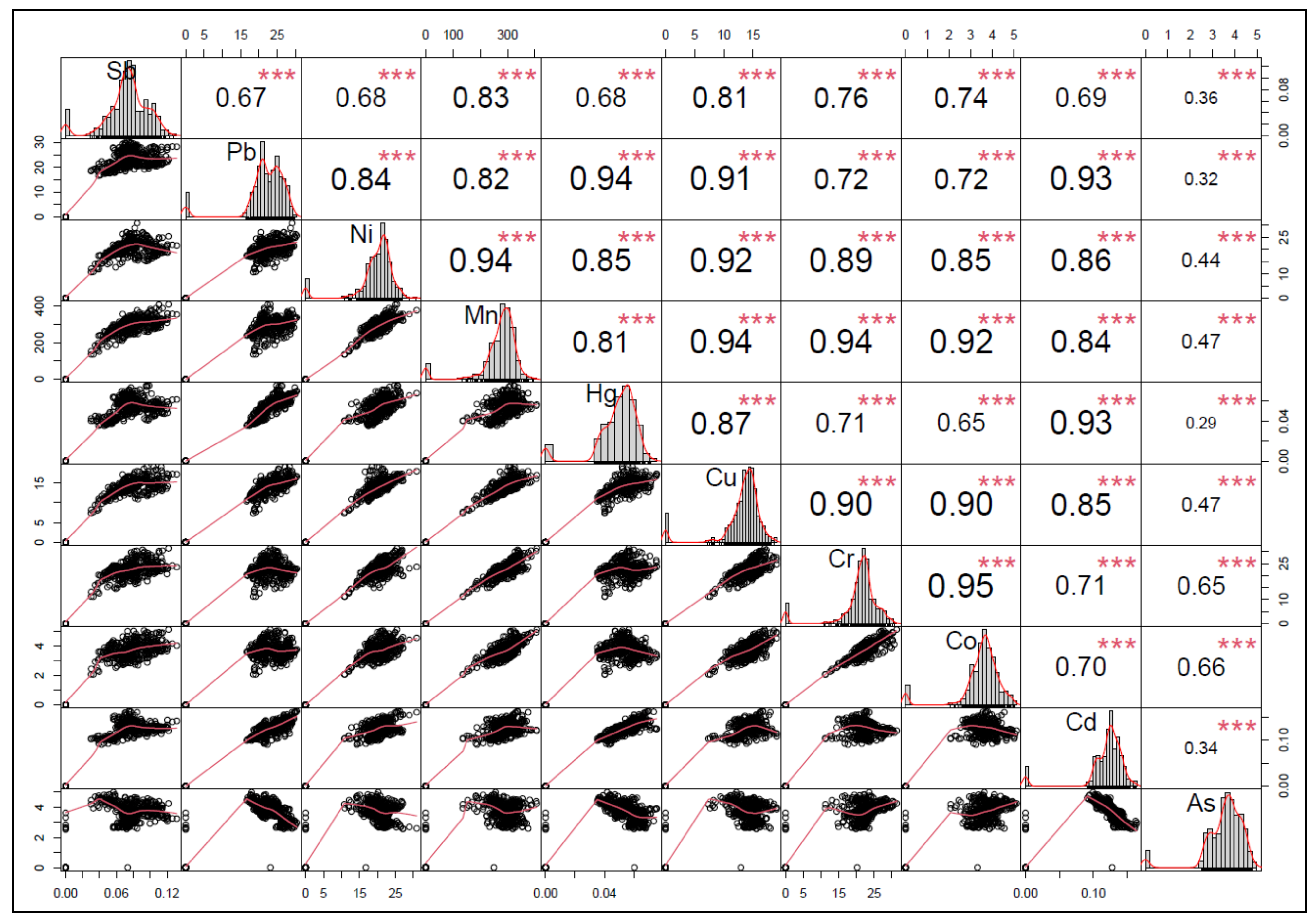
Figure 1. Geographical map of study area.
Remotesensing 13 04615 g001
Figure 2. Reference soil groups of the study area. World reference base (WRB) 40k indicates the soil map of the study area according to the international soil classification system is of a scale of 1:40,000.
Remotesensing 13 04615 g002
Figure 3. Random selection of representative sampling points for spatiotemporal assessment of heavy metal concentrations in the study area. Lowlands are denoted by ‘L’ (i.e., inland areas), highlands are denoted by ‘H’ [i.e., points with elevation >15 m above the sea level (asl)] and floodplains denoted by ‘R’ (i.e., all points located along the river channels in the study area).
Remotesensing 13 04615 g003
Figure 4. Correlation matrix for the ten soil heavy metals (HMs) at a significance level (p-value) of 0.05. The distribution of each heavy metal is shown on the diagonal. The bivariate scatter plots are displayed on the bottom half with the value of the correlation together with the significance level (as ***) shown on the top half.
Remotesensing 13 04615 g004
Figure 5. Comparison of partial least squares regression (PLSR), random forest (RF) and support vector machine (SVM) model prediction performance. (a) Coefficient of determination—R2 (b) residual prediction deviation—RPD and (c) ratio of performance to the inter-quartile range—RPIQ.
Remotesensing 13 04615 g005
Figure 6. Comparison of the spatiotemporal prediction performance of the ten heavy metals (HMs) for 2013, 2016 and 2020 using the best performing random forest (RF) model derived for 2009. (a) Coefficient of determination—R2 (b) residual prediction deviation—RPD and (c) ratio of performance to the inter-quartile range—RPIQ.
Remotesensing 13 04615 g006
Figure 7. Comparison in the spatiotemporal variation for the ten heavy metals (HMs) at 28 randomly selected points with an even representation of the topography in the study area. Lowlands are denoted by ‘L’ (i.e., inland areas), highlands are denoted by ‘H’ [i.e., points with elevation >15 m above the sea level (asl)] and floodplains denoted by ‘R’ (i.e., all points located along the river channels in the study area).
Remotesensing 13 04615 g007aRemotesensing 13 04615 g007bRemotesensing 13 04615 g007cRemotesensing 13 04615 g007dRemotesensing 13 04615 g007eRemotesensing 13 04615 g007f
Figure 8. Comparison in kappa values calculated between 2009 measured and the random forest (RF) predicted heavy metal (HM) concentration maps in 2009, 2013, 2016 and 2020.
Remotesensing 13 04615 g008
Table 1. Descriptive statistics of the sampled heavy metal concentrations (HMs) (N = 435) from the Land Use/Cover Area Frame Survey (LUCAS) database for the study area in the Flanders region of Belgium.
Heavy Metals
(mg/kg)
Min1st Qu *MedianMean ± SD **3rd QuMaxKurtosis
Sb00.0660.0760.075 ± 0.0250.0900.1311.80
Pb020.8923.0122.44 ± 5.8125.8730.347.47
Ni018.5520.9619.78 ± 5.2222.5430.936.87
Mn0262.00295.10278.60 ± 73.34318.70407.106.97
Hg00.0480.0550.052 ± 0.0140.0610.0765.36
Cu012.9514.3413.57 ± 3.5015.3519.087.74
Cr020.4322.3721.47 ± 5.6623.9131.386.94
Co03.343.723.56 ± 0.944.035.137.00
Cd00.1140.1260.120 ± 0.0300.1360.1649.32
As03.273.723.58 ± 0.864.124.987.32
* quartile; ** standard deviation.
Publisher’s Note: MDPI stays neutral with regard to jurisdictional claims in published maps and institutional affiliations.

