Application of a Convolutional Neural Network for the Detection of Sea Ice Leads

Abstract

Despite accounting for a small fraction of the surface area in the Arctic, long and narrow sea ice fractures, known as “leads”, play a critical role in the energy flux between the ocean and atmosphere. As the volume of sea ice in the Arctic has declined over the past few decades, it is increasingly important to monitor the corresponding changes in sea ice leads. A novel approach has been developed using artificial intelligence (AI) to detect sea ice leads using satellite thermal infrared window data from the Moderate Resolution Imaging Spectroradiometer (MODIS) and the Visible Infrared Imaging Radiometer Suite (VIIRS). In this new approach, a particular type of convolutional neural network, a U-Net, replaces a series of conventional image processing tests from our legacy algorithm. Results show the new approach has a high detection accuracy with F1 Scores on the order of 0.7. Compared to the legacy algorithm, the new algorithm shows improvement, with more true positives, fewer false positives, fewer false negatives, and better agreement between satellite instruments.

1. Introduction

Leads are narrow, quasi-linear fractures in sea ice that form as a result of divergence or shear within the ice pack. Leads can extend from less than a kilometer to several hundred kilometers in length. Sea ice leads are an important factor in the energy flux between the ocean and atmosphere in the Arctic, particularly in winter. In daylight, leads absorb more solar energy than the surrounding ice due to their lower albedo, warming the water and accelerating melt. At night, without ice cover, the relatively warm sea water radiates heat and moisture into the atmosphere. The turbulent heat flux over sea ice leads can be two orders of magnitude larger than that over the ice surface in winter due to the air-water temperature difference [1]. Though sea ice leads cover a small percentage of the total surface area of the Arctic Ocean [2], the heat fluxes dominate the wintertime Arctic boundary layer heat budget [1,3]. In the winter, spring, and fall, leads impact the local boundary layer structure [4], boundary layer cloud properties [5], thus affecting the surface energy balance. Wind and stresses within the sea ice are the primary factors in the formation of leads [6]. For climate scale studies (on the order of 20 years), trends in lead characteristics [7] help advance our understanding of both thermodynamic and dynamic [8,9] processes in the Arctic.

In recent years, there has been a focus on lead detection using moderate resolution thermal infrared (IR) satellite imagers [10,11,12]. Sea ice lead characteristics can be derived from satellite passive and active microwave data [8,13], with the primary advantage being that clouds are transparent at microwave wavelengths. However, these platforms either lack wide spatial coverage or are at such coarse resolution that sea ice fractures are often too narrow to resolve.

Hoffman et al. [11] uses a series of conventional contextual tests (Sobel, Hough, etc.,) to detect sea ice leads as areas of high thermal contrast using infrared satellite imagery from the Moderate Resolution Imaging Spectroradiometer (MODIS), which was later adapted to the Visible Infrared Imaging Radiometer Suite (VIIRS). This methodology is referred to as the “legacy” sea ice leads detection algorithm. In recent years, many projects have investigated the application of artificial intelligence (AI) in sea ice detection and classification [14,15,16]. This study presents a novel approach for the detection of sea ice leads by applying existing AI software [17] toward a new application. In this new approach, spatial information and trainable AI replace the empirically derived detection algorithm tests in the legacy technique [11]. The primary objectives are to improve sea ice leads detection performance and provide continuity between the MODIS and VIIRS sea ice lead detections.

2. Materials and Methods

For lead detection, the relative temperature contrast between water (warm), ice (cold), or clouds (warm or cold), is more important than quantifying the brightness temperature. For this study, thermal imagery is actually a scaled image of radiance counts rather than brightness temperatures (BT). A contrast enhancement filter is used, each image tile is scaled from local minimum to local maximum, and pixel values are converted to an array of bytes (0–255). For computational expediency, and because of the image enhancements, it is not necessary to convert the raw radiance counts into temperature units. Since temperature has diurnal, seasonal, and latitudinal variability, normalization removes the potential for bias based on date or location. The lead detection technique could be applied to the imagery in the native projection (or another applicable projection), but for this study imagery is projected into a standard 1 km resolution EASE-Grid 2.0 projection [18]. The imagery projection also helps reduce the instrument specificity, reduce the possibility for detection bias as a function of scan angle, and allows the method to be more portable to other imagery sources.

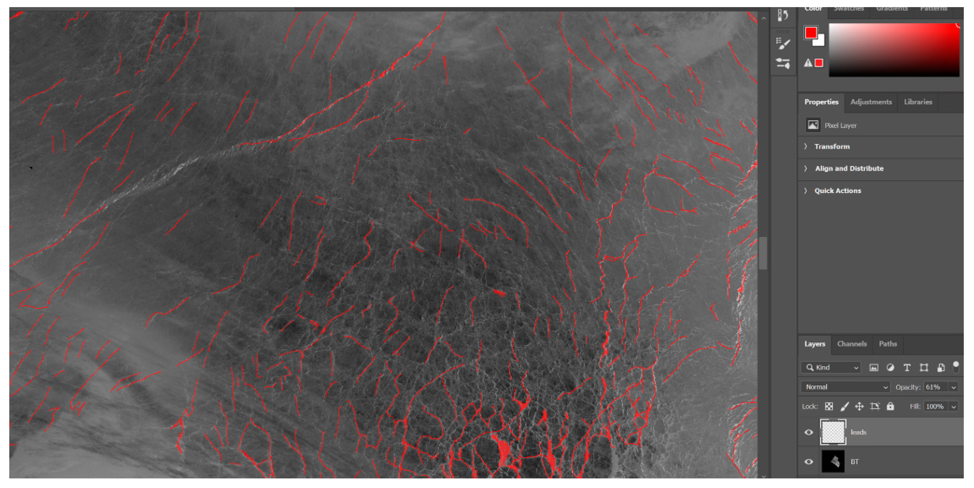
A key to the detection method is the development of a “derived truth” mask and training data set. Because of the remoteness of the arctic, ground truth is not readily available. Hand analysis of satellite imagery serves as the best available option for validation. An example of the hand analysis workflow is depicted in Figure 1. A leads mask (red) is an image layer drawn on top of a 11 µm brightness temperature image where leads are identified using a stylus and touch screen in image editing software. The leads mask layer is exported as a standalone image to be used for training. The “truth” mask and training dataset are developed with an iterative approach. In the first iteration, hand analysis was used to draw a leads mask that was readily apparent in a brightness temperature image. Using this hand analysis, a model was trained and tested. For the subsequent iterations, detection results from the previous model iteration are used as a starting point. Image editing software again is used; an eraser tool manually deletes obvious commission errors and drawing tools add obvious omission errors. The masks do not need to be perfect; the detection model is functional even if the training dataset included omission and commission errors. Results improve with each iteration; fewer errors are apparent and less hand analysis is necessary to edit the truth masks as the detection skill increases. Ultimately, a test case dataset with “truth” masks was developed for four days, 1 January, 1 February, 1 March, and 1 April all from 2020. The lead masks are used as a proxy for “ground truth”, representative of leads that are large enough to be readily apparent in both MODIS and VIIRS.

A particular type of convolutional neural network, a U-Net, was originally described in the literature [19] for the field of microbiology as a way to detect cell walls in microscopic imagery. Despite the vastly different physical properties and scales, the U-Net application in microbiology example in Figure 2 of Ronneberger et al. [19] is visually similar to the U-Net model detection of sea ice leads using satellite imagery example illustrated in Figure 2 of this study. A version of U-Net code, as available in an online code repository [17], has been applied to detect sea ice leads using the 11 µm brightness temperature imagery from MODIS (band 31, AQUA and TERRA imagery, with corresponding geolocation data [20,21,22,23] and VIIRS (I-5, SNPP and NOAA-20 imagery and navigation [24,25,26,27] north of 60° latitude. A description of the parameters used in the sea ice leads detection U-Net model is described in

Table 1. Parameters used in U-Net.

Parameter	Value
Activation—inner layers	Relu
Activation—last layer	Sigmoid
Loss function	Binary cross-entropy
Optimizer	Adam
Learning rate	0.0001
Number of epochs	200
Steps per epoch	30
Batch size	2

; a more complete description of the model is available in Ronneberger et al. [19] and on GitHub [17].

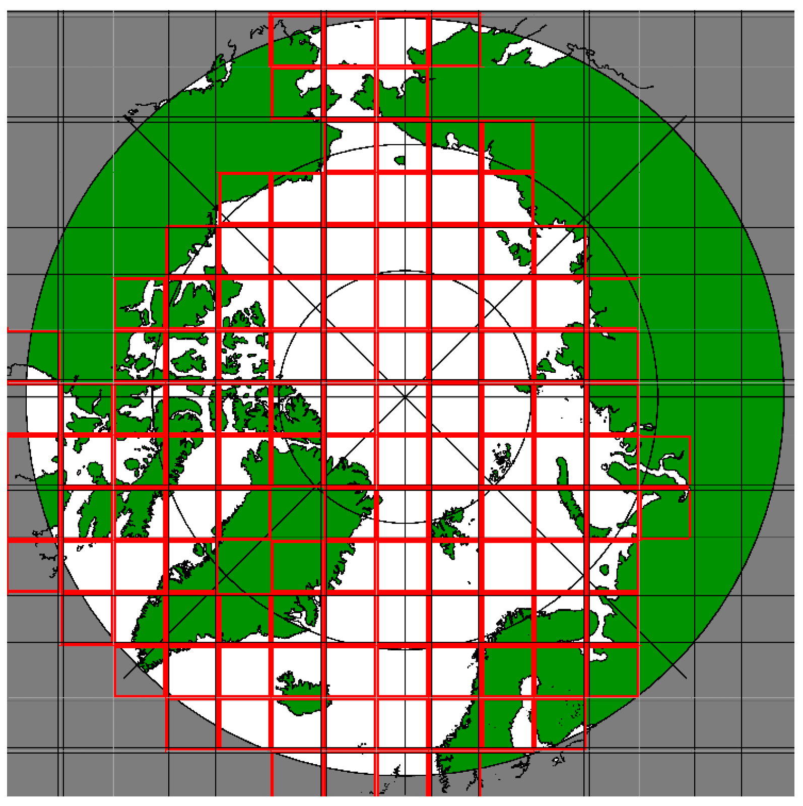
The U-Net [17] was developed to work for 512 × 512 pixel imagery. For the application of lead detection, satellite imagery is remapped to an equal area, 1-km resolution EASE-Grid 2.0 [18] and then divided into 512 × 512 pixel tiles. For testing, the projected imagery from each satellite granule is divided into tiles as shown in Figure 3. The tiles are spaced with 50 pixels of overlap, and the results from the outermost 25 pixel boundary are ignored to avoid detection artifacts around the tile edges. Sea ice lead detection is attempted for each tile containing imagery over ocean water, and the resulting tiles are then reassembled to form a detection mask for each satellite granule.

For training, 6000 lead mask (label) tiles are generated from the derived-truth masks along with tiles of the corresponding satellite imagery from MODIS and VIIRS on three of the four day case study. To separate testing and training, separate input imagery is used. The models train using brightness imagery averaged over 3-h time-series (multiple satellite overpasses occur over each 3-h period and temperature imagery is averaged at these locations), while the test dataset includes individual granule imagery (no time-averaging). The training imagery spans the polar domain (the domain is on the order of 7000 × 7000 km, but individual imagery granules only occupy a small proportion of the domain) and is much larger than the 512 × 512 km/pixel U-Net model domain. To augment the training data, rather than following the tile pattern shown in Figure 3, (used when testing the model), training image tiles are randomly positioned within the much larger polar domain. In this way, an order of magnitude more samples (512 × 512 km images) can be generated for training than testing. The same area may appear in multiple training images, but the amount of overlap is random such that lead features do not appear at the exact same position in the training dataset, and the samples positions will be different from those used in testing. 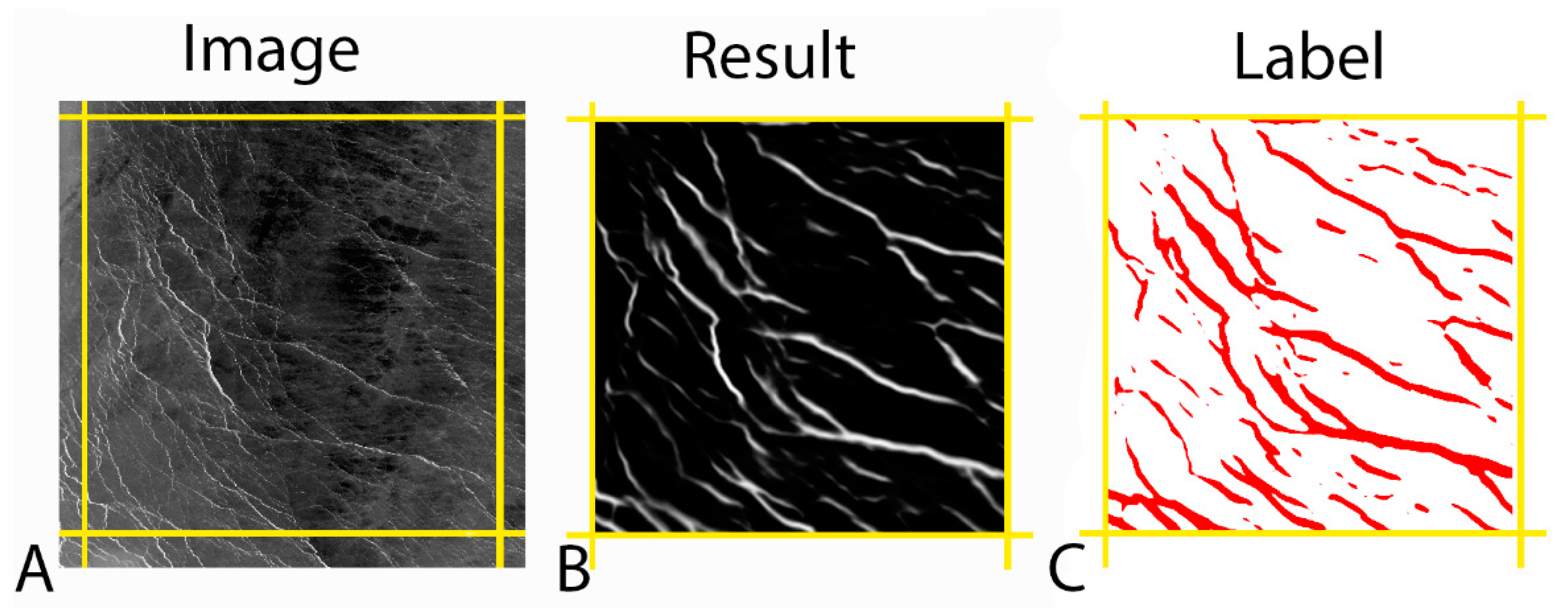To further separate training and testing data—and to avoid overfitting—previously established data augmentation methods are applied to the training data [17]: rotation, width shift, height shift, shear, zoom, and horizontal flip. To avoid edge artifacts, a small buffer region of 50 pixels is used so that there is some overlap in the coverage tiles but the 25 pixels along the edge are discarded (as depicted in yellow in Figure 2).

The above method was used to train two models in TensorFlow 2.2.0. One model trained exclusively with MODIS data, the other with VIIRS data. Each model was trained with 6000 tiles (512 × 512 pixels): 30 images per step times 200 epochs. As previously developed [19], loss was calculated with the TensorFlow binary crossentropy loss function. The U-Net technique used was previously developed [19] and coded in Python [17]; the intention of this project is only to apply largely off-the-shelf software for a new application—sea ice leads detection.

Each tile is processed by the U-Net, creating a per-pixel lead prediction array of values in the range 0–1. That lead prediction array is scaled and interpreted as an 8-bit image, read as a byte array of U-Net detection score values with pixel brightness ranging from 0 to 255 (as shown in Figure 2B). Each pixel in the scaled leads prediction image is classified as lead or non-lead based on a detection threshold; lead prediction pixels brighter than the threshold are classified as leads (as shown in Figure 2C). 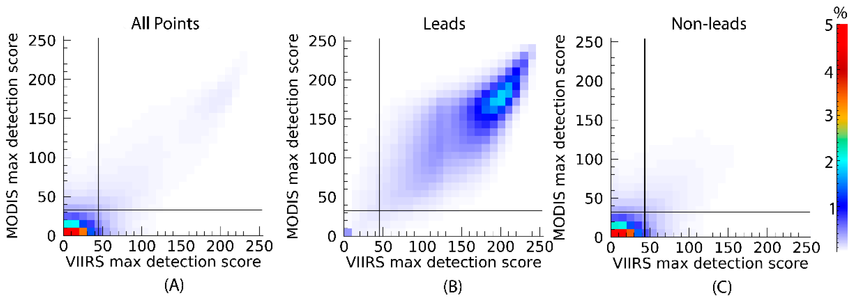Illustrated in Figure 4, the distribution of detection scores overall is bimodal in Figure 4A. In the “Leads” panel, Figure 4B, the majority of lead scores are well above the detection thresholds. 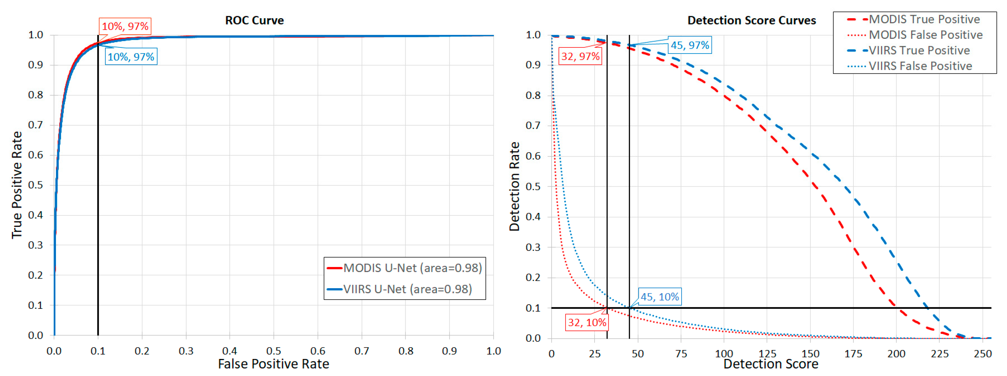Conversely, lead-free locations are depicted in the “Non-Leads” panel, Figure 4C, to illustrate that non-lead detection scores tend to be near zero. The detection thresholds are based on the receiver operating characteristics (ROC) plot in Figure 5. The detection thresholds are defined for each satellite as the ROC curve intersection with the 10% false positive rate line, which is illustrated on the left of Figure 5. On the right of Figure 4, the corresponding false positive and true positive rates are shown as a function of the maximum daily detection score. Here the false positive rate is defined as the false positives divided by the total number of negatives and the true positive rate is the number of true positives divided by the total number of positives. With the detection thresholds at the intersection of the false positive curve with the 10% line, the corresponding MODIS detection threshold is 32/255 and the VIIRS detection threshold is 45/255 (both with a 97% true positive rate).

The detection process is repeated for each overpass. After all granules are processed, daily composite results are recorded in the corresponding MODIS or VIIRS product file that contains an array with the number of total overpasses, the number of overpasses with a potential lead detection score above the detection threshold, and the maximum detection score at each location. A pixel is considered a positively identified sea ice lead if the U-Net lead detection score is above the threshold in three or more overpasses. While the detection threshold for a potential lead was defined as having a false positive rate of 10% (as illustrated in Figure 4), by using repeat detection criteria, the false positive rate for positively identified leads is reduced by approximately 50%. Validation is performed by comparison of the daily composite results against the hand-derived validation masks.

3. Results

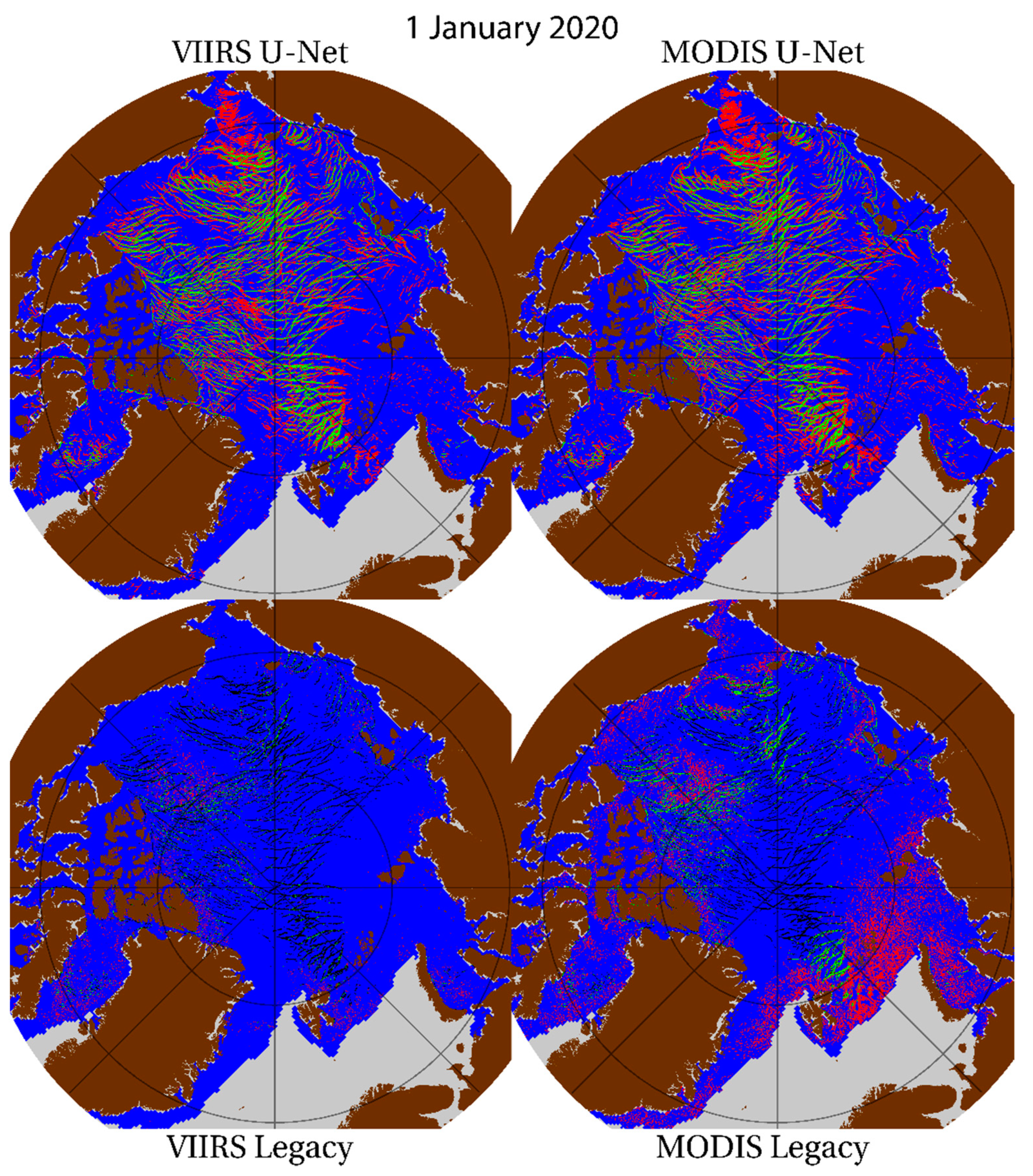
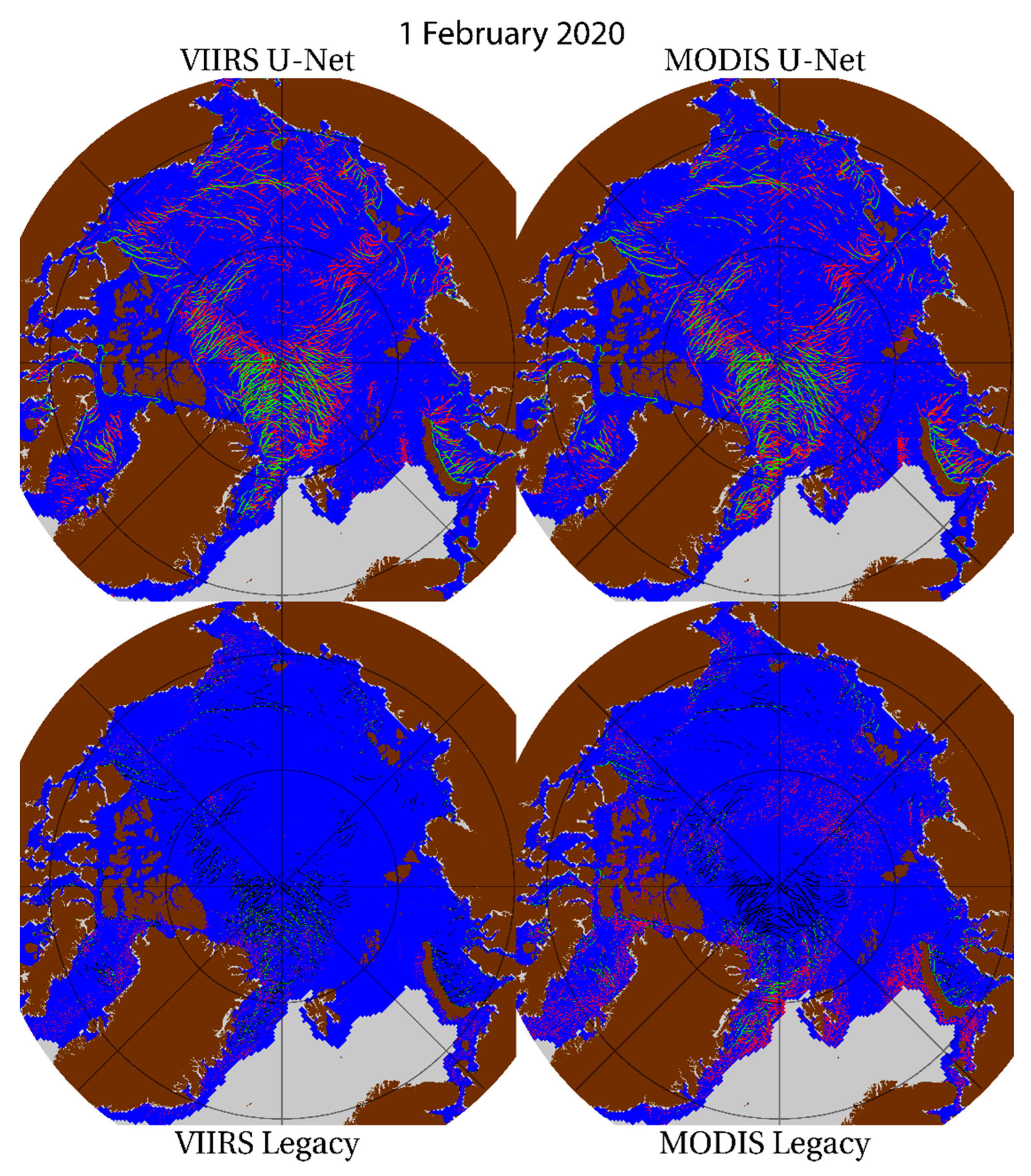
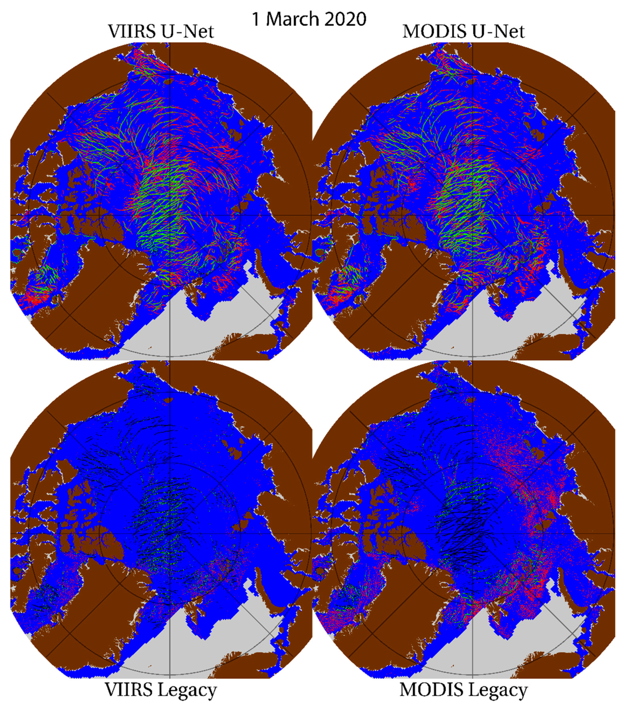
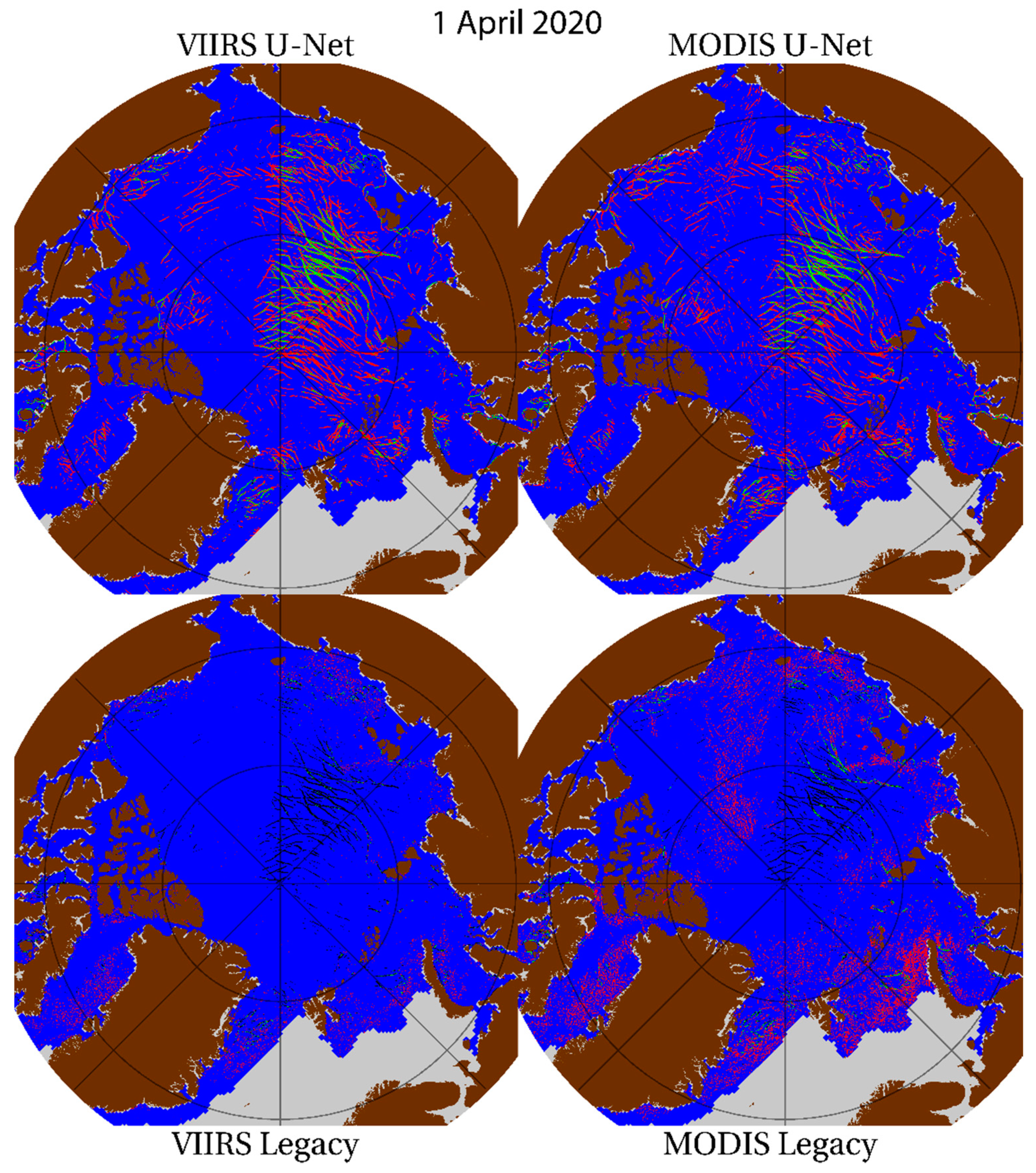
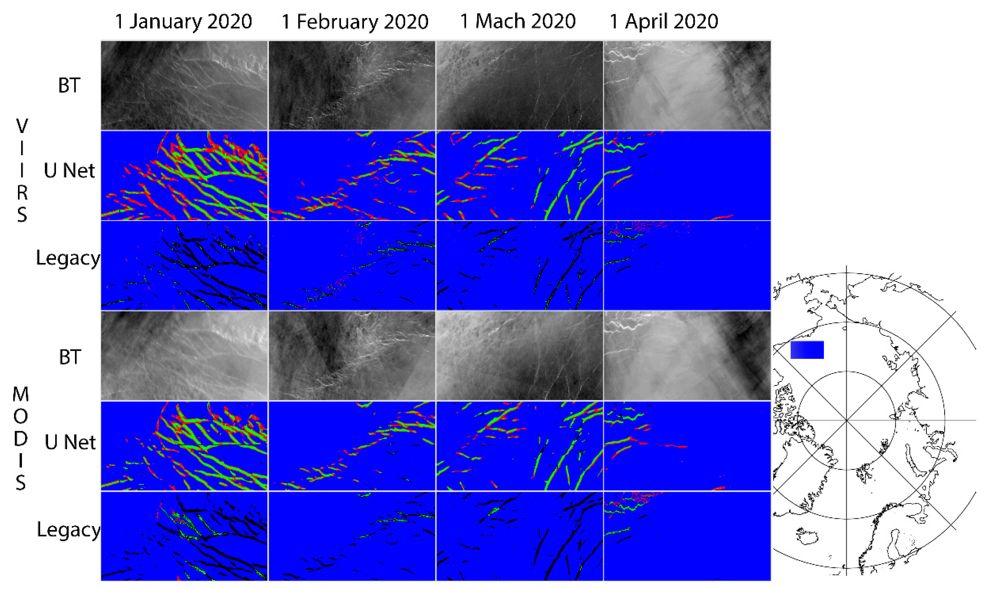
Results from the Beaufort Sea on the first day of January, February, March, and April, 2020 are shown in the multi-panel image in Figure 6 (results from the entire domain are available in the Appendix A). In this region and for the Arctic in general, the overwhelming majority of cases are true negatives or “correct negative” (blue), where validation and detection both identify as not a lead. True positives or “hits” (green) are where the validation mask and detection technique identify a lead; a false positive or “false alarm” (red) is where a lead is detected despite the absence of a lead in the validation mask. A false negative or “miss” (black) is where the validation mask contains a lead that is undetected by the given detection technique. Again, in the absence of ground truth in the Arctic, the masks derived from hand analysis are used as a proxy for validation. There are more true positives (or hits, green) with the U-Net than the legacy product. The legacy product is prone to false negatives (or misses, in black). Through visual inspection of the region shown in Figure 6 and the rest of the Arctic shown in Appendix A, there is significantly more agreement in terms of co-located detections between MODIS and VIIRS when comparing the U-Net products, in contrast to the legacy technique, which does not show strong agreement across satellite platforms. For the April case (far right), persistent cloud cover significantly reduces the amount of detectable leads in the Beaufort Sea. In the other cases, there appears to be some evidence of intermittent cloud contamination, but the U-Net is largely able to detect leads in partly cloudy conditions. In contrast, the legacy lead detection algorithm has a cloud mask dependency, which prevents lead detection in regions flagged as cloudy, and this is a factor in the under-detection of leads in the legacy product.

To avoid errant lead detections in open water, a post-processing step is used to filter the results by a mask of sea ice concentration [28] so that sea ice leads are only considered within the largest expanse of continuous sea ice within the Arctic Ocean. The resulting statistics are given in

Table 3. Lead detection statistics for the aggregate results from 1 January 2020, 1 February 2020, 1 March 2020, and 1 April 2020. The percent correct (PC), probability of detection (POD), false alarm ratio (FAR), critical success index (CSI), Hanssen-Kiuper skill score (KSS), and F1 Score are provided with defining equations for variables defined in Table 2. Results are reported for positively identified leads with potential leads in parentheses.

	PC $\frac{\mathit{A}+\mathit{D}}{\mathit{A}+\mathit{B}+\mathit{C}+\mathit{D}}$	POD $\frac{\mathit{A}}{\mathit{A}+\mathit{C}}$	FAR $\frac{\mathit{B}}{\mathit{A}+\mathit{B}}$	CSI $\frac{\mathit{A}}{\mathit{A}+\mathit{B}+\mathit{C}}$	KSS $\frac{\mathit{A}\mathit{D}-\mathit{B}\mathit{D}}{\left(\mathit{A}+\mathit{C}\right)\left(\mathit{B}+\mathit{D}\right)}$	F1 Score $\frac{\mathit{A}}{\mathit{A}+0.5\left(\mathit{B}+\mathit{C}\right)}$
VIIRS: Positive U-Net (Potential)	94% (88%)	93% (97%)	0.50 (0.68)	0.48 (0.32)	0.88 (0.85)	0.65 (0.48)
MODIS: Positive U-Net (Potential)	95% (88%)	92% (97%)	0.46 (0.68)	0.51 (0.32)	0.88 (0.85)	0.68 (0.48)
VIIRS: Legacy (Potential)	94% (93%)	15% (18%)	0.63 (0.67)	0.12 (0.13)	0.14 (0.15)	0.22 (0.23)
MODIS: Legacy (Potential)	94% (88%)	16% (30%)	0.66 (0.82)	0.12 (0.13)	0.14 (0.22)	0.22 (0.23)

. Because of the imbalanced nature of lead distributions—the proportion of correct predictions (PC) is largely an artifact of the prevalence of true negatives, and not necessarily an indication of detection skill. The more pertinent detection metrics are reported and defined in Table 3, the probability of detection (POD, which is also known as Recall), False alarm ratio (FAR), critical success index (CSI, which also known as Intersection over Union or IoU), Hanssen-Kuiper skill score (KSS), and F1 Score.

Table 2. Contingency table, color coded legend for Figure 6 and variable codes for Table 3.

	Validation Mask Lead	Validation Mask Non-Lead (Sea Ice)
Product lead	A (True Positive, “hit”)	B (False Positive, “false alarm”)
Product non-lead (sea ice)	C (False Negative, “miss”)	D (True Negative, “correct negative”)

defines these metrics and reports the results for positively identified leads and potential leads. The F1 Score is calculated as 2 × ((precision × recall)/(precision + recall)). It is also known as the F Score or F Measure. Precision is the number of true positives divided by the sum of true positives plus false positives, and recall or POD is the number of true positives divided by the sum of true positives plus false negatives. For completeness, a full suite of statistics is provided, however the F1 Score and CSI (or IoU) are the most significant statistics for this application because both give weight to true positives, false positives, and false negatives, without giving weight to the most common true negative category.

The detection criteria are different between the legacy and U-Net approach, but the general concept between a potential lead and positively identified lead is similar. 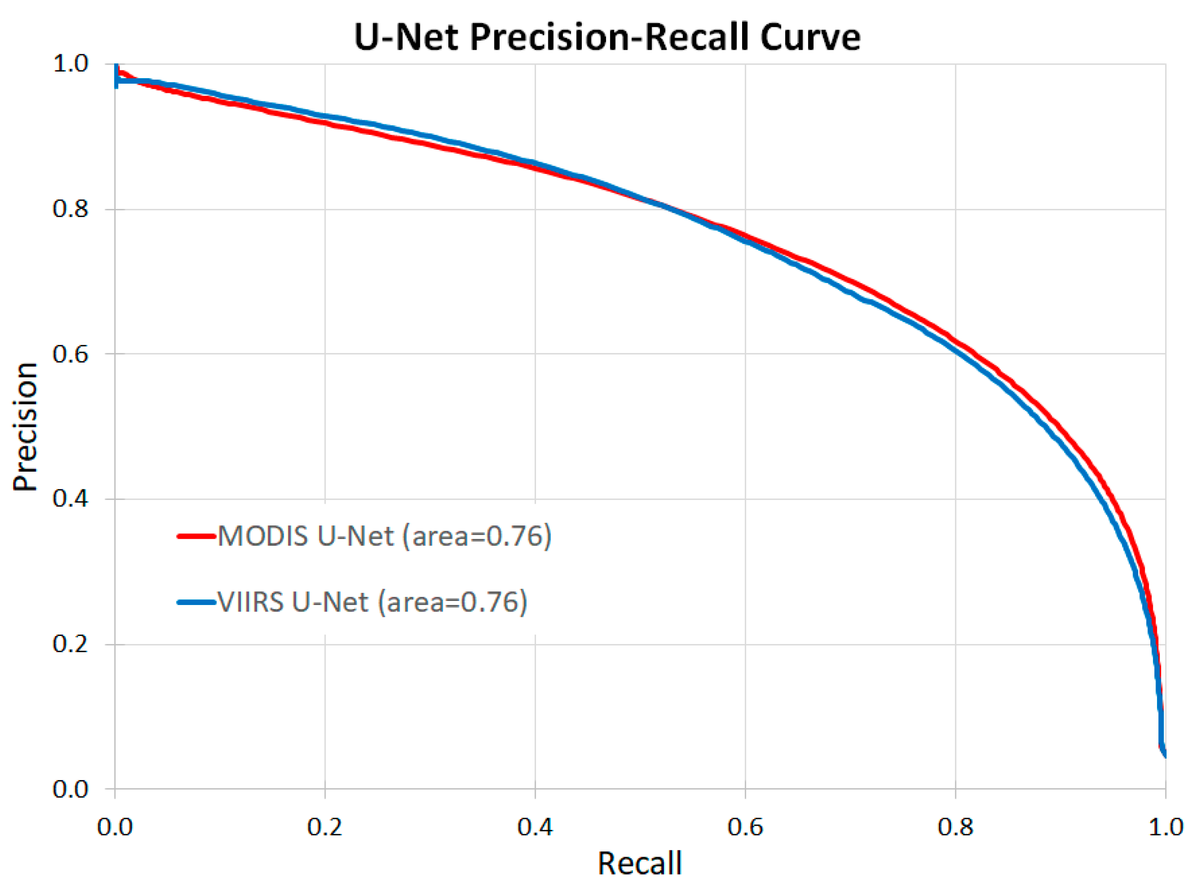In the legacy algorithm, a potential lead is defined as any area with thermal characteristics of a lead (primarily high thermal contrast relative to surrounding pixels), and a positively identified lead is the subset of potential leads that pass a series of conventional tests (Sobel, Hough, etc.,) [11]. For the U-Net leads, a potential lead is any location with a U-Net score above the detection threshold, while a positively identified lead is in the subset of potential lead where the detection occurred in three or more overpasses within the same day. Depending on the end user’s application—sensitivity to omission or commission errors, potential leads generally maximize the true positives while positively identified leads minimize the false positives. As a result, potential leads tend to have higher POD and KSS scores, but positively identified leads have higher PC, CSI (IoU), FAR, and F1 scores. In comparison to the legacy technique, the U-Net technique has on the order of six times the POD and four times the skill scores (CSI, KSS, and F1), while also showing a small reduction in false detections (FAR). It is also significant to highlight the skill improvement attained through the repeat detection criteria used to elevate a potential lead to a positively identified lead. The F1 Score for a U-Net positively identified lead shows more skill compared against a potential lead, whereas there is no F1 Score improvement between potential and positively identified leads in the legacy technique. Another measure of detection skill is illustrated in the precision recall curves in Figure 7 where both MODIS and VIIRS demonstrate significant detection skill with nearly identical curves and area under the curve equal to 0.76.

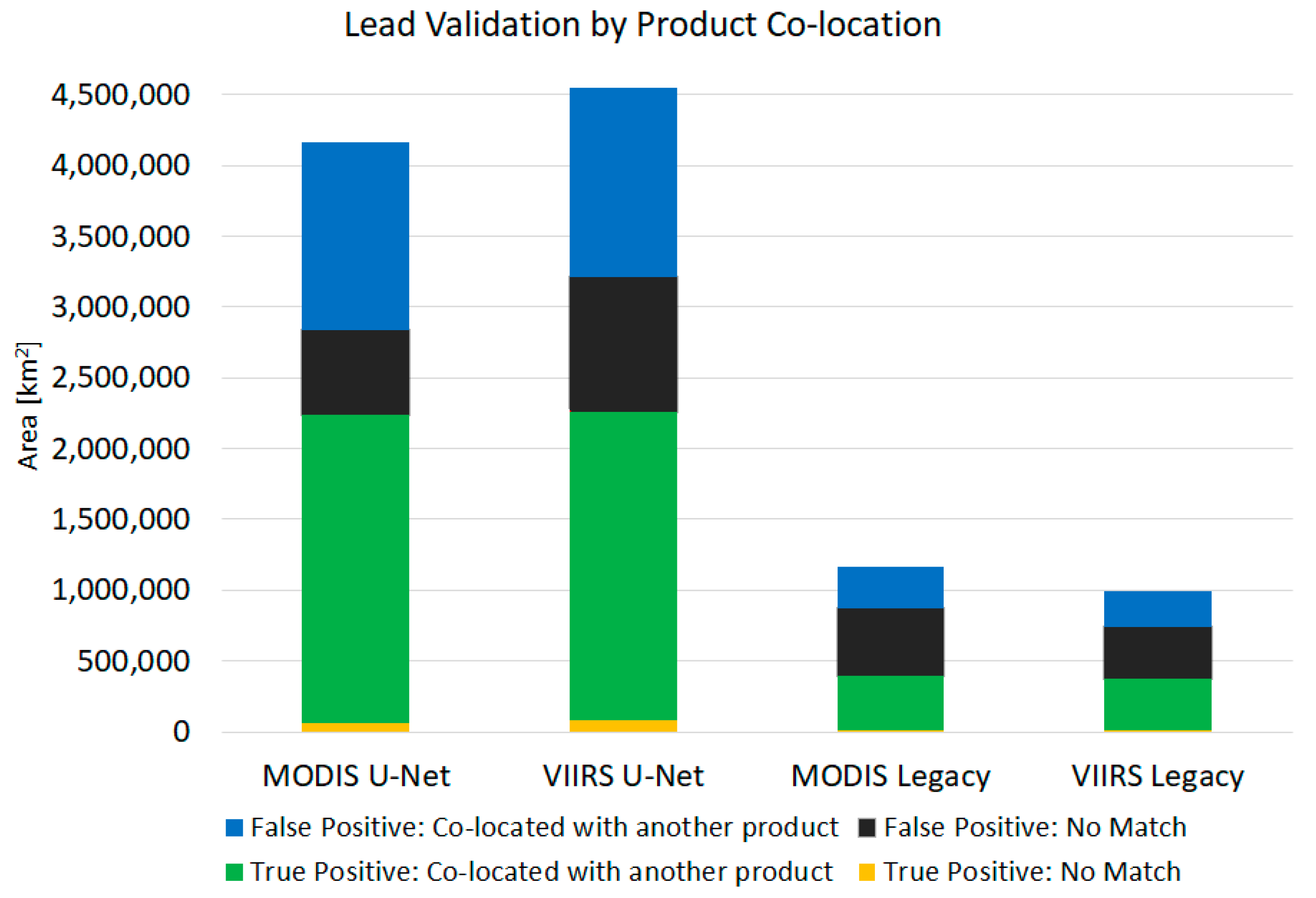
Not only does the U-Net technique show significant improvement in detection skill, one of the primary motivations to develop a new sea ice leads detection technique was to achieve better cross-satellite product agreement than was being achieved with the legacy product. There should be wide agreement between both satellites; only minor differences between satellites would be attributed to differences in overpass time, spatial resolution, and to a lesser degree, scan angle and spectral differences. An analysis of the co-location of detections is shown in Figure 8. Again, the aggregate of lead detections by satellite and detection method from 1 January 2020, 1 February 2020, 1 March 2020, and 1 April 2020, are grouped based on if the lead detection corresponds with another lead detection and/or with a lead in the validation mask. The majority of the U-Net detections are co-located with a valid lead (green and blue). In contrast, a larger proportion of the leads in the legacy product are not co-located with another product detection (black). Among the detections that are not co-located with another product detection, we would suspect that leads detected by multiple products but not the validation mask (blue) are most likely an artifact of an imperfect validation mask (omissions in the validation mask), which is consistent with a visual inspection of the masks. In contrast, the false positives without a co-located lead detection (black) are more likely a mixture of false detections and omissions from the validation mask. The significance is that the false detections that are in only one product (red) make up a much smaller proportion of the U-Net lead detections than the legacy lead detections. Moreover, visual inspection of the result masks is consistent with this interpretation, where many of the “false” leads detected by U-Net appear to be omission errors in the validation masks, while cloud edge artifacts appear to be the likely cause of the false detections visually apparent in the legacy product. Overall, the U-Net technique is a significant improvement over the legacy technique with more true positives, false positives that tend to look like true leads (likely validation mask omissions), and fewer false negatives.

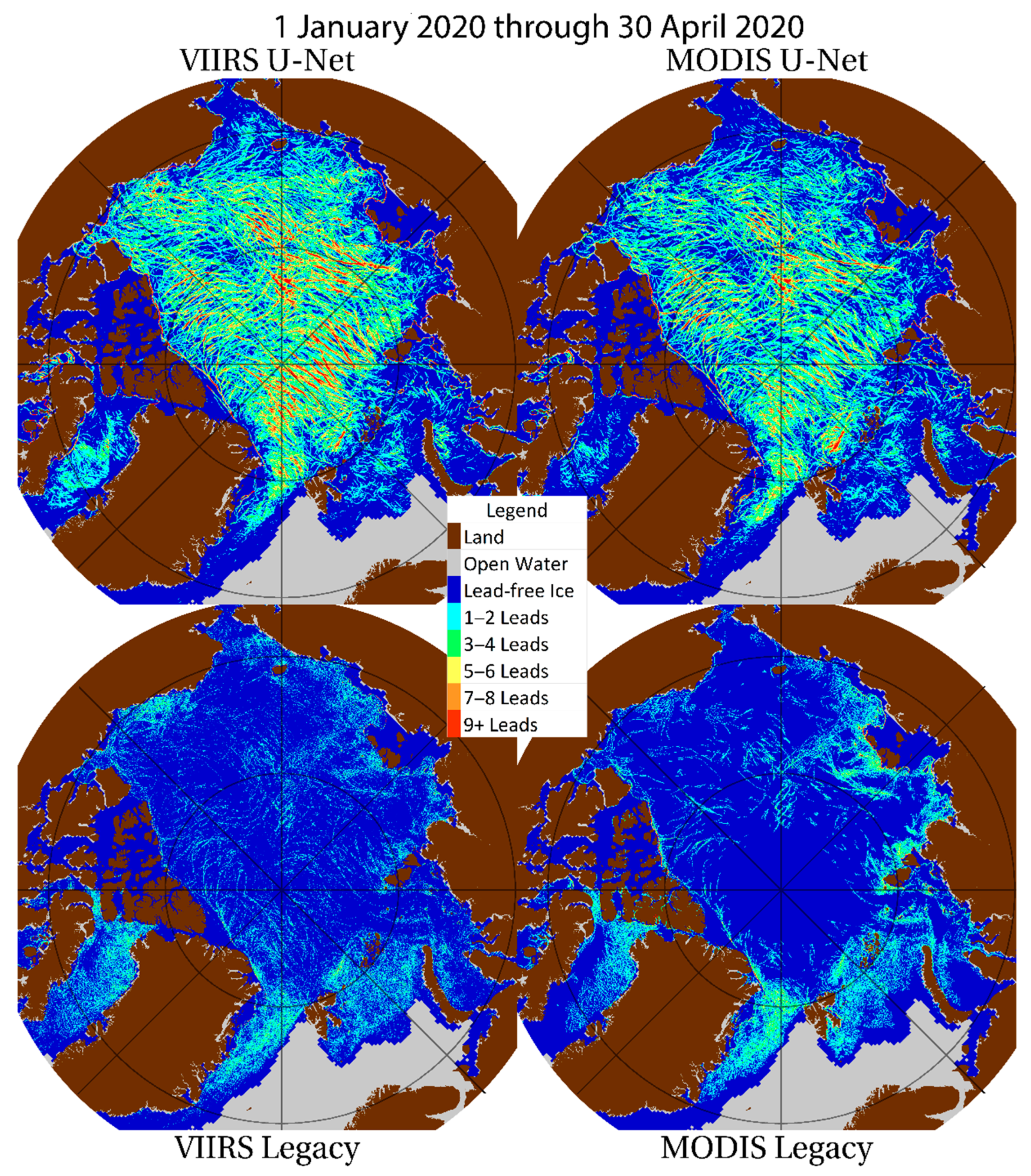
Using a fairly limited dataset with only four days of hand analyzed validation masks, three of the four day validation sets were used to train the model; the remaining day was withheld for testing and validation. The detection performance from the three days within the training dataset are indistinguishable from the fourth day that was withheld from the training dataset. To further ensure results are not overfit to the truth masks, a test case, spanning January through April of 2020 and composite results are illustrated in comparison with the legacy product in Figure 9. Beyond the four-day case study, validation data are limited, so it is not possible to perform the same rigorous detection skill analysis as presented for the cases where hand-analyzed validation masks exist. However, results from the winter of 2020 confirm that the U-Net does provide more consistency between MODIS and VIIRS than in the legacy product. Given the spatial patterns of the aggregate results, we infer that the U-Net appears to have many more true positives (detection features that look like leads) and fewer false positives (fewer small features that look like cloud edge artifacts) than the legacy product. A more rigorous study of lead detection over a long time series will be the focus of upcoming work.

4. Discussion

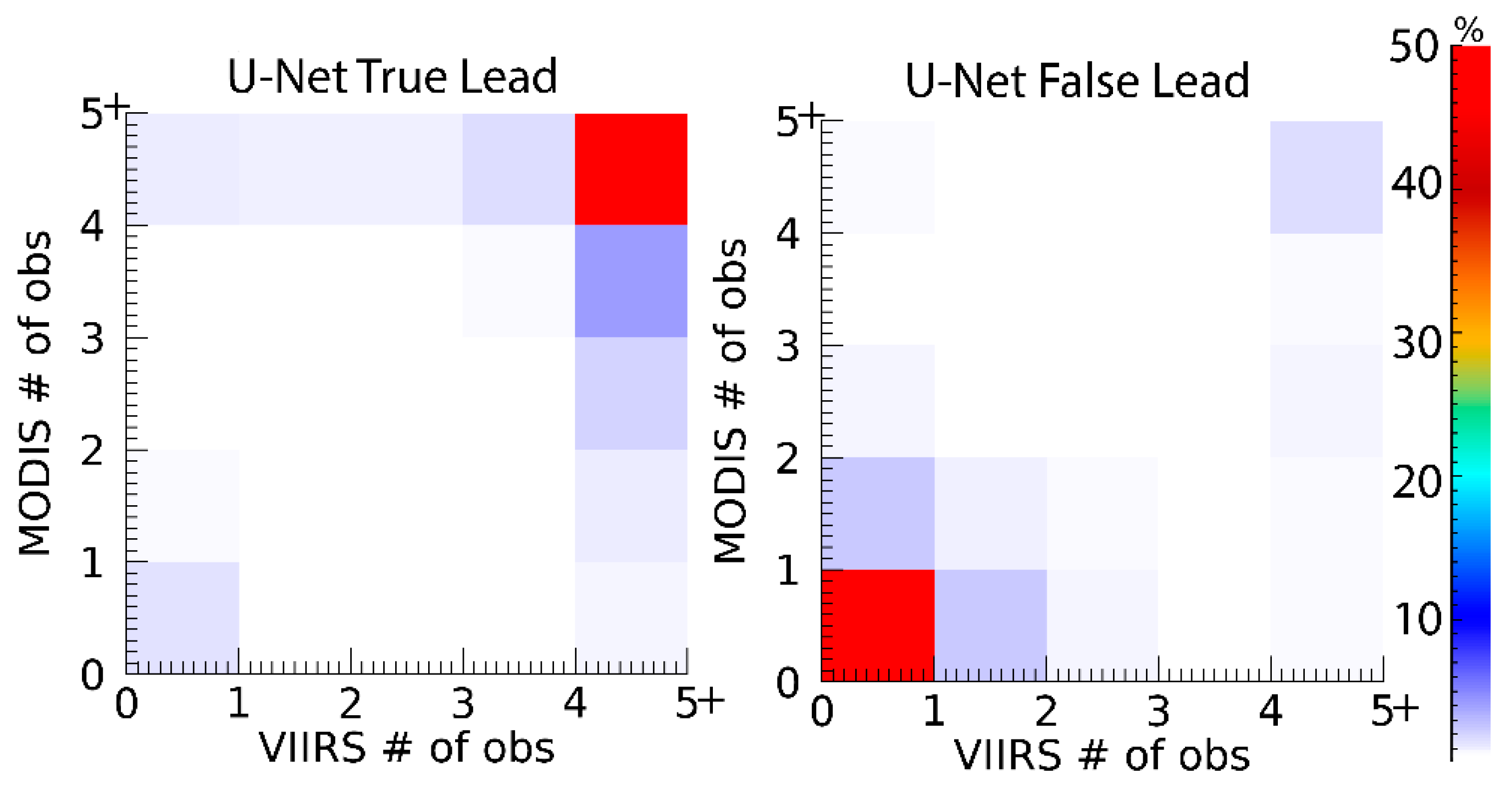
The premise is that the more often a potential lead occurs during the course of a day, the more likely it is that the potential lead is a true lead, whereas fewer repeat observations tend to be related to false positives, for example, short lived features such as a cloud edge. Figure 10 illustrates detection skill inferred by the number of repeat observations of a potential lead. The majority of leads are observed in more than four overpasses, and in the right, non-leads tend to have a lead detection score above the detection threshold in less than three overpasses.

We anticipate that expanding the validation set and retraining the model in future work will likely continue to improve detection metrics. Similarly, future work could retrain the U-Net based on validation datasets from higher resolution instruments such as Synthetic Aperture Radar [29] or Sentinel-2 [30], compared against other products, and/or applied to other historical, current, or future satellite imagery while also exploring other visible, thermal, and microwave bands. As an example, a comparison has been performed of the satellite altimeter based ICESat-2 sea ice leads product [31] against the U-Net and legacy thermal IR-based lead products. Given the very narrow spatial coverage (approximately 10-m beam width) and 91 day coverage cycle from ICESat-2, it would be difficult to derive validation imagery that could be used to train IR-based lead detections. We would expect to see significant differences in the amount of leads that can be detected on different spatial scales, for moderate resolution IR imagers, we would not expect to detect leads narrower than approximately 250 m [32,33,34]. However, it is possible to identify the frequency of an IR-based lead co-located with a detection from the altimeter, and these results are summarized in

Table 4. ICESat-2 co-location with moderate resolution lead detection; aggregate results from 1 January 2020, 1 February 2020, 1 March 2020, and 1 April 2020. Results are reported as the percentage of ICESat-2 leads with a lead detection within 1 km of a MODIS and/or VIIRS lead detection. Positively identified leads are reported first, with potential leads in parentheses.

	U-Net	Legacy
MODIS	19% (27%)	8% (17%)
VIIRS	21% (28%)	7% (8%)
MODIS or VIIRS	23% (32%)	13% (21%)
MODIS and VIIRS	17% (23%)	2% (5%)

. Again, given the spatial resolution of the ICESat-2 ATLAS laser measurements are two orders of magnitude smaller than the 1-km resolution of the IR leads product, we would expect a significant proportion of sea ice leads detected by ICESat-2 will be too small for detection with moderate resolution IR. However, what can be observed in the comparisons against ICESat-2 is that the U-Net technique detects more leads than the legacy technique. Moreover, with the U-Net there is significantly better agreement between MODIS and VIIRS; only a small proportion of U-Net lead detections are detected by one but not both satellites, whereas the legacy product shows relatively poor agreement between satellites. Overall, the comparisons with ICESat-2 are consistent with the findings from the IR-based validation masks. At present the U-Net preforms well detecting moderate to large-scale leads; further research would be necessary to detect small scale, sub-resolution leads. For example, sub-resolution leads would be more readily detected using a 4–11 µm brightness temperature difference.

Some differences will be expected across satellite platforms due to differences in orbital patterns (overpass times) where leads may move or change, clouds may obscure the leads, etc. Further, due to spatial differences in the instruments, we would expect the coarser resolution MODIS data to have a bias toward detecting wider leads while VIIRS, with finer resolution, would detect narrower leads that may be too small to have a detectable signal in MODIS. Comparing the MODIS and VIIRS detection score densities illustrated in Figure 4, there is a slight bias where the VIIRS score tends to be slightly higher than MODIS, and this is also reflected in the slightly different detection thresholds.

5. Conclusions

The nature of AI is that the quality of the results are limited by the quality of the training datasets. In the application presented here — detecting sea ice leads (fractures) in satellite imagery —developing quality validation may be the limiting factor due to the laborious and imperfect hand analysis. However, in some ways the qualitative detection skill may exceed quantitative detection skill; i.e., visual inspection of the results shows that valid leads are detected in areas that the validation mask flags as lead-free. As work progresses, adding more cases to the validation set should help minimize omission and commission errors. Going forward, comparisons against time-matched imagery from higher resolution imagery or lead masks from other sources could also be a good way to validate results. However, using the existing validation dataset has shown that the U-Net architecture can successfully be applied for the detection of sea ice leads from moderate resolution satellite-based thermal imagery. Results demonstrate a high level of detection skill, and improvement of the legacy technique, with more true positives, few false positives, fewer false negatives, and better agreement between satellite instruments.

Ultimately, work will continue toward the application of this U-Net technique to the entire MODIS and VIIRS time-series. From this archive, in excess of 20 years, a rigorous analysis of the characteristics of sea ice leads will be studied. By establishing separate models for MODIS and VIIRS, the intention is to be able to provide a stable leads product over the entire satellite archive. As MODIS nears end of life, the VIIRS product will be able to continue to provide leads detection products for years to come. Furthermore, the initial work has been focused on the detection of leads in the winter season; it may be necessary to expand the training dataset to include warm season cases (that include warm season clouds and melt ponds) before the technique could be applied to the summer season.