Abstract
NASA’s ICESat-2 has been providing sea ice freeboard measurements across the polar regions since October 2018. In spite of the outstanding spatial resolution and precision of ICESat-2, the spatial sparsity of the data can be a critical issue for sea ice monitoring. This study employs a geostatistical approach (i.e., ordinary kriging) to characterize the spatial autocorrelation of the ICESat-2 freeboard measurements (ATL10) to estimate weekly freeboard variations in 2019 for the entire Ross Sea area, including where ICESat-2 tracks are not directly available. Three variogram models (exponential, Gaussian, and spherical) are compared in this study. According to the cross-validation results, the kriging-estimated freeboards show correlation coefficients of 0.56–0.57, root mean square error (RMSE) of ~0.12 m, and mean absolute error (MAE) of ~0.07 m with the actual ATL10 freeboard measurements. In addition, the estimated errors of the kriging interpolation are low in autumn and high in winter to spring, and low in southern regions and high in northern regions of the Ross Sea. The effective ranges of the variograms are 5–10 km and the results from the three variogram models do not show significant differences with each other. The southwest (SW) sector of the Ross Sea shows low and consistent freeboard over the entire year because of the frequent opening of wide polynya areas generating new ice in this sector. However, the southeast (SE) sector shows large variations in freeboard, which demonstrates the advection of thick multiyear ice from the Amundsen Sea into the Ross Sea. Thus, this kriging-based interpolation of ICESat-2 freeboard can be used in the future to estimate accurate sea ice production over the Ross Sea by incorporating other remote sensing data.
1. Introduction
Sea ice in the polar regions plays an important role in global climate by interacting with the ocean and atmosphere [1]. Snow-covered sea ice reflects a significant amount of incoming solar radiation back to space [2,3,4,5], thus working as an insulator between the ocean and atmosphere [6]. The annual variations of sea ice cover can influence ocean and atmospheric circulation [7,8], surface temperature [9], and ecology [10,11]. According to previous studies, sea ice extent and thickness in the Arctic has decreased since the 1960–1970s, mainly due to the dramatic increase in atmospheric CO2 emissions and its associated warming, which has a stronger signature in high northern latitudes [4,12,13,14,15,16]. In contrast with the Arctic, several Antarctic studies have reported that sea ice extent increased for last 40 years, but started to decrease dramatically after a record high in 2014 [17,18]. Sea ice thickness and volume have also slightly increased, but a definitive trend is not available [19,20].
In particular, the Ross Sea is one of the most noticeable regions showing a significant increase of sea ice extent in the Southern Ocean [17,21,22]. There, massive amounts of sea ice are produced in the Ross Sea polynya which is the largest recurring polynya area in Antarctica [23,24,25]. Thus, sea ice dynamics in the Ross Sea has been the subject of a number of scientific studies [1,26,27,28,29,30]. Due to the harsh weather and long polar nights, spaceborne remote sensing has been the most common and efficient approach for these studies; spaceborne remote sensing allows obtaining sea ice observations over a large area with regular time spans without the need of physical visits to the study region.
In recent years, the National Aeronautics and Space Administration (NASA)’s Ice, Cloud, and land Elevation Satellite-2 (ICESat-2) has been providing precise sea ice freeboard and thickness estimates over the polar regions. ICESat-2 was launched in September 2018 with the objectives of measuring changes in ice sheets, glaciers, and sea ice thickness [31]. The Advanced Topographic Laser Altimeter System (ATLAS) on ICESat-2 measures the surface heights by using 532 nm wavelength laser photons. ATLAS has six beams of three pairs of strong and weak beams with 11 m footprints spaced by 0.7 m [32], providing a better spatial resolution compared to the previous ICESat mission [33]. Various studies have utilized ICESat-2 for the characterization of sea ice freeboard and thickness in the polar regions, taking advantage of this outstanding spatial resolution [34,35,36].
However, despite the good precision and resolution of ICESat-2, the use of ICESat-2 for studying sea ice is substantially limited by the spatial sparsity of the instrument’s measurements (Figure 1). Since ICESat-2 data is collected along tracks, there are large sections of area for which there is no data because they are not under a track. In addition, ICESat-2 cannot measure freeboard in cloudy conditions because the laser photons do not penetrate clouds. Thus, ICESat-2 data have limitations in sampling sea ice elevation over a large area during a short sampling period, such as one or two weeks. Due to this limitation, ICESat-2 has been so far only used to generate monthly sea ice freeboard or thickness maps over the polar regions based on the near-monthly sub-cycle of its orbit [31,35,36,37]. Even though these monthly maps are useful in understanding the overall annual trend of sea ice thickness, they cannot capture short-term formation and dynamics of sea ice, especially in regions where sea ice moves very rapidly, such as near the polynya ice production areas. Since the wind speed and wind direction in the Ross Sea change very rapidly even on a daily scale [38,39,40], the spatial distribution of sea ice freeboard over the Ross Sea can fluctuate significantly in a short period. Thus, weekly maps of the sea ice freeboard over the Ross Sea should provide an improved characterization of sea ice production and drift in the polynya areas when compared to monthly maps.
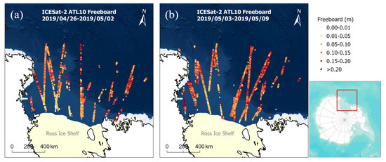
Figure 1.
Actual ICESat-2 ATL10 data coverage in the Ross Sea for the following 1-week periods: (a) 04/26/2019–05/02/2019 and (b) 05/03/2019–05/09/2019. The presence of spatial gaps due to the orbit separations and existence of clouds is readily apparent.
In order to address the spatial sparsity of ICESat-2 and produce weekly freeboard maps over the Ross Sea, we employ a geostatistical kriging approach. Kriging is a popular and well-established spatial interpolation methods for estimating unknown values [41]. In addition, one of the advantages of using kriging is that it is useful to examine the spatial autocorrelation of data (e.g., statistically representative range of ICESat-2 data) [42]. Since a mining engineer, Krige, used statistics to estimate ore reserves [43], geostatistical analysis and the kriging method have been used for the mapping of many environmental fields. In terms of the cryosphere, Herzfeld et al. [44] and Iacozza and Barber [45] characterized the snow depth on sea ice from geostatistical variograms, and Huang et al. [46] estimated the spatial distribution of snow depth by using kriging. Kriging is a common method to interpolate ice shelf thickness [47,48] or ice sheet mass balance [49,50,51]. Lindsay et al. [52] and Kurtz et al. [53] used the ordinary kriging to interpolate sea surface heights for the estimation of sea ice thickness, and Wang and Hou [54] used kriging to determine the spatial distribution of surface temperature in the Antarctic. Herzfeld et al. [55] used variograms for the morphological characterization of ice surface types from glacier-roughness sensor (GRS) data.
Although geostatistics is common for various applications, there have been few attempts to apply this geostatistical kriging to short-term mapping of sea ice freeboard or thickness. In this study, we characterize the spatial autocorrelation of the ICESat-2 freeboard measurements in the Ross Sea and apply kriging interpolation to estimate sea ice freeboards in locations where the ICESat-2 track is not available. Finally, based on this geostatistical approach, we generate weekly freeboard maps and analyze the short-term sea ice variability in the Ross Sea in 2019.
2. Study Area
The area of interest for this study is the Ross Sea, which is the southernmost sea of Antarctica located in a deep embayment of the Southern Ocean between Victoria Land to the west and Marie Byrd Land to the east (Figure 2). To generate the weekly maps, the Ross Sea is subjectively limited to the region 78°S–70°S latitude, and between the Victoria Land/Oates Land coast and the 150°W longitude. In addition, considering the general distribution of polynyas and ocean currents in this region, we divide the entire Ross Sea area into four sub-sectors: northwest (NW), northeast (NE), southwest (SW), and southeast (SE) as shown in Figure 2.

Figure 2.
Map of the Ross Sea showing the four subsectors of interest (northwest—NW, northeast—NE, southwest—SW, and southeast—SE) for this study superimposed on a sea ice concentration (SIC) for October 2019 from the U.S. National Ice Center (NIC) ice chart. The three low SIC areas inside the SW are the three known polynyas: the Ross Ice Shelf Polynya (RISP), Terra Nova Bay Polynya (TNBP), and McMurdo Sound Polynya (MSP).
One of the important characteristics of the Ross Sea is its large polynyas, mostly in the SW sector [23,24]. Polynyas can be defined as isolated areas of open water and thin ice within the ice pack in a polar region [56]. The Ross Sea has three large persistent polynyas (Figure 2): the Ross Ice Shelf polynya (RISP), Terra Nova Bay polynya (TNBP), and McMurdo Sound polynya (MSP) [26,40]. The formation of these polynyas from March to November is largely related to katabatic winds from the Ross Ice Shelf and Victoria Land [57,58].
3. Data
In this study, sea ice freeboard data over the Ross Sea region from the ICESat-2 ATL10 (release 003) were obtained from NASA Earthdata (earthdata.nasa.gov). The time period selected for this study was 1 March to 30 November 2019 which covered one annual ice-growth cycle from the start of the freezing season to the start of the melting season. We note that ICESat-2 data from 26 June 2019 to 9 July 2019 were not available because ATLAS was off during this time in the safe-hold mode.
The ATL10 freeboard product is derived from the sea ice surface heights product (ATL07) which in turn was derived by the aggregation of 150 photons from the ATLAS global geolocated photon data product (ATL03). The surface heights of ATL07 are calculated by assuming a Gaussian distribution of the aggregated 150 photons and the precision of this surface height is known as less than 2 cm for flat surfaces [59]. Based on this surface height , the sea ice freeboard of the ATL10 product is calculated as follows:
where is a sea surface reference height estimated from a collection of sea ice leads within a 10 km segment. Herein, this freeboard represents the total freeboard (i.e., the ice freeboard and snow depth), and freeboard is calculated only for where daily sea ice concentration (SIC) is greater than 15% [60]. In the ATL10 product, sea ice floes and leads are classified by three photon factors: photon rate, photon distribution, and background rate [37]. Since the surface heights are derived from the aggregations of 150 geolocated photons, the spatial resolution (i.e., height segment length of 150 photon aggregations) depends on the surface reflectance or roughness. Generally, the segment lengths are 10–200 m for strong beams, and 40–800 m for weak beams [37]. Because the strong beams have better resolutions than weak beams, only strong beams are used in this study.
4. Methods
4.1. Subsampling of ATL10 Product to 3 km
The purpose of this study is to characterize and estimate the overall distribution of sea ice freeboard over the entire Ross Sea by using ICESat-2 observations and the kriging approach. However, for some sea ice floes, ridged ice or thin ice in leads can distort the global freeboard values for level sea ice (Figure 3a). Thus, the ATL10 freeboard data are first resampled every 3 km to reduce the impacts of sea ice deformation (ridged ice or sea ice leads) on the level ice freeboard values (Figure 3b). Geostatistical approaches can have difficulty predicting these local and linear sea ice deformation features because they are based on the assumption of data stationarity [61].
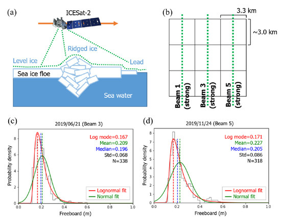
Figure 3.
(a) Diagram of ICESat-2 photon beams over sea ice floes showing that ICESat-2 freeboard measurements include ridges and leads as well as level ice floes, (b) 3 km sampling of ICESat-2 data, (c) distribution of ATL10 freeboard for a single 3 km sample segment on 21 June 2019, and (d) distribution of ATL10 freeboard for a 3 km sample segment on 24 November 2019 (note that the lognormal distribution better fits the real freeboard distributions compared to the normal distribution).
It is known that the sea ice freeboard generally follows a lognormal distribution [62] and the modal freeboard represents the freeboard for level ice [63,64]. Therefore, in order to reduce the effect of the sea ice deformation, the freeboard distributions are fitted to lognormal distributions for every 3 km cell and the modal freeboards for the 3 km cells are considered as representative freeboards of the level sea ice (Figure 3b–d). Since three strong beams of ICESat-2 are separated with 3.3 km intervals, we make the ICESat-2 track data look like ~3 × 3 km2 pseudo-square cells (Figure 3b).
4.2. Geostatistical Modeling
After the ATL10 data are aggregated as modal freeboards every 3 km, we build geostatistical models for interpolating freeboard values to select locations where ICESat-2 observations are not available. A geostatistical model first measures the spatial dependence or autocorrelation from a semivariogram that represents the relationship between the semivariance γ(h) and the lag distance h. The average semivariance at a lag distance h is defined by:
where is the measured sample value (i.e., ATL10 freeboard in this study) at the point , is the measured sample value at another point displaced from the point xi by a lag distance h, and N is the number of observations for a lag distance h.
After an experimental semivariogram is derived from the measurements, the experimental semivariogram must be fitted with a mathematical model to estimate the semivariance at any given distance [42]. This fitted semivariogram has three elements: nugget, effective range, and sill. The nugget (c0) is the semivariance at the distance 0, which means measurement error. The effective range is the distance at which the semivariogram starts to be flat, which means the data have no spatial correlation beyond this range. The sill is the semivariance at this leveling point. Among various types of semivariogram models, three representative variogram models are calculated and compared in this study: exponential, Gaussian, and spherical. These models are defined by the equations:
Based on these variogram models, ordinary kriging is employed to estimate sea ice freeboards. The general equation for estimating the z value at a point is:
where is the estimated value, is the known value at point x, is the weight on the point x, and s is the number of sample points for estimation. The weights are derived from solving a set of simultaneous equations [42]. In this study, Esri’s ArcGIS software is used for the derivation of semivariogram models and ordinary kriging.
In order to cross-validate these kriging models, we divide the weekly data into a training dataset and validation dataset. For every week, we randomly select two tracks as a validation dataset and build kriging models using the other available tracks (Figure 4). This model is then compared to the validation dataset to check if this geostatistical approach is reliable for the estimation of the unknown values. In this process, we compare the three different variogram models to determine which model is the most accurate. After the accuracy of the geostatistical model is assessed, we map sea ice freeboard over the Ross Sea weekly. These freeboard maps have a grid size of 25 km which is comparable to previous sea ice mapping results [35,36,65] and the ICESat-2 Level 3 product of monthly gridded sea ice freeboard (ATL20) [60]. The freeboard for the center of each 25 km grid cell is estimated by applying kriging with the 3 km mode sampled ATL10 data. We note that the mapped freeboard in this study is the total freeboard for level sea ice because the impacts of sea ice deformation (i.e., ridges and leads) are minimized by the previous 3 km mode sampling (Section 4.1). The number of ATL10 tracks used for each weekly map is generally 15–25; the number of used tracks depends on the time and location of ground tracks and cloud cover.

Figure 4.
Flowchart of the geostatistical kriging modelling and mapping.
5. Results
5.1. Cross Validation of Kriging Estimated Freeboards
Figure 5 describes the cross-validation results by time. In general, the correlation coefficient (R) is greater than 0.4, which indicates a moderate correlation [66]. R value is relatively greater in the thicker-ice season from July to November (R > 0.5), but it is relatively low in the thinner-ice season from March to June (R ~ 0.4–0.6) (Figure 5a). Similarly, while the root mean square error (RMSE) and mean absolute error (MAE) are relatively low in March to June, they are relatively high in July to November (Figure 5b,c). The higher errors in July to November may be attributed to higher freeboard values (i.e., thicker ice) during these months.
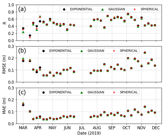
Figure 5.
Temporal variations of cross validation parameters: (a) correlation coefficient (R), (b) root mean square error (RMSE), and (c) mean absolute error (MAE).
The overall cross-validation results of the kriging freeboard estimation for three variogram models are depicted in Figure 6. The exponential, Gaussian, and spherical variogram models show similar results to each other: an R of 0.56–0.57, RMSE of ~0.12 m, MAE of 0.07 m. Although this level of R value indicates only moderate correlation between kriged freeboard and actual freeboard, the p-value (< 0.001) shows that this correlation is significant. Additionally, this cross-validation result implies that the geostatistical approach interpolates and estimates of freeboards in the Ross Sea with an expected RMSE of approximately 0.12 m, and the differences between the three variograms are negligible.
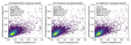
Figure 6.
Scatter plot comparisons of the cross-validation for the three variogram models: (a) exponential, (b) Gaussian, and (c) spherical.
Furthermore, we compare the cross-validation parameters for each subsector: NW, SW, NE, and SE (Figure 7). As shown in Figure 7a, the SW and SE sectors show higher R values than the NW and NE sectors. This is because the ICESat-2 tracks are more densely distributed in the southern regions (Figure 1), which consequently guarantees higher reliability of kriging interpolation for the southern sectors. However, since the RMSE and MAE depend on the freeboard value as well, the SE sector, where the thickest ice is located, shows a higher RMSE and MAE compared to the other sectors (Figure 7b,c). The SW sector generally shows the lowest RMSE and MAE among the four sectors, which should be attributed lower freeboard of the SW sector due to the existence of large polynyas there. More details about ice freeboard and thickness for these sectors and the reason for it are discussed in the following sections.

Figure 7.
Temporal variations of cross-validation parameters for each geographical subsector (NW, SW, NE, and SE): (a) R, (b) RMSE, and (c) MAE.
5.2. Variations of Variogram Factors
We also compare the temporal variations of the variogram factors (i.e., range and sill). As shown in Figure 8a, the effective ranges of the variograms generally range in 5–10 km, but the exponential variogram model shows greater range than the other variogram models because of its mathematical approach (Equation (3)). The exponential model takes a longer distance to reach the level sill points than the other models due to the mathematical characteristics, even though they have all the same experimental semivariograms. Since the ranges of the variograms represent the spatially autocorrelated distance, it can be said that the ICESat-2 ATL10 freeboards are representative of freeboards on scales of 5–10 km surrounding sea ice floes in the Ross Sea.

Figure 8.
Temporal variations of variogram factors: (a) effective range and (b) sill.
The sills increase from March to November for all three variogram models (Figure 8b). The sills are less than 0.01 m2 in April–June, but it increases from July, so reaches up to 0.02–0.03 m2 in November. Since sills can be regarded as the maximum variations of the kriging interpolations, this result indicates that the variations of the kriging estimation are larger in winter to spring than in autumn. Given that sea ice is thicker in winter to spring, it is reasonable that winter and spring show large variations. Moreover, although we attempt to reduce the impacts of the sea ice deformation by applying 3 km mode sampling, some sea ice deformation (ridges) can still introduce higher variations during the winter to spring period because a significant portion of sea ice is heavily deformed in the Ross Sea [67]. Meanwhile, it is also noted that late October to November shows the largest sill values. Since late October to November is the start of melting season, we can deduce that the melting of sea ice and reduction of the sea ice covers can lead to higher variations of this kriging interpolation.
5.3. Weekly Freeboard Changes over the Ross Sea
Based on the cross-validation results, we generate weekly freeboard maps over the Ross Sea by using the spherical variogram model. Figure 9 shows the weekly variations of the sea ice freeboard for each sector retrieved from these freeboard maps. In April, the average freeboard for the entire Ross Sea is approximately 0.15 m, and it increases by October. October shows the maximum average sea ice freeboards up to 0.25 m. After October, freeboard started to decrease and returned to under 0.2 m in November.
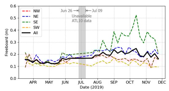
Figure 9.
Weekly variations of the average freeboards for the four sectors in the Ross Sea.
It is notable that the four sectors in the Ross Sea show their own distinctive freeboard variations. The SE sector shows the highest and most variable freeboard values compared to the other sectors. In April to May, the average of the freeboard for the SE sector is approximately 0.12–0.15 m, but it started to increase from late May. Consequently, the averaged freeboard for the SE sector reached up to 0.5 m in the second week of October, while the other sectors show freeboard less than 0.25 m. Contrary to the SE sector, the SW sector shows the lowest freeboard values for the whole year: less than 0.15 m. The freeboard in the SW sector shows relatively constant values of freeboard, without large increases or decreases. In April to June, the four sectors show only small differences in their freeboard. During June to November, however, the SE sector shows the highest increases in freeboard values, followed by NE, NW, and SW. In order to better understand the spatial and temporal variations of freeboard, we compare weekly freeboard maps and their distributions over the Ross Sea for each sector and for three seasons: the slow-freezing season (April to June), fast-freezing season (July to September), and melting season (October to November).
5.3.1. Freeboard Changes from April to June (Slow-Freezing Season)
Freeboard maps and distributions in April to June are shown in Figure 10. From April 12 to May 16, the freeboard distributions and the mean freeboard values look similar without large differences between them. Nevertheless, it is noted that the SW sector generally shows bimodal distributions such that the lower peak freeboard (~0.05 m) is lower than the other sectors (~0.1–0.15 m). This is attributed to the existence of large polynyas in the Ross Sea, especially the RISP. Clearly, the thin ice region near the RISP remains during the entire slow-freezing season from April to June (Figure 10). Two other polynyas (the TNBP and MSP) should be occasionally observed in the Ross Sea, but they are hardly overlapped with ICESat-2 tracks because of their relatively small spatial scales compared to the RISP (Figure 2). Thus, these relatively small polynyas can be only observed if the ICESat-2 tracks are exactly coincident with the occurrence of these polynya events. There was no coincidence between the ICESat-2 tracks and the TNBP or MSP polynya events during our study period. Although there is no large increase or decrease in the freeboard for all four sectors in this slow-freezing season, freeboard starts to increase in the eastern sectors (NE and SE) from the week of 24 May. In particular, the freeboard starts to increase mainly from the east side of the SE sector, which indicates the inflow of thick multiyear ice from the Amundsen Sea, east of the Ross Sea area [68,69,70].

Figure 10.
Weekly freeboard maps and freeboard distributions for the Ross Sea four sectors during April to June (slow-freezing season) 2019. Vertical dashed lines in the distributions indicate the mean of the freeboard for each sector. Black arrows on the maps indicate the location of the Amundsen Sea.
5.3.2. Freeboard Changes from July to September (Fast-Freezing Season)
Figure 11 shows the weekly freeboard maps and distribution changes during the fast-freezing season from July to September. The SW sector still shows a bimodal distribution during this season, and the first lower mode has approximately 0.05 m of freeboard, which indicates the thin ice around the RISP in this sector. The freeboard in the SE sector has dramatically increased during this period until the first week of September. The SE sector also shows a bimodal distribution, but both modal freeboards continuously shift to the right, unlike the consistent bimodal freeboard values for the SW sector. Additionally, while the right mode increases much faster, the left mode moves with similar increase rates to the NW and NE sector. It is logical that the increase in freeboard in the SE sector is mainly led by two different sources: (1) inflow of thick ice from the Amundsen Sea (greater mode), and (2) internal ice growth in the SE sector (lower mode). Thus, the SE sector shows a very wide range of freeboard compared to the other sectors. The NE and NW sectors usually show unimodal distributions, but sometimes they also show bimodal distributions. Specifically, the thin ice from the SW sector is sometimes advected into the NW sector, shown as the small mode in the distribution, and thicker ice from the SE sector is sometimes advected into the NE sector, shown as the greater mode in the distribution in these weeks.
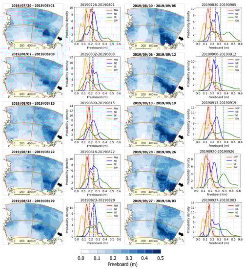
Figure 11.
Weekly freeboard maps and freeboard distributions for the Ross Sea (four sectors) during July to September (fast-freezing season) 2019. Vertical dashed lines in the distributions indicate the mean freeboard for each sector. Black arrows on the maps indicate the location of the Amundsen Sea.
5.3.3. Freeboard Changes from October to November (Melting Season)
Freeboards reached a maximum in the week of 11 October and began to decrease after that (Figure 9). During this melting season, the SW sector contains the lowest freeboard, and we can still identify the spatial distribution of the polynya-related thin ice in this sector (Figure 12). The NW sector shows the second lowest freeboard due to the impacts of thin ice advected from the SW sector. The SE sector shows the highest freeboard and the widest distribution of the freeboard, but the freeboard decreases from the week of 24 November. An interesting finding here is that the highest freeboard region shifts northward in the SE sector. During the weeks of 11–31 October, the highest freeboard regions are located in the southeast coastal area of the SE sector. As time passes, however, we can observe that these highest freeboard regions are shifted to the northern side of the SE sector (i.e., border between the SE and NE sectors) in the weeks from 1 November to 28 November. This can be associated with the movement of thick sea ice towards the north of the Ross Sea. According to previous studies [68,69,71], sea ice moves northward in this sector, so thick ice was pushed away to the north side.

Figure 12.
Weekly freeboard maps and freeboard distributions for the Ross Sea four sectors during October to November (melting season). Vertical dashed lines in the distributions indicate the mean freeboard for each sector. Black arrows on the maps indicate the location of the Amundsen Sea.
6. Discussion
6.1. Comparison with NIC Ice Chart
We compare the weekly freeboard estimated by kriging with the National Ice Center (NIC) weekly ice chart (Figure 13). The NIC ice charts are produced through the manual interpretation of various data sources including in situ, remote sensing (e.g., visible, infrared, active/passive microwave), and model outputs [72]. Although they do not provide accurate thickness measurements, they consist of multiple polygons showing the categorical stage of development of sea ice (e.g., nilas, grey ice, young ice, first-year thin ice, first-year thick ice, old ice, etc.). This ice chart data has been used to examine the spatiotemporal variations of ice thickness and volume in the Ross Sea area [69]. In this study, we convert the categorical ice type of each polygon into numerical ice thickness values using the method of DeLiberty et al. [69] Thus, since each polygon of the ice chart has a single thickness value, we compare the converted ice thickness for each polygon with the ICESat-2 freeboard averaged over that polygon.

Figure 13.
Scatter plot between weekly freeboard estimated by ICESat-2 based kriging and ice thickness from the weekly NIC ice chart for April to November 2019.
As shown in Figure 13, the kriged freeboard and the NIC ice thickness show a significant correlation (R = 0.587, p-value < 0.001) to each other. This implies that our weekly freeboard estimation agrees with the existent sea ice thickness products. Furthermore, the slope of this linear fit (2.61) is close to that from the literature that converted sea ice freeboard into ice thickness for the Ross Sea area in early spring (2.45) [73].
However, it should be noted that they do not have a perfect linear relationship because of the major differences between them. First, while our freeboard maps represent the total freeboard, the NIC ice charts represent the ice thickness. Considering the variations of snow/ice density or snow depth over the Ross Sea [74], the freeboard and ice thickness can be deviated from the complete linear fit. Second, while our freeboard maps are based on the quantitative measures from ICESat-2, the NIC ice charts are based on the manual interpretation of various data. Thus, the thickness from the NIC ice chart is not an accurate reference but a rough categorical estimation of sea ice thickness. Third, although we try to reduce the impacts of sea ice deformation using the 3 km mode sampling, our freeboard maps can still involve these dynamic impacts. In contrast, the thickness from the NIC ice chart is merely based on the thermodynamic ice growth [69]. Therefore, herein, we only check a rough coherency between our estimation and the NIC ice chart, rather than the accurate validation of our freeboard maps. We would suggest the weekly ICESat-2 freeboard maps, if they can be produced in near real-time, to be incorporated into a real-time weekly NIC ice chart to improve the potential accuracy of the chart.
6.2. Limitations of the Geostatistical Approach
This study presents a geostatistical characterization and weekly mapping of total freeboard in the Ross Sea by using ICESat-2 ATL10 products. The spatial autocorrelation ranges of ATL10 freeboard are quantified from the geostatistical variograms, and freeboards are interpolated by ordinary kriging based on these variogram models. The resulting weekly freeboard maps successfully identify the spatial distributions of polynya areas in the Ross Sea.
However, the geostatistical approach used here can have several limitations. From the statistical point of view, this method can introduce significant uncertainties if the number of ICESat-2 observations are not sufficient in a given region [75,76]. In particular, since ICESat-2 laser photons cannot penetrate into clouds, overcast weather conditions can cause a lack of measurements. This is evidenced by a somewhat discontinuous appearance in some of the freeboard maps (Figure 10, Figure 11 and Figure 12).
Another issue of the geostatistical approach used in this study is that it assumes that the sea ice across the Ross Sea remains static over a week’s period (i.e., stationarity). However, the sea ice distribution over the Ross Sea is very dynamic and can change significantly even within one week, especially in the SW sector where frequent katabatic wind events can drive significant sea ice production. Since our geostatistical kriging model is based on the assumption of static conditions for the training dataset, freeboard changes occurring with a shorter than one-week scale cannot be described by this approach.
In addition, it is also necessary to consider the assessment or validation of the ATL10 total freeboard product for the Ross Sea. Although some studies assessed the ATL10 freeboard data in comparison with other air-borne missions, such as Operation Ice Bridge (OIB) for the Arctic [59], the accuracy of ATL10 freeboard over the Ross Sea has not been evaluated. Due to the lack of validation data in the Ross Sea, the cross-validation of this study is conducted with the ATL10 freeboard product itself, rather than independent sea ice freeboard measurements. Therefore, it is necessary to assess the accuracy of the ATL10 freeboard product by using sea ice field data in the near future. In addition, herein we only analyze the freeboard values, not the sea ice thickness. Although there are several methods to convert freeboard into thickness for the Ross Sea area [28,73], it is not clear what method would best describe the sea ice conditions over Ross Sea for the entire year. Therefore, it is also critical to examine how to associate the freeboard changes with the thickness variations over the Ross Sea.
7. Summary and Conclusions
In this study, we implement a geostatistical analysis to examine the spatial autocorrelation characteristics of ICESat-2 ATL10 freeboards over the Ross Sea. Based on this spatial autocorrelation, we generate weekly freeboard maps by applying ordinary kriging to detect spatiotemporal variations of sea ice over the Ross Sea. Before applying kriging interpolation for mapping, we conduct a cross validation to check the reliability of this kriging method for freeboard mapping. According to the cross-validation results, the kriging-estimated freeboards show significant correlation (R > 0.5), RMSE ~ 0.12 m, and MAE ~ 0.7 m with the ATL10 freeboard measurements. Three different variogram models (exponential, Gaussian, and spherical) show insignificant differences in their accuracy. This cross-validation result shows that the geostatistical approach can be useful for estimating freeboards in missing spaces where ICESat-2 data are not directly available. The spatial correlation range of the variogam models indicates that the ATL10 freeboard product can statistically represent the freeboard on scales of 5–10 km from the source data track. For the area farther away from the ATL10 measurements than this effective range, the variograms show the sill values less than 0.01 m2 for April to July, but greater than that for August to November. The uncertainty of this kriging method increases in winter to spring as the ice grows, but the largest uncertainty is expected for the melting season.
The resulting weekly maps are used to examine the spatiotemporal changes of sea ice freeboard over the Ross Sea. We divided the Ross Sea into four sectors (SW, SE, NW, and NE) to better characterize short-term regional sea ice changes. Our weekly freeboard maps capture the spatial distributions of large polynya areas (i.e., RISP) over the Ross Sea. The polynya areas are mainly located in the SW sector, but sometimes they extend to the SE or NW sectors. The SW sector shows the lowest and less variable freeboard changes with bimodal freeboard distributions due to the large polynya areas in this sector. In contrast, the SE sector shows the largest and more variable changes of the freeboard from the freezing season to the melting season, which is partially attributed to the thick multiyear ice advected from the Amundsen Sea. Meanwhile, we also find that the thick ice in the SE sector drifts northward in the melting season. If our short-term freeboard mapping is combined with other multispectral or radar satellite data (e.g., Landsat, Sentinel-1, Sentinel-2), we are confident that we can efficiently estimate sea ice production in the polynya areas over the Ross Sea.
Author Contributions
Conceptualization, Y.K. and H.X.; methodology, Y.K.; writing—original draft preparation, Y.K.; writing—review and editing, H.X., N.T.K., S.F.A., A.M.M.-N. All authors have read and agreed to the published version of the manuscript.
Funding
This research was funded by U.S. NSF (1835784) and NASA (80NSSC18K0843 and 80NSSC19M0194).
Acknowledgments
We would like to thank the National Aeronautics and Space Administration (NASA) for processing and providing ICESat-2 data. Funding supports were from U.S. NSF (1835784) and NASA (80NSSC18K0843 and 80NSSC19M0194) grants. Critical reviews and constructional comments from three anonymous reviewers to improve the quality of this manuscript are greatly appreciated.
Conflicts of Interest
The authors declare no conflict of interest.
References
- Kurtz, N.T.; Markus, T. Satellite observations of Antarctic sea ice thickness and volume. J. Geophys. Res. Oceans 2012, 117, 1–9. [Google Scholar] [CrossRef]
- Allison, I.; Brandt, R.E.; Warren, S.G. East Antarctic sea ice: Albedo, thickness distribution, and snow cover. J. Geophys. Res. Oceans 1993, 98, 12417–12429. [Google Scholar] [CrossRef]
- Massom, R.A.; Eicken, H.; Hass, C.; Jeffries, M.O.; Drinkwater, M.R.; Sturm, M.; Worby, A.P.; Wu, X.; Lytle, V.I.; Ushio, S.; et al. Snow on Antarctic sea ice. Rev. Geophys. 2001, 39, 413–445. [Google Scholar] [CrossRef]
- Screen, J.A.; Simmonds, I. The central role of diminishing sea ice in recent Arctic temperature amplification. Nature 2010, 464, 1334–1337. [Google Scholar] [CrossRef]
- Brandt, R.E.; Warren, S.G.; Worby, A.P.; Grenfell, T.C. Surface Albedo of the Antarctic Sea Ice Zone. J. Clim. 2005, 18, 3606–3622. [Google Scholar] [CrossRef]
- Serreze, M.C.; Barry, R.G. Processes and impacts of Arctic amplification: A research synthesis. Glob. Planet. Chang. 2011, 77, 85–96. [Google Scholar] [CrossRef]
- Gordon, A.L. Two Stable Modes of Southern Ocean Winter Stratification. In Deep Convection and Deep Water Formation in the Oceans; Chu, P.C., Gascard, J.C., Eds.; Elsevier Oceanography Series; Elsevier: Amsterdam, The Netherlands, 1991; Volume 57, pp. 17–35. [Google Scholar]
- Cavalieri, D.J.; Parkinson, C.L. Large-Scale Variations in Observed Antarctic Sea Ice Extent and Associated Atmospheric Circulation. Mon. Weather Rev. 1981, 109, 2323–2336. [Google Scholar] [CrossRef]
- Comiso, J.C.; Gersten, R.A.; Stock, L.V.; Turner, J.; Perez, G.J.; Cho, K. Positive Trend in the Antarctic Sea Ice Cover and Associated Changes in Surface Temperature. J. Clim. 2017, 30, 2251–2267. [Google Scholar] [CrossRef] [PubMed]
- Garrison, D.L. Antarctic Sea Ice Biota. Am. Zool. 1991, 31, 17–33. [Google Scholar] [CrossRef]
- Legendre, L.; Ackley, S.F.; Dieckmann, G.S.; Gulliksen, B.; Horner, R.; Hoshiai, T.; Melnikov, I.A.; Reeburgh, W.S.; Spindler, M.; Sullivan, C.W. Ecology of sea ice biota. Polar Biol. 1992, 12, 429–444. [Google Scholar] [CrossRef]
- Kwok, R.; Rothrock, D.A. Decline in Arctic sea ice thickness from submarine and ICESat records: 1958–2008. Geophys. Res. Lett. 2009, 36. [Google Scholar] [CrossRef]
- Simmonds, I. Comparing and contrasting the behaviour of Arctic and Antarctic sea ice over the 35 year period 1979–2013. Ann. Glaciol. 2015, 56, 18–28. [Google Scholar] [CrossRef]
- Comiso, J.C.; Parkinson, C.L.; Gersten, R.; Stock, L. Accelerated decline in the Arctic sea ice cover. Geophys. Res. Lett. 2008, 35. [Google Scholar] [CrossRef]
- Kurtz, N.T.; Markus, T.; Farrell, S.L.; Worthen, D.L.; Boisvert, L.N. Observations of recent Arctic sea ice volume loss and its impact on ocean-atmosphere energy exchange and ice production. J. Geophys. Res. Oceans 2011, 116. [Google Scholar] [CrossRef]
- Notz, D.; Stroeve, J. Observed Arctic sea-ice loss directly follows anthropogenic CO2 emission. Science 2016, 354, 747–750. [Google Scholar] [CrossRef] [PubMed]
- Parkinson, C.L. A 40-y record reveals gradual Antarctic sea ice increases followed by decreases at rates far exceeding the rates seen in the Arctic. Proc. Natl. Acad. Sci. USA 2019, 116, 14414–14423. [Google Scholar] [CrossRef]
- Ludescher, J.; Yuan, N.; Bunde, A. Detecting the statistical significance of the trends in the Antarctic sea ice extent: An indication for a turning point. Clim. Dyn. 2019, 53, 237–244. [Google Scholar] [CrossRef]
- Massonnet, F.; Mathiot, P.; Fichefet, T.; Goosse, H.; König Beatty, C.; Vancoppenolle, M.; Lavergne, T. A model reconstruction of the Antarctic sea ice thickness and volume changes over 1980–2008 using data assimilation. Ocean Model. 2013, 64, 67–75. [Google Scholar] [CrossRef]
- Holland, P.R.; Bruneau, N.; Enright, C.; Losch, M.; Kurtz, N.T.; Kwok, R. Modeled trends in antarctic sea ice thickness. J. Clim. 2014, 27, 3784–3801. [Google Scholar] [CrossRef]
- Parkinson, C.L.; Cavalieri, D.J. Antarctic sea ice variability and trends, 1979–2010. Cryosphere 2012, 6, 871–880. [Google Scholar] [CrossRef]
- Yuan, N.; Ding, M.; Ludescher, J.; Bunde, A. Increase of the Antarctic Sea Ice Extent is highly significant only in the Ross Sea. Sci. Rep. 2017, 7, 41096. [Google Scholar] [CrossRef] [PubMed]
- Tamura, T.; Ohshima, K.I.; Fraser, A.D.; Williams, G.D. Sea ice production variability in Antarctic coastal polynyas. J. Geophys. Res. Oceans 2016, 121, 2967–2979. [Google Scholar] [CrossRef]
- Tamura, T.; Ohshima, K.I.; Nihashi, S. Mapping of sea ice production for Antarctic coastal polynyas. Geophys. Res. Lett. 2008, 35. [Google Scholar] [CrossRef]
- Nihashi, S.; Ohshima, K.I.; Tamura, T. Sea-Ice Production in Antarctic Coastal Polynyas Estimated from AMSR2 Data and Its Validation Using AMSR-E and SSM/I-SSMIS Data. IEEE J. Sel. Top. Appl. Earth Obs. Remote Sens. 2017, 10, 3912. [Google Scholar] [CrossRef]
- Tian, L.; Xie, H.; Ackley, S.F.; Tang, J.; Mestas-Nuñez, A.M.; Wang, X. Sea-ice freeboard and thickness in the Ross Sea from airborne (IceBridge 2013) and satellite (ICESat 2003–2008) observations. Ann. Glaciol. 2020, 61, 24–39. [Google Scholar] [CrossRef]
- Dai, L.; Xie, H.; Ackley, S.F.; Mestas-Nuñez, A.M. Ice Production in Ross Ice Shelf Polynyas during 2017–2018 from Sentinel–1 SAR Images. Remote Sens. 2020, 12, 1484. [Google Scholar] [CrossRef]
- Li, H.; Xie, H.; Kern, S.; Wan, W.; Ozsoy, B.; Ackley, S.; Hong, Y. Spatio-temporal variability of Antarctic sea-ice thickness and volume obtained from ICESat data using an innovative algorithm. Remote Sens. Environ. 2018, 219, 44–61. [Google Scholar] [CrossRef]
- Drucker, R.; Martin, S.; Kwok, R. Sea ice production and export from coastal polynyas in the Weddell and Ross Seas. Geophys. Res. Lett. 2011, 38. [Google Scholar] [CrossRef]
- Tin, T.; Jeffries, M.O. Sea-ice thickness and roughness in the Ross Sea, Antartica. Ann. Glaciol. 2001, 33, 187–193. [Google Scholar] [CrossRef]
- Markus, T.; Neumann, T.; Martino, A.; Abdalati, W.; Brunt, K.; Csatho, B.; Farrell, S.; Fricker, H.; Gardner, A.; Harding, D.; et al. The Ice, Cloud, and land Elevation Satellite-2 (ICESat-2): Science requirements, concept, and implementation. Remote Sens. Environ. 2017, 190, 260–273. [Google Scholar] [CrossRef]
- Magruder, L.A.; Brunt, K.M.; Alonzo, M. Early icesat-2 on-orbit geolocation validation using ground-based corner cube retro-reflectors. Remote Sens. 2020, 12, 3653. [Google Scholar] [CrossRef]
- Zwally, H.J.; Schutz, B.; Abdalati, W.; Abshire, J.; Bentley, C.; Brenner, A.; Bufton, J.; Dezio, J.; Hancock, D.; Harding, D.; et al. ICESat’s laser measurements of polar ice, atmosphere, ocean, and land. J. Geodyn. 2002, 34, 405–445. [Google Scholar] [CrossRef]
- Kacimi, S.; Kwok, R. The Antarctic sea ice cover from ICESat-2 and CryoSat-2: Freeboard, snow depth and ice thickness. Cryosph. Discuss. 2020, 14, 4453–4474. [Google Scholar] [CrossRef]
- Petty, A.A.; Kurtz, N.T.; Kwok, R.; Markus, T.; Neumann, T. Winter Arctic sea ice thickness from ICESat-2 freeboards. J. Geophys. Res. Oceans 2020, 125, e2019JC015764. [Google Scholar] [CrossRef]
- Kwok, R.; Kacimi, S.; Webster, M.A.; Kurtz, N.T.; Petty, A.A. Arctic Snow Depth and Sea Ice Thickness From ICESat-2 and CryoSat-2 Freeboards: A First Examination. J. Geophys. Res. Oceans 2020, 125, 1–19. [Google Scholar] [CrossRef]
- Kwok, R.; Markus, T.; Kurtz, N.T.; Petty, A.A.; Neumann, T.A.; Farrell, S.L.; Cunningham, G.F.; Hancock, D.W.; Ivanoff, A.; Wimert, J.T. Surface Height and Sea Ice Freeboard of the Arctic Ocean From ICESat-2: Characteristics and Early Results. J. Geophys. Res. Oceans 2019, 124, 6942–6959. [Google Scholar] [CrossRef]
- Bromwich, D.; Liu, Z.; Rogers, A.N.; Van Woert, M.L. Winter Atmospheric Forcing of the Ross Sea Polynya. Ocean Ice Atmos. Interact. Antarct. Continenal Margin 1998, 75, 101–133. [Google Scholar]
- Dale, E.R.; McDonald, A.J.; Coggins, J.H.J.; Rack, W. Atmospheric forcing of sea ice anomalies in the Ross Sea polynya region. Cryosphere 2017, 11, 267–280. [Google Scholar] [CrossRef]
- Kwok, R.; Comiso, J.C.; Martin, S.; Drucker, R. Ross Sea polynyas: Response of ice concentration retrievals to large areas of thin ice. J. Geophys. Res. Oceans 2007, 112. [Google Scholar] [CrossRef]
- Li, J.; Heap, A.D. A review of comparative studies of spatial interpolation methods in environmental sciences: Performance and impact factors. Ecol. Inform. 2011, 6, 228–241. [Google Scholar] [CrossRef]
- Chang, K.-T. Introduction to Geographic Information Systems, 8th ed.; McGraw-Hill Education: New York, NY, USA, 2016; ISBN 9780078095139. [Google Scholar]
- Krige, D.G. A statistical approach to some basic mine valuation problems on the Witwatersrand. J. Soc. Afr. Inst. Min. Metall. 1951, 52, 119–139. [Google Scholar]
- Herzfeld, U.C.; Maslanik, J.A.; Sturm, M. Geostatistical characterization of snow-depth structures on sea ice near Point Barrow, Alaska—A contribution to the AMSR-Ice03 field validation campaign. IEEE Trans. Geosci. Remote Sens. 2006, 44, 3038–3056. [Google Scholar] [CrossRef]
- Iacozza, J.; Barber, D.G. An examination of the distribution of snow on sea-ice. Atmos. Ocean 1999, 37, 21–51. [Google Scholar] [CrossRef]
- Huang, C.L.; Wang, H.W.; Hou, J.L. Estimating spatial distribution of daily snow depth with kriging methods: Combination of MODIS snow cover area data and ground-based observations. Cryosph. Discuss. 2015, 9, 4997–5020. [Google Scholar]
- Stosius, R.; Herzfeld, U.C. Geostatistical estimation from radar altimeter data with respect to morphological units outlined by SAR data: Application to Lambert Glacier/Amery Ice shelf, East Antarctica. Ann. Glaciol. 2004, 39, 251–255. [Google Scholar] [CrossRef]
- Griggs, J.A.; Bamber, J.L. Antarctic ice-shelf thickness from satellite radar altimetry. J. Glaciol. 2011, 57, 485–498. [Google Scholar] [CrossRef]
- Strößenreuther, U.; Horwath, M.; Schröder, L. How Different Analysis and Interpolation Methods Affect the Accuracy of Ice Surface Elevation Changes Inferred from Satellite Altimetry. Math. Geosci. 2020, 52, 499–525. [Google Scholar] [CrossRef]
- Hurkmans, R.T.W.L.; Bamber, J.L.; Srensen, L.S.; Joughin, I.R.; Davis, C.H.; Krabill, W.B. Spatiotemporal interpolation of elevation changes derived from satellite altimetry for Jakobshavn Isbr, Greenland. J. Geophys. Res. Earth Surf. 2012, 117, 1–16. [Google Scholar] [CrossRef]
- Hurkmans, R.T.W.L.; Bamber, J.L.; Davis, C.H.; Joughin, I.R.; Khvorostovsky, K.S.; Smith, B.S.; Schoen, N. Time-evolving mass loss of the Greenland Ice Sheet from satellite altimetry. Cryosphere 2014, 8, 1725–1740. [Google Scholar] [CrossRef]
- Lindsay, R.; Haas, C.; Hendricks, S.; Hunkeler, P.; Kurtz, N.; Paden, J.; Panzer, B.; Sonntag, J.; Yungel, J.; Zhang, J. Seasonal forecasts of Arctic sea ice initialized with observations of ice thickness. Geophys. Res. Lett. 2012, 39, 1–6. [Google Scholar] [CrossRef]
- Kurtz, N.T.; Farrell, S.L.; Studinger, M.; Galin, N.; Harbeck, J.P.; Lindsay, R.; Onana, V.D.; Panzer, B.; Sonntag, J.G. Sea ice thickness, freeboard, and snow depth products from Operation IceBridge airborne data. Cryosphere 2013, 7, 1035–1056. [Google Scholar] [CrossRef]
- Wang, Y.; Hou, S. A new interpolation method for Antarctic surface temperature. Prog. Nat. Sci. 2009, 19, 1843–1849. [Google Scholar] [CrossRef]
- Herzfeld, U.C.; Mayer, H.; Feller, W.; Mimler, M. Geostatistical analysis of glacier-roughness data. Ann. Glaciol. 2000, 30, 235–242. [Google Scholar] [CrossRef]
- Smith, S.D.; Muench, R.D.; Pease, C.H. Polynyas and leads: An overview of physical processes and environment. J. Geophys. Res. Oceans 1990, 95, 9461–9479. [Google Scholar] [CrossRef]
- Bromwich, D.H.; Carrasco, J.F.; Liu, Z.; Tzeng, R.-Y. Hemispheric atmospheric variations and oceanographic impacts associated with katabatic surges across the Ross ice shelf, Antarctica. J. Geophys. Res. Atmos. 1993, 98, 13045–13062. [Google Scholar] [CrossRef]
- Thompson, L.; Smith, M.; Thomson, J.; Stammerjohn, S.; Ackley, S.; Loose, B. Frazil ice growth and production during katabatic wind events in the Ross Sea, Antarctica. Cryosphere 2020, 14, 3329–3347. [Google Scholar] [CrossRef]
- Kwok, R.; Kacimi, S.; Markus, T.; Kurtz, N.T.; Studinger, M.; Sonntag, J.G.; Manizade, S.S.; Boisvert, L.N.; Harbeck, J.P. ICESat-2 Surface Height and Sea Ice Freeboard Assessed With ATM Lidar Acquisitions From Operation IceBridge. Geophys. Res. Lett. 2019, 46, 11228–11236. [Google Scholar] [CrossRef]
- Kwok, R.; Cunningham, G.; Hancock, D.; Ivanoff, A.; Wimert, J. Algorithm Theoretical Basis Document (ATBD): Sea Ice Products; NASA Goddard Space Flight Center: Greenbelt, MD, USA, 2019. [Google Scholar]
- Abzalov, M. Introduction to Geostatistics. In Applied Mining Geology; Springer International Publishing: Cham, Switzerland, 2016; pp. 233–237. ISBN 978-3-319-39264-6. [Google Scholar]
- Landy, J.C.; Petty, A.A.; Tsamados, M.; Stroeve, J.C. Sea ice roughness overlooked as a key source of uncertainty in CryoSat-2 ice freeboard retrievals. J. Geophys. Res. Oceans 2020, 125, e2019JC015820. [Google Scholar] [CrossRef]
- Farrell, S.L.; Kurtz, N.; Connor, L.N.; Elder, B.C.; Leuschen, C.; Markus, T.; McAdoo, D.C.; Panzer, B.; Richter-Menge, J.; Sonntag, J.G. A first assessment of IceBridge Snow and Ice thickness data over arctic sea ice. IEEE Trans. Geosci. Remote Sens. 2012, 50, 2098–2111. [Google Scholar] [CrossRef]
- Hansen, E.; Gerland, S.; Granskog, M.A.; Pavlova, O.; Renner, A.H.H.; Haapala, J.; Løyning, T.B.; Tschudi, M. Thinning of Arctic sea ice observed in Fram Strait: 1990–2011. J. Geophys. Res. Oceans 2013, 118, 5202–5221. [Google Scholar] [CrossRef]
- Kwok, R.; Cunningham, G.F.; Kacimi, S.; Webster, M.A.; Kurtz, N.T.; Petty, A.A. Decay of the Snow Cover Over Arctic Sea Ice From ICESat-2 Acquisitions During Summer Melt in 2019. Geophys. Res. Lett. 2020, 47, 1–10. [Google Scholar] [CrossRef]
- Schober, P.; Schwarte, L.A. Correlation coefficients: Appropriate use and interpretation. Anesth. Analg. 2018, 126, 1763–1768. [Google Scholar] [CrossRef] [PubMed]
- Rack, W.; Price, D.; Haas, C.; Langhorne, P.J.; Leonard, G.H. Sea Ice Thickness in the Western Ross Sea. Geophys. Res. Lett. 2020, 48, e2020GL090866. [Google Scholar]
- Kwok, R.; Pang, S.S.; Kacimi, S. Sea ice drift in the Southern Ocean: Regional patterns, variability, and trends. Elem. Sci. Anthr. 2017, 5, 32. [Google Scholar] [CrossRef]
- DeLiberty, T.L.; Geiger, C.A.; Ackley, S.F.; Worby, A.P.; Van Woert, M.L. Estimating the annual cycle of sea-ice thickness and volume in the Ross Sea. Deep Sea Res. Part II Top. Stud. Oceanogr. 2011, 58, 1250–1260. [Google Scholar] [CrossRef]
- Worby, A.P.; Geiger, C.A.; Paget, M.J.; Van Woert, M.L.; Ackley, S.F.; DeLiberty, T.L. Thickness distribution of Antarctic sea ice. J. Geophys. Res. Oceans 2008, 113, 1–14. [Google Scholar] [CrossRef]
- Kwok, R. Ross sea ice motion, area flux, and deformation. J. Clim. 2005, 18, 3759–3776. [Google Scholar] [CrossRef]
- U.S. National Ice Center. National Ice Center Arctic Sea Ice Charts and Climatologies in Gridded Format; U.S. National Ice Center: Suitland, MD, USA, 2006; p. 41. [Google Scholar]
- Ozsoy-Cicek, B.; Ackley, S.; Xie, H.; Yi, D.; Zwally, J. Sea ice thickness retrieval algorithms based on in situ surface elevation and thickness values for application to altimetry. J. Geophys. Res. Oceans 2013, 118, 3807–3822. [Google Scholar] [CrossRef]
- Ackley, S.F.; Stammerjohn, S.; Maksym, T.; Smith, M.; Cassano, J.; Guest, P.; Tison, J.L.; Delille, B.; Loose, B.; Sedwick, P.; et al. Sea-ice production and air/ice/ocean/biogeochemistry interactions in the Ross Sea during the PIPERS 2017 autumn field campaign. Ann. Glaciol. 2020, 61, 181–195. [Google Scholar] [CrossRef]
- Webster, R.; Oliver, M.A. How Large a Sample Is Needed to Estimate the Regional Variogram Adequately? BT—Geostatistics Tróia ’92: Volume 1; Soares, A., Ed.; Springer: Dordrecht, The Netherlands, 1993; pp. 155–166. ISBN 978-94-011-1739-5. [Google Scholar]
- Webster, R.; Oliver, M.A. Sample adequately to estimate variograms of soil properties. J. Soil Sci. 1992, 43, 177–192. [Google Scholar] [CrossRef]


Publisher’s Note: MDPI stays neutral with regard to jurisdictional claims in published maps and institutional affiliations. |
© 2021 by the authors. Licensee MDPI, Basel, Switzerland. This article is an open access article distributed under the terms and conditions of the Creative Commons Attribution (CC BY) license (https://creativecommons.org/licenses/by/4.0/).