Article

Horizontal Visibility in Forests

1
Tartu Observatory, University of Tartu, 61602 Tõravere, Estonia
2
Institute of Forestry and Rural Engineering, Estonian University of Life Sciences, Kreutzwaldi 5, 51014 Tartu, Estonia
3
Military Academy, Riia 12, 51010 Tartu, Estonia
4
Forest Department, Estonian Environment Agency, Mustamäe Tee 33, 10616 Tallinn, Estonia
*
Author to whom correspondence should be addressed.
Remote Sens. 2021, 13(21), 4455; https://doi.org/10.3390/rs13214455
Submission received: 2 September 2021 / Revised: 18 October 2021 / Accepted: 1 November 2021 / Published: 5 November 2021
(This article belongs to the Section Forest Remote Sensing)

Abstract

:
The important variable of horizontal visibility within forest stands is gaining increasing attention in studies and applications involving terrestrial laser scanning (TLS), photographic measurements of forest structure, and autonomous mobility. We investigated distributions of visibility distance, open arc length, and shaded arc length in three mature forest stands. Our analysis was based (1) on tree position maps and TLS data collected in 2013 and 2019 with three different scanners, and (2) on simulated digital twins of the forest stands, constructed with two pattern-generation models incorporating commonly used indices of tree position clumping. The model simulations were found to yield values for visibility almost identical to those calculated from the corresponding tree location maps. The TLS measurements, however, were found to diverge notably from the simulations. Overall, the probability of free line of sight was found to decrease exponentially with distance to target, and the probabilities of open arc length and shaded arc length were found to decrease and increase, respectively, with distance from the observer. The TLS measurements, which are sensitive to forest understory vegetation, were found to indicate increased visibility after vegetation removal. Our chosen visibility prediction models support practical forest management, being based on common forest inventory parameters and on widely used forest structure indices.

Graphical Abstract

1. Introduction

Various kinds of forest ecosystems have one common property: the visibility distance is shorter within forested than within open terrain, because stems, branches, leaves, and needles are opaque. The shading effect of forest canopy enhances the privacy of exurban houses at landscape level [1]. Further, trees at closer range block direct rays of sight. Three-dimensional models of forests are nowadays in widespread use as tools for landscape management planning [2,3,4], and a particular interest in single-tree data arises from the need for forest management planning, tree growth and ecosystem modeling [5,6,7], and the deployment of participatory forest management systems [8]. Aerial photography has been a major data collection method over forested landscapes, indispensable in the furnishing of forest inventories [9,10] with stereophotos. Given a suitable choice of scale, individual trees can be identified and mapped from aerial photos. Additionally, however, various active systems (laser scanners), registering the reflection point coordinates of a laser pulse [11], have for more than a decade been mounted on aircraft, with an accompanying development of models for the prediction of principal forest inventory variables [12,13,14]. Airborne laser scanner data are used for predictions both of forest height [15] and of a key determinant of vertical visibility in a given forest, its canopy cover [16].
Laser scanners have been constructed also for terrestrial measurements, enabling the assessment of horizontal visibility. Such devices can provide point clouds for their environs, with a distance between pulse-reflection positions less than 10 mm at 10 m radius as measured from the scanners [17], and with the radius of the sounding beam at a 10 m distance from scanner lying in the range 1–5 mm [18]. To support tree detection from the point clouds, various algorithms have been developed for estimating tree height h and stem diameter d h at a given particular height. An international benchmarking experiment has recently been conducted [17] to compare the algorithms and scanners on a common set of forest stands. The authors of Liang et al. [17] point out that it is visibility in forest that is the chief factor in determining the precision and accuracy of forest inventory variables. The authors of Liang et al. [17] assert, on the basis of intuition, that occlusion effects of single trees become more pronounced with increasing stand density N and with decreasing mean stem diameter at breast height D 1.3 . The probability of detecting trees in a given forest from terrestrial laser scanning (TLS) data becomes smaller when the distance between scanner and tree increases [19,20]. The visibility distance v is related to occlusion of individual trees, being a function of tree location pattern, of D 1.3 , N, and the position of tree crowns relative to the line of sight in the forest.
Horizontal visibility has been an important parameter in the tactical planning of military operations, with short observation zones characteristic of wooded, as opposed to open, terrain, and with visibility between trees taken as a basic factor in selecting movement, orientation, and fields of fire [21]. Additionally, the operations of unmanned ground vehicles and autonomous robots executing particular forest management tasks [22] can be optimized when maps of visibility estimates at sufficiently fine spatial resolution are constructed for the target area. In forest inventory fieldwork, preliminary estimates of v and its distribution function help in the selecting of location schemes and in the determining of an optimum number of observation points for TLS devices [23].
Different definitions of visibility exist. In the case of a human observer, it is important to include the properties of the target object (its color, shape, and size), the minimum time of the visual contact, the requirements for determining type of the target object, and the (relative) movement of the target and the observer [24,25]. For a human eye with excellent acuity, the finest theoretical resolution is 50–60″ [26]. In the complex visible scene in a forest, however, this limiting resolution cannot be attained. Instrumental measurements of visibility distance can be made via digital photographic cameras or TLS devices [27,28], with the obtained quantity representing horizontal gap fraction per unit of selected distance. The prediction of mean path length v ¯ , for a probability corresponding to zero contacts of the probe with tree stems, is possible under the assumption of a Poisson distribution for tree stem positions, provided D 1.3 and N are known from a forest inventory database [29]. Deviations from the random tree-location pattern can be computed by means similar to the solution used in the radiative transfer model FRT [30], i.e., by correcting the stand density by the factor σ N 2 / N , where σ N 2 is the variance of N.
Although mean values of visibility distance are reported in the literature [24,25,31], the distribution of v is rarely studied. For this paper, we analyzed TLS measurements from three mature hemiboreal forest stands of different structure, to obtain distributions of v and of open arc length φ o . TLS measurements were taken with three different scanners in 2013 and 2019. The angular resolution of the TLS measurements in the forests was in agreement with practical human visibility, as limited by the resolution of a human eye. An experiment of forest understory removal was carried out in one stand. The influence of tree location pattern on the distribution of v was studied with two models.
We sought to construct visibility prediction models that employ common forest inventory parameters and forest structure indices, and that could therefore be used in practical forest management planning in combination with TLS scanning data. (1) We used an electrostatic model of the work in Gusakov and Fradkin [32], simulating positions of trees and accounting for deviations from the Poisson distribution. (2) We used a stand pattern progress model (STPP), first taking an initial dense random tree pattern, and then applying an assumed yearly mortality rate to remove trees according to a process parameter. With both models, the driving parameter values for our tree location pattern simulations were selected on the basis of stand structure indices (see, e.g., in [32,33,34,35,36,37]) calculated from tree mapping data.

2. Materials and Methods

Measurements of forest structure with TLS were carried out in three mature hemiboreal forest stands in southeastern Estonia at the Järvselja remote sensing test site. Detailed measurements of stand structure were carried out in the summer of 2007, as reported in Kuusk et al. [38]. The sample plots were those which had been previously established for the Radiative Transfer Model Intercomparison (RAMI) experiment [39].
Järvselja forests are typical for the hemiboreal zone, the dominant tree species being Scots pine (Pinus sylvestris L.), Norway spruce (Picea abies Karst.), silver and white birch (Betula pendula Roth, Betula pubescens Ehrh.), European aspen (Populus tremula L.), and common and white alder (Alnus glutinosa (L.) Gaertn., Alnus incana (L.) Moench). All these species can grow in pure or mixed stands. Growth conditions in Järvelja range from poor where H 100 (stand height at the stand age of 100 years) is less than 10 m to very good where H 100 can be over 35 m.
The Järvselja RAMI birch stand is a typical mixed broadleaf stand in the hemiboreal zone, growing on brown gleysol. Growth conditions were good, with the site index H 100 at 28.7 m. The stand age was 49 years in 2007. The dominating species according to basal area were silver birch (57%), common alder (30%), and European aspen (11%). The stocking density was 940 trees per hectare. Two tree layers were distinguishable according to the social status of the trees. The lower tree layer mostly consisted of lime (Tilia cordata Mill.) and Norway spruce. The coordinates of the stand center are 58°17 N, 27°20 E.
The Järvselja RAMI pine stand grows on transitional bog. The soil is deep (>1.3 m) Sphagnum peat. Growth conditions were poor, as indicated the H 100 value of 10.8 in the forest inventory database. In 2007, the stand height was 15.6 m, stand age was 125 years, and stand density of the dominant layer was 1115 trees per hectare. Forest understory vegetation was composed of Ledum palustre Harmaja, sparse Eriophorum vaginatum L., and a continuous Sphagnum spp. moss layer. The coordinates of the stand center are 58°19 N, 27°18 E.
The Järvselja RAMI spruce stand grows on a gleyi-ferric podzol site. Growth conditions were rather good (with H 100 = 29.1), as a consequence of favorable drainage. The stand age was 59 years in 2007. Two tree layers were distinguishable according to the social status of the trees. Average height in the first (upper) layer was 23.2 m, with a density of 774 trees per hectare. Stand density in the second (lower) layer was 915 trees per hectare, with the tree height range 3.5–20 m. As the canopy cover was high (0.89), forest understory vegetation either was partially missing or consisted only of mosses, such as Hylocomium splendens (Hedw.) Schimp. or Pleurozium schreberi (Brid.) Mitt. The coordinates of the stand center are 58°18 N, 27°15 E.
A summary of stand parameters, from the 2007 inventory, is given in Table 1. Changes in the structure of the stands between 2007 and 2019 are reported by Lang et al. [40].

2.1. Field Measurements and Data Processing

In July 2013, the stands were measured with the TLS Leica ScanStation C10, and in August 2019 both with the TLS Leica RT360 and with the Trimble SX10 Scanning Total Station. The Trimble SX10 was used in a combined land-survey mode, in which the TLS speed and range are limited. All three TLS measurements were carried out on a regular grid of 9 permanent sampling points (L1–L9) with a spatial step of 30 m ( x , y = 20 m, 50 m, 80 m), see [38] for details of the grid. Further, in 2013 the pine and birch stands were measured with high point density in 6 points around the central sampling point (L5). In August 2019, 125 points, separated from each other by about 10 m, were additionally measured in the pine stand. The parameters of the laser scanners used are given in Table 2, and parameters of TLS measurements in the RAMI stands in Table 3.
In every measurement point, a slice of thickness 20 cm at the level of the scanner head was extracted from the point cloud, and distance and azimuth were found for each laser hit in the slice. The azimuthal ring of 360° was divided into 7200 (resp. 3600) azimuthal sectors for high (resp. low) density measurements, with a consequent angular step of <0.05° (resp. of 0.05–0.1°). In every azimuthal sector, the hits were separated into 13 distance cells, with distances ranges 1–2 m, 2–3 m, 3–4 m, 4–5 m, 5–7 m, 7–10 m, 10–15 m, 15–20 m, 20–30 m, 30–40 m, 40–50 m, 50–70 m, and 70–100 m. Initially, all cells were set to the value 1 (indicating a gap). Where a laser hit fell into a cell, the value of that cell and of all more distant cells in the sector was reset to 0, as shown in Figure 1. Under this representation, the probability of a free line of sight (FLoS) of length l j becomes
p ( l j ) = 1 n i g i , j
where g i , j is the cell value in the ith azimuth sector at the distance l j and n is the number of azimuthal sectors (3600 or 7200).

2.2. Simulation of Tree Pattern

For the theoretical analysis of horizontal visibility in forests, we used two different procedures for generating tree patterns in a stand, taking on the one hand the electrostatic model in Gusakov and Fradkin [32] and on the other the stand pattern progress model STPP. Geometrical parameters of stands (stand density, the diameter at breast height (DBH) of tree stems, and the pattern regularity) were set in correspondence with mean values in the RAMI stands. Visibility in the generated-pattern stand was analyzed in a way similar to the processing of TLS point clouds: the position of every tree stem in the ( d , φ ) space was found, and the angular sector containing each found tree stem was marked as being in shade, starting from the cell containing the tree stem (Figure 1).

2.2.1. Electrostatic Model

In the electrostatic model of Gusakov and Fradkin [32], a random pattern of tree positions is first generated, and then trees are moved relative to each other, under the influence of a hypothesized attractive or repulsive force between trees, until the given structure is reached, with its particular degree of clumping or regularity. The input parameters of the model are the stand density, the distance of incidence where trees interact, and the power and nature (specified as either attractive or repulsive) of their interaction.

2.2.2. Pattern Progress Model

The stand pattern progress model STTP simulates the development of a stand pattern over time. Initially a dense ( N 0 ) random pattern of plants is generated and a random weight w ( 0 < w 1 ) is assigned to every plant.
In every year some given fraction q of trees of the lowest weight falls out, due to self-thinning from competition-induced mortality. The stand density consequently decreases every year. The final pattern of tree positions is governed by the stand age A, under the rule N = N 0 ( 1 q ) A specifying how trees fall out. As an alternative to a constant parameter q for self-thinning, the thinning parameter can be linked to some growth function such as DBH or tree height H, dependent on stand age A [41]. Varying the rules of self-thinning makes it possible to simulate tree patterns of a given regularity. If the trees which fall out are selected randomly (i.e., independently of the given weight and independently of distance from neighbors), then the final pattern will likewise be random.
Another option is to have only some fraction γ q of trees removed randomly, with the others subject to removal under some given selection rules: if two trees are very close to each other and their weights do not differ greatly, both will survive, developing a common crown, and where these conditions are not met, the tree of smaller weight will be removed, with its neighbor remaining. The process is repeated until the required number of trees has been removed.
As another modeling option, it can be stipulated that if the weights of two neighboring trees do not differ greatly, then the tree on the sunlit side survives and the tree in shade dies. Repeating this procedure for a given run of years yields the final density of the stimulated stand, presenting the given regularity. If nearest neighbors are removed, the procedure generates regular patterns. The highest regularity is reached when the only rule for removing a tree is that the distance to nearest neighbor is to be minimal within the stand. The level of maximal possible regularity is controlled by the fraction q, specifying what percentage of trees fall out every year. If the removed tree is the one with maximal distance to its nearest neighbor, then the final stand will have a clumped pattern. It is, however, difficult to give reasons why in an even-aged stand a tree with no close neighbors should fall out.

2.2.3. Indices for the Description of Tree Distribution

Several indices have been suggested for the description of the tree pattern in a forest stand [32,33,34,35,36,37]. Structure indices can be divided into three groups: (A) as those based on the number of trees in a test area, (B) as those based on distances between trees, and (C) as those based on the angular structure of the positions of a few nearest trees. In this investigation, we used seven different indices, each of which we had in this investigation found to depend monotonically on the stand-generation parameters applied in models.
(A) In area methods, the variation of tree number over a sample area is analyzed. If the distribution pattern is random, the frequencies follow a Poisson distribution. In this Poisson case, it is expected that the relative variance F = σ n 2 / N m , where N m is the mean number of trees, is unity, i.e., that F = 1 . In the case of a regular pattern, F < 1 , and for a clumped pattern F > 1 . The index F is called Fisher’s grouping index [42] or grouping index Cox I [33]. Nilson [42] introduced the grouping index c, as a nonlinear function of Fisher’s grouping index F, setting c ( θ ) = ( ln ( 1 ( 1 a ( θ ) ) ( 1 F ) ) ) / ( 1 F ) , where a ( θ ) is the transparency of a tree crown at zenith angle θ . In Nilson [42], the index c is expressed for a positive binomial distribution of trees. These various indices depend on probe area. A common selection for the probe area is the area of tree-crown vertical projection S = π R c r 2 , where R c r is the crown radius. An alternative selection is the mean area per tree in a stand, S = 1 / N .
(B) In distance methods, the simplest index is the mean distance to the nearest neighbor in the case of a random pattern, with l r a n d o m = 1 / ( 2 N ) .
The distance l r a n d o m does not describe the regularity of the tree pattern, being simply a direct function of stand density. A quantity which does depend on the tree pattern in a stand, however, is the mean distance to nearest neighbor, l n n [43]. In stands of some fixed density N, l n n increases with increasing regularity of the stand. Since l n n depends on stand density, a better choice is the relative distance l n n / l r a n d o m . In a random stand l n n / l r a n d o m = 1 . With increasing regularity this ratio increases, and in a clumped stand l n n / l r a n d o m < 1 .
The Hopkins index is the ratio of the squared distance from a random point to the nearest tree, l r , 1 2 , to the squared distance to the nearest neighbor, l n n 2 , namely, I H = l r , 1 2 / l n n 2 [33,36] (with the angle brackets here marking averaging). In random, regular, and clumped stands respectively, I H = 1 , I H < 1 , and I H > 1 .
A modified version of Clark–Evans index compares the smallest distance from a random point to a second nearest tree, l r , 2 , with the mean distance l m e a n = 1 / ( 2 N ) , as I C E F = l r , 2 / l m e a n [32]. In a regular stand I C E F > 1 , and in a clumped stand I C E F < 1 .
The work in Diggle [44] suggests a two-stage procedure for distinguishing spatial point patterns as regular, random-homogeneous, random-heterogeneous, or aggregated. For m randomly selected points the statistics of u i = l r , 1 2 + l r , 2 2 / 2 are analyzed, where l r , 1 and l r , 2 are the respective distances to the nearest tree and to the next nearest tree.
(C) In an angular-structure method, the stand pattern is characterized by statistics of azimuths for some small number of nearest trees. The authors of Gadow et al. [45] propose as a structure parameter the ‘Winkelmass’ neighborhood pattern, noting that in a uniform pattern the mean angle between the n nearest neighbors is 360 ° / n , and suggesting that in practical applications four neighbors be taken. Formally, this becomes
W i = 1 4 j = 1 4 ν j
where ν j is a binary variable, defined as ν j = 1 if α j < α 0 and as ν j = 0 otherwise, and where α 0 is some specified standard angle. Gadow and Hui [34] suggest the standard value α 0 = 72 ° for the Winkelmass of four neighbors. Random, regular, and clumped patterns then yield, respectively, W = 0.496 , W < 0.496 , and W > 0.496 .

2.3. Using Structure Indices in the Tree Location Pattern Simulation Model STPP

To overcome implementation difficulties resulting from differences among the various principles underlying our selected set of structure indices, we constructed a lookup table, to let us select corresponding values of the parameter γ for each index. The construction was found by first conducting a series of pattern simulations with the STPP model, varying γ from 0 to 1, and then calculating structure index values for the γ -driven run of patterns.
For each RAMI stand, it was now possible to look up a γ value for each structure index in our set, according to the index values calculated for the field inventory data (Table 4). Finally, for visibility analyses, the largest and smallest γ values for each RAMI stand were found from the lookup table, according to the structure index values given in Table 4, and the corresponding patterns were simulated.

3. Results

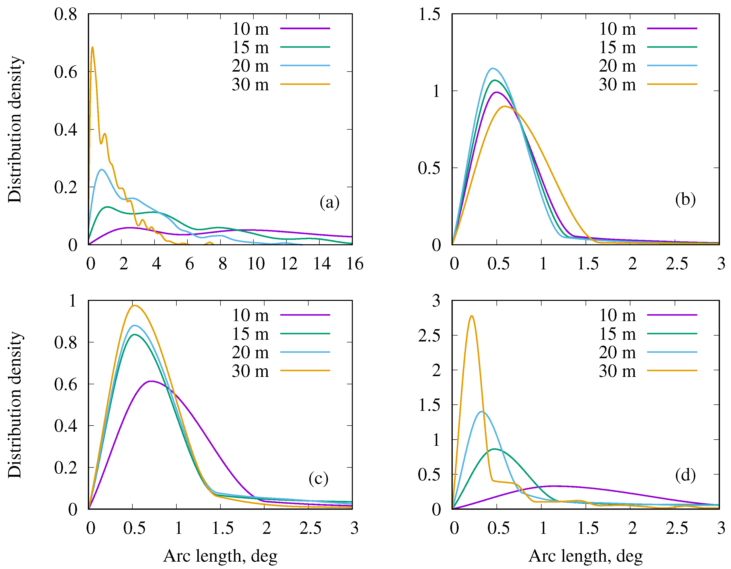
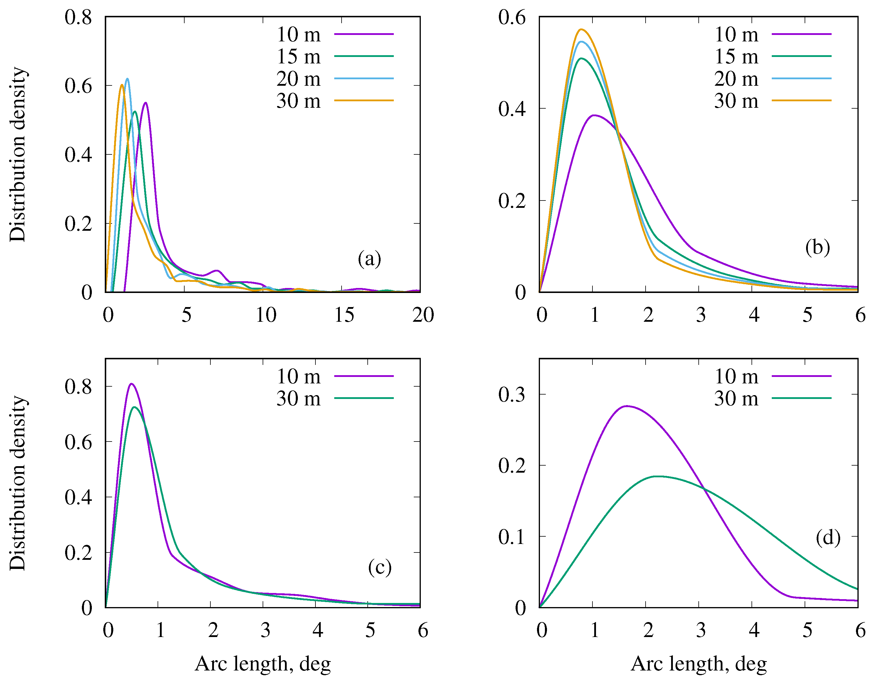
3.1. Horizontal Visibility

Figure 2, Figure 3 and Figure 4 present the probability of FLoS in the three RAMI stands: (i) as computed from the models, (ii) as computed from RAMI-database measurements of tree positions and stem diameters, and (iii) as estimated from the TLS point clouds generated by the three different scanners (with four different field sessions, Leica 2013 , Trimble 2019 , Leica 2019 , and Leica 2019 tr in the case of the pine stand, and with three different field sessions, Leica 2013 , Trimble 2019 , and Leica 2019 , in the case both of birch stand and of spruce stand). Tree positions were given in the RAMI database for plots measuring 100 m × 100 m. Consequently, in the eight permanent sampling points, no tree positions were available from sectors in some directions at distances exceeding 20 m. The visibility values at 30 m and 40 m in Figure 2, Figure 3 and Figure 4, in the curves marked ‘RAMI’, are therefore overestimated. In the simulations with tree pattern models, the plot size was set to 200 m × 200 m, with each measurement position near the center of its plot, as in the TLS measurement. The error bars in Figure 2 signify standard deviation in FLoS. The variability of estimated probability, as Equation (1), in the birch and spruce stands was found to be comparable to the variation in the pine stand shown in Figure 2.
In all three stands, visibility values from the model calculations were found to be higher than the values estimated from the TLS point cloud. While all four TLS measurements coincided in the pine stand, yielding an estimated FLoS probability of 50% at 25 m, the same probability was attained in the model simulations at 35 m. The following are possible reasons for the discrepancy: (1) Whereas in the model simulations the line of sight is a ray of zero diameter, the TLS sounding beam has a nonzero diameter, on the order of 5–7 mm; (2) vibration of the TLS instrument during measurements in field conditions may smear out the hit position to some extent, increasing the visible diameter of tree stems; and (3) the applied TLS-method estimates the maximum diameter of stems controlled by the roughness of stem bark, in place of estimating the mean diameter at breast height.
Figure 3 shows discrepancies to be large in the birch stand. Although two independent TLS measurements in 2019 agreed well at distances exceeding 10 m, there were some discrepancies at short distances in 2019, and also substantial differences in FLoS in different years. It is possible that there were small differences in the position and height of the scanner’s optical head between the Trimble 2019 and the Leica 2019 measurements. Furthermore, the Leica 2019 measurements were taken from points L1–L9, whereas the Trimble 2019 measurements were additionally carried out at corner points of the 100 m × 100 m square plot. In 2013, horizontal visibility was substantially reduced by the presence of understory bushes of a height well above 1.5 m. In 2019, before the TLS measurements, the understory of the stand was cleaned, with the bushes removed. This cleaning operation notwithstanding, some small shoots and dead branches may have generated TLS hits, decreasing the estimated FLoS value. The model simulations account only for tree stems. The FLoS value was therefore overestimated in model simulations, in comparison with the 2019 TLS measurements, and was especially overestimated in comparison with the 2013 TLS measurements, when understory bushes decreased visibility.
The results in the spruce stand were similar to those in the birch stand. While it is true that in contrast with the birch stand, understory bushes were almost missing (with the exception of the small group of young birches in the western part of the spruce stand), here the TLS-estimated visibility was reduced by dead branches, rather low on the spruce stems, which generated TLS hits. In 2019, dead branches from the spruce trees were removed from ground level up to a height of 3 m from ground, to increase the visibility of stems. By 2019 there was also a remarkable mortality of suppressed regeneration trees and spruce trees in the second layer, in denser parts near L1, L2, and L3, in comparison with 2007 [40].
The pine stand had no undergrowth, and the changes in the stand structure, as given by DBH and stand density, were small between 2013 and 2019 [40]. The TLS measurements over this 6-year interval consequently agreed well with each other, as is shown in Figure 2.

3.2. Visibility Statistics

The FLoS probability in Figure 2, Figure 3 and Figure 4 indicates how large a part of an observer’s panorama is open for each choice of distance. However, the same percentage of open panorama may be the sum of contributions from just a few open sectors, predominantly wide, or the sum of contributions from many sectors, predominantly narrow. Figure 5 accordingly shows the angular-size distribution of open sectors at different distances in the pine stand (a) for a simulated tree pattern and (b) from TLS measurements.
The discrepancy between simulated and measured results is surprisingly large. Whereas in birch and spruce stands some random TLS hits on shoots and dead branches may have interrupted open arcs while having an almost negligible effect on the probability of FLoS, this is not the case in the pine stand. The tree pattern in the RAMI pine stand and associated simulation differed, despite the fact that at crown size level the regularity of the tree pattern in simulations was comparable to the measured value.
Small differences, possibly caused by some differences in scanner head position, existed between the Leica 2019 and Trimble 2019 results for the spruce stand (Figure 6a–d). It remains the case, however, that in both cases most of the open arcs at 10 m spanned less than 2°, and at 15 m less than 1°. In 2013, the tree stems were less lopped, the patches of regeneration trees were denser, and the number of second-layer trees was greater. Consequently, the FLoS and open arc sizes in 2013 were less than in 2019. In model simulations, the open arc sizes were found to be much larger at all distances.
Whereas the RAMI birch stand contained bushes, these were missing from the corresponding simulation. Consequently, the visibility in the simulated stand exceeded the TLS values at all distances (Figure 7). Rather remarkable differences at short distances (10 m) from two 2019 TLS measurements may have been caused by small differences in the position of the scanner head, by the presence of some branches twisting in the wind at TLS head level, or by other similar factors.
Figure 8a–d shows the distribution of arc length in the shade of tree stems at different distances. As in the case of open arc lengths, closed arc lengths were greater in the simulated than in the measured stands. In the pine and spruce stands, most of the shaded area pieces had angular dimensions less than 2°, and yet shadows up to 4° were possible. Consequently, although most of the shadowing extended for less than 0.3 m at 10 m distance, shadowing could extend to as much as 2 m at a distance of 30 m.
Understorey bushes substantially decreased visibility in the birch stand in 2013, with arcs in the shade of trees and bushes covering as much as 6° at the distance of 30 m (Figure 8d). This was also the reason why the mean value of open arc lengths at 30 m distance was greater than at closer distances: narrow skidding roads exposed to the sampling points L2, L3, L5, and L7 presented openings, in contrast to the almost opaque space at 30 m in other directions, where vision was blocked by understory bushes. Thus, although there were fewer open arc samples at the 30 m distance than at closer distances, the arcs themselves at that distance were larger.

4. Discussion and Conclusions

We used TLS data to study the distribution of three variables that determine horizontal visibility in a forest stand—v (visibility distance or open path length or FLoS), φ o (open arc length) and φ s (shaded arc length). Simulation experiments with tree-location pattern generation models and direct calculations from a map of tree locations provided a basis against which to compare TLS-based predictions of v, φ o , and φ s .
In all three stands, the prediction of v from simulated tree location patterns (subject to the provisos that only stems are present and that the divergence of a narrow probe is 1/3600 degrees) agreed well with the tree map based probability of v. Our 100 m × 100 m sample plots allowed calculation of v probability at distances up to 40 m, with p ( l ) remaining in the 0.4–0.6 range. At the distance of 35 m, a small edge effect began appearing in the results. At the larger distance of 100 m, the generated patterns covered a larger area and p ( l ) decreased, declining to values of 0.1–0.2. In the case of the narrow probe, this distance corresponds to an object of width 17.4 cm.
In all three stands, p ( l ) values from the TLS-based estimates indicated visibility distances shorter than the distances resulting from tree location maps and their corresponding pattern simulation models. The difference was due to low tree branches and to forest understory vegetation rising to the height of the scanner head. In the RAMI pine stand, where only a few small white birches were present and the height of branches in the main pine layer was well over 5 m, all four TLS measurements ( Leica 2013 , Leica 2019 , Trimble 2019 , and Leica 2019 tr ) gave closely matching distributions of p ( l ) .
In the RAMI birch stand, the Leica 2013 measurements, taken when the forest understory was dense, yielded the smallest value of visibility, with the probability of seeing beyond 20 m only 0.2. In 2019, after cutting of most of the forest understory, TLS measurements indicated a visibility increase to 40 m for this same 0.2 probability. Data from both scanners ( Leica 2019 and Trimble 2019 ) yielded a very similar distribution of p ( l ) . Upon considering only stems in the simulations, the FLoS at this same 0.2 probability became at least 100 m. Such large differences were due to the Norway spruce trees, growing as regeneration in the stand, with live crowns extending almost down to the ground. Similar, although less pronounced, differences were noted for the RAMI spruce stand. There the horizontal visibility in 2019 increased in comparison with 2013 on account of mortality in the regeneration tree layer, and additionally on account of the lopping of low dead Norway spruce branches, to make the stems better exposed to TLS measurements. The authors of Dick et al. [19] find, as we have, that forest understory has a significant influence on visibility. Lang et al. [31] present field measurements of maximum visibility of a human in hemiboreal forest, showing that in most forests the distance is less than 100 m. The systematic overestimation of visibility when simulations incorporate only tree stem data is due to the presence on trees of lichens and small extending pieces of bark. Pieces of bark and lichens do not increase tree stem diameters as measured with calipers, and yet they cause sufficient reflection of the laser pulse for the scanner to register a point, thereby giving tree stems larger apparent diameters in TLS data.
Our results for open arc analysis are similar to our results for visibility distance, with simulated patters found always to yield φ o values larger than the φ o values from TLS data, despite representing the same stand structure according to stand structure indices, mean tree stem DBH, and stand density. The simulation experiments and TLS measurements did in general agree in trend, yielding progressively smaller φ o values for progressively greater distances from the observer. An exception to this general agreement in trend arose, however, with the RAMI birch stand, for which TLS measurements were made in 2013, before forest understory removal. At that time, a small number of timber skidding paths created some openings, yielding for a small number of cases large φ o values even at large ranges. This effect did not appear in the simulation, because none of the forest stand structure indices we used could provide sufficient information about such narrow and long openings, and because there are no applicable algorithms for such cases in our electrostatic and STTP pattern-simulation models.
In contrast with the overall trend in v and φ o , the distribution of shaded arc length φ s indicated slightly wider shades for the simulated data than for the TLS measurements. We explain this mainly in terms of the TLS measurement procedure: as the goal in TLS is to obtain as many hits as possible from surrounding trees, it is not practical in fieldwork to take a TLS measurement from a point very close to a standing tree; on the other hand, some of our permanent measurement points, as points of origin for observations in the simulations, did occur very close to large growing trees, thereby slightly increasing the amount of shade in these results.
Laser pulse returns from vegetation represent samples from a three-dimensional structure. Scanners from different manufacturers differ in their internal software for registering pulse returns, and also in their technical specifications. Both factors ultimately influence the constructed point cloud [18]. Point-cloud processing for visibility estimation is for its part subject to constraints from scanner software and hardware. For example, the probe width must take account of the angular resolution of the particular scanner: excessively wide probes produce an underestimation of visibility, as each return is acting as a binary switch that limits visibility for individual probe samples, whereas excessively narrow probes produce an underestimation of shaded arc length, with probes passing between pairs of TLS returns generated by a single opaque object in nature. It is known that TLS measurements are somewhat sensitive to scanner properties and to TLS data-processing assumptions. However, our present investigation shows that effects on horizontal visibility from forest understory density and dead branches can be measured with TLS. In simple stands similar to our RAMI pine stand, in which visibility is limited by trees alone, discrepancies between simulated and TLS-measured visibility are most likely due to pulse returns generated by lichens and loose bark pieces.
Above-canopy aircraft and drone measurements with spectral cameras and ALS are common in forest inventories. Identification of single trees, with assignment of location and size [46,47], is possible both from high spatial resolution imagery and from ALS data. We have presented models and accompanying methodology, showing how to use such tree position maps in predicting horizontal visibility in forest. As the input variables for the models are common forest inventory parameters and widely used forest structure indices, the models support both theoretical studies and practical forest management planning.

Author Contributions

M.L. collected field data, conducted data analyses, and led the manuscript writing. A.K. conducted data analyses and substantially participated in the manuscript writing. K.V. provided ideas for visibility analysis and reviewed the manuscript. A.L., K.T., and A.S. provided laser scanning data and reviewed the manuscript. All authors have read and agreed to the published version of the manuscript.

Funding

TLS measurements and analysis were financed by the Estonian Defence Forces grant SLTTO19373. TLS measurements in 2013 were supported by the Estonian Environmental Technology R&D Programme KESTA, as research project ERMAS, AR12052.

Data Availability Statement

Please contact the authors.

Acknowledgments

The authors thank Toomas Karmo for the language proofreading of the manuscript. The authors would like to thank three anonymous referees for reviewing this manuscript.

Conflicts of Interest

The authors declare no conflict of interest.

References

  1. Vukomanovic, J.; Singh, K.K.; Petrasova, A.; Vogler, J.B. Not seeing the forest for the trees: Modeling exurban viewscapes with LiDAR. Landsc. Urban Plan. 2018, 170, 169–176. [Google Scholar] [CrossRef]
  2. Falcão, A.O.; dos Santos, M.P.; Borges, J.G. A real-time visualization tool for forest ecosystem management decision support. Comput. Electron. Agric. 2006, 53, 3–12. [Google Scholar] [CrossRef]
  3. Wissen, U.; Schroth, O.; Lange, E.; Schmid, W.A. Approaches to integrating indicators into 3D landscape visualisations and their benefits for participative planning situations. J. Environ. Manag. 2008, 89, 184–196. [Google Scholar] [CrossRef]
  4. Karasov, O.; Vieira, A.A.B.; Külvik, M.; Chervanyov, I. Landscape coherence revisited: GIS-based mapping in relation to scenic values and preferences estimated with geolocated social media data. Ecol. Indic. 2020, 111, 105973. [Google Scholar] [CrossRef]
  5. Looney, C.E.; D’Amato, A.W.; Palik, B.J.; Fraver, S.; Kastendick, D.N. Size-growth relationship, tree spatial patterns, and tree-tree competition influence tree growth and stand complexity in a 160-year red pine chronosequence. For. Ecol. Manag. 2018, 424, 85–94. [Google Scholar] [CrossRef]
  6. Pascual, A. Building Pareto Frontiers under tree-level forest planning using airborne laser scanning, growth models and spatial optimization. For. Policy Econ. 2021, 128, 102475. [Google Scholar] [CrossRef]
  7. Zheng, Z.; Zeng, Y.; Schneider, F.D.; Zhao, Y.; Zhao, D.; Schmid, B.; Schaepman, M.E.; Morsdorf, F. Mapping functional diversity using individual tree-based morphological and physiological traits in a subtropical forest. Remote Sens. Environ. 2021, 252, 112170. [Google Scholar] [CrossRef]
  8. Korjus, H.; Põllumäe, P.; Kiviste, A.; Kangur, A.; Laarmann, D.; Sirgmets, R.; Lang, M. Online streaming public participation in forest management planning. For. Stud. Metsanduslikud Uurim. 2017, 66, 5–13. [Google Scholar] [CrossRef] [Green Version]
  9. Spurr, S. Aerial Photographs in Forestry; Ronald Press: New York, NY, USA, 1948. [Google Scholar]
  10. Dmitriev, I.D.; Murahtanov, E.S.; Sukhikh, V.I. Aerial Photography in Forestry (Lesnaja Aèrofotosëmka I Aviacija); Lesnaja Promyšlennost’: Moskva, Russia, 1981. [Google Scholar]
  11. Baltsavias, E.P. A comparison between photogrammetry and laser scanning. ISPRS J. Photogramm. Remote Sens. 1999, 54, 83–94. [Google Scholar] [CrossRef]
  12. Nilsson, M.; Nordkvist, K.; Jonzén, J.; Lindgren, N.; Axensten, P.; Wallerman, J.; Egberth, M.; Larsson, S.; Nilsson, L.; Eriksson, J.; et al. A nationwide forest attribute map of Sweden predicted using airborne laser scanning data and field data from the National Forest Inventory. Remote Sens. Environ. 2017, 194, 447–454. [Google Scholar] [CrossRef]
  13. Kotivuori, E.; Maltamo, M.; Korhonen, L.; Packalen, P. Calibration of nationwide airborne laser scanning based stem volume models. Remote Sens. Environ. 2018, 210, 179–192. [Google Scholar] [CrossRef]
  14. Lang, M.; Sims, A.; Pärna, K.; Kangro, R.; Möls, M.; Mõistus, M.; Kiviste, A.; Tee, M.; Vajakas, T.; Rennel, M. Remote-sensing support for the Estonian National Forest Inventory, facilitating the construction of maps for forest height, standing-wood volume, and tree species composition. For. Stud. Metsanduslikud Uurim. 2020, 73, 77–97. [Google Scholar] [CrossRef]
  15. Lefsky, M.A.; Harding, D.; Cohen, W.; Parker, G.; Shugart, H. Surface Lidar Remote Sensing of Basal Area and Biomass in Deciduous Forests of Eastern Maryland, USA. Remote Sens. Environ. 1999, 67, 83–98. [Google Scholar] [CrossRef]
  16. Korhonen, L.; Korpela, I.; Heiskanen, J.; Maltamo, M. Airborne discrete-return LIDAR data in the estimation of vertical canopy cover, angular canopy closure and leaf area index. Remote Sens. Environ. 2011, 115, 1065–1080. [Google Scholar] [CrossRef]
  17. Liang, X.; Hyyppä, J.; Kaartinen, H.; Lehtomäki, M.; Pyörälä, J.; Pfeifer, N.; Holopainen, M.; Brolly, G.; Francesco, P.; Hackenberg, J.; et al. International benchmarking of terrestrial laser scanning approaches for forest inventories. ISPRS J. Photogramm. Remote Sens. 2018, 144, 137–179. [Google Scholar] [CrossRef]
  18. Calders, K.; Adams, J.; Armston, J.; Bartholomeus, H.; Bauwens, S.; Bentley, L.P.; Chave, J.; Danson, F.M.; Demol, M.; Disney, M.; et al. Terrestrial laser scanning in forest ecology: Expanding the horizon. Remote Sens. Environ. 2020, 251, 112102. [Google Scholar] [CrossRef]
  19. Dick, A.R.; Kershaw, J.A., Jr.; MacLean, D.A. Spatial tree mapping using photography. North. J. Appl. For. 2010, 27, 68–74. [Google Scholar] [CrossRef] [Green Version]
  20. Yrttimaa, T.; Saarinen, N.; Kankare, V.; Hynynen, J.; Huuskonen, S.; Holopainen, M.; Hyyppä, J.; Vastaranta, M. Performance of terrestrial laser scanning to characterize managed Scots pine (Pinus Sylvestris L.) Stands Is Depend. For. Struct. Var. ISPRS J. Photogramm. Remote Sens. 2020, 168, 277–287. [Google Scholar] [CrossRef]
  21. ATP-3.2.1. NATO Standard No. 3.2.1: Allied Land Tactics; Edition B, Version 1; Technical Report; NATO Standardization Office (NSO): Brussels, Belgium, 2018. [Google Scholar]
  22. Li, Q.; Nevalainen, P.; Peña Queralta, J.; Heikkonen, J.; Westerlund, T. Localization in unstructured environments: Towards autonomous robots in forests with delaunay triangulation. Remote Sens. 2020, 12, 1870. [Google Scholar] [CrossRef]
  23. Abegg, M.; Kükenbrink, D.; Zell, J.; Schaepman, M.; Morsdorf, F. Terrestrial laser scanning for forest inventories—Tree diameter distribution and scanner location impact on occlusion. Forests 2017, 8, 184. [Google Scholar] [CrossRef] [Green Version]
  24. Anstey, R.L. Visibility Measurements in Forested Areas (Special Report S-4); Technical Report; U.S. Army Natick Laboratories: Natick, MA, USA, 1964. [Google Scholar]
  25. Drummond, R.R.; Lackey, E.E. Visibility in Some Forest Stands of the United States (Technical Report EP-36); Technical Report; US Army Quartermaster Research & Development Center, Environmental protection research division: Natick, MA, USA, 1956. [Google Scholar]
  26. Artal, P. The Eye as an Optical Instrument. In Optics in Our Time; Al-Amri, M., El-Gomati, M., Zubairy, M., Eds.; Springer: Cham, Switzerland, 2016; pp. 285–297. [Google Scholar] [CrossRef] [Green Version]
  27. Straatsma, M.W.; Warmink, J.J.; Middelkoop, H. Two novel methods for field measurements of hydrodynamic density of floodplain vegetation using terrestrial laser scanning and digital parallel photography. Int. J. Remote Sens. 2008, 29, 1595–1617. [Google Scholar] [CrossRef]
  28. Zasada, M.; Stereńczak, K.; Dudek, W.M.; Rybski, A. Horizon visibility and accuracy of stocking determination on circular sample plots using automated remote measurement techniques. For. Ecol. Manag. 2013, 302, 171–177. [Google Scholar] [CrossRef]
  29. Nilson, T. Radiative transfer in nonhomogeneous plant canopies. In Advances in Bioclimatology; Springer: Berlin/Heidelberg, Germany, 1992; Volume 1, pp. 59–88. [Google Scholar] [CrossRef]
  30. Kuusk, A.; Nilson, T. A directional multispectral forest reflectance model. Remote Sens. Environ. 2000, 72, 244–252. [Google Scholar] [CrossRef]
  31. Lang, M.; Vennik, K.; Põldma, A.; Nilson, T. Options for estimating horizontal visibility inhemiboreal forests using sparse airborne laserscanning data and forest inventory data. For. Stud. Metsanduslikud Uurim. 2020, 73, 125–135. [Google Scholar] [CrossRef]
  32. Gusakov, S.; Fradkin, A. Modelling of the Spatial Structure of Forest Ecosystems by Computers; Nauka i Technika: Minsk, Russia, 1990; p. 112. [Google Scholar]
  33. Gleichmar, W.; Gerold, D. Indizes zur Charakterisierung der horizontalen Baumverteilung. Forstw. Cbl. 1998, 117, 69–80. [Google Scholar] [CrossRef]
  34. Gadow, K.; Hui, G. Characterizing forest spatial structure and diversity. In Sustainable Forestry in Temperate Regions, Proceedings of the International Workshop Organized at the University of Lund, Sweden; University of Lund: Lund, Sweden, 2001; pp. 20–30. [Google Scholar]
  35. Goodall, D.; West, N. A comparison of techniques for assessing dispersion patterns. Vegetatio 1979, 40, 15–27. [Google Scholar] [CrossRef]
  36. Diggle, P.; Besag, J.; Gleaves, J. Statistical analysis of spatial point patterns by means of distance methods. Biometrics 1977, 33, 390–394. [Google Scholar] [CrossRef]
  37. Holgate, P. Tests of randomness based on distance methods. Biometrika 1965, 52, 345–353. [Google Scholar] [CrossRef]
  38. Kuusk, A.; Lang, M.; Kuusk, J. Database of optical and structural data for the validation of forest radiative transfer models. In Radiative Transfer and Optical Properties of Atmosphere and Underlying Surface. Light Scattering Reviews 7; Kokhanovsky, A.A., Ed.; Springer: Berlin/Heidelberg, Germany, 2013; pp. 109–148. [Google Scholar]
  39. Widlowski, J.L.; Mio, C.; Disney, M.; Adams, J.; Andredakis, I.; Atzberger, C.; Brennan, J.; Busetto, L.; Chelle, M.; Ceccherini, G.; et al. The fourth phase of the radiative transfer model intercomparison (RAMI) exercise: Actual canopy scenarios and conformity testing. Remote Sens. Environ. 2015, 169, 418–437. [Google Scholar] [CrossRef]
  40. Lang, M.; Kuusk, A.; Kaha, M.; Pisek, J.; George, J.P.; Kiviste, A.; Laarmann, D.; Türk, K.; Arumäe, T. Changes during twelve years in three mature hemi-boreal stands growing in radiation model inter-comparison test site, Järvselja, Estonia. For. Stud. Metsanduslikud Uurim. 2021, 74. [Google Scholar] [CrossRef]
  41. Burkhart, H.; Tomé, M. Modeling Forest Trees and Stands; Springer: Dordrecht, The Netherlands, 2012; p. 457. [Google Scholar]
  42. Nilson, T. Inversion of gap frequency data in forest stands. Agric. For. Meteorol. 1999, 98-99, 437–448. [Google Scholar] [CrossRef]
  43. Clark, P.; Evans, F. Distance to nearest neighbor as a measure of spatial relationships in populations. Ecology 1954, 35, 445–453. [Google Scholar] [CrossRef]
  44. Diggle, P. The detection of random heterogeneity in plant populations. Biometrics 1977, 33, 390–394. [Google Scholar] [CrossRef]
  45. Gadow, K.; Hui, G.; Albert, M. Das Winkelmass-ein Strukturparameter zur Beschreibung der Individualverteilung in Waldbeständen. Cent. Für Das Gesamte Forstwes. 1998, 115, 1–9. [Google Scholar]
  46. Tianyang, D.; Jian, Z.; Sibin, G.; Ying, S.; Jing, F. Single-Tree Detection in High-Resolution Remote-Sensing Images Based on a Cascade Neural Network. ISPRS Int. J. Geo-Inf. 2018, 7, 367. [Google Scholar] [CrossRef] [Green Version]
  47. Eysn, L.; Hollaus, M.; Lindberg, E.; Berger, F.; Monnet, J.M.; Dalponte, M.; Kobal, M.; Pellegrini, M.; Lingua, E.; Mongus, D.; et al. A benchmark of lidar-based single tree detection methods using heterogeneous forest data from the Alpine space. Forests 2015, 6, 1721–1747. [Google Scholar] [CrossRef] [Green Version]
Figure 1. Processing of the point cloud and tree location data for visibility calculations. A TLS echo or tree stem demarcates visibility (white) in the sector with opening angle d φ (0.05° or 0.1°) at some particular distance (in m). For clarity, d φ is drawn with exaggeration.
Remotesensing 13 04455 g001
Figure 2. Pine stand: probability of free line of sight as computed from the generated tree pattern models, as computed from measured tree positions and measured stem diameters (RAMI database), and as estimated from the TLS point clouds generated by three different scanners in four different field sessions. Error bars indicate standard deviation.
Remotesensing 13 04455 g002
Figure 3. Birch stand: probability of free line of sight as computed from the generated tree pattern models, as computed from measured tree positions and measured stem diameters (RAMI database), and as estimated from the TLS point clouds generated by three different scanners in three different field sessions.
Remotesensing 13 04455 g003
Figure 4. Spruce stand: probability of free line of sight as computed from the generated tree pattern models, as computed from measured tree positions and measured stem diameters (RAMI database), and as estimated from the TLS point clouds generated by three different scanners in three different field sessions.
Remotesensing 13 04455 g004
Figure 5. Distribution of open arc length at different distances in the pine stand: (a) for simulation and (b) from 2013 Leica TLS measurements.
Remotesensing 13 04455 g005
Figure 6. Distribution of open arc length a different distances in the spruce stand: (a) simulation; (b) Leica TLS measurements, 2013; (c) Leica TLS measurements, 2019; and (d) Trimble TLS measurements, 2019.
Remotesensing 13 04455 g006
Figure 7. Distribution of open arc length at different distances in the birch stand: (a) simulation; (b) Leica TLS measurements, 2013; (c) Leica TLS measurements, 2019; and (d) Trimble TLS measurements, 2019.
Remotesensing 13 04455 g007
Figure 8. Distribution of arc length in the shade of trees at different distances: (a) simulation, pine stand; (b) Leica TLS measurements, 2013, pine stand; (c) Trimble TLS measurements, 2019, spruce stand; and (d) TLS measurements, 2013, birch stand.
Remotesensing 13 04455 g008
Table 1. Forest stand descriptions.
SpeciesNH D 1.3 L R cr
Pine stand, center coordinates 58°18 41.2     27°17 48.6 E
age 124 years, transitional bog, deep Sphagnum peat
        Upper layer
Pinus sylvestris L.111515.918.04.21.5
        Understory
Betula pubescens Ehrh.64.15.52.90.8
Birch stand, center coordinates 58°16 49.9     27°19 51.2 E
age 49 years, brown gley-soil Eutri Mollic Gleysol
        Upper layer
Betula pendula Roth39926.520.79.21.6
Alnus glutinosa (L.) Gaertn.17623.422.49.82.0
Populus tremula L.7826.821.68.22.0
        Second layer
Tilia cordata Mill.20515.912.88.11.9
Betula pendula Roth6617.910.55.61.0
Fraxinus excelsior L.3015.410.94.01.6
Alnus glutinosa (L.) Gaertn.2017.513.18.51.4
Acer platenoides L.1615.711.34.31.9
        Regeneration layer
Picea abies Karst.398.98.94.81.2
Spruce stand, center coordinates 58°17 43.0     27°15 22.0 E
age 59 years, drained gleyi-ferric podzol
        Upper layer
Picea abies Karst.62423.223.510.81.8
Betula pendula Roth14324.517.98.51.5
        Second layer
Betula pendula Roth15217.59.34.50.9
Picea abies Karst.51713.811.16.31.2
        Regeneration layer
Picea abies Karst.1578.06.94.41.1
Picea abies Karst.895.35.23.71.1
N—number of trees, h a 1 ; H—mean tree height, m; D 1.3 —mean tree stem diameter at breast height, cm; L—mean length of live crown, m; R c r —mean maximum radius of crown, m.
Table 2. Specifications of the scanners used.
Scanner
Parameter
Leica
ScanStation C10
Leica
RTC360
Trimble
SX10
Max speed, points/s50,0002,000,00026,600
Range300 m at 90% *130 m300 m at 90%
134 m at 18% 50 m at 18%
Wavelength532 nm1550 nm1550 nm
Horizontal range360°360°360°
Vertical range270°300°300°
Position accuracy6 mm5.3 mm at 40 m2.5 mm at 100 m
Distance accuracy4 mm5.3 mm at 40 m2 mm
Angle accuracy13 18 5
Spot size7 mm at 50 m0.5 mrad **7 mm at 50 m
Scan size, n h × n v selectable 2083 × 5084 selectable
4166   × 10,168
8333   × 20,334
* at given reflectance of target. ** beam divergence.
Table 3. TLS measurements.
Scanner
Parameter
Leica
ScanStation C10
Leica
RTC360
Trimble
SX10
Date5–8 August 20132, 16 August 201928–29 August 2019
Angular step
L1–L90.046°0.018°0.068°
LA–LF0.023°
Label in text Leica 2013 Leica 2019 Trimble 2019
Pine, step 10 m 0.07°
Label in text Leica 2019 tr
L1–L9—regular permanent grid of gap fraction measurements. LA–LF—high density measurements in the central part of birch and pine stands.
Table 4. Distribution indices in RAMI stands.
IndexPineBirchSpruce
FGI0.720.911.10
c ( 0 ) 1.121.050.95
l n n / l r a n d o m 1.191.071.08
Hopkins0.630.951.10
Clark-Evans, modified1.431.491.55
Diggle108159204
Winkelmass_40.5690.5850.581
FGI—Fisher’s grouping index, c ( 0 ) —Nilson’s regularity parameter, l n n / l r a n d o m —relative distance to the nearest neighbor, Hopkins—Hopkins’ index, Clark-Evans, modified—Clark and Evans [43] index, modified by Gusakov and Fradkin [32], Diggle—Diggle [44] heterogeneity index, Winkelmass_4—Winkelmass by Gadow et al. [45] for four nearest neighbors.
Publisher’s Note: MDPI stays neutral with regard to jurisdictional claims in published maps and institutional affiliations.

