Article

Modelling of Vegetation Dynamics from Satellite Time Series to Determine Proglacial Primary Succession in the Course of Global Warming—A Case Study in the Upper Martell Valley (Eastern Italian Alps)

1
Department of Geography, University of Innsbruck, 6020 Innsbruck, Austria
2
Department of Botany, University of Innsbruck, 6020 Innsbruck, Austria
3
Department of Ecology, University of Innsbruck, 6020 Innsbruck, Austria
4
Department of Civil, Geo and Environmental Engineering, Technical University of Munich, 80333 Munich, Germany
5
Department of Physical Geography, Catholic University of Eichstätt-Ingolstadt, 85072 Eichstätt, Germany
6
Institute of Geography, University of Bremen, 28359 Bremen, Germany
7
Department of Geosciences, University of Oslo, 0316 Oslo, Norway
8
Department of Geodesy and Geoinformation, TU Wien, 1040 Vienna, Austria
*
Author to whom correspondence should be addressed.
These authors contributed equally to this work.
Remote Sens. 2021, 13(21), 4450; https://doi.org/10.3390/rs13214450
Submission received: 15 September 2021 / Revised: 31 October 2021 / Accepted: 3 November 2021 / Published: 5 November 2021
(This article belongs to the Special Issue Vegetation Cover Changes from Satellite Data)

Abstract

:
Satellite-based long-term observations of vegetation cover development in combination with recent in-situ observations provide a basis to better understand the spatio-temporal changes of vegetation patterns, their sensitivity to climate drivers and thus climatic impact on proglacial landscape development. In this study we combined field investigations in the glacier forelands of Fürkele-, Zufall- and Langenferner (Ortles-Cevedale group/Eastern Italian Alps) with four different Vegetation Indices (VI) from Landsat scenes in order to test the suitability for modelling an area-wide vegetation cover map by using a Bayesian beta regression model (RStan). Since the model with the Normalized Difference Vegetation Index (NDVI) as predictor showed the best results, it was used to calculate a vegetation cover time series (1986–2019). The alteration of the proglacial areas since the end of the Little Ice Age (LIA) was analyzed from digital elevation models based on Airborne Laser Scanning (ALS) data and areal images, orthophotos, historical maps and field mapping campaigns. Our results show that a massive glacier retreat with an area loss of 8.1 km2 (56.9%; LIA–2019) resulted in a constant enlargement of the glacier forelands, which has a statistically significant impact on the degree of vegetation cover. The area covered by vegetation increased from 0.25 km2 (5.6%) in 1986 to 0.90 km2 (11.2%) in 2019 with a significant acceleration of the mean annual changing rate. As patterns of both densification processes and plant colonization at higher elevations can be reflected by the model results, we consider in-situ observations combined with NDVI time series to be powerful tools for monitoring vegetation cover changes in alpine proglacial areas.

Graphical Abstract

1. Introduction

Recent climate change has caused pronounced effects in the high mountain areas of the European Alps with significant implications in the glacial and periglacial zone [1]. Alpine glaciers have lost roughly 50% of their area and two-thirds of their volume since the mid-19th century [2,3]—known as the end of the Little Ice Age (LIA) [4]. The ongoing reduction of glacier area results in a constant enlargement of glacier forelands, providing entirely new land for initial ecosystem development [5].
Primary vegetation succession in recently deglaciated areas has been a subject of ecological studies since the early 20th century and has been well investigated in the European Alps (e.g., [6,7,8,9,10]) and in the boreal/polar mountains (e.g., [11,12]). Thereby, the space-for-time substitution (chronosequence approach) is a widely used method. Due to their temporal development, glacier forelands can serve as a spatial representation of a chronological sequence to detect temporal changes in vegetation development (i.e., vegetation diversity and total vegetation cover). Thus, they provide an unique opportunity to study the primary succession of vegetation along transects from the very beginning (e.g., [7,13,14]).
Such investigations in glacier forelands indicate that the freshly exposed glacio-fluvial sediments are colonized within a few years by vascular plants, mosses and lichens (e.g., [7,8,9,11,15,16,17]), although with very low vegetation cover and species number [16]. The ongoing weathering of glacial and glacio-fluvial material in combination with vegetation development supports nutrient supply and humus formation, offering an increasingly favorable habitat for new plant species [18]. Thereby, the biodiversity increases until about 50 years after deglaciation [7,19,20]. Only small increases in species number and cover occur after 100–150 years [21].
Although the age of the exposed unconsolidated sediments is undoubtedly an important factor governing primary succession [6,7,22], chronosequence approaches have some shortcomings due to the non-constant climate conditions and terrain variations that have a fundamental influence on colonization processes. Topographic parameters lead to climatic and thus biotic gradients, with elevation, inclination and aspect in particular having a significant impact on microclimatic conditions, strongly affecting the spatial and temporal patterns of vegetation development [13,23]. Furthermore, since disturbances through morphodynamic processes and related feedbacks of vegetation significantly influence the spatial distribution and patterns of vegetation [24,25], primary succession can vary highly within the same study area [7,26]. In order to investigate reactions and changes in vegetation community dynamics (e.g., [15,27,28,29]), which are expected to be intensified due to climate change (e.g., [30,31,32]), area-wide investigations over longer time periods are urgently needed to mitigate the shortcomings of the space-for-time substitution approach. Quantifying the degree of climate related changes of the mountain cryosphere (e.g., [2,33]) and the resulting evolution of high mountain ecosystems in relation to their temporal and spatial development (e.g., [34,35]), remote sensing applications became the state of the art. Thereby, satellite-derived Vegetation Indices (VIs) [36] can be used as remotely sensed proxies for vegetation productivity [37]. As an indicator of, but not limited to, the density of chlorophyll in leaf tissue [38,39], VIs are highly correlated to both plant diversity and cover (e.g., [40,41,42]). Due to the increasing availability of satellite data over the last three decades, enabled for instance by the Landsat program, the analyses of VIs are particularly important in the assessment of long-term changes of terrestrial ecosystems (e.g., [43,44,45,46]).
The U.S. Geological Survey (USGS) provides four surface reflectance VIs based on Landsat data thatallow a comparison of multiple images over the same region and, subsequently, the detection and characterization of surface changes [47,48]. Among these indices, the Normalized Differenced Vegetation Index (NDVI) [38] is the most common VI being globally used for understanding the feedback between warming climate and land cover development (e.g., [46,49,50,51]). The Soil Adjusted Vegetation Index (SAVI) [52], the Modified Soil Adjusted Vegetation Index (MSAVI) [53], and the Enhanced Vegetation Index (EVI) [54] were used by fewer studies to estimate the vegetation cover (e.g., [34,55]). While the application of satellite data in studies regarding climate or land-use changes (e.g., [56]), disturbances (e.g., [57]) or tree line dynamics (e.g., [58]) is widespread, detailed remote sensing applications to follow primary successions in recently deglaciated areas have received substantially less consideration. Only very few investigations, including those of Fischer et al. [42], Lizaga et al. [59] and Alessi et al. [60], combine field sampling data and remotely sensed indices in proglacial areas. A long-term, area-wide reconstruction of the total vegetation cover development based on analyses from ground and space is still missing.
The present study aims to model the development of total vegetation cover by using a Bayesian modelling approach, a widely applied tool to better understand ecological processes (e.g., [61,62,63,64,65]). The combination of Landsat-based VI’s and in-situ data of recent vegetation surveys enables to reconstruct the total vegetation cover in the whole study area. In detail, the aims of the presented study were (i) to test the suitability of surface reflectance VIs, provided by the USGS, for modelling the vegetation cover area-wide, (ii) to model spatial development of the vegetation cover for several years after the last glacier re-advance around 1985 [66] and (iii) to evaluate the spatio-temporal trend of glacier extent and vegetation cover change to allow insights into climate change dynamics in the glacier forelands of Fürkeleferner (Vedretta della Forcola), Zufallferner (Vedretta del Cevedale) and Langenferner (Vedretta Lunga), upper Martell valley (Ortles-Cevedale/Eastern Italian Alps).

2. Materials and Methods
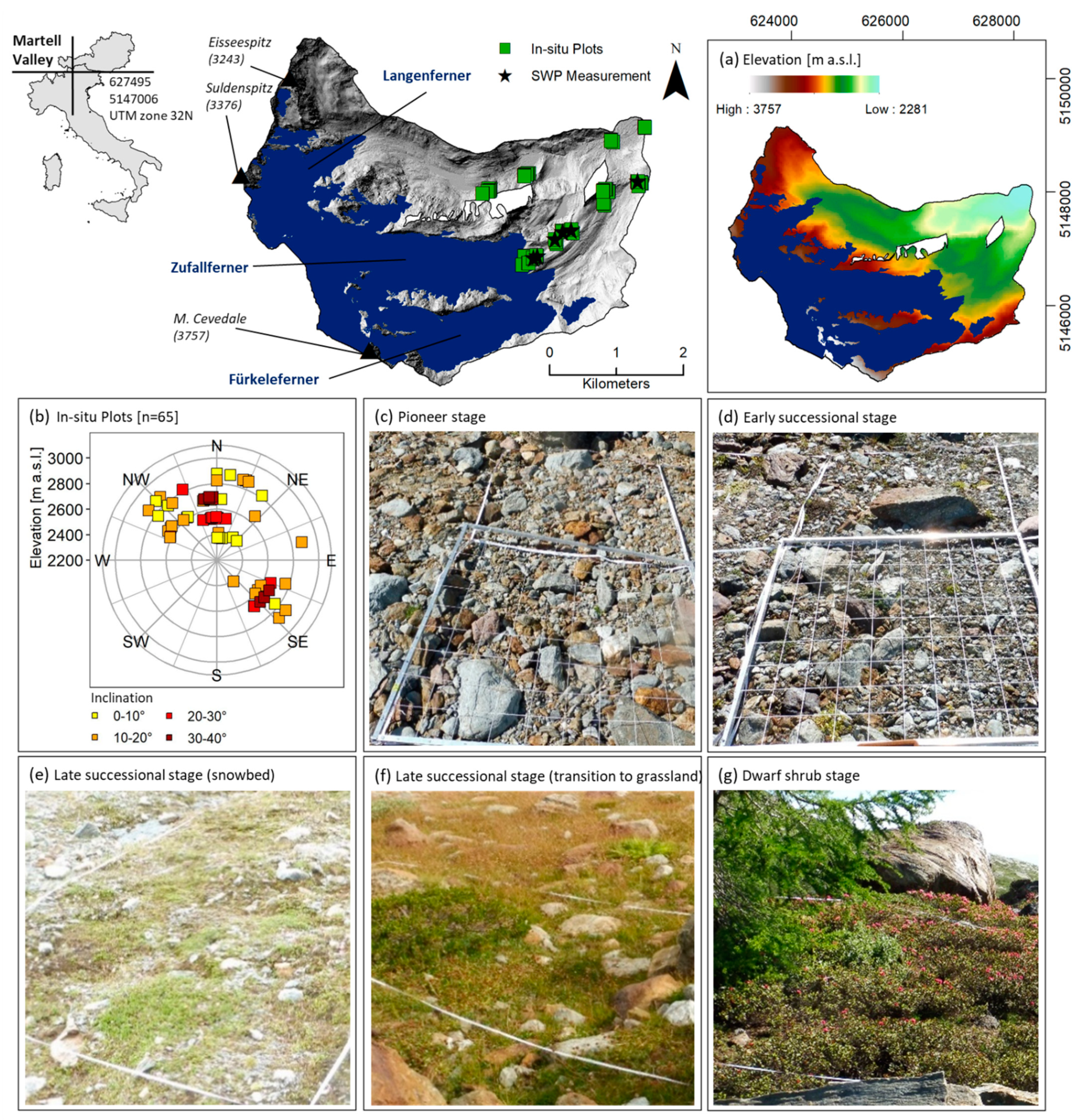
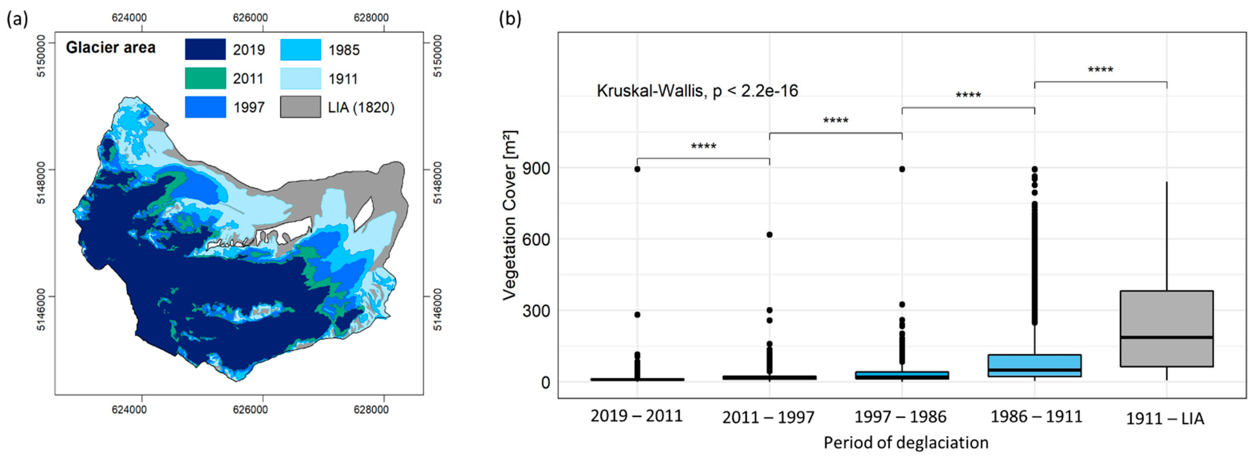
2.1. Study Area

Fürkeleferner (Vedretta della Forcola), Zufallferner (Vedretta del Cevedale) and Langenferner (Vedretta Lunga) are valley glaciers located at the head of upper Martell valley (46.46°N, 10.64°E; Figure 1) in the Vinschgau/Autonomous Province of Bozen/Bolzano, South Tyrol (Eastern Italian Alps). The high mountain range of the Ortles-Cevedale group surrounds the watershed of the once-contiguous glaciers, which are situated within a transition zone between a climatic system under the influence of the Mediterranean climate to the south and the drier conditions in the inner-Alpine zone to the north [67].
During the LIA, glaciers advanced for several hundred years. Dendroclimatic reconstructions from the Italian Central Alps revealed the lowest temperature values for the period 1813–1821 [68] (p. 216). In this period, which is known as the coldest phase of the LIA (e.g., [69]), most Italian glaciers and many glaciers in the Western Alps reached their maximum Holocene extent (e.g., [70,71,72]).
In the study area, the still well-preserved moraine walls bear witness to this maximum glacier extent at around 1820. The period after 1821 is characterized by an increase in air temperature, which is particularly noticeable after 1850, the end of the LIA [68]. Between the maximum glacier extent and today, intermittent re-advances by several hundred meters were documented in the 1890s and 1980s. None of the advances reached again the LIA maximum position, so that further terminal moraine walls can be observed [66,73,74,75]. Since the mid-1980s, the study area again has been undergoing a strong and accelerating glacier retreat with a consequent enlargement of the glacier forelands, opening up new terrain for primary succession.

2.2. Data and Methods

2.2.1. Field Investigations and Analyses of Vegetation Cover

A total of 65 vegetation plots with aspects between north-west and south-east and different inclination were established on ground and lateral moraines of the study area (Figure 1). Most of the plots were located at the forelands of Fürkele- and Zufallferner (n = 47, Figure 1) along an elevation gradient between 2377 m and 2881 m a.s.l. (Figure 1a).
At the Langenferner glacier foreland, which was altered several times by repeated glacier lake outburst floods until the 1890s [76,77,78], vegetation analyses (n = 18) were conducted only on lateral moraines (Figure 1). On each vegetation plot, the total vegetation cover was recorded in 5 × 2 m plots. On the youngest moraines (deglaciated between 1985 and 2019), cover was estimated in each 1 m2 subplot (in total 10 × 1 m2 per plot) with the smallest cover unit of 0.001%. On the older moraines (deglaciated between 1820 and 1985) the smallest cover unit was 0.0001% per 10 m2 plot. The 1 m2 data were converted to mean ground cover values per 10 m2 [79]. Vegetation sampling was performed in August 2019 and August 2020. Nomenclature of vascular species follows Fischer et al. [80]. Mosses and ground lichens as well as fruticose lichens were considered as species groups and not determined to species level. Only the lichen Stereocaulon alpinum and the moss Racomitrium sp. were distinguished because of their abundance, and the number of taxa were given. For each sample, plot aspect, inclination and elevation were calculated in ArcGIS 10.6.1 (Figure 1b).
Furthermore, the soil water potential (SWP) was measured continuously (interval 1 h) with MicroLog V3A (EMS Brno) at six plots of different age and elevation at the glacier forelands of Fürkele- and Zufallferner since August 2019 (Figure 1). To define the different plant communities, a nonmetric multidimensional scaling (NMDS) using the package vegan, version 2.5.6 [81] based on square root transformation of the in-situ observations and Bray-Curtis dissimilarity, was performed. Plots with no vegetation had to be excluded (n = 2) within the NMDS. Additionally, the samples were classified using the package twinspanR [82] in R [83] to confirm the NMDS groups. The cover values of the different plant communities were then used to define the thresholds to assign the area-wide model results to successional stages according to the modelled cover values.

2.2.2. Satellite Derived VIs and Vegetation Cover Modelling

The area-wide modelling of the vegetation cover is based on spectral VIs calculated from Landsat 8OLI, Landsat ETM7 and Landsat 5TM scenes between 1985 and 2019 (Table 1). Several studies confirm that time series extracted from different Landsat sensors can provide a representative picture of vegetation changes [84,85].
All remotely sensed VIs (NDVI, SAVI, MSAVI, EVI) were acquired as surface reflectance imagery from the Landsat Earth Explorer data portal managed by the USGS (http://earthexplorer.usgs.gov accessed on 3 November 2021) with a pixel (k) resolution of 30 m × 30 m, enabling direct comparison of multiple images over the same region [47,48]. Detailed information and comparisons of the bandwidths, spatial resolutions and main characteristics of the Landsat-sensors can be found directly at https://landsat.gsfc.nasa.gov/ (accessed on 3 November 2021).
In a first step, the four different VIs were tested to find the most accurate index representing the in-situ data. Since, due to the resolution, each of our in-situ plot falls entirely within a Landsat pixel, it was possible to extract the respective VI value for each vegetation plot from the images corresponding to the sampling year 2019 or 2020 (Table 1). Afterwards, a Bayesian beta regression using RStan [86] in R [83] was performed for each of the four VIs. Beta regression models are a commonly used and appropriate tool for percentage or proportional data, especially when data are not normally distributed [87]. The conditional expectation of proportional cover (μ) was modelled as a function of the (standardized) vegetation index using a logit link function:
μ = logit−1(a + B ∗ X)
where a is an intercept, B is a slope vector, X is the covariate matrix and logit−1(x) is the inverse of the log odds ratio:
logit 1 ( x ) = e x 1 + e x
We used a Beta likelihood for proportional cover; this likelihood has two shape parameters, α and β, which can be determined from the conditional expectation along with an additional dispersion parameter φ:
α = μ ∗ φ
β = (1 − μ) ∗ φ
cover ~ Beta(α, β)
The priors for the regression parameters (a, B) and for the dispersion parameter (φ) were chosen for regularization following Gelman et al. [88] for logit-scale and to keep value reasonable for standardized x as following: a ~ normal(0, 10), B ~ normal(0, 10) and phi ~ half cauchy(0, 5). Rstan samples from the joint posterior distribution using Hamiltonian Monte Carlo. We ran four simultaneous chains to assess convergence using the Gelman-Rubin diagnostic (Rhat), where values greater than one indicate a lack of convergence [89]; model convergence was also assessed visually using traceplots. All models were run for 4000 iterations per chain, with 2000 iterations discarded as warm-up samples.
To compare the different vegetation indices for their performance in predicting proportional cover we used the loo package in R [90]. The loo package emulates leave-one-out cross-validation methods, without the computational overhead of fitting large numbers of models. The primary diagnostic returned by this procedure is the expected log pointwise predictive density (elpd), which is an estimate of out-of-sample predictive accuracy and is a Bayesian analogue to commonly-used information criteria such as the Akaike Information Criterion (AIC). We compared competing models by computing the difference between each model’s elpd and the elpd of the best-fitting model: elpddiff,i = elpdmaxelpdi. A model with elpddiff = 0 is the best model in the set, models with elpddiff < 2 were considered strong models and models with elpddiff > 10 were considered poor-performing relative to the best model [91]. Finally, we computed model stacking weights [92] as an additional indicator of model performance.
In a second step, an area-wide reconstruction of the vegetation cover of the whole glacier forelands of Fürkele-, Zufall- and Langenferner was performed by predicting from the best-performing model. The first selected scene was recorded on 16 August 1986 and represents the end of the last glacier re-advance [66]. To observe the evolution of the total vegetation cover, further scenes were selected at the end of each decade. In order to track the maximum vegetation development of each year (t), the scene selection was limited to those datasets that were acquired in August showing clear skies and no snow cover in the proglacial area (Table 1). Predictions for unobserved locations were obtained using posterior predictive simulation [93], with credible intervals estimated from empirical quantiles from posterior samples. For each value, the standard error was calculated. The model output comprised the total vegetation cover (Vegcover) and the standard error of proportion for the corresponding year (t) as a raster data set with a pixel resolution (k) of 30 m × 30 m. The code of the model is available in the Supplemental Material (S1).
In order to investigate the spatio-temporal development, both the area with vegetation and the standard error were additionally converted from proportions to square meters and square kilometers, respectively. To obtain the vegetation cover for the different successional stages, each pixel of the model output was assigned to a successional stage based on the modelled cover and the thresholds obtained by the in-situ observations (see 2.2.1). The total area with vegetation for a given successional stage was calculated by summing up the vegetation cover of those pixels (k) covering the appropriate successional stage. The associated standard error was determined directly on the posterior simulations over the number of pixels covering the corresponding successional stage.
The statistical analysis of vegetation cover change is pixel-based, examining significant differences in mean vegetation cover change over time for the successional stages. By assuming a maximum Holocene glacier extent around 1820 and thus a total ice cover in the study area, the temporal dynamics of vegetation cover could be analyzed in four periods (1820–1986, 1986–1997, 1997–2011 and 2011–2019). The development of the vegetation until 1986 was directly reproduced from the data set Vegcover1986. For the other time periods, the change in vegetation cover (ΔVegcovert2-t1) was determined by subtracting the corresponding data sets, whereas t1 represents the earlier and t2 the later year of investigation. Since the time intervals of the individual observation periods are not identical, the change in vegetation cover per year (ΔVegcovert2-t1 a−1) was calculated.

2.2.3. Environmental Parameters: Temperature, Topographical Data, and Glacier Information

Understanding the spatio-temporal distribution of vegetation cover in relation to environmental parameters is essential to assess the impact of climate change in proglacial systems. Therefore, the modeled total vegetation cover was analyzed under consideration of its potential influencing factors, including temperature data, topographical parameters and glacier extent. The statistical correlations between vegetation cover and the different environmental parameters were determined with the Kruskal-Wallis test and the t-test.
The relation between primary succession and temperature, as a key climate factor for controlling the colonization, plant growth and community development in high mountain areas, was determined using the 20CRv3—20th Century Reanalysis version 3 data (1836–2015) provided by the National Oceanic and Atmospheric Administration (NOAA) [94,95]. The data were extracted by a bilinear interpolation to the coordinates of 46.48°N and 10.69°E. The significance of the trend was tested with the Mann-Kendall test and the t-test using the statistical software HyStat [96]. Since the spatial resolution of the data is 1° × 1°, the time series gives an insight into the long-term climate trend, but is not suitable for reflecting the spatial temperature variability. Thus, area-wide local analyses of mean June-July-August (JJA) temperature of the investigated years (2019, 2011, 1997 and 1986) were carried out as important control factors for energy and duration of vegetation development. The mean daily surface temperature of the study area was interpolated with the meteorological sub-model of the fully distributed hydrological model WaSiM [97] on a 25 m × 25 m grid resolution. Since the temperature data availability of high elevation stations (>2900 m a.s.l.) is very limited prior to 2012, the temperature lapse rate was first determined for the period 2012 to 2020. Based on nine temperature time series (S2 in Table S1 of the Supplemental Material), ranging from 1720 to 3328 m a.s.l., an annual mean temperature lapse rate of −0.0048 K/m was determined with the elevation dependent regression method of WaSiM. This constant temperature lapse rate was applied to the temperature observation of the station Zufritt (upper Martell Valley; 46.51°N, 10.73°E; 1851 m a.s.l.), neglecting any seasonal or long-term changes of the lapse rate throughout the period 1986–2019. The simulated surface temperature could not be adjusted for topographical shadowing due to a lack of solar radiation data. The temperature simulation was available in a daily time step and interpolated to a spatial grid resolution of 25 m × 25 m. From the daily temperature, the mean temperature for June, July and August was calculated for each pixel and resampled to a grid size of 30 m × 30 m using bilinear interpolation. The temperature time series of Zufritt station was also quality tested with the statistical software HyStat [96]. The results show an inhomogeneity in the median and mean of the time series using the Kruskal-Wallis-Test and t-Test, a significant change point in April 1988 using the Bernier and Pettit method, as well as a significant increasing trend following the t-Test for the slope coefficient and the Mann-Kendall test.
Topographical information was obtained from an Airborne Laser Scanning (ALS) derived Digital Terrain Model (DTM). The ALS point cloud was recorded during a flight campaign on 9 August, 2019 with the VP1 (VuxSys LR) mobile laser scanner (Riegl.com) mounted on an Airbus AS350 B3 helicopter and has an average point density of 10 pt/m2. The points were used to calculate a DTM with a resolution of 1 × 1 m, where the height value within a raster cell was determined by moving planes interpolation. Furthermore, areal images were acquired during the flight and processed to obtain an orthophoto of the study area.
In order to investigate the relationship between glacier retreat, and thus the temporal development of proglacial area, and the vegetation cover, area-wide glacier information was required. For this study, the glacier outlines for 2019, 2011, 1997 and 1985 and the LIA maximum extent were compiled based on (i) ALS data, (ii) areal images, (iii) historical maps and (iiii) field mapping (Table 2). The glacier extent of 2019 was derived from the ALS campaign described above. The inventory of 2011 was compiled from ALS data by Galos et al. [98] and revised for this study based on the original data. The scanned aerial images of 1985 were oriented and calibrated in a bundle block adjustment [99] using ground control points. Afterwards, a DTM was derived by image matching and used to create an orthophoto mosaic of pixel size 75 cm. Subsequently, the inventory, as well as those of 2019 and 2011, was digitized manually following the approach of Abermann et al. [100]. The glacier extent of 1997 was adopted from the Glacier Inventory South Tyrol (Hydrological Office of the Autonomous Province of Bozen/Bolzano, South Tyrol). The 1911 outlines were derived from the 4th Federal Survey Map (1:25.000). The scanned map was georeferenced (ETRS89, UTM 32) with up to 50 referencing points spread over the upper Martell valley. The referencing points were chosen by following the approach of Heller [101]. The LIA inventory was digitized manually by mapping moraines based on ALS data under consideration of orthophotos, the maps of Stötter [74] and Viebahn [75] and field observations. The glacier area resulted from the manually mapped polygons for each point of time. The area change, and thus the development of the proglacial area, was determined by overlaying of the polygon shapefiles of the respective years.

3. Results

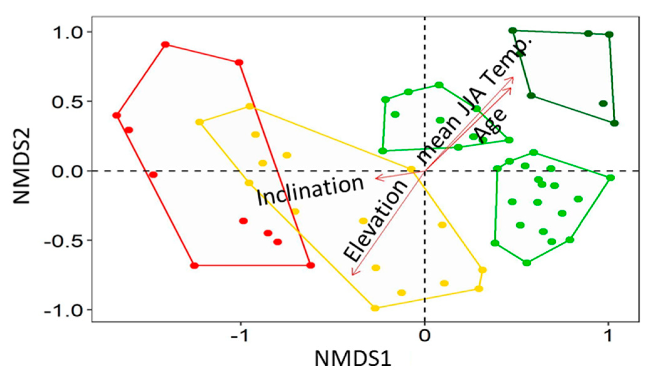
3.1. Field Investigations of the Vegetation Cover at the Glacier Forelands

In the proglacial area of Fürkele-, Zufall- and Langenferner, overall 136 vascular plants and 11 fruticose lichens and mosses were recorded. The gradual change in species composition between plots along the chronosequence allowed a discrimination of successional stages (Figure 2), which clearly differed in their mean vegetation cover. The pioneer stage (Figure 1c) had an extremely low vegetation cover (0.0006–0.9% per 10 m2, mean = 0.33%) with a minimum of three species and a maximum of 15 species per plot. The early successional stage (Figure 1d) had distinctly higher cover values (1–15% per 10 m2 mean = 7.31%) than the pioneer stage. Here, the moss Racomitrium sp. and the lichen Stereocaulon alpinum as well as dwarf shrubs occurred for the first time. The number of species ranged between 9 (minimum) and 31 (maximum) per plot. The late successional stage had a cover between 15 and 60% per 10 m2 (mean = 49.95%) with 22 to 40 species. This stage could be differentiated into a community indicating a snowbed community as well as a transitional community towards an alpine grassland (Figure 1e,f). As the two communities had similar cover values, for this study only one late successional stage was defined. In the dwarf shrub stage (Figure 1g), the cover was between 60 and 81% per 10 m2 (mean = 70.8%) with a species number ranging from 18 to 44. By following these field investigations, the thresholds of vegetation cover for the successional stages were less than 1% for the pioneer stage, 1 to 14.9% for the early successional stage, 15–59.9% for the late successional stages and more than 60% for the dwarf shrub stage (Table 3).

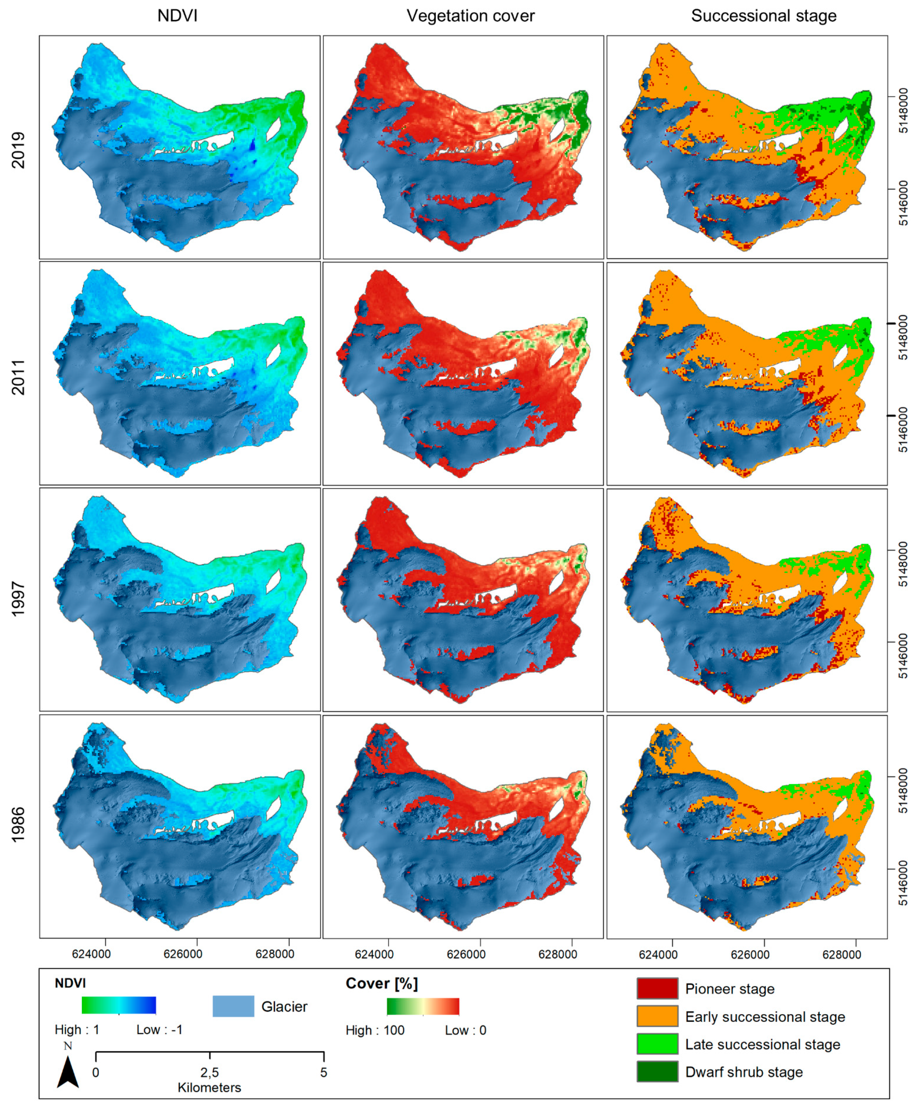
3.2. Vegetation Cover Modelling Based on Satellite Derived VIs

Both elpddiff and stacking weights showed that the model using NDVI as a predictor had the greatest support (Table 4a). Traceplots indicated the chains mixed well and Rhat was equal to one for all parameters, indicating no convergence issues (Table 4b). Table 4b displays the means for the intercept (a) −1.17, with a 95% credible interval CI = (−1.39, −0.95) and for the slope parameter B 1.51, with a 95% CI (1.26, 1.74). The effective sample size (n_eff), which is smaller than the number of iterations, is an estimate of the number of uncorrelated posterior samples. Because the model using NDVI was clearly superior in describing the in-situ observations, the area-wide modelling of the total vegetation cover was based on the NDVI. The comparison of the NDVI-based predicted vegetation cover and the in-situ vegetation cover illustrated that more than 95% of the points contrasting the in-situ cover and the modelled cover describe the course of the median of the model prediction (black line) well (Figure 3a). In less than 5% (3 plots; Figure 3a, yellow points), the modelled cover differs remarkably, with the in-situ cover being higher in all three cases. These three plots differed from the others by their higher values of lichens (mainly Stereocaulon alpinum) and mosses (mainly Racomitrium sp.) (Figure 3b). While in all other plots a maximum cover of lichens of 19.5% (mean 1.88%, mainly no Stereocaulon alpinum and ground lichens) and a maximum cover of mosses of 50% (mean 7.56%, mainly no Racomitrium sp.) were observed, higher values—a maximum cover of lichens of 15% (mean 10.5%, mainly ground lichens and Stereocaulon alpinum) and a maximum cover of mosses of 57% (mean 31.83%, mainly Racomitrium sp.)—were detected in the three outliers. The first of these plots had a high cover of ground lichens (15%), the second showed a high cover of ground lichens (10%) in combination with a high cover of Racomitrium sp. (15%) and the third a combination of 30% Racomitrium sp. and 7% Stereocaulon alpinum and ground lichens 1%. The results of the area-wide vegetation modelling for the four investigated years are illustrated in Figure 4.

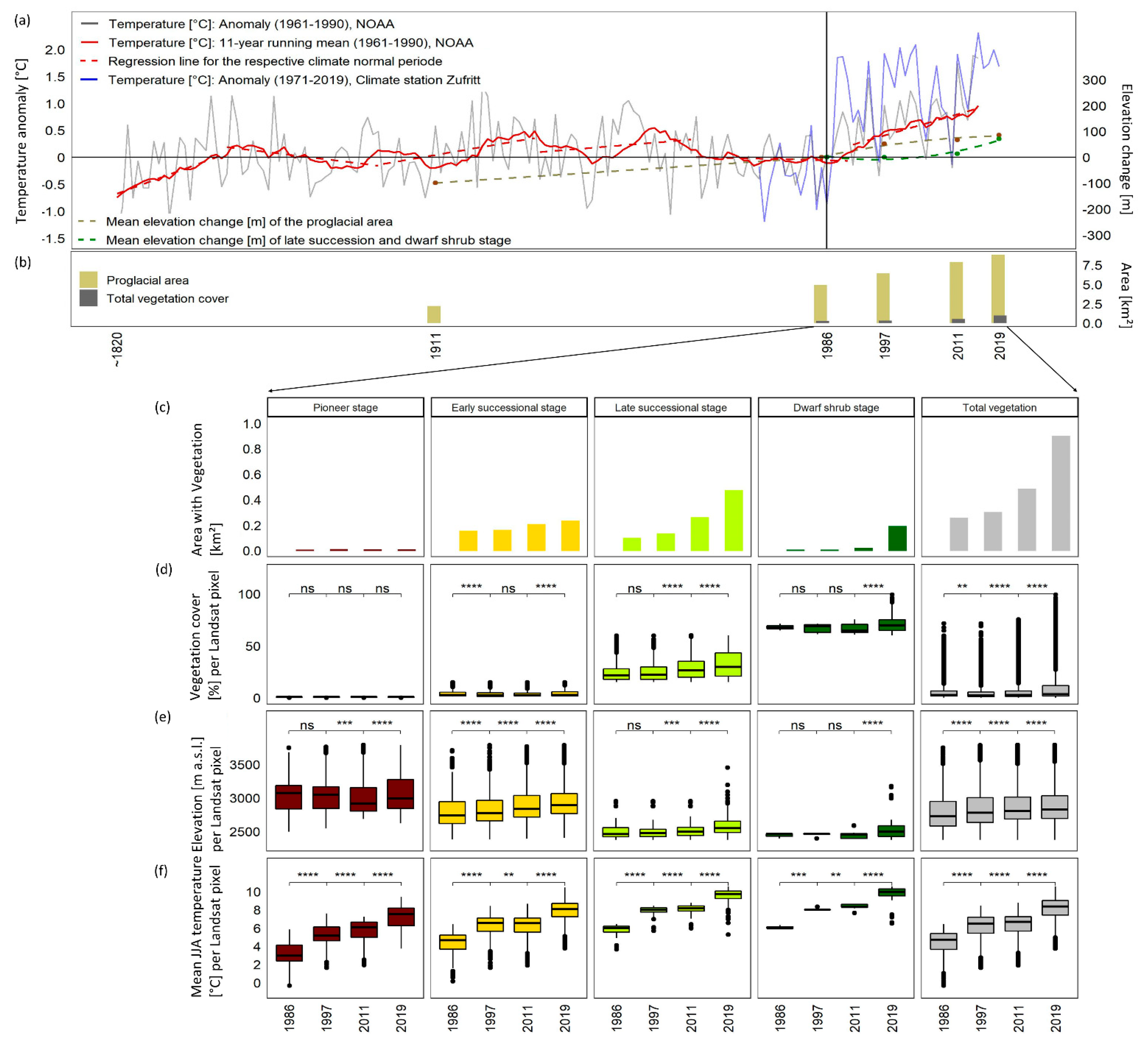
3.3. Temperature Development, Glacier Retreat and Spatio-Temporal Trends of Vegetation Cover

The analyses of the long-term temperature time series (20CRv3—20th Century Re-analysis version 3 data; NOAA) showed a significantly positive temperature trend for the study area, with an increase of +1.2 °C since the beginning of the observation period (1836–1865 in comparison to 1986–2015; 30 year period). An enhanced positive trend was observed from the 1980s to the 2000s with an increase of +0.4 ± 0.1 °C/decade, which is consistent with the temperature increase from the station data (0.46 °C/decade; weather station Zufritt; see Table S1 of the Supplemental Material). In comparison to the mean annual temperatures, the mean JJA temperature revealed a higher trend with +0.7 °C/decade for the same period (weather station Zufritt) (Figure 5a). This climatic development caused a massive glacier retreat in the study area. Since the maximum Holocene extent at about 1820 (14.2 km2), the glacier area has decreased to 6.1 km2 in 2019, which corresponds to a loss of 56.9%. The decrease of the glacier area led to a constant enlargement of the glacier foreland over the observation period (Figure 5b, Table 5). Deglaciation and the resulting age of freshly exposed glacio-fluvial sediments showed a statistically highly significant influence on the degree of vegetation cover (Figure 6), with areas that became ice-free before 1911 having on average 25% higher cover values than those that deglaciated after 2011.
In general, the total vegetation cover showed an increase in area for all four observed years and has risen from 0.25 km2 in 1986 to a total of 0.3 km2, 0.48 km2 and 0.90 km2 in 1997, 2011 and 2019, respectively (Figure 5c, Table 5a). However, percentage analyses revealed that the amount of proglacial area change relative to the preceding year was decelerating, while that of total vegetation was accelerating (Table 5b). Until 1997, the percentage of proglacial area developed faster than the vegetation cover, leading to a decrease of the percentage proglacial vegetation cover from 5.6% in 1986 (proglacial area: 4.5 km2) to 5.1% (proglacial area: 5.9 km2) in 1997. From this point onwards, a trend reversal and thus a constant increase in total vegetation cover of 6.7% in 2011 (proglacial area: 7.2 km2) and 11.2% in 2019 (proglacial area: 8.1 km2) was observed.
Although for all modelled successional stages a constant vegetation cover increase could be monitored over the whole period 1986–2019, the pioneer stage showed an area loss of 0.002 km2 from 1997 (0.007 km2) to 2011 (0.005 km2) and thus a reduction of −28.6% (Table 5b). At the same time, the early successional stage displayed an increase of 28.3%. Detailed analyses showed that from the 11.6% of the proglacial area, which was colonized by the pioneer stage with a maximum cover of 0.9% in 1997, 10.3% encroached to an early successional stage by 2011. Remarkably high cover changes were determined for the late successional stage with an area increase from 0.1 to 0.47 km2 for the entire observation period (Table 5a). However, the highest changes were observed for the dwarf shrub stage, with area increases of 0.003 km2 from 1986 to 1997 (+50%, Table 5b) and 0.015 km2 and 0.189 km2 in 2011 and 2019, respectively, resulting in percentage changes of the area in comparison to the preceding period of 400% and 1160% (Table 5b).
Figure 5d compares the mean cover values per pixel (i.e., % per Landsat pixel, 30 × 30 m) of the observed periods. Although a statistically significant increase of the mean cover values could be identified when considering the total cover, different patterns were identified for the individual succession stages. While no temporal differences were identified for the pioneer stage, the other stages showed a highly significant (p < 0.0001) increase between 2011 and 2019. In addition, the early successional stage also exhibited significant changes from 1986 to 1997; the late successional stage also from 1997 to 2011. The previously highlighted remarkable high cover changes in the dwarf shrub stage since 1997 (Table 5b) were reflected in a statistically significant mean cover change only for the period 2011–2019. The mean annual change in vegetation cover per Landsat pixel for the periods 1820 to 1986, 1986 to 1997, 1997 to 2011 and 2011 to 2019 (ΔVegcovert2-t1 a−1) showed an increase of 0.2 m2 yr−1, 0.5 m2 yr−1, 1.5 m2 yr−1 and 5.8 m2 yr−1, respectively.
The temperature lapse rate, which was determined based on temperature time series of nine weather stations, has a value of −0.0048 K/m. Figure 5a compares the temperature anomaly (1961–1990) of the long-term time series (20CRv3—20th Century Reanalysis version 3 data; NOAA; 1836–2015) with the respective elevation change based on the determined temperature gradient. By assuming a temperature increase of +0.4 ± 0.1 °C/decade since the 1980s, the isotherm must have risen by 275 ± 69 m in the study period (1986–2019). Delayed to this, an increase in the mean height of the proglacial area of 86 m (1985–2019), induced by the continuous glacier retreat, could be observed. Further, there was a statistically highly significant increase in mean elevation of total vegetation cover from 2772 m a.s.l. to 2858 m a.s.l. (86 m) between 1986 and 2019 (Figure 5e). This identical increase in mean elevation agrees well with the in-situ observations, with the first plants being found in the immediate vicinity of the glacier margin and thus on sediments that were ice-free for at most one year. Concerning vegetation with cover values exceeding 15% (late successional and dwarf shrub stage) and hence stages with high percentage of areal change (Table 5b), a mean elevation rise of 71 m was determined for the entire study period which was particularly evident between 2011 and 2019 (57 m). While the curve of the mean elevation of the proglacial area has gradually flattened during the study period, a highly significant increase in the mean elevation of the late successional and dwarf shrub stage has been observed, especially since 2011(Figure 5a). The mean elevation increase in vegetation cover corresponded with the increase in mean JJA temperature from 4.5 °C to 8.2 °C between 1986 and 2019 (Figure 5f). The mean temperature change for the total observation period showed statistically significant differences for all successional stages, with a highly significant temperature increase (p < 0.0001) of +1.7 °C (0.2 °C/year) between 2011 and 2019 for all stages.

4. Discussion

4.1. The Potential of NDVI to Model the Total Vegetation Cover in Proglacial Areas

The study combines in-situ vegetation observations and remotely sensed vegetation indices based on Landsat images to model the long-term vegetation cover development in the glacier forelands of Fürkele-, Zufall- and Langenferner. The in-situ observations discriminated four successional stages—a pioneer stage, an early successional stage, a late successional stage, and a dwarf shrub stage with mean vegetation cover values of 0.33%, 7.31%, 49.95% and 70.8%, respectively. These cover values were best represented by the NDVI. The high correlation between total vegetation cover values and NDVI has also been found in other proglacial areas of the European Alps [42], in the arctic tundra [49], as well as in areas with sub-Antarctic climate influence [34].
The area-wide vegetation cover could be reproduced well by Bayesian beta regression using RStan [86] for all four successional stages. Vegetation modelling using a Bayesian modelling approach is not known for other proglacial areas, so the model evaluation cannot be contrasted with other studies.
The comparison of the NDVI-based predicted vegetation cover and the in-situ vegetation cover showed good agreement except for three greater deviations (Figure 3a). The explanation for these noticed exceptions can be seen in the species composition of the plots. In particular, lichens (e.g., mostly Stereocaulon alpinum and ground lichens) and mosses such as Racomitrium sp. were not adequately represented in the remote sensing data due to their reflectance pattern differing from green vascular plants [102,103]. Studies from the eastern Canadian subarctic [102], the southeastern part of the Swedish mountains [103] and the western Himalayas [104] have observed different reflectance patterns for Stereocaulon paschale, S.saxatile and S. foliosum, respectively, compared to vascular plants. Further, Nayaka and Saxena [104] found that desiccation of Racomitrium subsecundum resulted in decreasing total reflectance in RED and NIR regions. Hence, in areas where Stereocaulon alpinum and mosses such as Racomitrium sp. are predominantly present, i.e., not in combination with substantial cover of vascular plants, the modelling results may underestimate the total vegetation cover.

4.2. Trends of Temperature, Glacier Retreat and Vegetation Cover

The annual temperature trend, showing an average warming rate of +0.4 ± 0.1 °C/decade for the study area over the last decades (1980s–2000s), is reflecting the global warming rate of surface air temperature in the European Alps of +0.3 ± 0.2 °C [1] and the increase of +0.5 °C per decade published by Carturan et al. [105] for the Careser dam weather station (Ortles-Cevedale group/Eastern Italian Alps). The positive temperature trend is also present in another highly resolved gridded temperature data set of South Tyrol covering the period 1980–2018 [106].
An obvious evidence for this warming trend is the massive retreat of glaciers [1,107,108,109]. Through the exchange of both energy and matter with the atmosphere, the meteorological conditions influence the glacier mass balance and translate it–in dependency of the response time–into changes of the glacier geometry [110]. Since the LIA, the total glacier area within our study area decreased by approximately 57% (LIA–2019), which agrees well with the published loss of 56% (LIA–2012) in the Austrian Alps [111] and the slightly higher values of 61.9% reported by Knoll et al. [112] for the Ortles-Cevedale group (LIA–2006). Further, the area loss of 23.4% observed by Carturan et al. [105] for the Ortles-Cevedale group between 1987 and 2009 corresponds to the shrinkage of 27.9% (1985–2011) determined for this study.
The gradual retreat of the glaciers and the accompanying initial ecosystem development in glacier forelands were shown by statistically significant correlations in both in-situ observations and modelling results. The expanding vegetation cover in dependency of the terrain age has been reported for various proglacial areas [8,15,16,22]. Our vegetation cover reconstruction indicates a significant acceleration in mean annual vegetation cover, changing from 0.2 m2 a−1 (1820 to 1986) to 5.8 m2 a−1 per pixel (2011 to 2019), resulting in a total vegetation cover of 0.90 km2 in 2019 (approx. 11% of the proglacial area). This statistically highly significant increase (Kruskal-Wallis, p < 2.2 × 10⁻¹⁶) indicates an enhanced successional dynamic over the studied periods. In detail, the analyses showed increasing dynamics of 0.5 m2 yr−1, 1.5 m2 yr−1 and 5.8 m2 yr−1 for the periods 1986 to 1997, 1997 to 2011 and 2011 to 2019, respectively. Our results confirm the findings of numerous studies, demonstrating rising vegetation cover at plot level [9] and area-wide [60,113] since the late 1980s. While accelerated successional dynamics have been clearly evident since 1986, the analyses for the time before 1986 yield an average value of 0.2 m2 yr−1 for a period of 166 years. As this period was characterized by variable glacial retreats and advances as well as successional dynamics, the value can only be considered as a rough estimate.
Interestingly, the total vegetation cover of all successional stages increased constantly over the monitored periods, while only in the pioneer stage a decrease in vegetation cover was evident between 1997 and 2011. At the same time, a high positive percentage change in the early successional was identified. It can therefore be assumed that the decrease in pioneer area between 1997 and 2011 can be explained by the transition to an early successional stage. In general, the increase in species richness on mountain summits due to climate change has been reported by various studies from the European Alps [114,115]. The climate-driven enhancement of species richness also leads to a higher vegetation cover in glacier forelands in the long term, which has been shown by a positive linear correlation between species cover and number in the Southern and Central European Alps [116]. Although species numbers were not shown in this study, it can be assumed that cover changes mainly occurred due to successional processes of species enrichment together with substantial growth of the species involved, revealing a landscape evolution characterized by the transition from pioneer stages with lower species number toward a grassland or a dwarf shrub stage with higher biomass (e.g., [7,9,12]) and higher species number.
However, the accuracy of the temporal development of the total vegetation cover can be influenced by different satellite remote sensing systems. While some studies show that the continuity and compatibility between multi-sensor VIs is good [117], other reports indicate that vegetation observations based on multi-decadal Landsat imagery vary slightly, especially depending on vegetation cover type and season (e.g., [118,119]).
Persistence and growth of well-established large individuals in the late successional [21] and dwarf shrub stage are particularly evident in this study through the high increases of vegetation cover during the last decades, being significant for the period 2011–2019 (for the late successional stage also for 1997–2011, Table 5b). Such densification processes were presumably driven by the highly significant increase of the mean JJA temperature of +1.7 °C (2011–2019). Furthermore, the high elevation shift of vegetation cover (57 m for late successional and dwarf shrub stage) since 1997 was primarily enabled by an acceleration of successional speed due to warming in the last decades [105]. This is reflected by significantly positive correlation between total vegetation cover in 2019 and the associated mean JJA temperature in both the in-situ plots (Figure 2) and the area-wide evaluations. The results are in accordance with the increasing dwarf shrub cover found in studies from the French Alps [120], the Russian tundra [121] and Greenland [122], showing a high correlation between shrub and dwarf shrub growth and rising mean summer temperatures. Studies from the Stelvio National Park (Italian Central Alps) [123] and the Ecrins National Park (French Alps) [46] suggest that high-elevation plant communities respond quickly and flexibly to warmer and longer growing seasons. Thus, the correlation between total vegetation cover and mean JJA temperature in general, as well as the exponential development of the late successional and dwarf shrub stages, leads to the hypothesis that higher energy availability is responsible for the considerable increase in vegetation cover. Additionally, the rise in mean vegetation cover could also be attributed to seed bank development, leading to enhanced recruitment and establishment [124].
Large valley glaciers, which provide the strongest climate signals, show changes on the century scale, leading to a delayed response of glacier area change and therefore proglacial landscape development [110,125]. This is evident in the study area by the observed temperature changes and the corresponding temperature lapse rate, which is not synchronous with mean elevation shift of 86 m a.s.l. for both proglacial area and total vegetation cover (Figure 5a). However, while the change of the glacier area and thus of the expansion of glacier forelands depends on the long-term trend of the annual mass balance [125], the vegetation development is influenced by the length of the growing season and thus seasonally [123,126], enhancing plant growth if enough water is available and reproduction if the growing season is long enough. The different progression of the temporal evolution of the mean elevation of the proglacial area and the mean elevation of the late successional and dwarf shrub stages (Figure 5a), as well as the accelerated development of area with vegetation compared to proglacial area development (Table 5b), can thus be hypothesized to be related to climatic developments and the increase in summer temperature, which is on average +0.26 °C/decade higher than the annual trend (weather station Zufritt).
Even though a general greening trend was reported in the context of climate warming for many mountain ranges in the European Alps [46,127], North America [113], High Mountain Asia [128,129] and Arctic and sub-Arctic environments [130,131], some studies found transforming forces on cold-adapted plant communities and reduction of vegetation cover, most probably related to a climate-induced temperature rise and concomitant drier conditions [129,132,133]. Drought effects can probably be precluded in our study area at least for the study year 2019, as the water potential measurements have shown more than −1.6 MPa moisture (data not shown) and thus, according to Körner [134], sufficient water availability for plants was ensured. Sufficient water availability might also be responsible for an acceleration of the colonization speed. Similar to studies in glacier forelands of the Sforzellina glacier (Central Italian Alps/Italy) [15], on Jamtalferner (Silvretta/Austria), Schwarzenbergferner (Stubai/Austria), Lenksteinferner (Rieserferner/Italy) and Goldbergkees (Hohe Tauern/Austria) [22], the first colonizing plants in the study area were found already one year after deglaciation, in contrast to three to five years during the 20th century [7].

4.3. Future Dynamics in the Study Area

Since the development of glacier area can be seen as a delayed long-term effect of changing climate, the proglacial area will continue to increase, even without a rise of future temperature [135,136]. Both successional dynamics through densification processes and plant colonization in higher elevations could reduce erosion processes and thus contribute to an enhanced stabilization of the continuously exposed unconsolidated sediments in proglacial areas [25,137].
However, concerning the evolution of proglacial areas, the glacier geometry mainly controls the dynamic response characteristics [110]. Since the factors for both glacier development and plant succession are controlled by topography (e.g., slope, aspect and elevation), the results must be considered in the context of the study area. The significant changes of large-scaled spatial distribution and patterns of vegetation, as well as enhanced temporal dynamics, have a number of implications for ecological functions and landscape evolution in high mountain areas [24] with implications for the hydrosphere, lithosphere, biosphere and pedosphere [5]. In order to adequately assess this response of ecosystem development in the context of climate change, further studies need to be carried out in other glacier forelands, especially those of small or medium-sized glaciers.

5. Conclusions

Under consideration of both field investigations and satellite data (Landsat data), an area-wide reconstruction of the total vegetation by using a Bayesian beta regression model with the NDVI as predictor was identified as an excellent tool to demonstrate vegetation changes through time. We were able to show that satellite-based monitoring over a longer time period can mitigate the shortcomings of the space-for-time substitution approach, as many sites are modelled at multiple points in time instead of mapping several sites once, along a gradient of time since deglaciation.
The reasons for the observed vegetation cover change in the proglacial area of Fürkele-, Zufall- and Langenferner are hypothesised to be related to (i) the glacier retreat, as the resulting age of freshly exposed glacio-fluvial sediments showed a statistically high significant influence on the degree of vegetation cover, (ii) quite fast plant colonization of areas at higher elevations and (iii) enhanced densification processes due to higher summer temperatures.
To complement the existing research on the sensitivity and response of vegetation to climate drivers in proglacial areas, we believe that a consideration of both field investigations and NDVI are necessary to attribute the observed changes and thus accurately interpret the remotely sensed data. However, since both glacier retreat and spatial distribution of vegetation development are also controlled by topographical parameters, the results must be interpreted in the context of the study area.

Supplementary Materials

The following are available online at https://www.mdpi.com/article/10.3390/rs13214450/s1. Table S1: S2 Temperature observation stations in and around the Martell Valley.

Author Contributions

Conceptualization, B.K., K.R., C.G., B.E. and J.S.; data curation, B.K., K.R., F.H. (Florentin Hofmeister), F.H. (Florian Haas), T.H., M.P., L.P., C.R., M.H.W., B.E and J.S.; formal analysis, B.K., K.R., M.T., F.H. (Florentin Hofmeister), B.E. and J.S.; funding acquisition, C.G., B.E. and J.S.; investigation, B.K., K.R.; methodology, B.K., K.R., M.T., F.H. (Florentin Hofmeister), F.H. (Florian Haas), T.H., M.P., L.P., C.R., M.H.W., C.G., B.E. and J.S.; project administration, C.G., B.E. and J.S.; resources, C.G., B.E. and J.S.; software, B.K., K.R., M.T., F.H. (Florentin Hofmeister), F.H. (Florian Haas), T.H., M.P., L.P., C.R. and M.H.W.; supervision, M.T., C.G, B.E. and J.S.; validation, M.T., C.G., B.E. and J.S.; visualization, B.K. and K.R.; writing—original draft, B.K. and K.R.; writing—review and editing, M.T. and F.H. (Florentin Hofmeister), F.H. (Florian Haas), T.H., M.P., L.P., C.R., M.H.W., C.G., B.E. and J.S. All authors have read and agreed to the published version of the manuscript.

Funding

The study was part of a cooperation between the CryoSoil_TRANSFORM project, financially supported by the Austrian Academy of Sciences (ÖAW, project no. P7160-020-020) as part of the Earth System Sciences (ESS) research program and the SEHAG project (“Sensitivity of High Alpine Geosystems to Climate Change Since 1850”), financially supported by the German Research Foundation (DFG, project ER 905/1-1, project no. 409552118) and the Austrian Science Fund (FWF) (grant numbers: BE 1118/38-1, BE 1118/39-1, BE 1118/40-1, HA 5740/10-1, HE 5747/6-1, ER 905/1-1, DI 639/5-1, CH 981/3-1, MA 6966/4-1, LA 4426/1-1 and 4062-N29).

Data Availability Statement

Landsat satellite data and the 20th Century Reanalysis V3 data are publicly available from the Web site of the U.S. Geological Survey (https://www.usgs.gov/; 25 September 2020) and the NOAA/OAR/ESRL PSL, Boulder, Colorado, USA (https://psl.noaa.gov/data/gridded/data.20thC_ReanV3.html; 4 November 2019), respectively. The code for the Bayesian beta regression model in RStan is available in the Supplementary Material. Contact the corresponding author for further data requests.

Acknowledgments

We gratefully acknowledge the ÖAW (project no. P7160-020-020), DFG (project ER 905/1-1, project no. 409552118) and the FWF for the financial support. We would also like to acknowledge the NOAA/OAR/ESRL PSL, Boulder, Colorado, USA for providing the 20th Century Reanalysis V3 data, the Institute of Atmospheric and Cryospheric Sciences—University of Innsbruck for providing the meteorological data and the USGS for providing the Satellite data. Further, we thank the Autonomous Province of Bozen/Bolzano, South Tyrol (Geoportal Alto Adige) for providing the historical images 1985 and the Hydrol. Office of the Autonomous Province of Bozen /Bolzano, South Tyrol for the Glacier Inventory of 1997. We acknowledge the MALS project (MALS—Multitemporal Laserscanning Südtirol; granted by: Autonomous Province of Bozen/Bolzano, South Tyrol, Amt für Hochschulförderung, 2011–2014) for providing the DTM of 2011 and the Austrian Federal Office of Surveying and Metrology (BEV, Austria, Vienna) for providing the map of the 4th Federal survey. We thank the Stelvio National Park for the permission to conduct the vegetation surveys, and the anonymous reviewers for valuable comments on the manuscript.

Conflicts of Interest

The authors declare no conflict of interest.

References

  1. Hock, R.; Rasul, G.; Adler, C.; Cáceres, B.; Gruber, S.; Hirabayashi, Y.; Jackson, M.; Kääb, A.; Kang, S.; Kutuzov, S.; et al. High Mountain Areas. In IPCC Special Report on the Ocean and Cryosphere in a Changing Climate; Pörtner, H.-O., Roberts, D.C., Masson-Delmotte, V., Zhai, P., Tignor, M., Poloczanska, E., Mintenbeck, K., Alegría, A., Nicolai, M., Okem, A., et al., Eds.; Cambridge University Press: Cambridge, UK, 2019; pp. 131–202. [Google Scholar]
  2. Paul, F.; Maisch, M.; Kellenberger, T.; Haeberli, W. Rapid disintegration of Alpine glaciers observed with satellite data. Geophys. Res. Lett. 2004, 31, L21402. [Google Scholar] [CrossRef] [Green Version]
  3. Zemp, M.; Haeberli, W.; Hoelzle, M.; Paul, F. Alpine glaciers to disappear within decades? Geophys. Res. Lett. 2006, 33, L13504. [Google Scholar] [CrossRef] [Green Version]
  4. Grove, J.M. Little Ice Ages: Ancient and Modern; Routledge: London, UK, 2004. [Google Scholar]
  5. Heckmann, T.; Morche, D. (Eds.) Geomorphology of Proglacial Systems: Landform and Sediment Dynamics in Recently Deglaciated Alpine Landscapes; Springer International Publishing: Cham, Switzerland, 2019; ISBN 9783319941844. [Google Scholar]
  6. Andreis, C.; Caccianiga, M.; Cerabolini, B. Vegetation and environmental factors during primary succession on glacier forelands: Some outlines from the Italian Alps. Plant Biosyst.-Int. J. Deal. All Asp. Plant Biol. 2001, 135, 295–310. [Google Scholar] [CrossRef]
  7. Raffl, C.; Mallaun, M.; Mayer, R.; Erschbamer, B. Vegetation succession pattern and diversity changes in a glacier valley, Central Alps, Austria. Arct. Antarct. Alp. Res. 2006, 38, 421–428. [Google Scholar] [CrossRef] [Green Version]
  8. Erschbamer, B.; Niederfriniger Schlag, R.; Winkler, E. Colonization processes on a central Alpine glacier foreland. J. Veg. Sci. 2008, 19, 855–862. [Google Scholar] [CrossRef]
  9. Fickert, T. Glacier forelands-unique field laboratories for the study of primary succession of plants. In Glaciers Evolution in a Changing World; Godone, D., Ed.; IntechOpen: London, UK, 2017; pp. 125–146. [Google Scholar]
  10. Losapio, G.; Cerabolini, B.E.L.; Maffioletti, C.; Tampucci, D.; Gobbi, M.; Caccianiga, M. The consequences of glacier retreat are uneven between plant species. Front. Ecol. Evol. 2021, 8, 520. [Google Scholar] [CrossRef]
  11. Frenot, Y.; Gloaguen, J.; Cannavacciuolo, M.; Bellido, A. Primary succession on glacier forelands in the subantarctic Kerguelen Islands. J. Veg. Sci. 1998, 9, 75–84. [Google Scholar] [CrossRef]
  12. Rydgren, K.; Halvorsen, R.; Töpper, J.P.; Njøs, J.M. Glacier foreland succession and the fading effect of terrain age. J. Veg. Sci. 2014, 25, 1367–1380. [Google Scholar] [CrossRef]
  13. Matthews, J.A. The Ecology of Recently-Deglaciated Terrain: A Geoecological Approach to Glacier Forelands; Cambridge University Press: Cambridge, UK, 1992; ISBN 9780521361095. [Google Scholar]
  14. Foster, B.L.; Tilman, D. Dynamic and static views of succession: Testing the descriptive power of the chronosequence approach. Plant Ecol. 2000, 146, 1–10. [Google Scholar] [CrossRef]
  15. Cannone, N.; Diolaiuti, G.; Guglielmin, M.; Smiraglia, C. Accelerating climate change impacts on alpine glacier forefield ecosystems in the European Alps. Ecol. Appl. 2008, 18, 637–648. [Google Scholar] [CrossRef] [Green Version]
  16. Schumann, K.; Gewolf, S.; Tackenberg, O. Factors affecting primary succession of glacier foreland vegetation in the European Alps. Alp. Bot. 2016, 126, 105–117. [Google Scholar] [CrossRef]
  17. Franzén, M.; Dieker, P.; Schrader, J.; Helm, A. Rapid plant colonization of the forelands of a vanishing glacier is strongly associated with species traits. Arct. Antarct. Alp. Res. 2019, 51, 366–378. [Google Scholar] [CrossRef] [Green Version]
  18. Egli, M.; Wernli, M.; Kneisel, C.; Haeberli, W. Melting glaciers and soil development in the proglacial area Morteratsch (Swiss Alps): I. Soil type chronosequence. Arct. Antarct. Alp. Res. 2006, 38, 499–509. [Google Scholar] [CrossRef] [Green Version]
  19. Kaufmann, R. Glacier Foreland Colonisation: Distinguishing between Short-Term and Long-Term Effects of Climate Change. Oecologia 2002, 130, 470–475. [Google Scholar] [CrossRef]
  20. Tscherko, D.; Rustemeier, J.; Richter, A.; Wanek, W.; Kandeler, E. Functional diversity of the soil microflora in primary succession across two glacier forelands in the Central Alps. Eur. J. Soil Sci. 2003, 54, 685–696. [Google Scholar] [CrossRef]
  21. Erschbamer, B.; Caccianiga, M.S. Glacier Forelands: Lessons of Plant Population and Community Development. In Progress in Botany Vol. 78; Cánovas, F.M., Lüttge, U., Matyssek, R., Eds.; Springer International Publishing: Cham, Switzerland, 2016; pp. 259–284. ISBN 978-3-319-49490-6. [Google Scholar]
  22. Fickert, T. Common Patterns and Diverging Trajectories in Primary Succession of Plants in Eastern Alpine Glacier Forelands. Diversity 2020, 12, 191. [Google Scholar] [CrossRef]
  23. Walker, L.R.; Wardle, D.A.; Bardgett, R.D.; Clarkson, B.D. The use of chronosequences in studies of ecological succession and soil development. J. Ecol. 2010, 98, 725–736. [Google Scholar] [CrossRef]
  24. Marston, R.A. Geomorphology and vegetation on hillslopes: Interactions, dependencies, and feedback loops. Geomorphology 2010, 116, 206–217. [Google Scholar] [CrossRef]
  25. Eichel, J.; Draebing, D.; Meyer, N. From active to stable: Paraglacial transition of Alpine lateral moraine slopes. Land Degrad. Dev. 2018, 29, 4158–4172. [Google Scholar] [CrossRef]
  26. Bayle, A. A recent history of deglaciation and vegetation establishment in a contrasted geomorphological context, Glacier Blanc, French Alps. J. Maps 2020, 16, 766–775. [Google Scholar] [CrossRef]
  27. Gottfried, M.; Pauli, H.; Futschik, A.; Akhalkatsi, M.; Barančok, P.; Benito Alonso, J.L.; Coldea, G.; Dick, J.; Erschbamer, B.; Fernández Calzado, M.R.; et al. Continent-wide response of mountain vegetation to climate change. Nat. Clim. Chang. 2012, 2, 111–115. [Google Scholar] [CrossRef]
  28. Grabherr, G.; Gottfried, M.; Pauli, H. Climate Change Impacts in Alpine Environments. Geogr. Compass 2010, 4, 1133–1153. [Google Scholar] [CrossRef] [Green Version]
  29. Verrall, B.; Pickering, C.M. Alpine vegetation in the context of climate change: A global review of past research and future directions. Sci. Total Environ. 2020, 748, 141344. [Google Scholar] [PubMed]
  30. Warren, R.; Price, J.; Fischlin, A.; de la Nava Santos, S.; Midgley, G. Increasing impacts of climate change upon ecosystems with increasing global mean temperature rise. Clim. Chang. 2011, 106, 141–177. [Google Scholar] [CrossRef]
  31. Brondizio, E.S.; Settele, J.; Diaz, S.; Ngo, H.T. (Eds.) Global Assessment Report on Biodiversity and Ecosystem Services of the Intergovernmental Science-Policy Platform on Biodiversity and Ecosystem Services. IPBES Secr. Bonn Ger. 2019, 1148. [Google Scholar] [CrossRef]
  32. IPCC. Global Warming of 1.5 °C; An IPCC Special Report on the Impacts of Global Warming of 1.5 °C above Pre-industrial Levels and Related Global Greenhouse Gas Emission Pathways, in the Context of Strengthening the Global Response to the Threat of Climate Change, Sustainable Development, and Efforts to Eradicate Poverty; IPCC: Geneva, Switzerland, 2018; p. 630. [Google Scholar]
  33. König, M.; Winther, J.-G.; Isaksson, E. Measuring snow and glacier ice properties from satellite. Rev. Geophys. 2001, 39, 1–27. [Google Scholar] [CrossRef]
  34. Robin, M.; Chapuis, J.-L.; Lebouvier, M. Remote sensing of vegetation cover change in islands of the Kerguelen archipelago. Polar Biol. 2011, 34, 1689–1700. [Google Scholar] [CrossRef]
  35. Raynolds, M.K.; Walker, D.A.; Verbyla, D.; Munger, C.A. Patterns of Change within a Tundra Landscape: 22-year Landsat NDVI Trends in an Area of the Northern Foothills of the Brooks Range, Alaska. Arct. Antarct. Alp. Res. 2013, 45, 249–260. [Google Scholar] [CrossRef] [Green Version]
  36. Xue, J.; Su, B. Significant remote sensing vegetation indices: A review of developments and applications. J. Sens. 2017, 2017, 1353691. [Google Scholar] [CrossRef] [Green Version]
  37. Reed, B.; Brown, J.F.; VanderZee, D.; Loveland, T.R.; Ohlen, D.O. Measuring Phenological Variability From Satellite Imagery. J. Veg. Sci. 1994, 5, 703–714. [Google Scholar] [CrossRef]
  38. Rouse, J.W., Jr.; Haas, R.H.; Schell, J.A.; Deering, D.W. Monitoring vegetation systems in the great Plains with Erts. NASA Spec. Publ. 1974, 351, 309. [Google Scholar]
  39. Tucker, C.J. Red and photographic infrared linear combinations for monitoring vegetation. Remote Sens. Environ. 1979, 8, 127–150. [Google Scholar] [CrossRef] [Green Version]
  40. Bannari, A.; Morin, D.; Bonn, F.; Huete, A.R. A review of vegetation indices. Remote Sens. Rev. 1995, 13, 95–120. [Google Scholar] [CrossRef]
  41. Levin, N.; Shmida, A.; Levanoni, O.; Tamari, H.; Kark, S. Predicting mountain plant richness and rarity from space using satellite-derived vegetation indices. Divers. Distrib. 2007, 13, 692–703. [Google Scholar] [CrossRef]
  42. Fischer, A.; Fickert, T.; Schwaizer, G.; Patzelt, G.; Groß, G. Vegetation dynamics in Alpine glacier forelands tackled from space. Sci. Rep. 2019, 9, 13918. [Google Scholar] [CrossRef] [PubMed] [Green Version]
  43. Kerr, J.T.; Ostrovsky, M. From space to species: Ecological applications for remote sensing. Trends Ecol. Evol. 2003, 18, 299–305. [Google Scholar] [CrossRef]
  44. Cohen, W.B.; Goward, S.N. Landsat’s Role in Ecological Applications of Remote Sensing. BioScience 2004, 54, 535–545. [Google Scholar] [CrossRef]
  45. Pettorelli, N.; Vik, J.O.; Mysterud, A.; Gaillard, J.-M.; Tucker, C.J.; Stenseth, N.C. Using the satellite-derived NDVI to assess ecological responses to environmental change. Trends Ecol. Evol. 2005, 20, 503–510. [Google Scholar] [CrossRef]
  46. Carlson, B.Z.; Corona, M.C.; Dentant, C.; Bonet, R.; Thuiller, W.; Choler, P. Observed long-term greening of alpine vegetation—A case study in the French Alps. Environ. Res. Lett. 2017, 12, 114006. [Google Scholar] [CrossRef]
  47. Masek, J.G.; Vermote, E.F.; Saleous, N.E.; Wolfe, R.; Hall, F.G.; Huemmrich, K.F.; Gao, F.; Kutler, J.; Lim, T.K. A Landsat surface reflectance dataset for North America, 1990–2000. IEEE Geosci. Remote Sens. Lett. 2006, 3, 68–72. [Google Scholar] [CrossRef]
  48. Vermote, E.; Justice, C.; Claverie, M.; Franch, B. Preliminary analysis of the performance of the Landsat 8/OLI land surface reflectance product. Remote Sens. Environ. 2016, 185, 46–56. [Google Scholar] [CrossRef]
  49. Laidler, G.J.; Treitz, P.M.; Atkinson, D.M. Remote sensing of arctic vegetation: Relations between the NDVI, spatial resolution and vegetation cover on Boothia Peninsula, Nunavut. Arctic 2008, 61, 1–13. [Google Scholar] [CrossRef] [Green Version]
  50. Walker, D.A.; Epstein, H.E.; Raynolds, M.K.; Kuss, P.; Kopecky, M.A.; Frost, G.V.; Daniëls, F.J.A.; Leibman, M.O.; Moskalenko, N.G.; Matyshak, G.V. Environment, vegetation and greenness (NDVI) along the North America and Eurasia Arctic transects. Environ. Res. Lett. 2012, 7, 15504. [Google Scholar] [CrossRef] [Green Version]
  51. Riihimäki, H.; Luoto, M.; Heiskanen, J. Estimating fractional cover of tundra vegetation at multiple scales using unmanned aerial systems and optical satellite data. Remote Sens. Environ. 2019, 224, 119–132. [Google Scholar] [CrossRef]
  52. Huete, A.R. A soil-adjusted vegetation index (SAVI). Remote Sens. Environ. 1988, 25, 295–309. [Google Scholar] [CrossRef]
  53. Qi, J.; Chehbouni, A.; Huete, A.R.; Kerr, Y.H.; Sorooshian, S. A modified soil adjusted vegetation index. Remote Sens. Environ. 1994, 48, 119–126. [Google Scholar] [CrossRef]
  54. Liu, H.Q.; Huete, A. A feedback based modification of the NDVI to minimize canopy background and atmospheric noise. IEEE Trans. Geosci. Remote Sens. 1995, 33, 457–465. [Google Scholar] [CrossRef]
  55. Purevdorj, T.S.; Tateishi, R.; Ishiyama, T.; Honda, Y. Relationships between percent vegetation cover and vegetation indices. Int. J. Remote Sens. 1998, 19, 3519–3535. [Google Scholar] [CrossRef]
  56. Fraser, R.H.; Olthof, I.; Carrière, M.; Deschamps, A.; Pouliot, D. Detecting long-term changes to vegetation in northern Canada using the Landsat satelliteimage archive. Environ. Res. Lett. 2011, 6, 45502. [Google Scholar] [CrossRef] [Green Version]
  57. McDowell, N.G.; Coops, N.C.; Beck, P.S.A.; Chambers, J.Q.; Gangodagamage, C.; Hicke, J.A.; Huang, C.-y.; Kennedy, R.; Krofcheck, D.J.; Litvak, M.; et al. Global satellite monitoring of climate-induced vegetation disturbances. Trends Plant Sci. 2015, 20, 114–123. [Google Scholar] [CrossRef] [Green Version]
  58. Chhetri, P.K.; Thai, E. Remote sensing and geographic information systems techniques in studies on treeline ecotone dynamics. J. For. Res. 2019, 30, 1543–1553. [Google Scholar] [CrossRef]
  59. Lizaga, I.; Gaspar, L.; Quijano, L.; Dercon, G.; Navas, A. NDVI, 137Cs and nutrients for tracking soil and vegetation development on glacial landforms in the Lake Parón Catchment (Cordillera Blanca, Perú). Sci. Total Environ. 2019, 651, 250–260. [Google Scholar] [CrossRef]
  60. Alessi, N.; Wellstein, C.; Rocchini, D.; Midolo, G.; Oeggl, K.; Zerbe, S. Surface Tradeoffs and Elevational Shifts at the Largest Italian Glacier: A Thirty-Years Time Series of Remotely-Sensed Images. Remote Sens. 2021, 13, 134. [Google Scholar] [CrossRef]
  61. Guisan, A.; Zimmermann, N.E. Predictive habitat distribution models in ecology. Ecol. Model. 2000, 135, 147–186. [Google Scholar] [CrossRef]
  62. Ellison, A.M. Bayesian inference in ecology. Ecol. Lett. 2004, 7, 509–520. [Google Scholar] [CrossRef]
  63. Camac, J.S.; Williams, R.J.; Wahren, C.-H.; Jarrad, F.; Hoffmann, A.A.; Vesk, P.A. Modeling rates of life form cover change in burned and unburned alpine heathland subject to experimental warming. Oecologia 2015, 178, 615–628. [Google Scholar] [CrossRef] [Green Version]
  64. Monnahan, C.C.; Thorson, J.T.; Branch, T.A. Faster estimation of Bayesian models in ecology using Hamiltonian Monte Carlo. Methods Ecol. Evol. 2017, 8, 339–348. [Google Scholar] [CrossRef]
  65. Myers-Smith, I.H.; Grabowski, M.M.; Thomas, H.J.D.; Angers-Blondin, S.; Daskalova, G.N.; Bjorkman, A.D.; Cunliffe, A.M.; Assmann, J.J.; Boyle, J.S.; McLeod, E. Eighteen years of ecological monitoring reveals multiple lines of evidence for tundra vegetation change. Ecol. Monogr. 2019, 89, e01351. [Google Scholar] [CrossRef] [Green Version]
  66. WGMS. Fluctuations of Glaciers Database. Available online: https://doi.org/10.5904/wgms-fog-2019-12 (accessed on 18 August 2020).
  67. Frei, C.; Schär, C. A precipitation climatology of the Alps from high-resolution rain-gauge observations. Int. J. Climatol. 1998, 18, 873–900. [Google Scholar] [CrossRef]
  68. Coppola, A.; Leonelli, G.; Salvatore, M.C.; Pelfini, M.; Baroni, C. Tree-ring-Based summer mean temperature variations in the Adamello-Presanella Group (Italian Central Alps), 1610-2008 AD. Clim. Past 2013, 9, 211–221. [Google Scholar] [CrossRef] [Green Version]
  69. Bradley, R.S.; Jonest, P.D. “Little Ice Age” summer temperature variations: Their nature and relevance to recent global warming trends. Holocene 1993, 3, 367–376. [Google Scholar] [CrossRef]
  70. Kinzl, H. Die grössten nacheiszeitlichen Gletschervorstösse in den Schweizer Alpen und in der Mont Blanc-Gruppe. Z. Gletsch. 1932, 20, 269–397. [Google Scholar]
  71. Porter, S.C. Pattern and forcing of Northern Hemisphere glacier variations during the last millennium. Quat. Res. 1986, 26, 27–48. [Google Scholar] [CrossRef]
  72. Ivy-Ochs, S.; Kerschner, H.; Maisch, M.; Christl, M.; Kubik, P.W.; Schlüchter, C. Latest Pleistocene and Holocene glacier variations in the European Alps. Quat. Sci. Rev. 2009, 28, 2137–2149. [Google Scholar] [CrossRef]
  73. Finsterwalder, S. Das Wachsen der Gletscher in der Ortlergruppe. Mitteilungen des Deutschen und Österreichischen Alpenvereins 1890, 16, 265. [Google Scholar]
  74. Stötter, J. Veränderungen der Kryosphäre in Vergangenheit und Zukunft sowie Folgeerscheinungen: Untersuchungen in ausgewählten Hochgebirgsräumen im Vinschgau (Südtirol). Habilitation Thesis, LMU, Institute of Geography, Munich, Germany, 1994. [Google Scholar]
  75. Viebahn, B. Untersuchungen zur Entwicklung des Formenschatzes im Inneren Martelltal—Grundla-ge für ein naturkundliches Informationsangebot im Nationalpark Stilfser Joch. Diploma Thesis, LMU, Institute of Geography, Munich, Germany, 1996. [Google Scholar]
  76. DÖAV. Mitteilungen des Deutschen und Österreichischen Alpenvereins; DÖAV: Innsbruck, Austria, 1891; Volume 17. [Google Scholar]
  77. DÖAV. Mitteilungen des Deutschen und Österreichischen Alpenvereins; DÖAV: Innsbruck, Austria, 1895; Volume 21. [Google Scholar]
  78. Richter, E. Der Gletscherausbruch im Martellthal und seine Wiederkehr. Mitt. Dtsch. Osterr. Alp. 1889, 15, 23. [Google Scholar]
  79. Pauli, H.; Gottfried, M.; Lamprecht, A.; Niessner, S.; Rumpf, S.; Winkler, M.; Steinbauer, K.; Grabherr, G. The GLORIA Field Manual–Standard Multi-Summit Approach, Supplementary Methods and Extra Approaches, 5th ed.; GLORIA-Coordination, Austrian Academy of Sciences & University of Natural Resources and Life Sciences: Vienna, Austria, 2015; ISBN 978-92-79-45694-7. [Google Scholar]
  80. Fischer, M.A.; Oswald, K.; Adler, W. Exkursionsflora für Österreich, Liechtenstein und Südtirol, 3rd ed.; Biologiezentrum der Oberösterreichischen Landesmuseen: Linz, Austria, 2008. [Google Scholar]
  81. Oksanen, J.; Blanchet, G.F.; Friendly, M.; Kindt, R.; Legendre, P.; McGlinn, D.; Minchin, P.R.; O’Hara, R.B.; Simpson, G.L.; Solymos, P.; et al. Package: Vegan (Version 2.5-7). 2020. Available online: https://cran.r-project.org/web/packages/vegan/vegan.pdf (accessed on 3 November 2021).
  82. Zelený, D.; Smilauer, P.; Hennekens, S.M.; Hill, M.O. Package: Twinspnar (Version 0.19). 2019.
  83. R Core Team. R: A Language and Environment for Statistical Computing; R Foundation for Statistical Computing: Vienna, Austria, 2020. [Google Scholar]
  84. Xu, D.; Guo, X. Compare NDVI Extracted from Landsat 8 Imagery with that from Landsat 7 Imagery. Am. J. Remote Sens. 2014, 2, 10–14. [Google Scholar] [CrossRef] [Green Version]
  85. Zhang, H.K.; Roy, D.P.; Yan, L.; Li, Z.; Huang, H.; Vermote, E.; Skakun, S.; Roger, J.-C. Characterization of Sentinel-2A and Landsat-8 top of atmosphere, surface, and nadir BRDF adjusted reflectance and NDVI differences. Remote Sens. Environ. 2018, 215, 482–494. [Google Scholar] [CrossRef]
  86. Stan Development Team. RStan: The R Interface to Stan; R Package Version 2.21.2. 2020. Available online: https://mc-stan.org/ (accessed on 3 November 2021).
  87. Ferrari, S.; Cribari-Neto, F. Beta Regression for Modelling Rates and Proportions. J. Appl. Stat. 2004, 31, 799–815. [Google Scholar] [CrossRef]
  88. Gelman, A.; Jakulin, A.; Pittau, M.G.; Su, Y.-S. A weakly informative default prior distribution for logistic and other regression models. Ann. Appl. Stat. 2008, 2, 1360–1383. [Google Scholar] [CrossRef]
  89. Gelman, A.; Rubin, D.B. Inference from Iterative Simulation Using Multiple Sequences. Stat. Sci. 1992, 7, 457–511. [Google Scholar] [CrossRef]
  90. Vehtari, A.; Gabry, J.; Magnusson, M.; Yao, Y.; Bürkner, P.-C.; Paananen, T. Package: Loo. Efficient Leave-One-Out Cross-Validation and WAIC for Bayesian Models; version 2.4.1. 2020. Available online: https://mc-stan.org/loo/ (accessed on 3 November 2021).
  91. Burnham, K.P.; Anderson, D.R. Model Selection and Inference: A Practical Information-Theoretic Approach, 2nd ed.; Springer: New York, NY, USA, 2002. [Google Scholar] [CrossRef] [Green Version]
  92. Yao, Y.; Vehtari, A.; Simpson, D.; Gelman, A. Using Stacking to Average Bayesian Predictive Distribution (with Discussion). Bayesian Anal. 2018, 13, 917–1003. [Google Scholar] [CrossRef]
  93. Gelman, A.; Carlin, J.; Stern, H.; Dunson, D.; Vehtari, A.; Rubin, D. Bayesian Data Analysis, 3rd ed.; Chapman and Hall/CRC: Boca Raton, FL, USA, 2013. [Google Scholar]
  94. Slivinski, L.C.; Compo, G.P.; Whitaker, J.S.; Sardeshmukh, P.D.; Giese, B.S.; McColl, C.; Allan, R.; Yin, X.; Vose, R.; Titchner, H.; et al. Towards a more reliable historical reanalysis: Improvements for version 3 of the Twentieth Century Reanalysis system. Q. J. R. Meteorol. Soc. 2019, 145, 2876–2908. [Google Scholar] [CrossRef] [Green Version]
  95. Compo, G.P.; Whitaker, J.S.; Sardeshmukh, P.D.; Matsui, N.; Allan, R.J.; Yin, X.; Gleason, B.E.; Vose, R.S.; Rutledge, G.; Bessemoulin, P.; et al. The Twentieth Century Reanalysis Project. Q. J. R. Meteorol. Soc. 2011, 137, 1–28. [Google Scholar] [CrossRef]
  96. Willems, W. HyStat, Benutzerhandbuch, s.l.: IAWG. Available online: http://www.hystat.de/default_e.htm (accessed on 19 February 2021).
  97. Schulla, J.; Jasper, K. Modell Description WaSiM (Water Balance Simulation Model). 2019. Available online: http://www.wasim.ch/downloads/doku/wasim/wasim_2007_en.pdf (accessed on 3 November 2021).
  98. Galos, S.P.; Klug, C.; Maussion, F.; Covi, F.; Nicholson, L.; Rieg, L.; Gurgiser, W.; Mölg, T.; Kaser, G. Reanalysis of a 10-year record (2004–2013) of seasonal mass balances at Langenferner/Vedretta Lunga, Ortler Alps, Italy. Cryosphere 2017, 11, 1417–1439. [Google Scholar] [CrossRef] [Green Version]
  99. McGlone, C.; Mikhail, E.; Bethel, J. (Eds.) Manual of Photogrammetry, 5th ed.; American Society for Photogrammetry and Remote Sensing: Bethesda, MD, USA, 2004; ISBN 1570830711. [Google Scholar]
  100. Abermann, J.; Fischer, A.; Lambrecht, A.; Geist, T. On the potential of very high-resolution repeat DEMs in glacial and periglacial environments. Cryosphere 2010, 4, 53–65. [Google Scholar] [CrossRef] [Green Version]
  101. Heller, A. Die Ableitung von Passpunkten aus hochauflösenden Fernerkundungsdaten (ALS und IFSAR) zur Georeferenzierung von Alpenvereinskarten. Angew. Geoinformatik 2011, 880–889. Available online: https://gispoint.de/fileadmin/user_upload/paper_gis_open/AGIT_2011/537508035.pdf (accessed on 3 November 2021).
  102. Petzold, D.E.; Goward, S.N. Reflectance spectra of subarctic lichens. Remote Sens. Environ. 1988, 24, 481–492. [Google Scholar] [CrossRef]
  103. Nordberg, M.-L.; Allard, A. A remote sensing methodology for monitoring lichen cover. Can. J. Remote Sens. 2002, 28, 262–274. [Google Scholar] [CrossRef]
  104. Nayaka, S.; Saxena, P. Physiological responses and ecological success of lichen Stereocaulon foliolosum and moss Racomitrium subsecundum growing in same habitat in Himalaya. Indian J. Fundam. Appl. Life Sci. 2014, 4, 167–179. [Google Scholar]
  105. Carturan, L.; Filippi, R.; Seppi, R.; Gabrielli, P.; Notarnicola, C.; Bertoldi, L.; Paul, F.; Rastner, P.; Cazorzi, F.; Dinale, R.; et al. Area and volume loss of the glaciers in the Ortles-Cevedale group (Eastern Italian Alps): Controls and imbalance of the remaining glaciers. Cryosphere 2013, 7, 1339–1359. [Google Scholar] [CrossRef] [Green Version]
  106. Crespi, A.; Matiu, M.; Bertoldi, G.; Petitta, M.; Zebisch, M. A high-resolution gridded dataset of daily temperature and precipitation records (1980–2018) for Trentino-South Tyrol (north-eastern Italian Alps). Earth Syst. Sci. Data 2021, 13, 2801–2818. [Google Scholar] [CrossRef]
  107. Haeberli, W.; Beniston, M. Climate Change and its Impacts on Glaciers and Permafrost in the Alps. AMBIO A J. Hum. Environ. 1998, 27, 258–265. [Google Scholar]
  108. Barry, R.G. The status of research on glaciers and global glacier recession: A review. Prog. Phys. Geogr. Earth Environ. 2006, 30, 285–306. [Google Scholar] [CrossRef]
  109. Paul, F.; Bolch, T. Glacier Changes Since the Little Ice Age. In Geomorphology of Proglacial Systems; Heckmann, T., Morche, D., Eds.; Springer: Cham, Switzerland, 2019; pp. 23–42. [Google Scholar]
  110. Haeberli, W.; Hoelzle, M.; Paul, F.; Zemp, M. Integrated monitoring of mountain glaciers as key indicators of global climate change: The European Alps. Ann. Glaciol. 2007, 46, 150–160. [Google Scholar] [CrossRef] [Green Version]
  111. Fischer, A.; Seiser, B.; Stocker Waldhuber, M.; Mitterer, C.; Abermann, J. Tracing glacier changes in Austria from the Little Ice Age to the present using a lidar-based high-resolution glacier inventory in Austria. Cryosphere 2015, 9, 753–766. [Google Scholar] [CrossRef] [Green Version]
  112. Knoll, C.; Kerschner, H.; Heller, A.; Rastner, P. A GIS-based reconstruction of Little Ice Age glacier maximum extents for South Tyrol, Italy. Trans. GIS 2009, 13, 449–463. [Google Scholar] [CrossRef]
  113. Lambert, C.B.; Resler, L.M.; Shao, Y.; Butler, D.R. Vegetation change as related to terrain factors at two glacier forefronts, Glacier National Park, Montana, USA. J. Mt. Sci. 2020, 17, 1–15. [Google Scholar] [CrossRef]
  114. Pauli, H.; Gottfried, M.; Dullinger, S.; Abdaladze, O.; Akhalkatsi, M.; Alonso, J.L.B.; Coldea, G.; Dick, J.; Erschbamer, B.; Calzado, R.F. Recent plant diversity changes on Europe’s mountain summits. Science 2012, 336, 353–355. [Google Scholar] [CrossRef] [Green Version]
  115. Steinbauer, M.J.; Grytnes, J.-A.; Jurasinski, G.; Kulonen, A.; Lenoir, J.; Pauli, H.; Rixen, C.; Winkler, M.; Bardy-Durchhalter, M.; Barni, E. Accelerated increase in plant species richness on mountain summits is linked to warming. Nature 2018, 556, 231–234. [Google Scholar] [CrossRef]
  116. Erschbamer, B.; Mallaun, M.; Unterluggauer, P. Plant diversity along altitudinal gradients in the Southern and Central Alps of South Tyrol and Trentino (Italy). Gredleriana 2006, 6, 47–68. [Google Scholar]
  117. Li, P.; Jiang, L.; Feng, Z. Cross-Comparison of Vegetation Indices Derived from Landsat-7 Enhanced Thematic Mapper Plus (ETM+) and Landsat-8 Operational Land Imager (OLI) Sensors. Remote Sens. 2014, 6, 310–329. [Google Scholar] [CrossRef] [Green Version]
  118. Ke, Y.; Im, J.; Lee, J.; Gong, H.; Ryu, Y. Characteristics of Landsat 8 OLI-derived NDVI by comparison with multiple satellite sensors and in-situ observations. Remote Sens. Environ. 2015, 164, 298–313. [Google Scholar] [CrossRef]
  119. She, X.; Zhang, L.; Cen, Y.; Wu, T.; Huang, C.; Baig, M.H.A. Comparison of the Continuity of Vegetation Indices Derived from Landsat 8 OLI and Landsat 7 ETM+ Data among Different Vegetation Types. Remote Sens. 2015, 7, 13485–13506. [Google Scholar] [CrossRef] [Green Version]
  120. Francon, L.; Corona, C.; Roussel, E.; Lopez Saez, J.; Stoffel, M. Warm summers and moderate winter precipitation boost Rhododendron ferrugineum L. growth in the Taillefer massif (French Alps). Sci. Total Environ. 2017, 586, 1020–1031. [Google Scholar] [CrossRef] [PubMed]
  121. Blok, D.; Sass-Klaassen, U.; Schaepman-Strub, G.; Heijmans, M.M.P.D.; Sauren, P.; Berendse, F. What are the main climate drivers for shrub growth in Northeastern Siberian tundra? Biogeosciences 2011, 8, 1169–1179. [Google Scholar] [CrossRef] [Green Version]
  122. Jørgensen, R.H.; Hallinger, M.; Ahlgrimm, S.; Friemel, J.; Kollmann, J.; Meilby, H. Growth response to climatic change over 120 years for Alnus viridis and Salix glauca in West Greenland. J. Veg. Sci. 2015, 26, 155–165. [Google Scholar] [CrossRef]
  123. Cannone, N.; Sgorbati, S.; Guglielmin, M. Unexpected impacts of climate change on alpine vegetation. Front. Ecol. Environ. 2007, 5, 360–364. [Google Scholar] [CrossRef] [Green Version]
  124. Marcante, S.; Schwienbacher, E.; Erschbamer, B. Genesis of a soil seed bank on a primary succession in the Central Alps (Ötztal, Austria). Flora—Morphol. Distrib. Funct. Ecol. Plants 2009, 204, 434–444. [Google Scholar] [CrossRef]
  125. Oerlemans, J. Glaciers and Climate Change; Balkema: Rotterdam, The Netherlands, 2001. [Google Scholar]
  126. Giaccone, E.; Luoto, M.; Vittoz, P.; Guisan, A.; Mariéthoz, G.; Lambiel, C. Influence of microclimate and geomorphological factors on alpine vegetation in the Western Swiss Alps. Earth Surf. Process. Landf. 2019, 44, 3093–3107. [Google Scholar] [CrossRef] [Green Version]
  127. Filippa, G.; Cremonese, E.; Galvagno, M.; Isabellon, M.; Bayle, A.; Choler, P.; Carlson, B.Z.; Gabellani, S.; Di Morra Cella, U.; Migliavacca, M. Climatic Drivers of Greening Trends in the Alps. Remote Sens. 2019, 11, 2527. [Google Scholar] [CrossRef] [Green Version]
  128. Li, H.; Jiang, J.; Chen, B.; Li, Y.; Xu, Y.; Shen, W. Pattern of NDVI-based vegetation greening along an altitudinal gradient in the eastern Himalayas and its response to global warming. Environ. Monit. Assess. 2016, 188, 186. [Google Scholar] [CrossRef]
  129. Li, H.; Liu, L.; Liu, X.; Li, X.; Xu, Z. Greening Implication Inferred from Vegetation Dynamics Interacted with Climate Change and Human Activities over the Southeast Qinghai–Tibet Plateau. Remote Sens. 2019, 11, 2421. [Google Scholar] [CrossRef] [Green Version]
  130. Macias-Fauria, M.; Forbes, B.C.; Zetterberg, P.; Kumpula, T. Eurasian Arctic greening reveals teleconnections and the potential for structurally novel ecosystems. Nat. Clim. Chang. 2012, 2, 613–618. [Google Scholar] [CrossRef] [Green Version]
  131. Myers-Smith, I.H.; Kerby, J.T.; Phoenix, G.K.; Bjerke, J.W.; Epstein, H.E.; Assmann, J.J.; John, C.; Andreu-Hayles, L.; Angers-Blondin, S.; Beck, P.S.A.; et al. Complexity revealed in the greening of the Arctic. Nat. Clim. Chang. 2020, 10, 106–117. [Google Scholar] [CrossRef] [Green Version]
  132. Lesica, P. Arctic-Alpine Plants Decline over Two Decades in Glacier National Park, Montana, USA. Arct. Antarct. Alp. Res. 2014, 46, 327–332. [Google Scholar] [CrossRef]
  133. Lamprecht, A.; Semenchuk, P.R.; Steinbauer, K.; Winkler, M.; Pauli, H. Climate change leads to accelerated transformation of high-elevation vegetation in the central Alps. New Phytol. 2018, 220, 447–459. [Google Scholar] [CrossRef] [PubMed]
  134. Körner, C. Alpine Plant Life: Functional Plant Ecology of High Mountain Ecosystems, 2nd ed.; Springer: Berlin/Heidelberg, Germany; New York, NY, USA, 1999. [Google Scholar]
  135. Zemp, M.; Frey, H.; Gärtner-Roer, I.; Nussbaumer, S.U.; Hoelzle, M.; Paul, F.; Haeberli, W.; Denzinger, F.; Ahlstrøm, A.P.; Anderson, B.; et al. Historically unprecedented global glacier decline in the early 21st century. J. Glaciol. 2015, 61, 745–762. [Google Scholar] [CrossRef] [Green Version]
  136. Dyurgerov, M.; Meier, M.F.; Bahr, D.B. A new index of glacier area change: A tool for glacier monitoring. J. Glaciol. 2009, 55, 710–716. [Google Scholar] [CrossRef] [Green Version]
  137. Eichel, J.; Corenblit, D.; Dikau, R. Conditions for feedbacks between geomorphic and vegetation dynamics on lateral moraine slopes: A biogeomorphic feedback window. Earth Surf. Process. Landf. 2016, 41, 406–419. [Google Scholar] [CrossRef]
Figure 1. Location of the study area and the in-situ vegetation plots (including location of Soil Water Potential (SWP) measurement logger) in the glacier forelands of Fürkele-, Zufall- and Langenferner. The elevation (a) is visualized for the study area. The polar graph (b) shows the location of the in-situ plots according to elevation (m a.s.l.), inclination (°) and aspect. The images (cg) were taken during the field campaign in 2019 and 2020 and show four successional stages. Source of topographical parameters and hillshade: ALS-DEM of 2019 (see Section 2.2.3). Coordinate System: ETRS89/UTM Zone 32N, EPSG code: 25832.
Remotesensing 13 04450 g001
Figure 2. Successional stages on the glacier forelands of Fürkele-, Zufall- and Langenferner. The results of the in-situ sampling are shown as NMDS of sample plots. In the NMDS, the colored dots and polygons indicate the different successional stages: red = pioneer stage (15 plots), yellow = early successional stage (16 plots), light green = late successional stages (27 plots), dark green = dwarf shrub stage (7 plots). The vectors (red arrows) indicate the environmental variables (age, elevation, inclination, mean JJA temperature) with a significant influence on the grouping. The length of the arrows shows the correlation between the variable and the ordination.
Remotesensing 13 04450 g002
Figure 3. Comparison of the NDVI-based predicted vegetation cover and the in-situ vegetation cover. The graph (a) shows that the median of the predicted vegetation cover (%) (black line) fits well to the in-situ vegetation cover (%) (blue points). The yellow points mark the three plots with the largest deviation from the model results. These plots (b) had high cover values of Racomitrium sp. and Stereocaulon alpinum. The image (b) was taken during the field campaign in 2020.
Remotesensing 13 04450 g003
Figure 4. Vegetation modelling in the glacier forelands: 2019–2011–1997–1986. Results are based on in-situ investigations and the NDVI and are presented area-wide as vegetation cover (%) and classified successional stages.
Remotesensing 13 04450 g004
Figure 5. Temporal development of glacier forelands and primary succession under the aspect of global warming. The temperature development (a) is shown as long-term temperature anomaly (1961–1990; annually; 11-year running mean; regression line for each climate normal period) based on the NOAA time series (1836–2015) and as annual temperature anomaly (1973–1990) for the Zufritt weather station (1973–2019; upper Martell Valley, 46.51°N, 10.73°E; 1851 m a.s.l.) (left y-axis). Based on the determined temperature lapse rate (−0.0048 K/m), the respective elevation change [m] is shown for the temperature (right y-axis). Further, the mean elevation change of the proglacial area and the vegetation cover (late successional and dwarf shrub stage) are visualized. The development of the (b) proglacial area (km2) and the total vegetation cover (km2) are shown as bar diagrams. Primary succession is shown as (c) bar diagram, indicating the area (km2). Statistical relations between the observed years are visualized as boxplots for the (d) mean vegetation cover (%), (e) mean elevation (m a.s.l.) and (f) mean JJA temperature (°C) of the respective vegetation successional stage according to the Landsat pixel (30 m × 30 m). The statistical analyses are shown for each successional stages and the total vegetation cover (grey). The statistical relations are indicated as asterisks (n.s. = not significant, * p < 0.05, ** p < 0.01, *** p < 0.001, **** p < 0.0001).
Remotesensing 13 04450 g005
Figure 6. Relationship between glacier retreat and vegetation cover. The (a) area-wide glacier development led to a constant enlargement of the proglacial area. The (b) statistical relation between the vegetation cover per Landsat pixel [m2] of the year 2019 were tested in dependency of the development of proglacial area (**** p < 0.0001). The pixels were categorized according to the interval of deglaciation. Source of glacier data: ~1820/End of LIA: Own mapping of the lateral moraines in the field and from the ALS-Hillshade (2019), 1911: Map of the 4th Federal survey, 1985: DGM and Orthophoto (Autonomous Province of Bozen/Bolzano, South Tyrol), 1997: Glacier Inventory South Tyrol; Hydrological Office (Autonomous Province of Bozen/Bolzano, South Tyrol), 2011 and 2019: Own mapping based on ALS-data (see Section 2.2.3).
Remotesensing 13 04450 g006
Table 1. Landsat scenes used for the reconstruction of the total vegetation cover.
DateLandsat SceneSatelliteSensor
13 August 2020LC81930282020226LGN008OLI_TIRS
27 August 2019LC81930282019239LGN008OLI_TIRS
29 August 2011LE71930282011241ASN007ETM
30 August 1997LT51930281997242FUI005TM
16 August 1986LT51930281986228FUI005TM
Table 2. Dates, data sources and references of the glacier inventories used to analyse the evolution of the glacier forelands.
DateData SourceReference
2019ALS-DTM, orthophotoOwn data
2011ALS-DTMRevised for this study based on the original data. Information on the ALS flight campaigns and the data sources are described in Galos et al. [98].
1997OrthophotoGlacier Inventory South Tyrol (Hydrol. Office of the Autonomous Province of Bozen/Bolzano, South Tyrol)
1985Areal images-DTMThe inventory is based on the orthophoto and the DTM derived from the original images, which were obtained from the Geoportal South Tyrol
1911Map 4th Federal surveyAustrian Federal Office of Surveying and Metrology (BEV, Austria, Vienna)
~1820Moraine reconstruction Reconstruction is based on ALS-DTM (2019) under consideration of orthophoto (2019), the maps of Stötter [74] and Viebahn [75] and field observations.
Table 3. Successional stages and their range of vegetation cover [%].
Successional StageCover [%]
Pioneer stage<1
Early successional stage1–14.9
Late successional stage15–59.9
Dwarf shrub stage≥60
Table 4. Model evaluation using (a) loo package (leave-one-out cross-validation) [90] and (b) posterior distribution summary statistics for the model using the NDVI as predictor. The model evaluation with loo includes the model number, predictor, difference in their expected predictive accuracy (elpd_diff) and stacking weights (stacking_wts). The posterior distribution summary statistics is displayed as mean and standard deviation (sd) for the intercept (a) and slope (B); additionally, the 2.5%, 50% and 97.5% posterior percentiles as boundaries of the 95% credible interval are shown, as well as the effective sample size (n_eff) and Rhat.
(a)
Model numberpredictorelpd_diffstacking_wts
1NDVI0.01.0
2SAVI−9.60.0
3EVI−11.30.0
4MSAVI−11.80.0
(b)
meansd2.5%50%97.5%n_effRhat
a−1.170.11−1.39−1.17−0.9552121
B1.510.121.261.511.7453881
Table 5. Proglacial area and area with vegetation cover, analyzed for the different plant communities and four observation periods, expressed as (a) glacier area (km2), total area covered with vegetation (km2) and the standard error (b) percentage change of the area in comparison to the preceding period.
(a)
YearProglacial AreaTotal VegetationPioneer
Stage
Early Successional
Stage
Late Successional
Stage
Dwarf Shrub
Stage
20198.050.896 ± 0.00020.006 ± 0.00010.231 ± 0.00010.470 ± 0.00020.189 ± 0.0002
20117.180.480 ± 0.00010.005 ± 0.00010.204 ± 0.00010.257 ± 0.00020.015 ± 0.0002
19975.850.299 ± 0.00010.007 ± 0.00010.159 ± 0.00010.130 ± 0.00020.003 ± 0.0002
19864.490.253 ± 0.00010.002 ± 0.00010.153 ± 0.00010.097 ± 0.00020.002 ± 0.0002
(b)
YearProglacial AreaTotal VegetationPioneer
Stage
Early Successional StageLate Successional
Stage
Dwarf Shrub
Stage
2019+12.1+86.7+20.0+13.2+82.9+1160.0
2011+22.7+60.5−28.6+28.3+97.7+400.0
1997+30.3+18.2+250.0+3.9+34.0+50.0
Publisher’s Note: MDPI stays neutral with regard to jurisdictional claims in published maps and institutional affiliations.

