
Deep Dehazing Network for Remote Sensing Image with Non-Uniform Haze


Abstract
:
1. Introduction
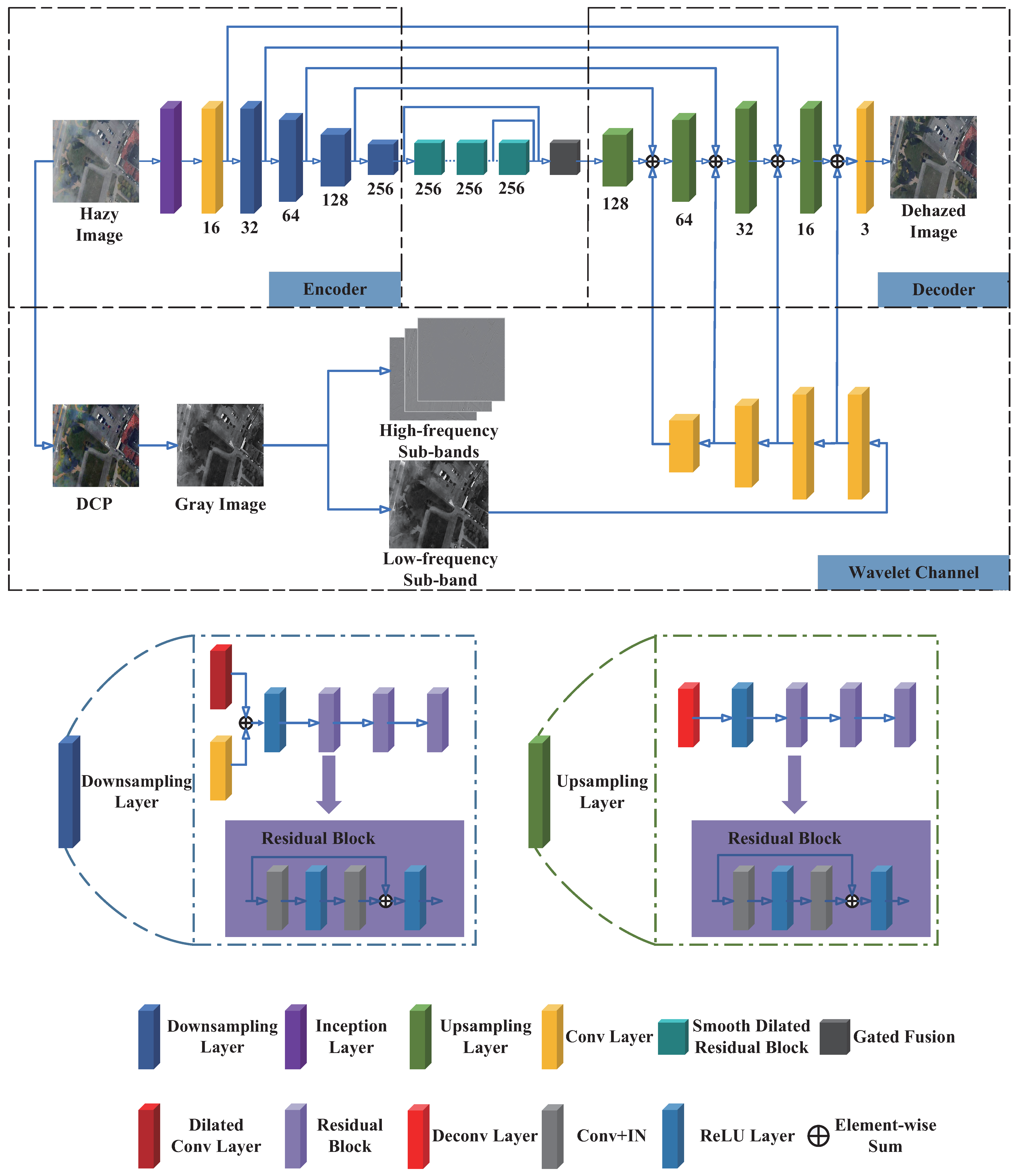
- Firstly, a single RS image dehazing method, which combines both wavelet transform and deep learning technology, is proposed. We employ the atmospheric scattering model and 2D stationary wavelet transform (SWT) to process a hazy image, and extract the low-frequency sub-band information of the processed image as the enhanced features to further strengthen the learning ability of the deep network for low-frequency smooth information in RS images.
- Secondly, our dehazing method is based on the encoder–decoder architecture. The inception structure in the encoder can increase the multi-scale information and learn the abundant image features for our network. As the hybrid convolution in the encoder combines standard convolution with dilated convolution, it expands the receptive field to better improve the ability of detecting the non-uniform haze in RS images. The decoder fusions the shallow feature information of the network through multiple residual blocks to recover the detailed information of the RS images.
- Thirdly, a special design in the aspect of loss function is made for the non-uniform dehazing task of RS images. As the scene structure edges of an RS image itself are usually weak, the structure pixels are weakened more seriously after dehazing. Therefore, on the basis of the L1 loss function, we employ the multi-scale structural similarity index (MS-SSIM) and Sobel edge detection as the loss function to make the dehazed image more natural and improve the edge of the dehazed RS images.
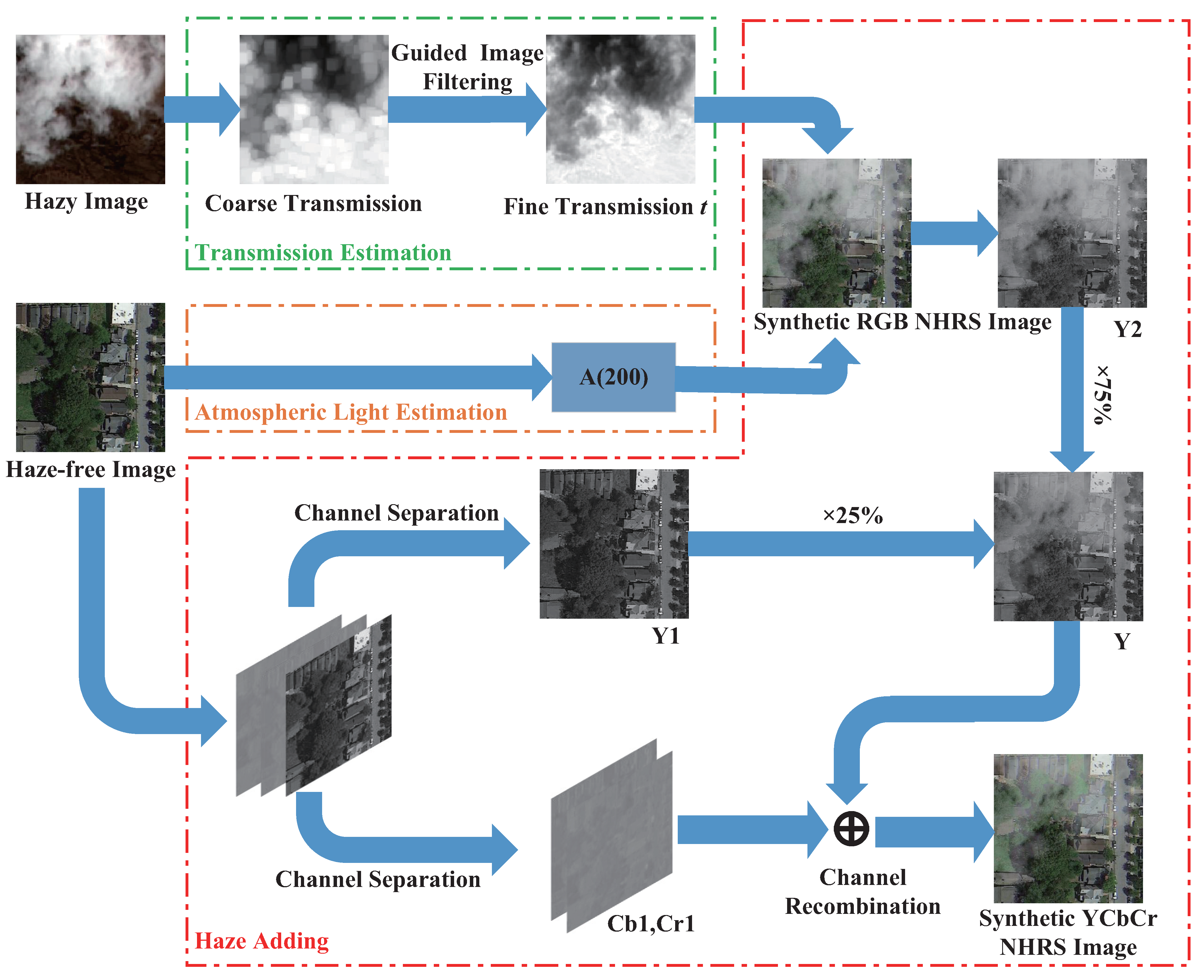
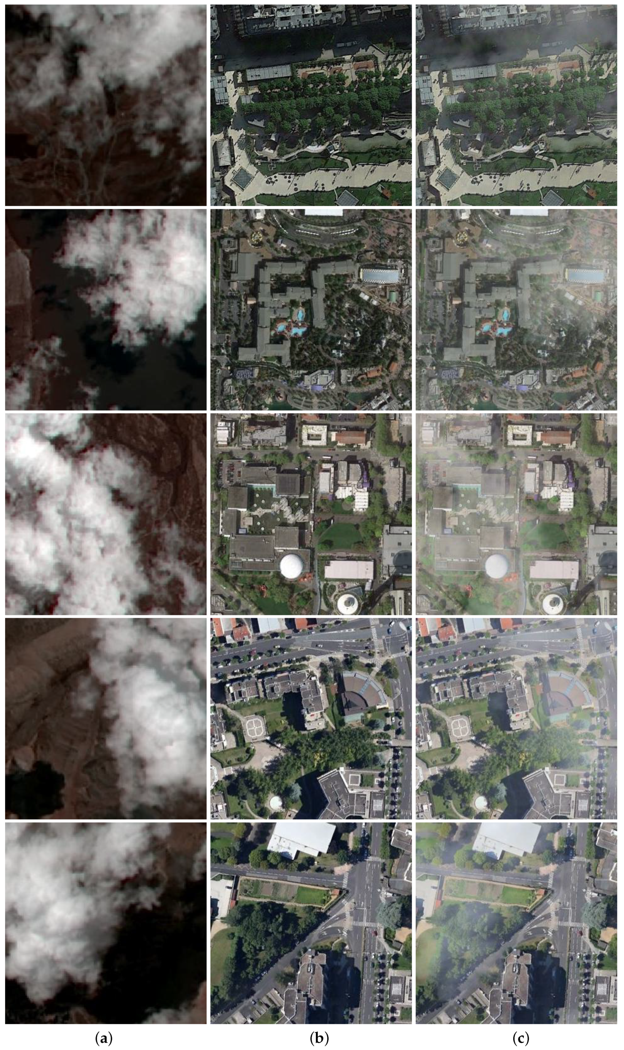
- Lastly, aiming at the problem that a deep learning network depends on the support of high-quality datasets, we propose a non-uniform haze-adding algorithm to establish a large-scale hazy RS image dataset. We employ the transmission of the real hazy image and the atmospheric scattering model in the RGB color space to obtain the RGB synthetic hazy image. The haze in a hazy image is mainly distributed on the Y channel component of the YCbCr color space. Based on this distribution characteristic of haze, the RGB synthetic hazy image and the haze-free image are jointly corrected to obtain the final synthetic NHRS image in the YCbCr color space.
2. Related Work
2.1. Traditional Dehazing Methods
2.2. Dehazing Methods Based on Deep Learning
3. Proposed Method
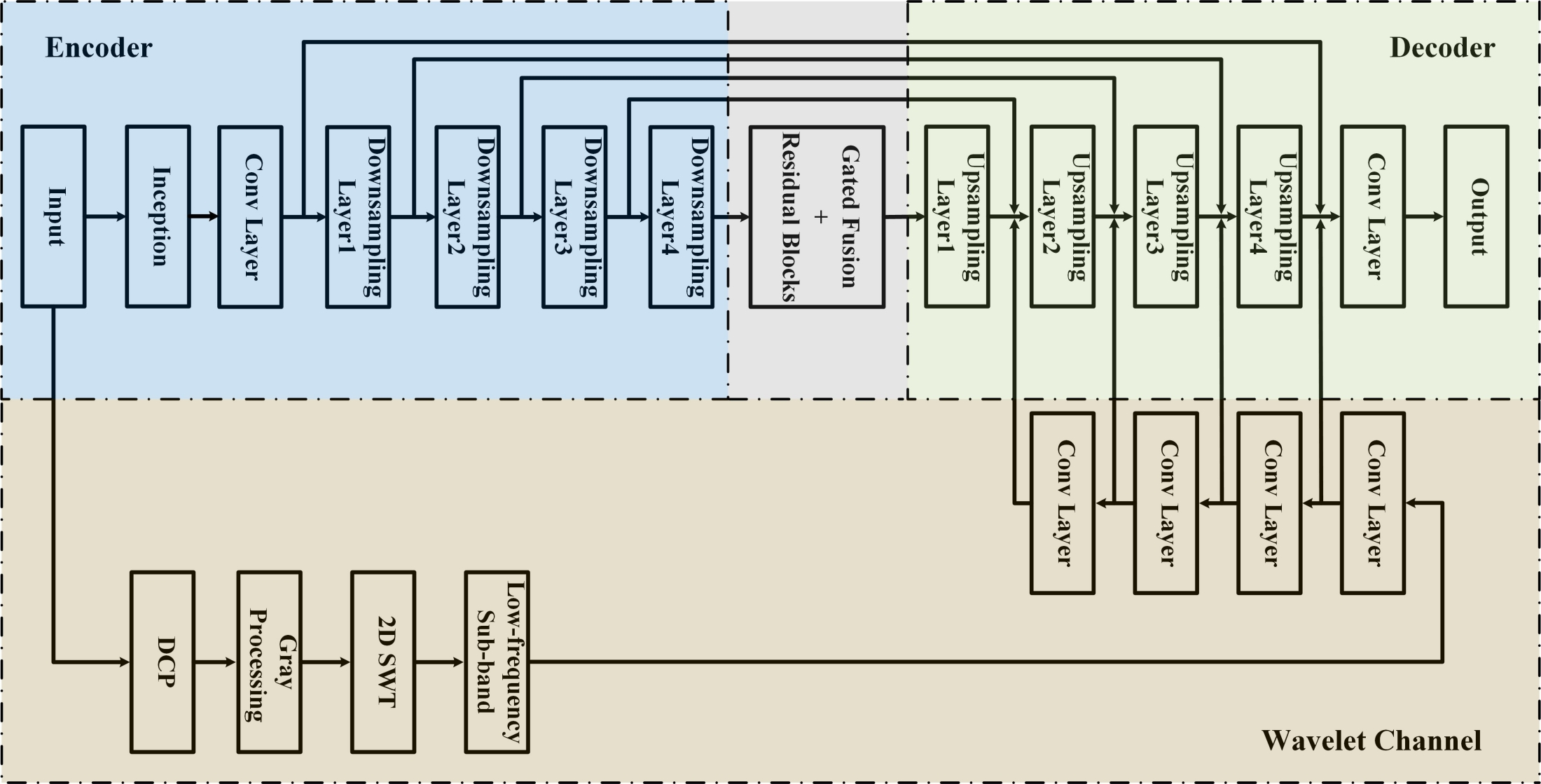
3.1. Network Architecture
3.2. Loss Function Design
3.3. Non-Uniform Haze Adding Algorithm
4. Experiment and Discussion
4.1. Experiment of Non-Uniform Haze-Adding Algorithm
4.1.1. Implementation Details
4.1.2. Dataset Establishment
4.2. Experiment of Proposed Dehazing Method
4.2.1. Training Details
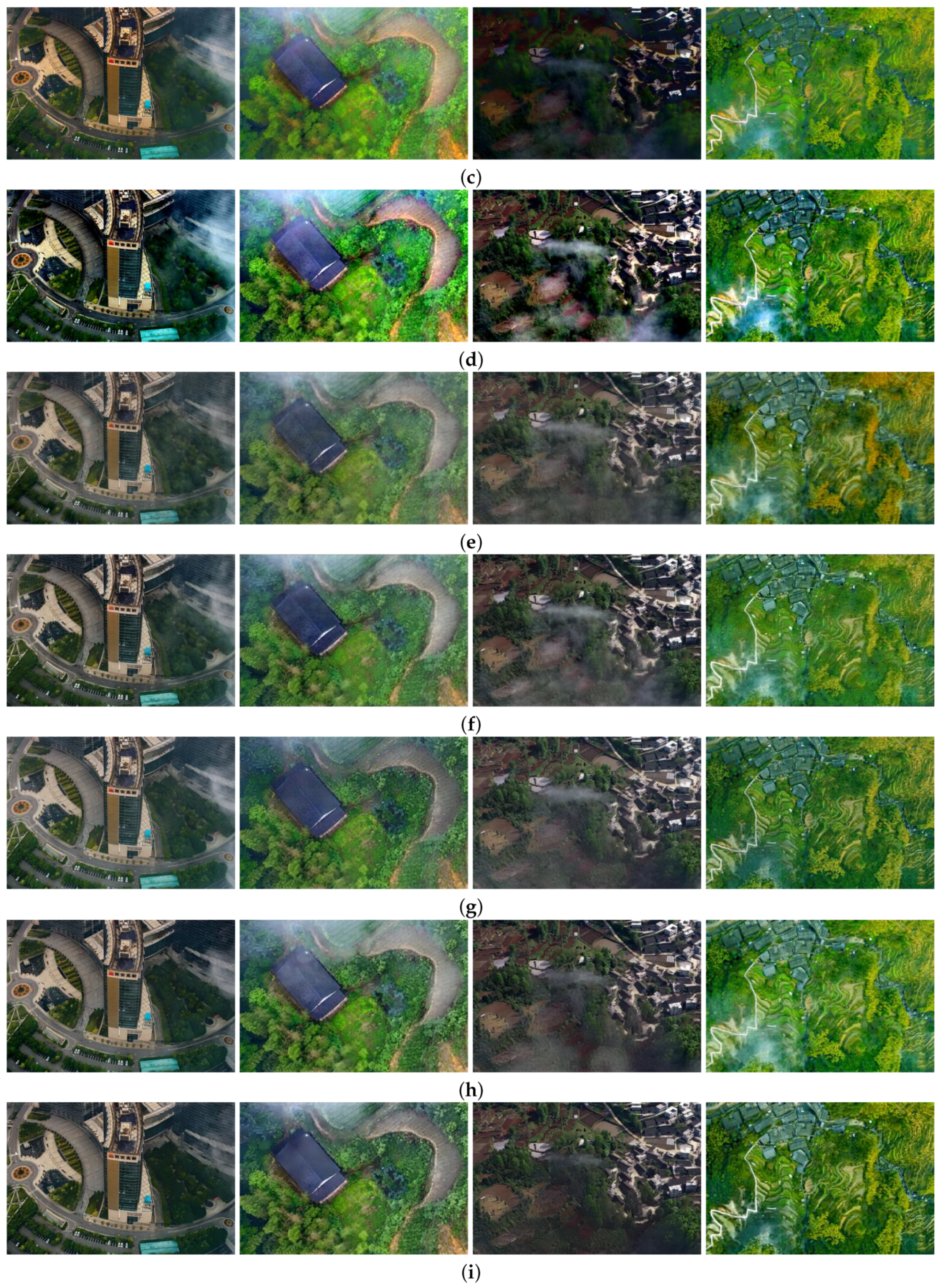
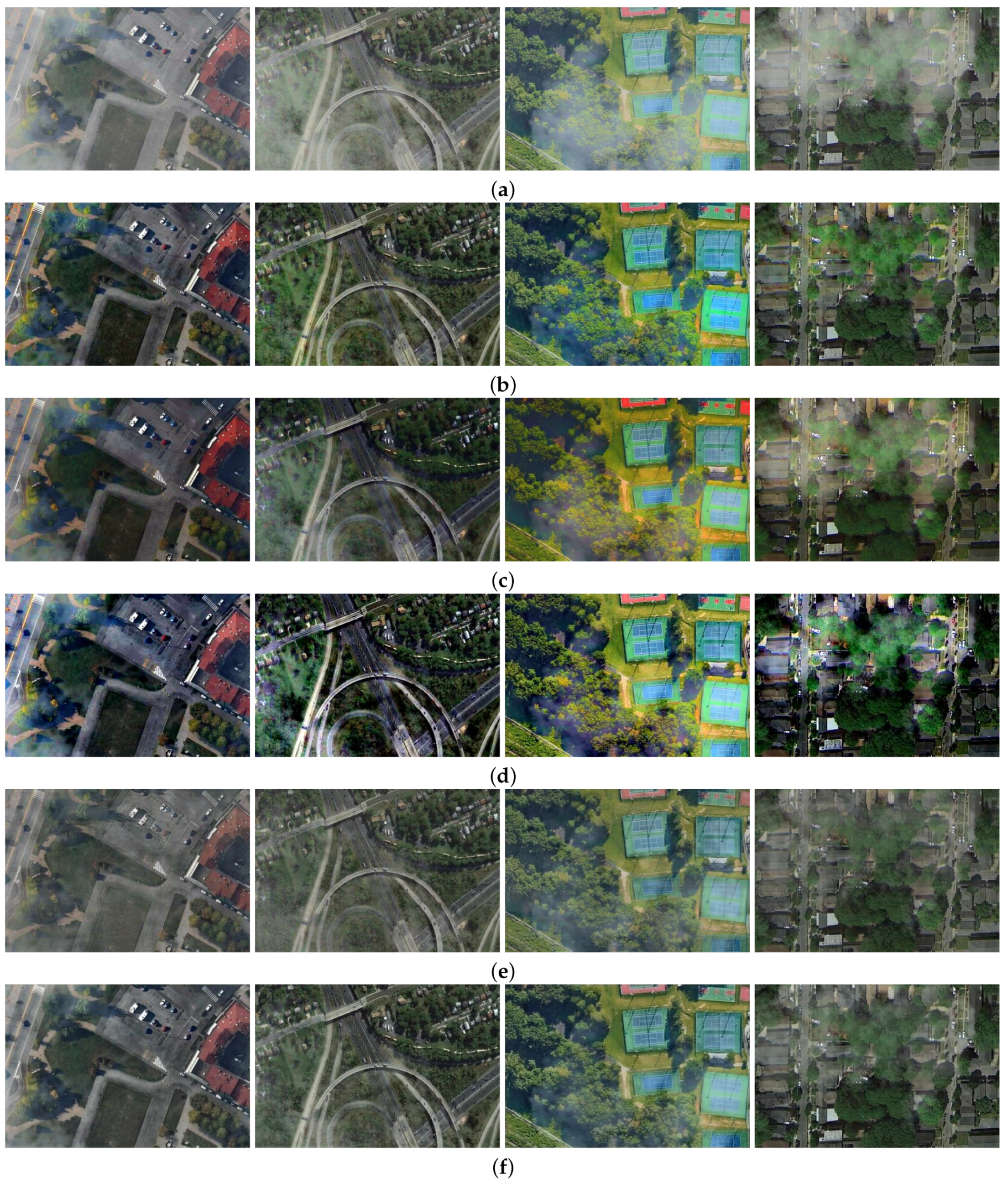
4.2.2. Result Evaluation
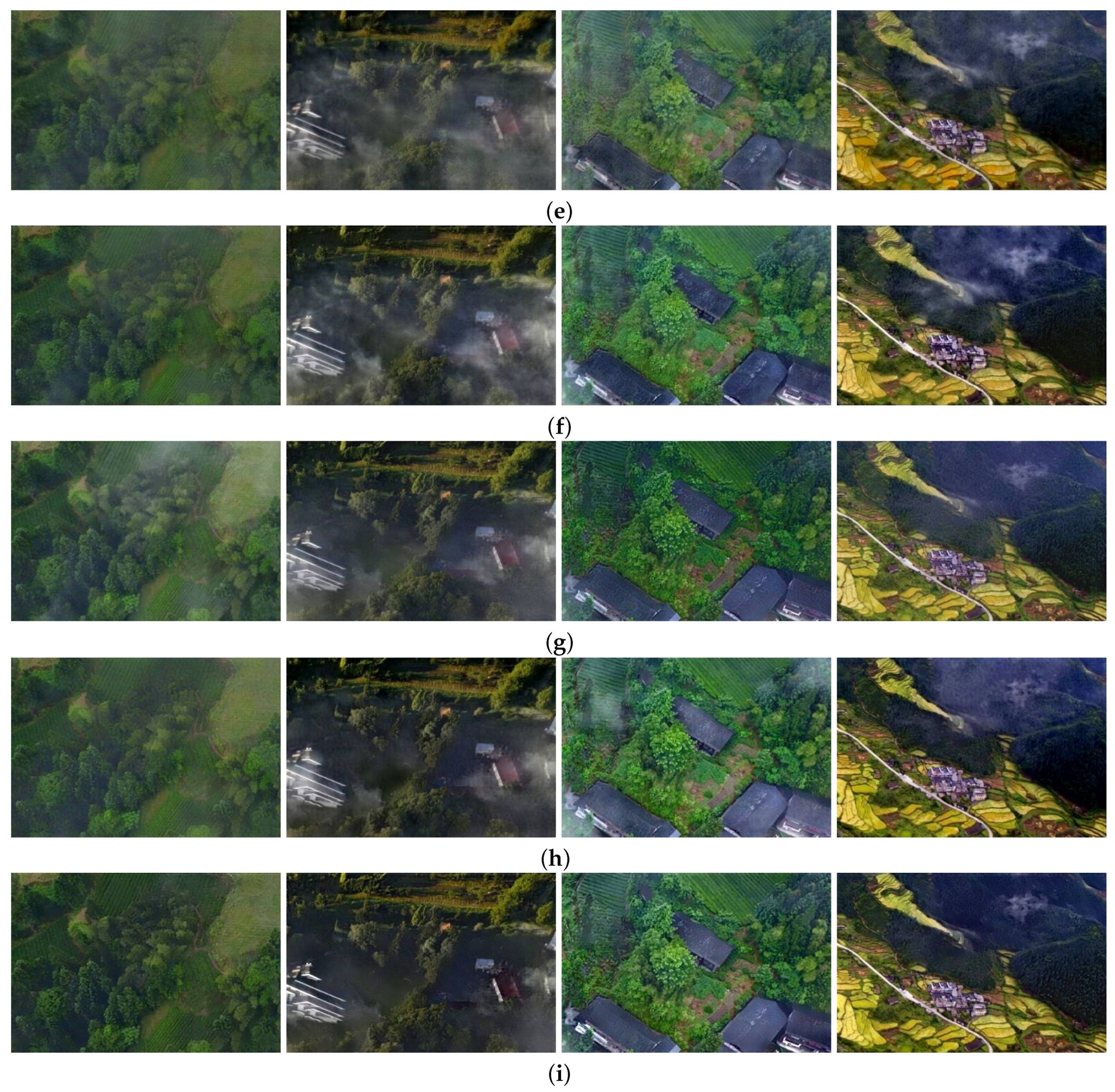
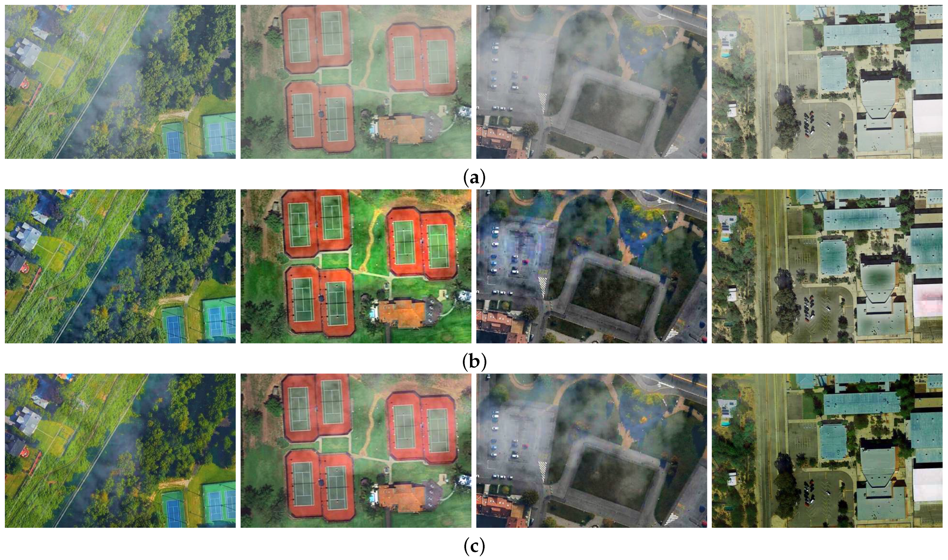
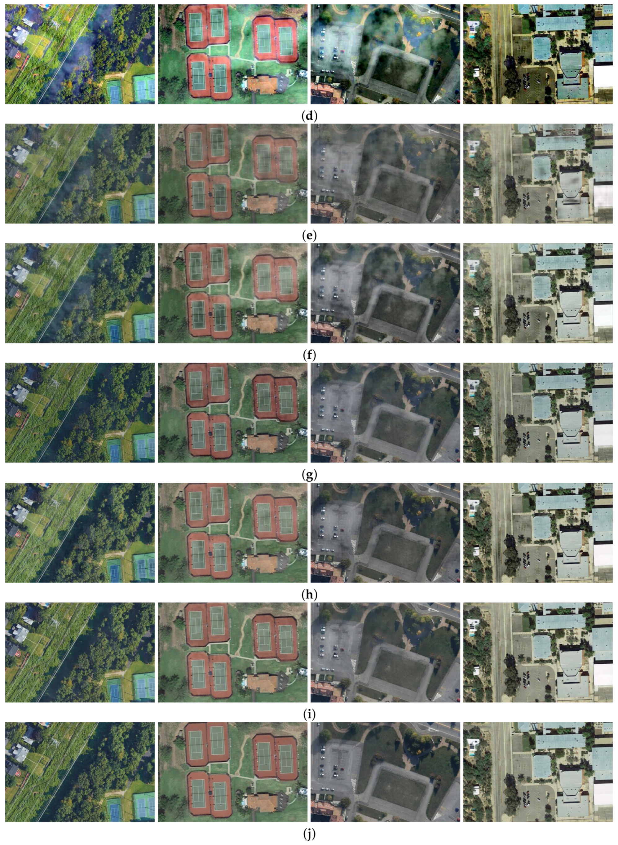
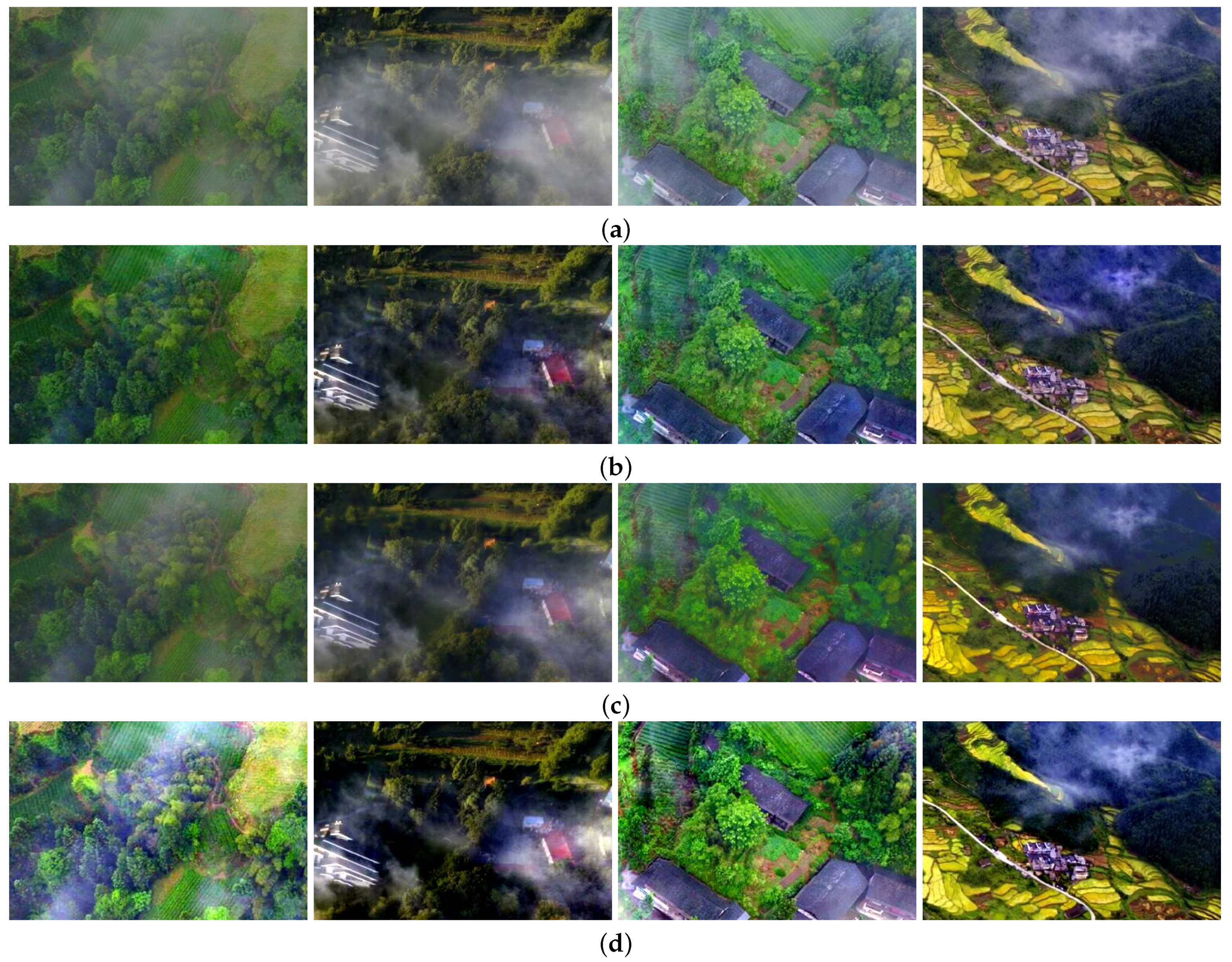
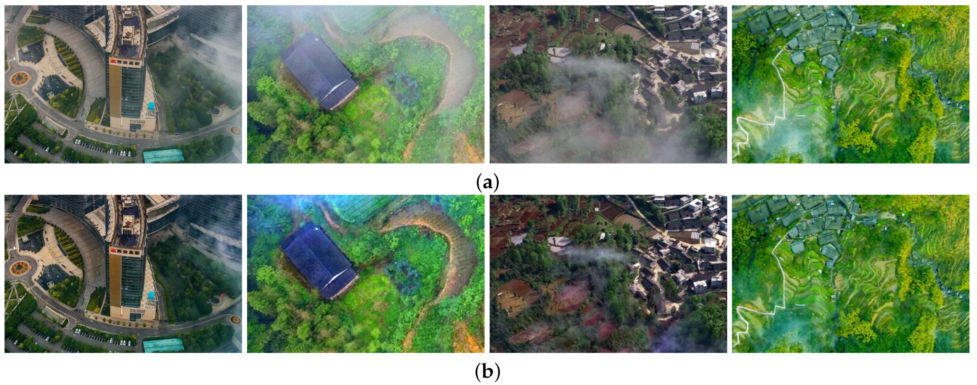
Qualitative Evaluation
Quantitative Evaluation
4.2.3. Discussion
5. Conclusions
Author Contributions
Funding
Data Availability Statement
Conflicts of Interest
Abbreviations
| RS | Remote sensing |
| NHRS | Non-uniform haze remote sensing |
| SWT | Stationary wavelet transform |
| PSNR | Peak signal-to-noise ratio |
| SSIM | Structural similarity |
| FSIM | Feature similarity |
References
- Wierzbicki, D.; Kedzierski, M.; Grochala, A. A Method for Dehazing Images Obtained from Low Altitudes during High-Pressure Fronts. Remote Sens. 2019, 12, 25. [Google Scholar] [CrossRef] [Green Version]
- Zhu, Z.; Luo, Y.; Wei, H.; Li, Y.; Qi, G.; Mazur, N.; Li, Y.; Li, P. Atmospheric Light Estimation Based Remote Sensing Image Dehazing. Remote Sens. 2021, 13, 2432. [Google Scholar] [CrossRef]
- Mccartney, E.J.; Hall, F.F. Optics of the Atmosphere: Scattering by Molecules and Particles. Phys. Today 1977, 30, 76–77. [Google Scholar] [CrossRef]
- Narasimhan, S.G.; Nayar, S.K. Chromatic Framework for Vision in Bad Weather. In Proceedings of the IEEE Conference on Computer Vision and Pattern Recognition—CVPR 2000, Hilton Head, SC, USA, 15 June 2000; pp. 598–605. [Google Scholar]
- Narasimhan, S.G.; Nayar, S.K. Vision and the atmosphere. Int. J. Comput. Vis. 2002, 48, 233–254. [Google Scholar] [CrossRef]
- He, K.; Sun, J.; Tang, X. Single Image Haze Removal Using Dark Channel Prior. IEEE Trans. Pattern Anal. Mach. Intell. 2011, 33, 2341–2353. [Google Scholar] [PubMed]
- Fattal, R. Single Image Dehazing. ACM Trans. Graph. 2008, 27, 1–9. [Google Scholar] [CrossRef]
- Berman, D.; Treibitz, T.; Avidan, S. Non-local Image Dehazing. In Proceedings of the IEEE Conference on Computer Vision and Pattern Recognition—CVPR 2016, Las Vegas, NV, USA, 27–30 June 2016; pp. 1674–1682. [Google Scholar]
- Zhu, Q.; Mai, J.; Shao, L. A Fast Single Image Haze Removal Algorithm Using Color Attenuation Prior. IEEE Trans. Image Process. 2015, 24, 3522–3533. [Google Scholar] [PubMed] [Green Version]
- Muhammad, K.; Mustaqeem; Ullah, A.; Imran, A.S.; Sajjad, M.; Kiran, M.S.; Sannino, G.; de Albuquerque, V.H.C. Human Action Recognition Using Attention Based LSTM Network with Dilated CNN Features. Future Gener. Comput. Syst. 2021, 125, 820–830. [Google Scholar] [CrossRef]
- Mustaqeem; Kwon, S. Optimal Feature Selection Based Speech Emotion Recognition Using Two-Stream Deep Convolutional Neural Network. Int. J. Intell. Syst. 2021, 36, 5116–5135. [Google Scholar] [CrossRef]
- Mei, K.; Jiang, A.; Li, J.; Wang, M. Progressive Feature Fusion Network for Realistic Image Dehazing. In Proceedings of the Asian Conference on Computer Vision—ACCV 2018, Perth, Australia, 2–6 December 2018; pp. 203–215. [Google Scholar]
- Yang, H.H.; Fu, Y. Wavelet U-Net and the Chromatic Adaptation Transform for Single Image Dehazing. In Proceedings of the IEEE International Conference on Image Processing—ICIP 2019, Taipei, Taiwan, 22–25 September 2019; pp. 2736–2740. [Google Scholar]
- Qu, Y.; Chen, Y.; Huang, J.; Xie, Y. Enhanced Pix2pix Dehazing Network. In Proceedings of the IEEE/CVF Conference on Computer Vision and Pattern Recognition—CVPR 2019, Long Beach, CA, USA, 15–20 June 2019; pp. 8152–8160. [Google Scholar]
- Li, Y.; Chen, X. A Coarse-to-Fine Two-stage Attentive Network for Haze Removal of Remote Sensing Images. IEEE Geosci. Remote Sens. 2020, 18, 1751–1755. [Google Scholar] [CrossRef]
- Szegedy, C.; Liu, W.; Jia, Y.; Sermanet, P.; Rabinovich, A. Going Deeper with Convolutions. In Proceedings of the IEEE Conference on Computer Vision and Pattern Recognition—CVPR 2015, Boston, MA, USA, 7–12 June 2015; pp. 1–9. [Google Scholar]
- Yu, F.; Koltun, V. Multi-scale Context Aggregation by Dilated Convolutions. In Proceedings of the International Conference on Learning Representations—ICLR 2016, San Juan, PR, USA, 2–4 May 2016; pp. 1–13. [Google Scholar]
- He, K.; Zhang, X.; Ren, S.; Sun, J. Deep Residual Learning for Image Recognition. In Proceedings of the IEEE Conference on Computer Vision and Pattern Recognition—CVPR 2016, Las Vegas, NV, USA, 27–30 June 2016; pp. 770–778. [Google Scholar]
- Ulyanov, D.; Vedaldi, A.; Lempitsky, V. Instance Normalization: The Missing Ingredient for Fast Stylization. arXiv 2016, arXiv:1607.08022. [Google Scholar]
- Chen, D.; He, M.; Fan, Q.; Liao, J.; Zhang, L.; Hou, D.; Yuan, L.; Hua, G. Gated Context Aggregation Network for Image Dehazing and Deraining. In Proceedings of the IEEE Winter Conference on Applications of Computer Vision—WACV 2019, Waikoloa, HI, USA, 7–11 January 2019; pp. 1375–1383. [Google Scholar]
- Wang, Z.; Ji, S. Smoothed Dilated Convolutions for Improved Dense Prediction. In Proceedings of the ACM SIGKDD International Conference on Knowledge Discovery and Data Mining—KDD 2018, London, UK, 19–23 August 2018; pp. 2486–2495. [Google Scholar]
- Deng, X.; Yang, R.; Xu, M.; Dragotti, P.L. Wavelet Domain Style Transfer for an Effective Perception-Distortion Tradeoff in Single Image Super-Resolution. In Proceedings of the IEEE/CVF International Conference on Computer Vision—ICCV 2019, Seoul, Korea, 27 October–2 November 2019; pp. 3076–3085. [Google Scholar]
- Zhou, W.; Bovik, A.C.; Sheikh, H.R.; Simoncelli, E.P. Image Quality Assessment: From Error Visibility to Structural Similarity. IEEE Trans. Image Process. 2004, 13, 600–612. [Google Scholar]
- Zhou, W.; Simoncelli, E.P.; Bovik, A.C. Multiscale Structural Similarity for Image Quality Assessment. In Proceedings of the Thrity-Seventh Asilomar Conference on Signals, Systems and Computers, Pacific Grove, CA, USA, 9–12 November 2003; pp. 1398–1402. [Google Scholar]
- Zhao, H.; Gallo, O.; Frosio, I.; Kautz, J. Loss Functions for Image Restoration with Neural Networks. IEEE Trans. Comput. Imaging 2016, 3, 47–57. [Google Scholar] [CrossRef]
- He, K.; Sun, J.; Tang, X. Guided image filtering. IEEE Trans. Pattern Anal. Mach. Intell. 2013, 35, 1397–1409. [Google Scholar] [CrossRef] [PubMed]
- Dudhane, A.; Murala, S. RYF-Net: Deep Fusion Network for Single Image Haze Removal. IEEE Trans. Image Process. 2019, 29, 628–640. [Google Scholar] [CrossRef] [PubMed]
- Xia, G.-S.; Hu, J.; Hu, F.; Shi, B.; Bai, X.; Zhong, Y.; Zhang, L.; Lu, X. AID: A Benchmark Data Set for Performance Evaluation of Aerial Scene Classification. IEEE Trans. Geosci. Remote Sens. 2017, 55, 3965–3981. [Google Scholar] [CrossRef] [Green Version]
- Qin, Z.; Ni, L.; Tong, Z.; Qian, W. Deep Learning Based Feature Selection for Remote Sensing Scene Classification. IEEE Geosci. Remote Sens. 2015, 12, 2321–2325. [Google Scholar]
- BH-Pools/Watertanks Datasets. Available online: http://patreo.dcc.ufmg.br/2020/07/29/bh-pools-watertanks-datasets/ (accessed on 30 August 2021).
- Geospatial Data Cloud. Available online: http://www.gscloud.cn (accessed on 30 August 2021).
- Berman, D.; Treibitz, T.; Avidan, S. Air-light Estimation Using Haze-lines. In Proceedings of the IEEE International Conference on Computational Photography—ICCP 2017, Stanford, CA, USA, 12–14 May 2017; pp. 1–9. [Google Scholar]
- Zhang, L.; Zhang, L.; Mou, X.; Zhang, D. FSIM: A Feature Similarity Index for Image Quality Assessment. IEEE Trans. Image Process. 2011, 20, 2378–2386. [Google Scholar] [CrossRef] [PubMed] [Green Version]


| Layer | Local Structure | Output Size | Output Channel |
|---|---|---|---|
| Input | 3 | ||
| Inception | (Conv, (Conv | 3 | |
| Convolution | Conv | 16 | |
| ( Conv, s = 2, d = 1), ( Conv, s = 2, d = 2) | 32 | ||
| Downsampling Layer1 | ReLU | 32 | |
| Conv, IN, ReLU | 32 | ||
| ( Conv, s = 2, d = 1), ( Conv, s = 2, d = 2) | 64 | ||
| Downsampling Layer2 | ReLU | 64 | |
| Conv, IN, ReLU | 64 | ||
| ( Conv, s = 2, d = 1), ( Conv, s = 2, d = 2) | 128 | ||
| Downsampling Layer3 | ReLU | 128 | |
| Conv, IN, ReLU | 128 | ||
| ( Conv, s = 2, d = 1), ( Conv, s = 2, d = 2) | 256 | ||
| Downsampling Layer4 | ReLU | 256 | |
| Conv, IN, ReLU | 256 |
| Layer | Local Structure | Output Size | Output Channel |
|---|---|---|---|
| Deconv, s = 2 | 128 | ||
| Upsampling Layer1 | ReLU | 128 | |
| Deconv, IN, ReLU | 128 | ||
| Deconv, s = 2 | 64 | ||
| Upsampling Layer2 | ReLU | 64 | |
| Deconv, IN, ReLU | 64 | ||
| Deconv, s = 2 | 32 | ||
| Upsampling Layer3 | ReLU | 32 | |
| Deconv, IN, ReLU | 32 | ||
| Deconv, s = 2 | 16 | ||
| Upsampling Layer4 | ReLU | 16 | |
| Deconv, IN, ReLU | 16 | ||
| Convolution | Conv | 3 | |
| Dehazed output | 3 |
| Image | DCP | CAP | NLD | PFF-Net | W-U-Net | EPDN | FCTF-Net | Ours |
|---|---|---|---|---|---|---|---|---|
| Figure 4 1st column | 18.1757 | 16.8021 | 16.0314 | 22.1598 | 20.6270 | 25.1673 | 26.6991 | 26.9116 |
| Figure 4 2nd column | 23.0893 | 18.9500 | 16.8124 | 21.4356 | 21.7374 | 23.7852 | 27.1162 | 28.0056 |
| Figure 4 3rd column | 20.6492 | 17.9509 | 18.6025 | 21.2522 | 21.9921 | 23.7839 | 26.3346 | 28.1458 |
| Figure 4 4th column | 20.6405 | 16.2992 | 16.1343 | 19.4756 | 19.7069 | 25.5164 | 27.9014 | 28.6765 |
| Figure 5 1st column | 22.0578 | 19.9599 | 17.0074 | 22.5066 | 23.3277 | 23.6046 | 24.4548 | 27.4342 |
| Figure 5 2nd column | 17.7801 | 19.9324 | 16.7586 | 23.2878 | 22.2942 | 22.7151 | 27.2257 | 30.3904 |
| Figure 5 3rd column | 18.4220 | 17.4235 | 14.4382 | 21.3188 | 20.9592 | 27.1209 | 25.0667 | 28.2225 |
| Figure 5 4th column | 16.9078 | 13.5731 | 14.8070 | 21.7622 | 22.5752 | 23.5890 | 25.3069 | 28.4855 |
| Image | DCP | CAP | NLD | PFF-Net | W-U-Net | EPDN | FCTF-Net | Ours |
|---|---|---|---|---|---|---|---|---|
| Figure 4 1st column | 0.7791 | 0.7836 | 0.6383 | 0.8516 | 0.8706 | 0.9163 | 0.9229 | 0.9261 |
| Figure 4 2nd column | 0.8519 | 0.7744 | 0.6459 | 0.8315 | 0.8363 | 0.8743 | 0.8949 | 0.8991 |
| Figure 4 3rd column | 0.8570 | 0.7286 | 0.8036 | 0.8603 | 0.8874 | 0.9325 | 0.9415 | 0.9443 |
| Figure 4 4th column | 0.8231 | 0.7204 | 0.6052 | 0.7797 | 0.8074 | 0.8718 | 0.8984 | 0.9001 |
| Figure 5 1st column | 0.8646 | 0.8203 | 0.8051 | 0.8548 | 0.8797 | 0.9127 | 0.9188 | 0.9285 |
| Figure 5 2nd column | 0.7258 | 0.8717 | 0.7364 | 0.9072 | 0.9261 | 0.9346 | 0.9539 | 0.9617 |
| Figure 5 3rd column | 0.7220 | 0.8033 | 0.5719 | 0.8350 | 0.8550 | 0.9006 | 0.9014 | 0.9153 |
| Figure 5 4th column | 0.8431 | 0.6970 | 0.6738 | 0.8860 | 0.8900 | 0.9264 | 0.9306 | 0.9419 |
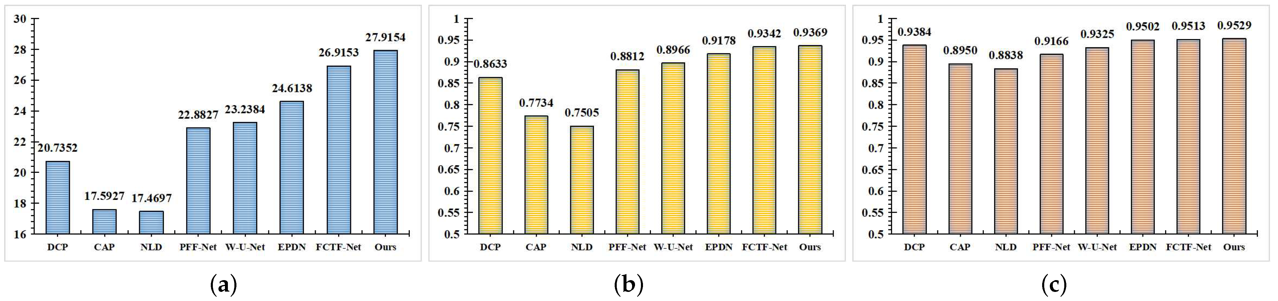
| Metrics | DCP | CAP | NLD | PFF-Net | W-U-Net | EPDN | FCTF-Net | Ours |
|---|---|---|---|---|---|---|---|---|
| PSNR | 20.7352 | 17.5927 | 17.4697 | 22.8827 | 23.2384 | 24.6138 | 26.9153 | 27.9154 |
| SSIM | 0.8633 | 0.7734 | 0.7505 | 0.8812 | 0.8966 | 0.9178 | 0.9342 | 0.9369 |
| FSIM | 0.9384 | 0.8950 | 0.8838 | 0.9166 | 0.9325 | 0.9502 | 0.9513 | 0.9529 |
Publisher’s Note: MDPI stays neutral with regard to jurisdictional claims in published maps and institutional affiliations. |
© 2021 by the authors. Licensee MDPI, Basel, Switzerland. This article is an open access article distributed under the terms and conditions of the Creative Commons Attribution (CC BY) license (https://creativecommons.org/licenses/by/4.0/).
Share and Cite
Jiang, B.; Chen, G.; Wang, J.; Ma, H.; Wang, L.; Wang, Y.; Chen, X. Deep Dehazing Network for Remote Sensing Image with Non-Uniform Haze. Remote Sens. 2021, 13, 4443. https://doi.org/10.3390/rs13214443
Jiang B, Chen G, Wang J, Ma H, Wang L, Wang Y, Chen X. Deep Dehazing Network for Remote Sensing Image with Non-Uniform Haze. Remote Sensing. 2021; 13(21):4443. https://doi.org/10.3390/rs13214443
Chicago/Turabian StyleJiang, Bo, Guanting Chen, Jinshuai Wang, Hang Ma, Lin Wang, Yuxuan Wang, and Xiaoxuan Chen. 2021. "Deep Dehazing Network for Remote Sensing Image with Non-Uniform Haze" Remote Sensing 13, no. 21: 4443. https://doi.org/10.3390/rs13214443
APA StyleJiang, B., Chen, G., Wang, J., Ma, H., Wang, L., Wang, Y., & Chen, X. (2021). Deep Dehazing Network for Remote Sensing Image with Non-Uniform Haze. Remote Sensing, 13(21), 4443. https://doi.org/10.3390/rs13214443