Abstract
We present a proof of concept of wind turbine wake identification and characterization using a region-based convolutional neural network (CNN) applied to lidar arc scan images taken at a wind farm in complex terrain. We show that the CNN successfully identifies and characterizes wakes in scans with varying resolutions and geometries, and can capture wake characteristics in spatially heterogeneous fields resulting from data quality control procedures and complex background flow fields. The geometry, spatial extent and locations of wakes and wake fragments exhibit close accord with results from visual inspection. The model exhibits a 95% success rate in identifying wakes when they are present in scans and characterizing their shape. To test model robustness to varying image quality, we reduced the scan density to half the original resolution through down-sampling range gates. This causes a reduction in skill, yet 92% of wakes are still successfully identified. When grouping scans by meteorological conditions and utilizing the CNN for wake characterization under full and half resolution, wake characteristics are consistent with a priori expectations for wake behavior in different inflow and stability conditions.
1. Introduction
Wind turbine wakes are turbulent low-velocity flow structures that interact with downstream turbines, decreasing the inflow speed and turbine performance while increasing the blade fatigue [1,2,3,4]. Knowledge of wake trajectory, geometry and orientation is pertinent to power production and fatigue analyses. However, there is uncertainty in both identifying wakes and defining wake metrics. Wake identification and characterization methods have been introduced to quantify the behavior of wakes and applied to simulation outputs and measurements over flat terrain [5,6]. Even under these relatively simple datasets, methodologies still exhibit difficulties in distinguishing the wind turbine wake from local turbulent flows, particularly at distances far behind the rotor [7]. Further, variations in the local orography in and around wind farms enhance turbulence and flow complexity, thus rendering wind turbine wake identification, characterization and tracking more difficult [8].
Methods to identify wakes from remote sensing (e.g., lidar) data commonly depend on the availability of information, such as the wind turbine rotor diameter, free-stream wind speed, atmospheric stability, scan resolution and geometry [9,10]. Many wake detection methods approximate the location and area of the wake’s center through fitting Gaussian curves to line-of-sight (LOS) velocity deficits, implementing contour-based methods utilizing momentum flux or a velocity deficit and using the turbulence profile method [5,11,12].
Wake detection methods in complex terrain have been implemented with varying degrees of success, and focus on identifying the wake center for a single wind turbine [13,14]. An automated wake detection method was proposed to identify the wake centerline from lidar measurements in complex terrain by using knowledge of the turbine’s location and flow-field anomalies [8]. A second dynamic model for wake identification and characterization in complex terrain using lidar measurements identified the wake centerline from a single wind turbine using a wake velocity deficit and dynamic wake meandering models [15].
Although identifying the wake centerline of a single wind turbine is pertinent to understanding the propagation of wakes downstream in complex terrain, there remains a need for automated (scan campaigns often result in thousands of scans that require processing) holistic wake identification and characterization methods that can be implemented independently of varying experimental parameters and applied to flow fields with any number of wind turbine wakes. Furthermore, a method that can track the entirety of the wake (as well as partial wakes), including its exact shape as it forms and dissipates, is necessary to progress toward an enhanced understanding of wind turbine wake dynamics in complex terrain. Previously proposed methods exhibit a relatively high fidelity for identifying well-defined single wakes, but lack skill in identifying and characterizing asymmetric (skewed) or partial wakes resulting from turbulence or intentional wake steering. As many wake identification methods employ assumptions about the wake shape (e.g., Gaussian distributions), behavior of the wake center (e.g., maximum velocity deficit method) and definition of wake edges (e.g., assuming the wake diameter is equal to the rotor diameter), a model that can operate independently of these assumptions is pertinent to a broader range of datasets and applications.
Machine-learning techniques are adept at modeling, learning and predicting patterns from data [16,17], and are being used for applications such as wind plant power output prediction, wind resource prediction and even wake modeling [18,19,20,21,22]. Neural networks are machine-learning models that iteratively learn and assign meaning to patterns in input data through a series of neurons (also known as nodes) arranged in layers [23,24,25]. They have been demonstrated to be effective in interpreting multiple types of inputs, including sound, images and raw numerical data [26,27,28], and provide an ideal tool for understanding and interpreting the complexities and patterns in wind turbine wake flows in complex terrain [29]. Neural networks have the potential to address multiple common issues in wind turbine wake characterization and identification in complex terrain: simultaneously identifying the exact wake structures and characteristics of multiple wind turbine wakes; distinguishing flow-field turbulent structures generated by wakes from those embedded in the background atmospheric flow; identifying turbulent wake dissipation; and even locating wakes in lidar data that wind up incomplete or limited in spatial resolution after filtering for a low signal-to-noise (SNR) or carrier-to-noise ratio (CNR).
Although there are many forms of neural networks available, this work focuses on implementing a convolutional neural network (CNN). CNNs are commonly used for image processing and object detection or instance segmentation [30,31]. A CNN can analyze input images and identify objects based on their type, quantity, location and size. CNNs have been trained on datasets of varying complexity and have accurately performed complex tasks, such as detecting ships from synthetic aperture radar scans and identifying fish species from images [32,33]. Although CNN models continue to grow in complexity and capability, recent developments in these models have improved their computational time [34]. Traditional CNN models struggled with or were unable to detect multiple instances of objects within an image until the development of a region-based CNN (R-CNN) [35]. From R-CNN, Mask R-CNN was developed to output image segmentation masks for multiple instances of objects within an image [36]. In this context, a mask is a binary pixel matrix representing the exact location and size of detected objects. Mask R-CNN has been shown to identify and characterize objects in remote-sensing data robustly and successfully, such as identifying buildings from satellite imagery and mapping topographic features captured with lidar data [37,38]. As a result of its computational efficiency and accuracy in object segmentation and classification, the Mask R-CNN is a robust option for identifying and characterizing wind turbine wakes in complex terrain.
The objective of this research is to implement and evaluate a Mask R-CNN for wake identification and characterization using lidar data collected in complex terrain. The primary objectives of this proof of concept are to quantify the skill with which the CNN can: (i) identify multiple wind turbine wakes simultaneously from a variety of scan orientations (flow field quadrant, elevation angle, range coverage and resolution, time of day), (ii) characterize wake shapes as the wakes form and dissipate in the flow field and (iii) identify wakes even if they are obscured by missing data points. All objectives are evaluated over a range of wind turbine layout geometries (single and multiple rows of turbines and/or individual turbines).
2. Materials and Methods
2.1. Measurement Campaign
The lidar data used for this work were collected at a wind farm in the Pacific Northwest during a six-month period from July 2018–December 2018 (inclusive), using a WINDCUBE 100s Doppler wind lidar from Leosphere (described in further detail in [39]). For a majority of the scans in the campaign, the lidar returned line-of-sight velocities at a range gate resolution of 50 m. Scans were collected at varying azimuth and elevation angles relative to the lidar (elevation angles spanning from approximately 0° to upwards of 60°). The wind farm contains wind turbines that have hub heights (HH) of 80 m and rotor diameters (D) of 90 m. The campaign produced around 13,000 scans collectively. The analysis here focuses on arc scans only when wakes were present.
The campaign focused on flow into and downwind of a set of nine wind turbines: three to the northwest of the lidar and six to the southwest (Figure 1a). Often, wakes from two rows of turbines to the southeast and southwest of the lidar are visible, giving the opportunity to evaluate the algorithm’s performance when multiple wakes and rows of wakes are present (Figure 1a).
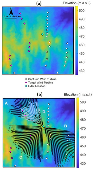
Figure 1.
(a) Elevation map (colored contours show elevation) of scanning site with target turbines (pink) and all turbines captured (white). The lidar location is indicated by the cyan diamond. (b) Regions A, B, C and D (shown as dotted areas) are utilized to illustrate model performance in the results section. Note that Region D (lavender) is within Region A. Regions do not represent coverage of a single scan; rather, scans as displayed by each region are unique and collected at different times in July and September.
2.2. Lidar Scan Filtering, Classification and Quality Control
Hub-height wind speed and direction during the scans are estimated as the mean values from supervisory control and data acquisition (SCADA) measurements obtained with cup anemometers and wind vanes on the nacelles of three of the target wind turbines. The data are conditionally sampled to select periods when the lidar was operating in arc scan configuration, and the HH wind speed (U) and direction are consistent with wake generation and propagation from the wind turbines deployed:
A total of 3307 scans meet these criteria for wind direction, wind speed and arc scan classification (around 25% of scans). Much of the rotational speed for the arc scans was kept constant at 1°/s, meaning that the lidar rotated one degree per second while moving through its scanning arc. Further, angular resolutions were kept consistent at 1°.
Radial velocity values are then filtered to remove values with high measurement uncertainty and include only those where:
2.3. Scan Preparation for CNN Training and Testing
Horizontal wind components in a cartesian coordinate system (, ) for each scan are estimated from radial (i.e., line-of-sight) velocity measurements ( under the assumptions that the projection of the vertical wind speed is zero and the flow field is relatively homogeneous. This method to reconstruct the horizontal wind field has been widely used and validated in previous studies, including a study that evaluated wind turbine wake characteristics from lidar scans taken near an escarpment [6,40]. and are related to the radial velocity measurements () through elevation and azimuth () angles as follows:
Through least squares linear regression, values for and per scan and estimated wind direction α (note that this is not local wind direction, as a single wind direction value is obtained per scan) are derived [40]:
The horizontal wind speed at each scanned volume relative to the lidar coordinate system is given by:
Reconstruction of the scan flow field enhances the visibility of the wind turbine wakes (Figure 2a,b) that are further clarified by normalizing the entire flow field by the mean wind speed. A high-contrast colormap is then applied to the normalized flow field velocity to isolate all regions of low-velocity flow and to visually homogenize all other freestream velocities (Figure 2c).

Figure 2.
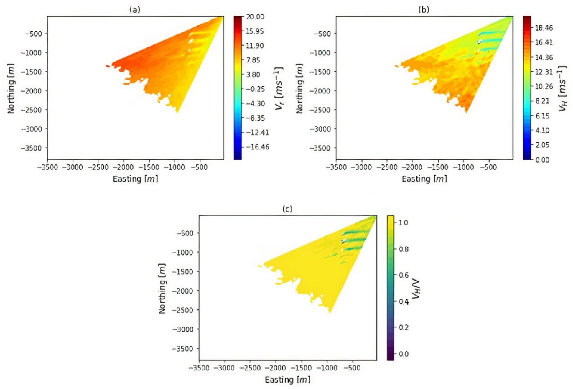
Example visualization of the flow field reconstruction: (a) radial wind speed (i.e., LOS velocity) as measured by the lidar; (b) transformation to estimated horizontal wind speed; and (c) normalization through estimated bulk wind speed per scan. Northing and easting distances in (a–c) are calculated relative to the lidar position. Data are for 3 November 2018, 04:58 UTC, elevation angle = 3°, azimuth angle , azimuthal resolution 1°, range gate 50 m, 40 s scan time.
To train the CNN on the simplest representation of the data, scan images are input into the model as an array of RGB pixels (Figure 3). Due to the fact that each scan image is cropped at known maximum and minimum northing and easting values, a conversion between pixels and meters (relative to the lidar) is possible. Thus, the model returns masks (a binary pixel array) for identified wakes, and the shape and relative location (in meters) of the wakes in the flow field are known. In this work, scan image dimensions are kept constant at 217 (width, south-north) by 334 (length, east-west) pixels. Any velocity values removed from the scan due to CNR filtering (e.g., hard-target returns at the wind turbine locations) are represented in black and remain in the scan images. Leaving filtered regions in the scans preserves the original scan geometry and ensures that a wide variety of scan geometries and aspect ratios are introduced to the model during training.

Figure 3.
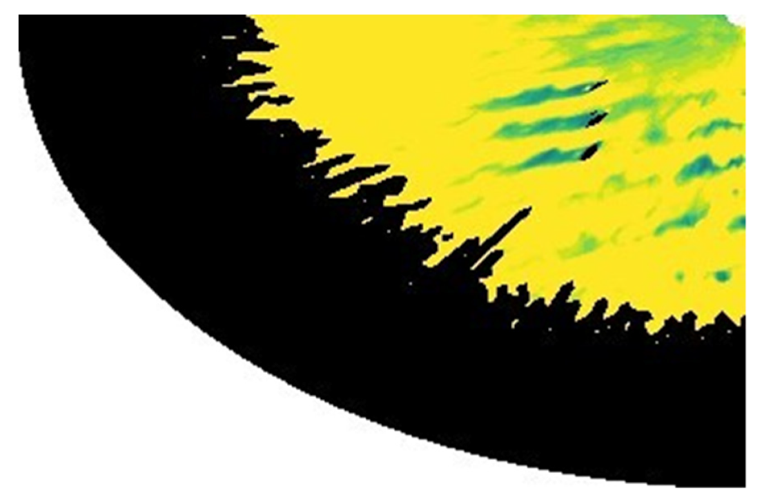
Example of training scan collected under easterly flow. Missing velocity measurements as assessed by carrier-to-noise ratio (CNR) values are shown in black. Data captured on 30 July 2018, 04:38 UTC, elevation angle = 1.5°, azimuth angle , azimuthal resolution 1°, range gate 50 m, 120 s scan time. Scan image dimensions are 217 (width) by 334 (length) pixels.
2.4. The Proof-of-Concept Dataset: Methodology
Out of the 3307 available arc scans, we selected a subset of 354 to design a proof-of-concept dataset. The sub-selection was based on the following objective criteria:
- Wakes cannot mix with each other, i.e., all wakes must be distinct;
- Wakes mut be distinct from local flow features (i.e., edges must be detectable amid local turbulent structures).
Scans were subject to both criteria through visual inspection. The majority of rejected scans exhibited discernible wakes, but displayed wake mixing and thus violated criterion (1). Cases in which CNR filtering obscured the wake shape were included in the dataset to evaluate the model’s efficacy in identifying wakes in regions of low-quality measurements. The 354-scan dataset was split into three subsets: two-thirds of the scans were selected for the training subset, whereas the remaining one-third was split evenly between the validation subset and testing subset. Although 354 scans represent approximately 10% of the original arc scan subset, there are over 1000 instances of wakes within these scans. Further, many arc scans were disqualified from inclusion in the proof-of-concept dataset, since they were taken at high elevation angles to survey the atmospheric conditions during scan collection time, and thus did not exhibit wakes. Wakes are visible in all scans in the proof-of-concept dataset; due to the methodology of Mask R-CNN (proposes regions of interest within the images; if there are no regions of interest, Mask R-CNN will identify no objects), there is no need to train the model on scan images without wakes. The model was trained using the training subset, and the validation subset was utilized to ensure the model is not overfit or underfit during training. The model was then evaluated using the independent testing subset. Subset scans encompassed a wide variety of scan geometries and parameters (Figure 4).
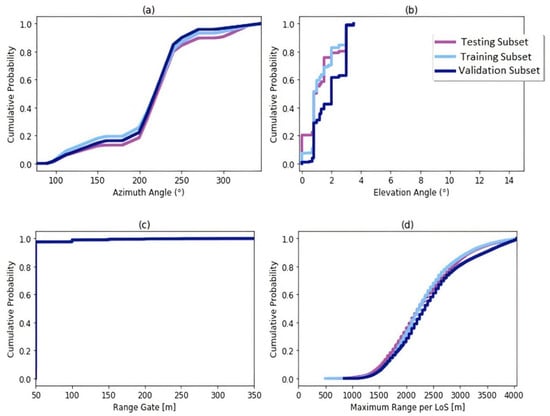
Figure 4.
Cumulative density functions for scan parameters: (a) azimuth and (b) elevation angles, (c) range gate and (d) maximum range per LOS for all scans included in each subset of the selected scans (training, testing, validation).
The model evaluation metrics in Section 3 rely on the following objective definition of wakes and wake fragments (dissipated wakes) (Figure 5). Wakes are defined as the first instance of low velocity flow emanating from a known turbine location. Wake fragments are defined as any background low-speed turbulent structures parallel to known wakes in the scan or collinear with wakes emanating from known turbine locations.

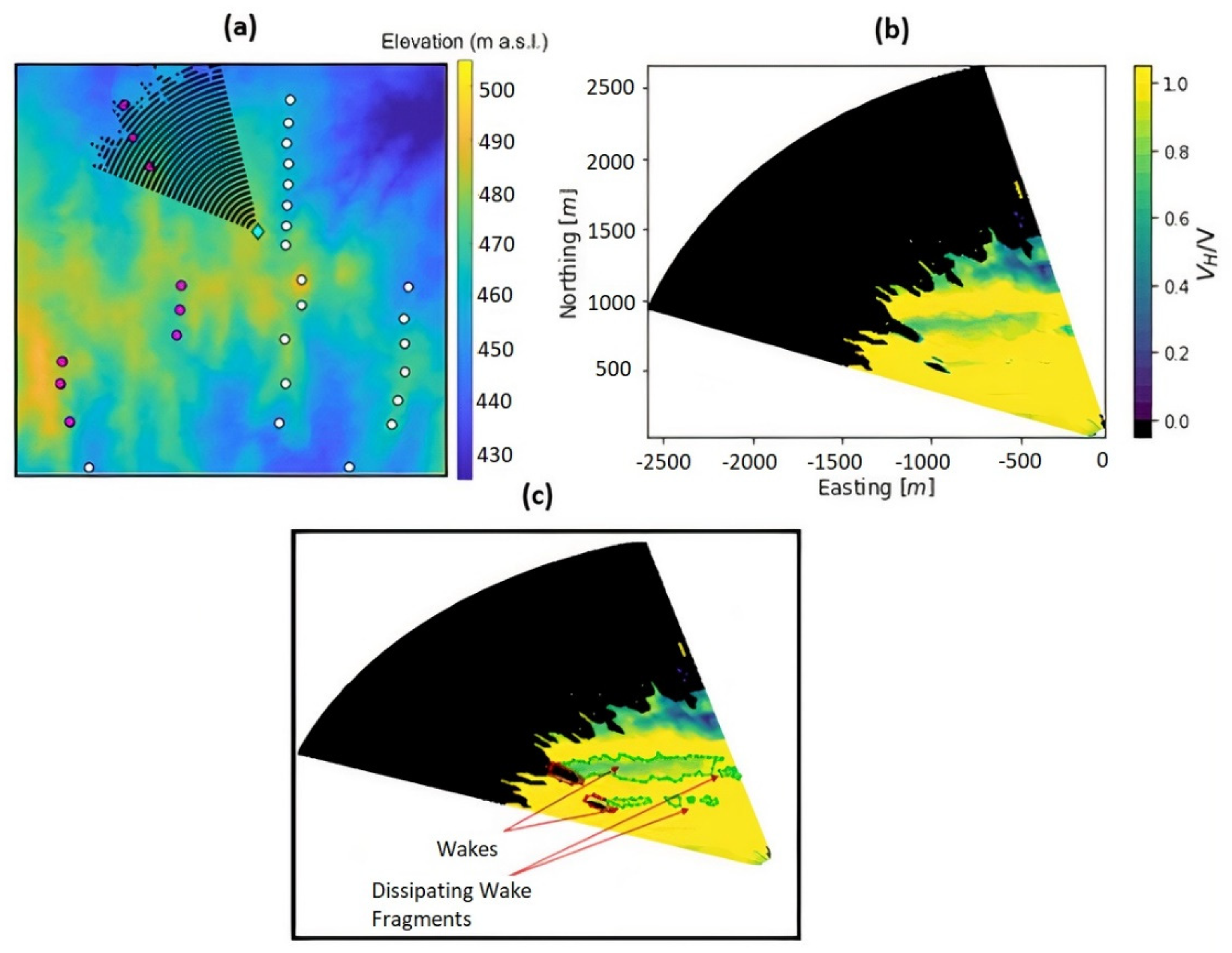
Figure 5.
(a) Area covered by the scan depicted in (b,c), showing the target (magenta) and captured (white) turbines and the lidar location (cyan diamond); (b) scan flow field values normalized by the calculated bulk wind velocity per scan; (c) example of annotations for wakes and wake fragments (green) and wind turbines (red) in a training scan. Scan parameters: arc scan, captured on 3 July 2018, 01:10 UTC, elevation angle = 1.5°, azimuth angle , azimuthal resolution 1°, range gate 50 m, 55 s accumulation time.
The wide variety of azimuth angles encompassed by scans in the subsets result in a high coverage of the flow field; wakes were captured from each turbine depicted in Figure 1. These scans collectively include nearly 1500 instances of wakes and wake fragments and nearly 1000 hard-target returns attributed to turbines obstructing the flow field i.e., two classes (types of objects). Both class annotations are depicted in Figure 5. All data subsets (testing, validation, training) frequently included multiple wake or wake fragment instances per scan. Depending on the arc scan region (i.e., A, B, C or D), a single scan can cover between 2 (Region D) and 10 wakes (Region B).
2.5. About Mask R-CNN: CNN Model, Backbone, and Training Configurations
Mask R-CNN detects and segments (per-pixel object identification) instances of objects within images (network architecture is discussed in [36]). An extension of Faster R-CNN, Mask R-CNN takes inputs of images and their annotations and outputs predictions for object classifications, bounding boxes, confidence in predictions and segmentation masks (thus, segmentation masks represent the entire shape of the object, pixel-by-pixel, as predicted by the CNN) [41,42]. Mask R-CNN operates broadly as follows: the network’s region proposal network (RPN) identifies regions of interest and proposes bounding boxes for identifiable objects within the image. Following this, bounding boxes are refined and the network predicts the object class probabilistically while producing binary pixel masks for regions of interest. Through this process, the image is input through multiple unique layers that process and understand the input, such as convolutional layers (applying a filter to input arrays to create feature maps) and pooling layers (reducing the dimensionality of input data). The final CNN output contains bounding boxes and binary masks of the original input dimensions in pixels for each object detected.
Improvements to the RPN used here include implementation of a feature pyramid network (FPN) as the network backbone [43] (thus, the FPN is integrated into the CNN prediction process). The FPN extracts feature maps from images through a series of convolutional layers and inputs those feature maps to the CNN’s RPN. With a FPN backbone, features are extracted from images with better accuracy and efficiency, with particular robustness in identifying features of varying sizes. Utilization of a FPN backbone results in higher object detection and instance segmentation accuracy than when a backbone is not employed; thus, this work explores the implementation of the ResNet-101 FPN backbone utilized in tandem with Mask R-CNN when detecting and segmenting wakes in scans. We chose the ResNet-101 FPN because of its high accuracy and efficiency in instance segmentation when compared to other backbones [43].
Model weights were initialized with weights from the same Mask R-CNN model with a ResNet-101 FPN backbone trained on the COCO dataset [44] through transfer learning (initializing a model’s weights with weights produced from pre-training the model on a different dataset). Transfer learning has been shown to improve model accuracy and reduce training time [45,46].
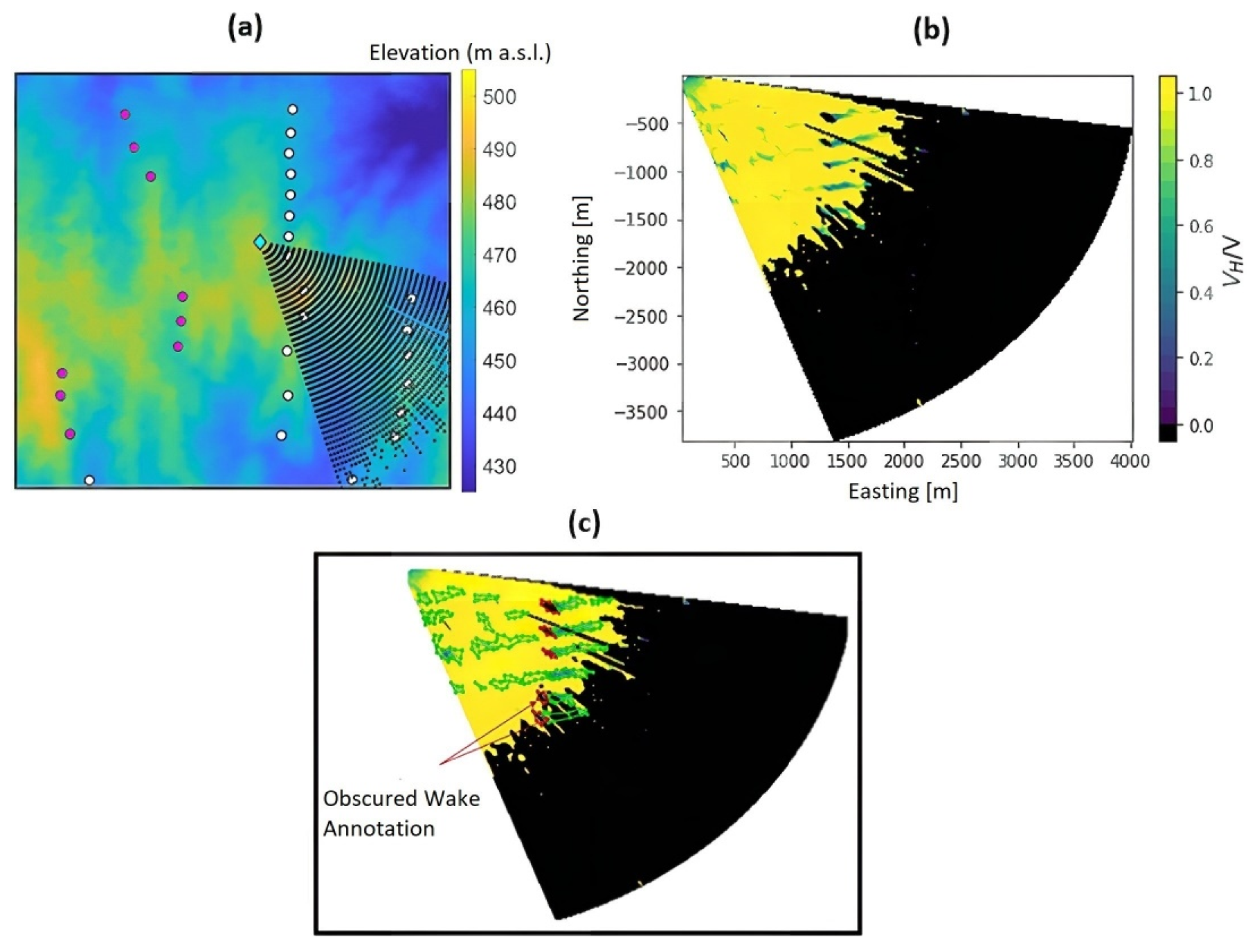
Prior to application of the CNN, all 354 scan images (each with multiple instances of wakes/wake fragments; approximately 1000 wakes in total are included in the dataset) were manually annotated for wakes and wake fragments, and the resulting annotations were utilized in each step of the CNN implementation process: training input, validation input (to reduce over or underfitting) and model accuracy evaluation for the testing subset. Figure 5 and Figure 6 give examples of training annotations, with wakes and wake fragments annotated in green, and visible flow disturbances resulting from the presence of turbines annotated in red. Wakes and wake fragments with obscured velocity data because of CNR filtering are subjectively annotated in order to produce a coherent wake mask (Figure 6). Through this annotation methodology, the CNN was trained to identify wakes and to output their geometries when wakes are present but obscured by missing data, as is common for arc scans that utilize large azimuth ranges to capture multiple rows of turbines (as seen in Figure 6).

Figure 6.
(a) Area covered by the scan depicted in (b,c), showing the target (magenta) and captured (white) turbines and the lidar location (cyan diamond); (b) scan flow field values normalized by the calculated bulk wind velocity per scan; (c) example of the annotation of obscured wakes as a result of quality control procedures. Scan parameters: arc scan, captured on 3 July 2018, 11:41 UTC, elevation angle = 1.0°, azimuth angle , azimuthal resolution 1°, range gate 50 m, 62 s scan time.
CNN parameters were optimized through error minimization in the training subset and then evaluated for overfitting using the validation subset. The testing subset was repeatedly presented to the CNN (i.e., there are a number of iterations) and the results were used diagnostically in training(i.e., the reduction in error (loss) as the model learns the patterns through iteration). Loss indicates the fidelity of the model’s object identifications; if a model identifies/segments an object perfectly, the loss is zero. Mask R-CNN specifically assesses loss for object classification (deciding what the objects are, and classifying them as turbine or wake), object localization (drawing a bounding box around objects in the image to identify their location within the image) and instance segmentation (returning per-pixel segmentation masks for each object detected in the image). Further, Mask R-CNN assesses loss within the RPN for object classification and localization. These losses were summed to calculate total loss as the model trained. The validation dataset can be assessed for model performance alongside the training set when making predictions for a dataset it has never seen. Thus, if the validation set loss levels out or increases while the training set loss continues to decrease, the model is likely overfitting to the data. The validation vs. training loss curve for the model indicates that, for the training configuration employed, around 3000 iterations (the steps at which the neural network updates its weights after learning from training images) are adequate for avoiding overfitting while producing accurate results (Figure 7). The training batch size was kept at 2 images per iteration. Utilizing a graphics processing unit (GPU), computational time for processing each scan image in the validation subset varied from around 0.2–0.7 s, depending on the GPU utilized.
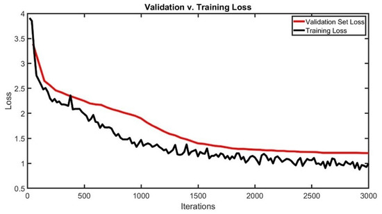
Figure 7.
Example model diagnostic showing the validation and training loss curves as a function of model iterations. The training loss curve shows the rate of model learning as a function of the number of learning cycles (iterations). High loss values indicate higher classification and identification errors. The validation–loss curve highlights the generalizability of the model (indicating extent of overfit or underfit to the dataset when training).
After the CNN was trained on the training and validation subsets of scans and the loss curve was analyzed for model quality, the testing subset was input into the CNN to evaluate its ability to correctly identify and characterize wakes and wake shapes. The testing subset was subject to visual inspection and annotated to provide a measure of ground truth. After the CNN identified wakes and output masks for each, masks were compared to ground truth annotations to obtain model accuracy metrics.
2.6. Model Accuracy Metrics and Criteria
The testing dataset comprised 59 scan images chosen at random that contained approximately 300 instances in total of wakes and wake fragments. Model success is dependent on both wake characterization and wake identification success when compared to subjective annotation. Areas of intersection (in pixels) of masks and subjective annotations are denoted as the intersection over union (IoU). Thus, each wake mask output by the CNN was associated with a unique IoU value when compared to subjective annotation. For the proof of concept, the IoU needed for a successful wake mask was 0.6 or greater (60% of the CNN mask’s area in pixels intersects the subjectively annotated wake’s area in pixels, Table 1).

Table 1.
Criteria for success and failure when evaluating wake mask results from the convolutional neural network (CNN).
Wakes with obscured shapes because of CNR filtering were evaluated separately with the same criteria for failure and success. Successes and failures were calculated per unique wake, and thus each scan can produce multiple instances of successes and failures, depending on the number of wakes and masks observed. All success rates were calculated through the following expression:
Occasionally, wake masks returned by the model identify nested wakes, which occur when one wake mask is within another. Seven percent of wake masks returned for the full resolution testing set contained nested masks. Nested model predictions for bounding boxes and masks are commonly seen in image processing applications and can be mitigated through adjusting parameters during training (such as adjusting non-maximum suppression parameters [47]). For this use case, it is possible that a small number of nested predicted wakes were unavoidable because of the nature of velocity contours and the coarse spatial resolution of the scans. Further, when analyzing the nested wakes subjectively, their aggregated mask was often sufficient when identifying the wake and wake fragment geometries. Consequently, nested wakes are treated as single entities herein and counted in only one IoU estimation.
2.7. Sensitivity to Scan Resolution and Flow Conditions
As lidar technology evolves and scan resolutions vary per campaign, it is pertinent to examine how the model, and the subsequent wake characteristics, are affected when applied to lower resolution scans. To assess the model’s performance under a variation in range gate resolution, each of the radial velocity fields in each scan in the testing dataset was down-sampled such that every other value was removed, reducing the range gate resolution from 50 m to 100 m. Wake characteristics were then calculated for down-sampled scans and compared to full resolution scans.
As wake geometries are dependent on atmospheric conditions and flow field velocities, variations in wake characteristics and model accuracy were assessed by classifying the atmospheric conditions under which each scan was performed (Table 2). Scans were defined as “low” wind speed if the median horizontal wind speed is <9 ms−1 in the 59 testing scans. Scans captured during lower velocity conditions result in higher thrust coefficients, which yield relatively larger magnitude wakes. In addition, lower velocities are most often associated with higher turbulence intensities [48]. Scans performed during the daytime (8 a.m.–8 p.m., local time) are placed into a class of unstable stratification.
Table 2.
Atmospheric classes used in the analysis of varying scan resolution on wake characteristics.
After wakes and wake fragments in each atmospheric class were identified for both scan image resolutions (full, half) based on the threshold for IoU, three wake characteristics were analyzed: asymmetry, length and width. These metrics are defined below, and depend on the characterization of the wake or wake fragment’s skeleton, which is otherwise known as the medial axis of the object. The skeleton (the mathematical process to calculate the skeleton is described in detail in [49]) is a simplified shape representation used often in image processing applications and is utilized herein as an approximation for the geometric wake centerline (Figure 8).

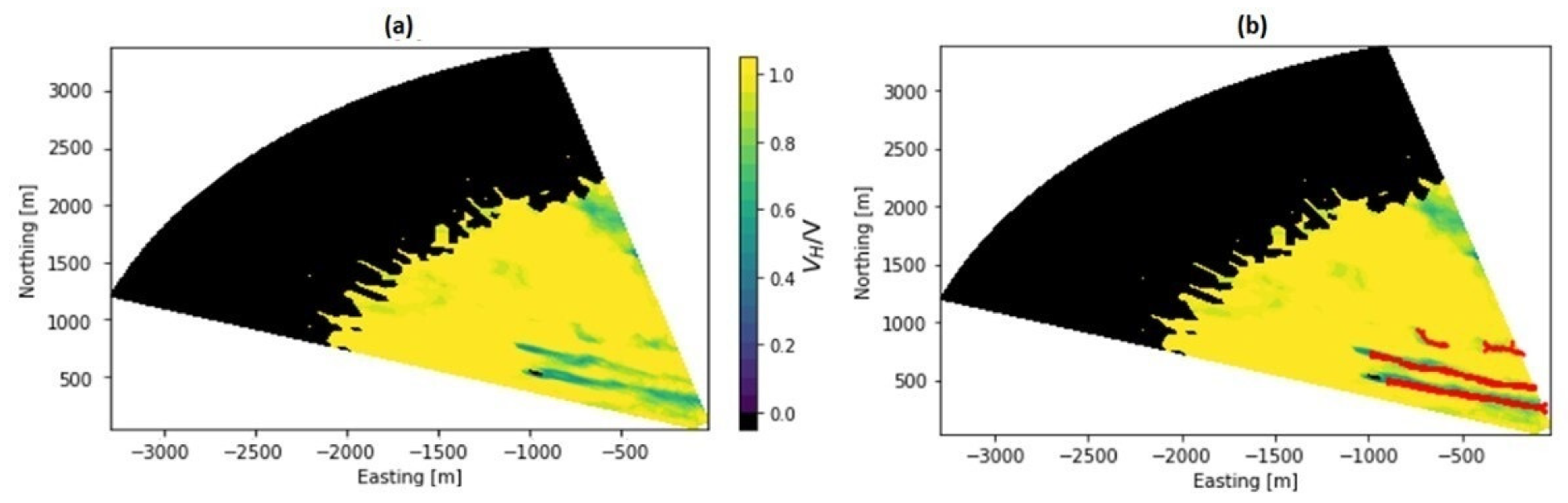
Figure 8.
(a) Scan example; (b) wake skeletons (medial axes) for wakes and wake fragments present in the scan (red). Scan colored by flow field horizontal velocities () normalized by calculated bulk wind speed (V). Scan parameters: arc scan, captured on 11 September 2018, 02:57 UTC, elevation angle = 3.5°, azimuth angle , azimuthal resolution 1°, range gate 50 m, 55 s scan time.
Width: In this analysis, wakes propagate along an approximate west–east axis, so an approximation of the mean wake width (perpendicular to the skeleton) was computed as the sum of the number of pixels in the y-direction (south-north) that are enclosed by the wake boundary at a given point along the skeleton divided by the total number of points along the skeleton;
Asymmetry: After the wake/wake fragment’s skeleton was identified, the pixels above and below the skeleton (in the north–south [y] direction) were projected to two histograms, where each bin represents the point along the skeleton, and the histogram width is the number of pixels above (or below) the skeleton. Each projected histogram thus represents the distribution of pixels in the y direction along the length of the skeleton, with one histogram representing the distribution of pixels above the skeleton and one histogram representing the distribution of pixels below. The correlation of these projected histograms was then assessed through evaluation of the Pearson correlation coefficient. A high correlation coefficient corresponds to high north–south symmetry along the skeleton (approximate wake centerline), i.e., the width of the pixels in the upper half of the wake correlate with the width of the pixels in the lower half of the wake for each point along the skeleton;
Length: The wake length was assessed through calculating the distance between the easternmost and westernmost wake skeleton locations for east–west propagating wakes, or the westernmost and easternmost wake skeletons for west–east propagation cases.
3. Results
3.1. CNN Model Performance
The CNN exhibits a 95.65% success rate in identifying and outputting sufficient masks for the wind turbine wake shape when compared to the ground truth annotation in the independent test sample of 59 scans (Table 3). For wake fragments, the model exhibits a 77.53% success rate. In cases where the wind turbine wakes are embedded in a highly heterogeneous data field as a result of the removal of many data points because of CNR filtering, the success rate decreases to 87.18%. However, all four wake fragments that are embedded in a highly heterogeneous data field as a result of the removal of many radial velocity estimates because of CNR filtering are correctly identified.
Table 3.
Success rates for wake and wake fragment identification and characterization for the Mask region-based CNN model with ResNet-101 feature pyramid network backbone.
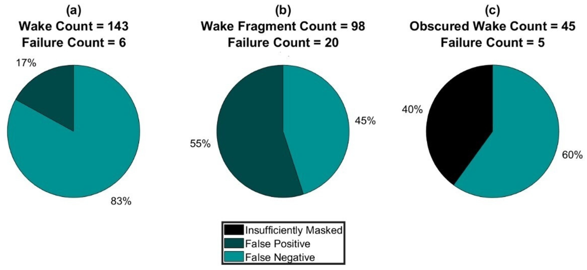
The most common mode of failure for the CNN is a false negative—i.e., there is a wake or wake fragment in the scan and the model does not identify it as an object at all (Figure 9). The second most common mode of failure is returning a false positive—i.e., a non-wake (such as a wind turbine) structure is identified as a wake. False positives may also be attributed to uncertainties in radial velocity measurements that arise from misalignment between the lidar line of sight and the wind direction [50]. Failure associated with low IoU (incorrect wake shape) is very rare (one case). This indicates that, when the model does correctly identify a wake or wake fragment, it is highly skilled at returning the correct mask for the structure, especially if the structure is not obscured by data removal. Although more than three-quarters of wake fragments are captured by the model, they are associated with a higher number of false positives that are caused by the model’s sensitivity to other low-velocity flow structures in the scans.
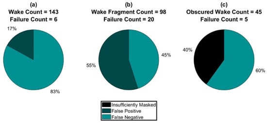
Figure 9.
Analysis of model failure modes when identifying and characterizing (a) wakes, (b) wake fragments and (c) obscured wakes. Values are for the testing data subset. Pie charts depict the failure modes as a percentage of total number of failures for fully visible and obscured wakes and wake fragments. Note: only four obscured wake fragments are included in the testing set and all four were identified successfully.
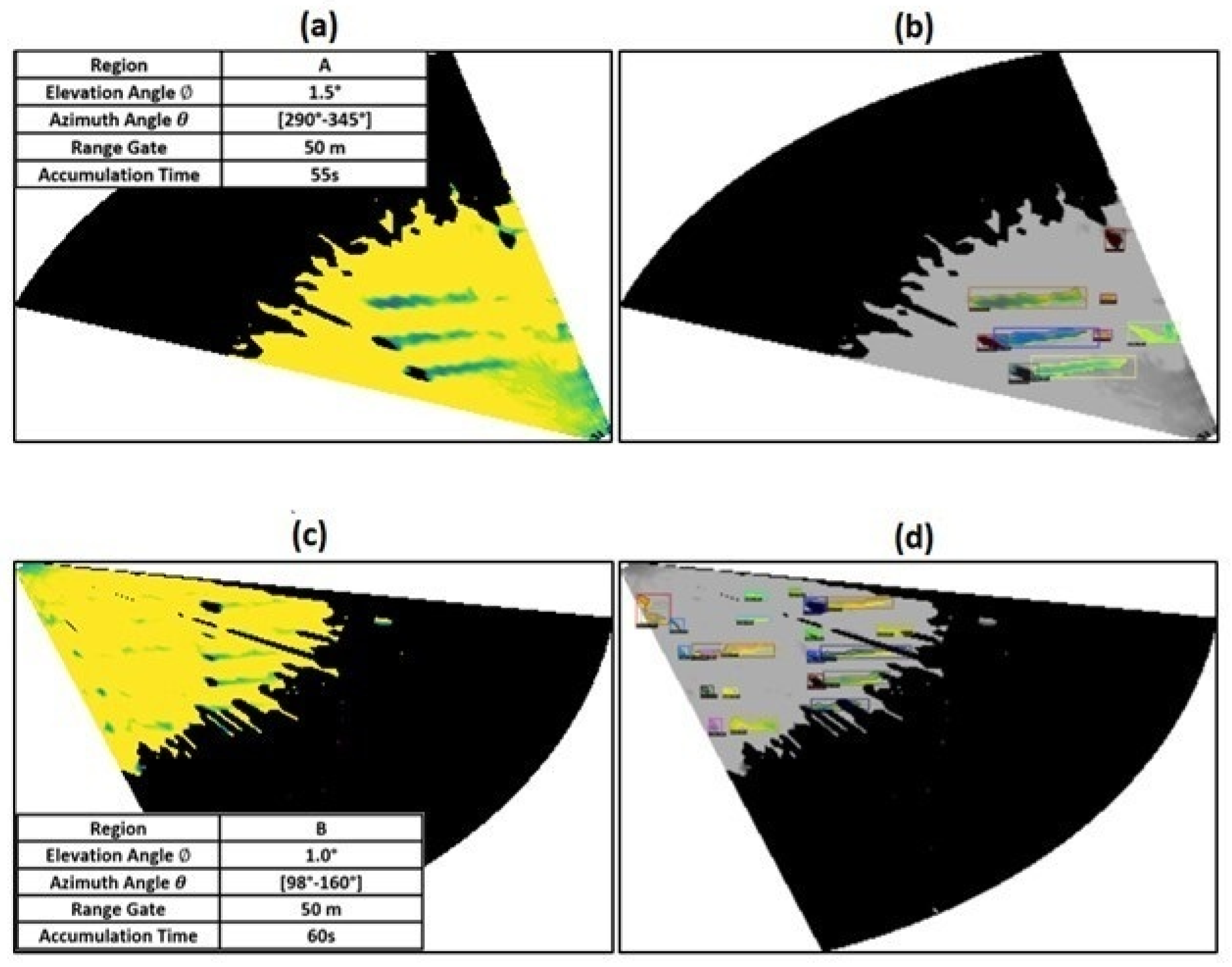
Illustrative examples of wake identification in different scan sectors (see Figure 1b) are shown in Figure 10 and Figure 11. The scan from Region A (northwest) exhibits a correct identification of wakes and wake fragments for a data-dense flow field (few velocity values are removed by the CNR screening) (Figure 10a,b). The CNN differentiates between the region of low velocity in the lower right corner of the scan and the wake that is near it. Further, the CNN is able to successfully identify and mask the complex wake fragment in the scan. The scan from Region B exhibits a larger area scanned than that of Region A because of a higher maximum range distance, which reduces the visibility of the wakes in the image (Figure 10c,d). Regardless, the CNN is able to successfully identify the wakes and wake fragments and output successful masks, even when wind turbine wakes are close to regions with missing radial velocity estimates.

Figure 10.
Comparison of (a,c) input scan and (b,d) model output when identifying wakes, wake fragments and obscured wakes. Scan parameters for (a,b): arc scan, captured on 11 September 2018, 04:51 UTC, elevation angle = 1.5°, azimuth angle , azimuthal resolution 1°, range gate 50 m, 55 s accumulation time. Scan parameters for (c,d): arc scan, captured on 3 July 2018, 07:55 UTC, elevation angle = 1.0°, azimuth angle , azimuthal resolution 1°, range gate 50 m, 60 s scan time. Mask colors are unique and represent individual wakes and wake fragments detected by the model.

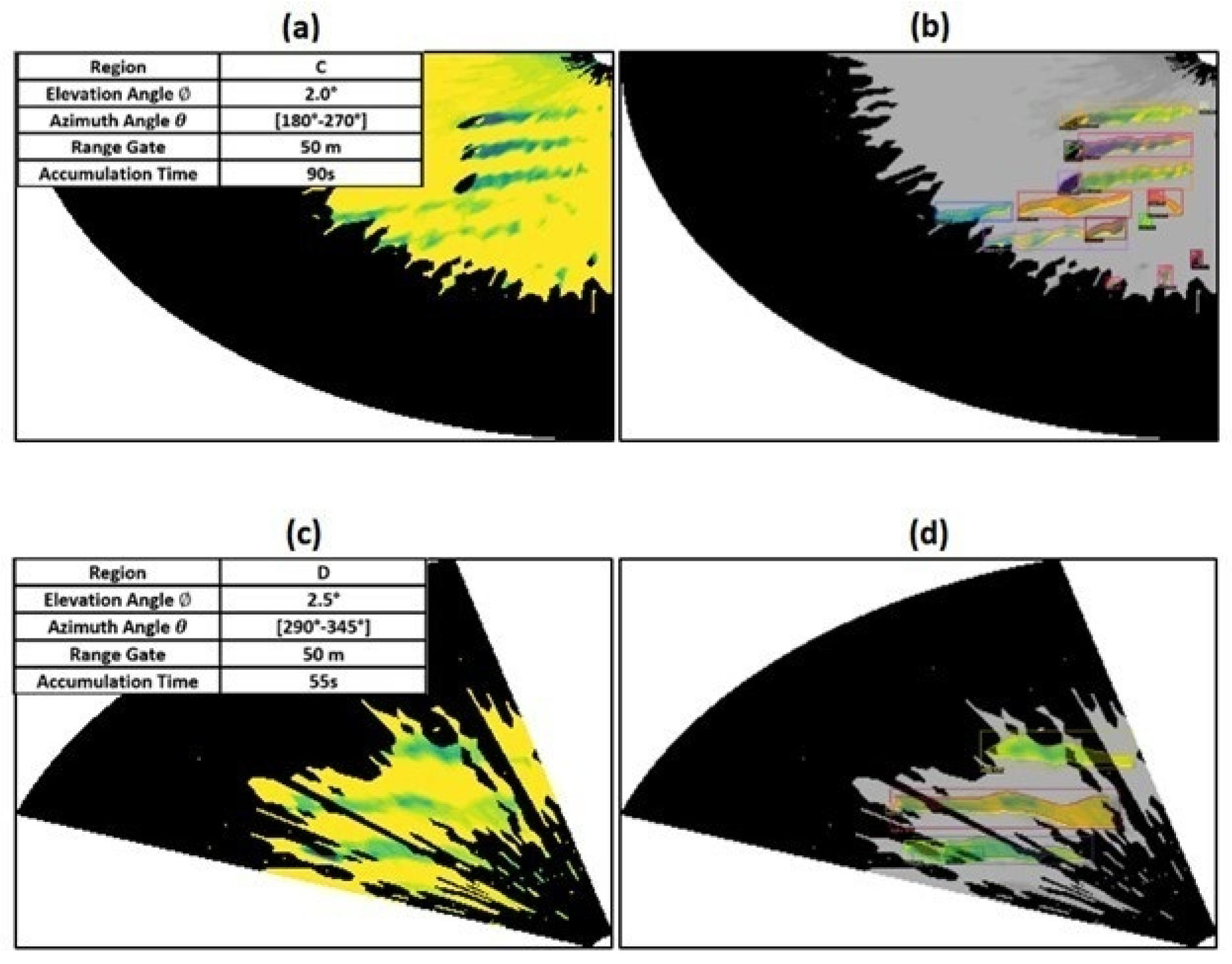
Figure 11.
Comparison of (a,c) input scan and (b,d) model output when identifying wakes, wake fragments and obscured wakes. Scan parameters for (a,b): arc scan, captured on 2 September 2018, 04:50 UTC, elevation angle = 2.0°, azimuth angle , azimuthal resolution 1°, range gate 50 m, 90 s accumulation time. Scan parameters for (c,d): arc scan, captured on 12 September 2018, 04:24 UTC, elevation angle = 2.5°, azimuth angle , azimuthal resolution 1°, range gate 50 m, 55 s scan time.
The example scans from Regions C (northwest but over a smaller area than Region A, see Figure 1b) and D (southeast) also illustrate cases with a correct identification of wakes and wake fragments from scans with richly defined flow fields, and those where the CNR filtering has yielded a more complex and heterogeneous data field (Figure 11).
3.2. Model Sensitivity to Image Resolution
When the testing scans are down-sampled to half resolution (from a range gate of 50 m to an effective range gate of 100 m) and input into the CNN for wake identification and characterization, the success rate declines. However, the model remains skillful in identifying and correctly masking wakes when present in scans, with a 92.19% success rate (Table 3). This down-sampling exercise is meant to indicate whether large-area scans covering a large portion of an entire wind plant can be used to detect the approximate location and extent of individual wakes.
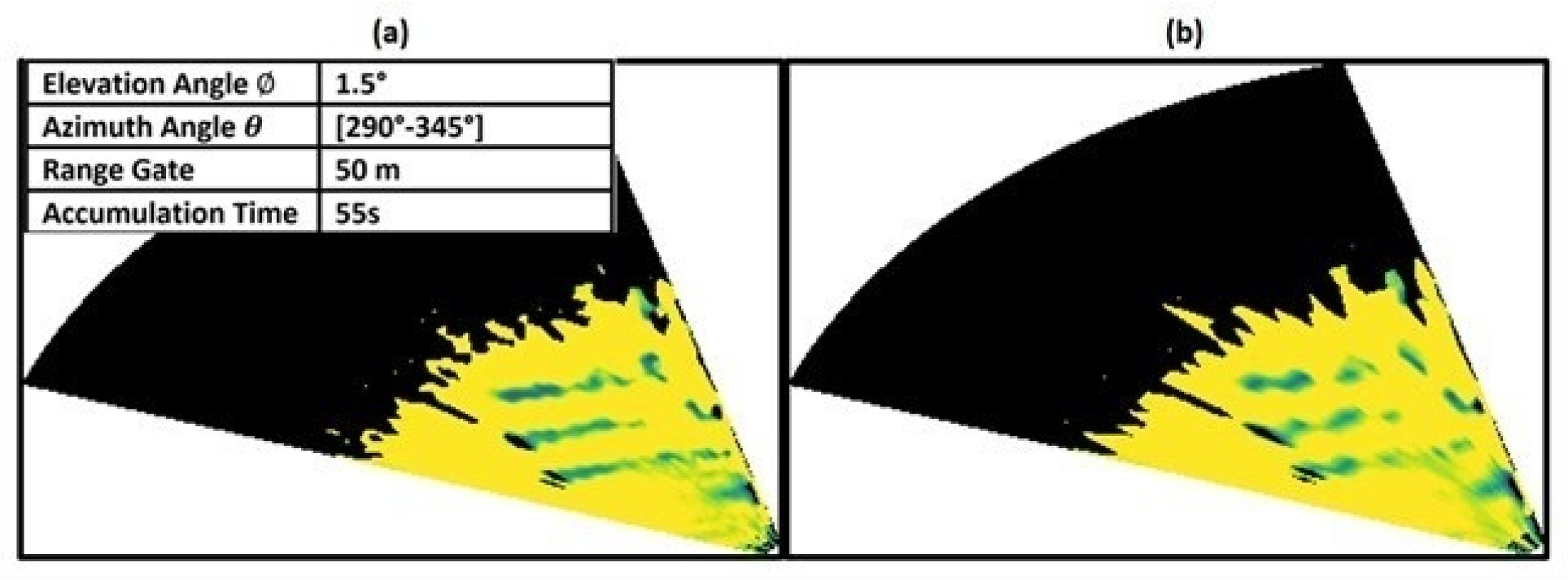
Down-sampling the scans results in an increase in subjectively identifiable wake fragments (111 wake fragments under half-resolution, 98 under full resolution). This is illustrated by Figure 12, where all three wakes in the full resolution scan are more fragmented when subjected to half-resolution down-sampling. When considering the failure modes for wake fragments under half-resolution, 71% of model failures under half-resolution are attributed to false negatives (the CNN is unable to detect the wake fragments when they are present). Thus, the high success rate for wake fragment identification under full resolution is likely attributed to specific flow patterns that differentiate wake fragments from other local, low-velocity turbulent flow. The number of insufficiently masked wakes (IoU < 60%) increases, with insufficient wake masks representing 20% of the model failure.
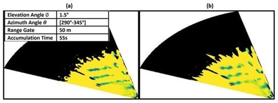
Figure 12.
(a) Full-resolution scan image; (b) half-resolution scan image. The reduction in resolution results in increased number of wake fragments and modified wake characteristics. Scan parameters: arc scan, captured on 11 September 2018, 05:14 UTC, elevation angle = 1.5°, azimuth angle , azimuthal resolution 1°, range gate 50 m, 55 s accumulation time.
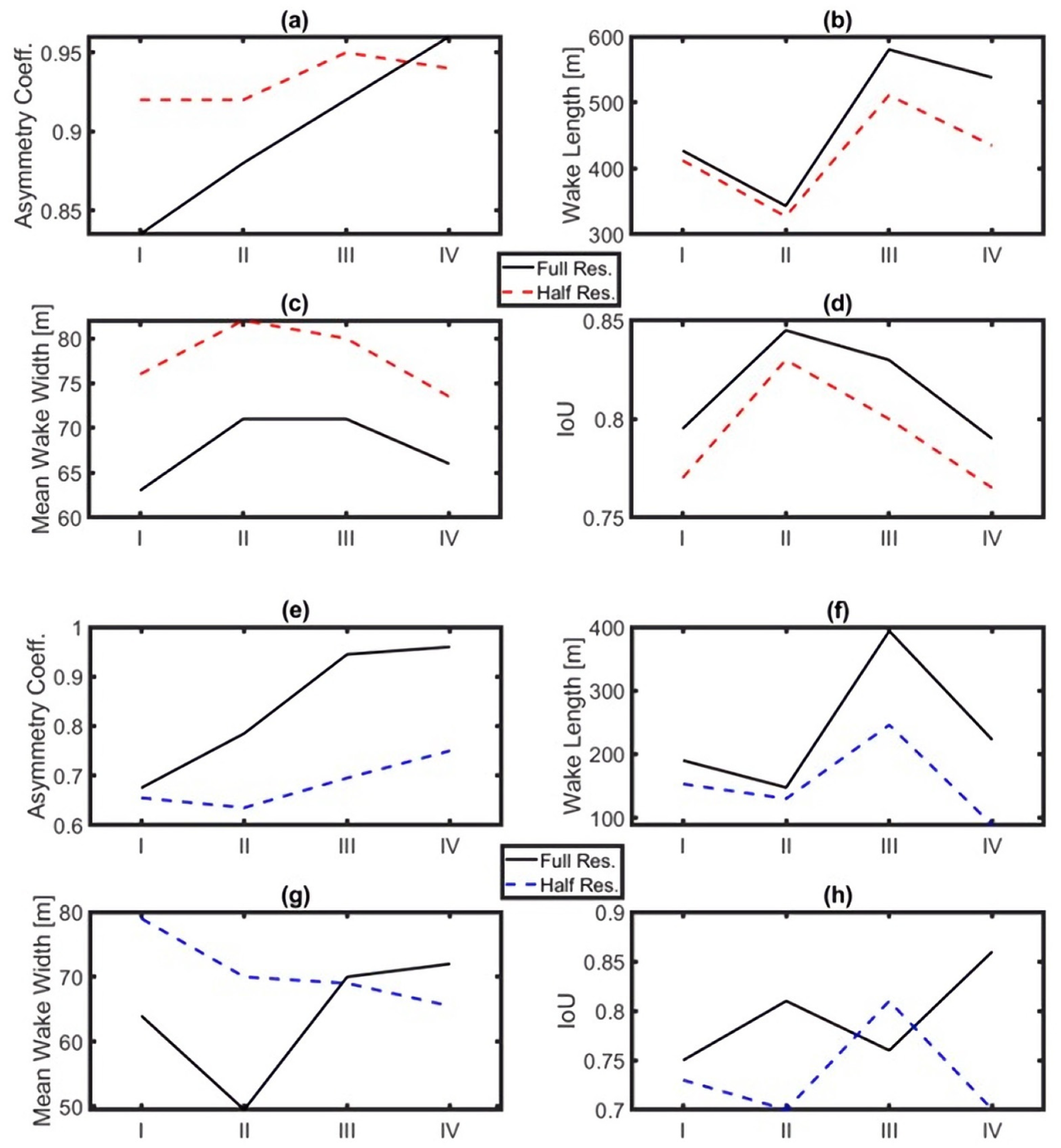
Wake asymmetry, width and length for all complete (boundaries completely included in the scan) wakes and wake fragments that exhibit adequate IoU when compared to subjective annotation () exhibit some sensitivity to input data resolution, and there is a clear reduction in IoU for the half-resolution scans irrespective of the prevailing atmospheric conditions (Figure 13). Down-sampling results in an increase in the calculated median wake width for all scans (Figure 13). Further, the normalized wind fields exhibit wakes that become more irregularly shaped, indicated by an increasing asymmetry (Figure 12). Note that these results are reasonable, as a spatial resolution of 100 m is rather coarse for the 90-m diameter wind turbines generating the wakes. For each inflow class (Table 2), the sample size of full and complete wakes that are accurately characterized by the CNN is greater than 20. Although wake characteristics exhibit marked differences according to atmospheric conditions, the overall relative differences in the wake width, length and asymmetry magnitude between each atmospheric class are similar for full and half resolutions. The IoU varies between classes of atmospheric conditions in a similar manner to wake width, with both being highest under daytime low wind speeds and nighttime high wind speeds. Conversely, the wake length is largest for the higher wind speeds in both daytime and nighttime scans, and smallest for low wind speeds and daytime conditions, when unstable stratification is expected to erode wakes more rapidly (Figure 13). Intra-class patterns in wake width generally follow trends in the model IoU, potentially indicating that the model accuracy is more sensitive to wake width than wake length. This could be attributed to the existence of a minimum threshold of wake width or length needed for wakes to be visibly detected; in this case, it is likely that wakes will have an adequate length to be detected when compared to width (which is a numerically smaller dimension, as evidenced in Figure 13).
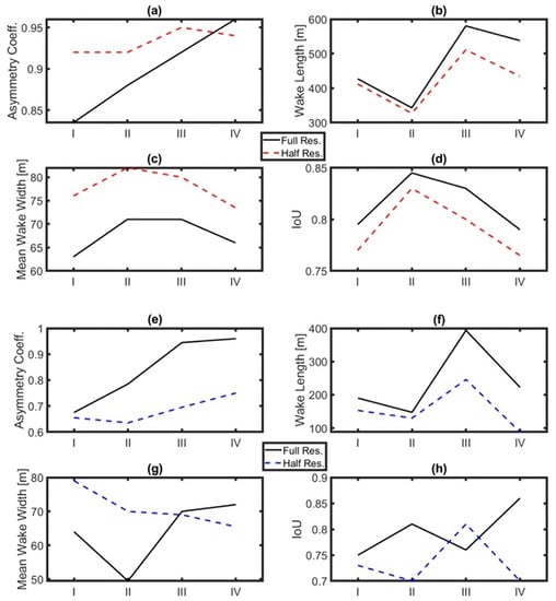
Figure 13.
Model performance in characterizing wakes (a–d) and wake fragments (e–h) for each inflow class defined in Table 3 (horizontal axis) at full (solid line) and half resolution (dashed line). Wake and fragment characteristics include asymmetry (a,e), length (b,f) and width (c,g) and are given as the median of all values. The characteristic width of a given wake is given by the mean value along its length. Model success metric intersection over union (IoU) is given in (d,h).
Wake fragment characteristics are more susceptible to change under a reduction in resolution than wakes. Generally, the wake and wake fragment asymmetry decrease across classes, with Class I exhibiting the lowest median asymmetry coefficients in the range of 0.65–0.925 (and thus highest asymmetry). Thus, Class I wake and wake fragments are characterized by a relatively high asymmetry, fast wake recovery and lower model accuracy rates. It is possible that this may be attributed to the complex terrain, although further investigation is warranted in order to verify this. For lower wind speeds and stable, nighttime conditions, it is possible that winds and wakes are the mostly strongly coupled with the underlying terrain. Given that conditions for Class I are approximated as stable with a lower speed inflow, these wake characteristics are consistent with a priori expectations. Decreased the stability in Class II when compared to Class I results in Class II having the lowest median wake length. Note that the sample sizes reported here are lower than the ensemble wake fragment sample size reported in Figure 10 because of the requirements that (i) the wake fragments be complete (as it is impossible to fully characterize a wake fragment if its entirety is not included in the scan) and that (ii) characterization be applied to wake fragments sufficiently identified (as described by the IoU criterion for CNN prediction and ground truth) by the CNN. Wake characteristics observed in Class III also follow a priori expectations—the wake recovery is the slowest for this class, which is marked by increased inflow speeds and approximately stable conditions, as indicated by the time of day (nighttime). Class IV, characterized by higher inflow speeds and decreased stability, exhibits the lowest accuracy in wake and wake fragment identification, which may be attributed to an increase in the length scale of background flow structures and an associated amplification of false positive detections. Further, because lidar measurement uncertainties for arc scans scale with turbulence intensity, it is possible that the higher uncertainties associated with an increased turbulence contribute to a lower accuracy rate in Class IV [50]. Results of wake characteristics from each class and their agreement with a priori expectations further indicate CNN accuracy in determining wake characteristics and outputting reasonable wake masks.
4. Discussion and Conclusions
We implemented a Mask R-CNN model with a ResNet 101 FPN backbone for wake characterization and identification in complex terrain from lidar arc scans. The lidar data were collected during a campaign spanning July 2018–December 2018 (inclusive) at a wind farm in the U.S. Pacific Northwest. The dataset contains a wide variety of experimental parameters, such as range gate, resolution, number of wakes captured and scanning time. The variety of the dataset makes it ideal for evaluation of the model under a wide range of experimental parameters. A subset of 354 arc scans with approximately 1000 wind turbine wakes is employed in this proof-of-principle analysis. Two-thirds of the scans are used for model training, whereas the other one-third is split evenly among model validation and testing.
Many of the scans contain regions of missing velocity measurements as a result of CNR filtering, and the wakes are in various stages of formation and dissipation because of terrain complexity, resulting in wakes with multiple fragments throughout the flow field. These fragments and wakes are often asymmetric, a geometric quality that presents challenges for current wake identification and characterization methods. Thus, common techniques for wake characterization and identification are difficult to implement for the dataset.
The CNN applied here is successful regardless of these difficulties, exhibiting high skill in identifying wakes and dissipating wakes from full and lower resolution lidar arc scan images. The success rate for wake identification from full resolution scan images in which wakes are present is 95%. The most common failure mode for full wind turbine wakes is a false negative. In this case, the model does not identify a wake when one is present. The most common error in identifying dissipated wake fragments within the scans is a result of false positives, which are defined as the model identifying a flow field structure as a dissipating wake fragment when it is not. When the scan resolution is degraded by removing data from every other range gate, an increase in false negatives is observed when identifying dissipating wake fragments. This indicates that wake fragment flow contours under full resolution are unique, and that the CNN utilizes specific flow patterns to differentiate between wake fragments and other low-velocity turbulent flow. However, the model still exhibits skill in identifying wakes under reduced resolution, with a success rate of 92%. Although reductions in the range gate alter wake characteristics numerically, when the scans are clustered by prevailing wind speed and atmospheric stability, the behavior of wake characteristics between each group is conserved. Further, median wake characteristics per group (grouped by inflow velocity and time of scan collection to provide a broad metric for atmospheric stability) are broadly consistent with a priori expectations, further indicating model accuracy and applicability.
Results indicate that the Mask R-CNN has a wide applicability to a range of challenges in wind energy science, including improving existing simulation tools for wakes in complex terrain, improving knowledge of wake dynamics in complex terrain, enabling real-time wake identification and characterization from remote sensing data and assisting in condition monitoring. Future work will include an implementation of Mask R-CNN models with a higher accuracy (Scoring Mask R-CNN, Cascade Mask R-CNN) and will involve the fine-tuning of model training parameters. Uncertainties due to the flow field reconstruction method utilized will be explored further. For example, scans with wind directions close to normal to the scanning direction were not filtered out in this study. Although flow reconstruction under these conditions may result in flow field errors, the inclusion of these scans in the training dataset may be helpful in terms of training the CNN to recognize wakes even in these conditions. These uncertainties, as well as the uncertainties in calculating the bulk wind direction per scan for the purpose of reconstructing the flow field, will be further investigated. New wake classes may be implemented when training the model to enable the detection of wake interactions (wakes mixing with each other) and to increase the amount of training data.
Author Contributions
J.A.A. developed the concept and analysis strategy with input from E.W.Q., R.J.B., S.C.P., P.D. and M.D., J.A.A. ran the analysis and generated the figures. M.D. performed the field campaign with the scanning lidar. J.A.A. wrote the manuscript with input from S.C.P., R.J.B., E.W.Q., M.D. and P.D. All authors have read and agreed to the published version of the manuscript.
Funding
This work was supported by the National Science Foundation Graduate Research Fellowship Program (DGE-1650441), the U.S. Department of Energy (DoE) (DE-SC0016605) and the National Offshore Wind R&D Consortium (147505). This work was authored in part by the National Renewable Energy Laboratory, operated by Alliance for Sustainable Energy, LLC, for the U.S. Department of Energy (DOE) under Contract No. DE-AC36-08GO28308. Funding provided by the U.S. Department of Energy Office of Energy Efficiency and Renewable Energy.
Acknowledgments
J.A.A. is grateful to NREL for summer internships under which this research was developed. We thank Ryan Dela for providing access to the scanning lidar.
Conflicts of Interest
The authors declare no conflict of interest.
Disclaimer
The views expressed in the article do not necessarily represent the views of the DOE or the US Government. The US Government retains and the publisher, by accepting the article for publication, acknowledges that the US Government retains a nonexclusive, paid-up, irrevocable, worldwide license to publish or reproduce the published form of this work, or allow others to do so, for US Government purposes.
References
- Eggers, A.J., Jr.; Digumarthi, R.; Chaney, K. Wind shear and turbulence effects on rotor fatigue and loads control. J. Sol. Energy Eng. 2003, 125, 402–409. [Google Scholar] [CrossRef]
- Hand, M.M.; Kelley, N.D.; Balas, M.J. Identification of wind turbine response to turbulent inflow structures. Fluids Eng. Div. Summer Meet. 2003, 36967, 2557–2566. [Google Scholar]
- Barthelmie, R.J.; Hansen, K.; Frandsen, S.T.; Rathmann, O.; Schepers, J.G.; Schlez, W.; Phillips, J.; Rados, K.; Zervos, A.; Politis, E.S.; et al. Modelling and measuring flow and wind turbine wakes in large wind farms offshore. Wind Energy 2009, 12, 431–444. [Google Scholar] [CrossRef]
- Lee, S.; Churchfield, M.; Moriarty, P.; Jonkman, J.; Michalakes, J. Atmospheric and wake turbulence impacts on wind turbine fatigue loadings. In Proceedings of the 50th AIAA Aerospace Sciences Meeting Including the New Horizons Forum and Aerospace Exposition, Nashville, TN, USA, 9–12 January 2012; p. 540. [Google Scholar]
- Quon, E.W.; Doubrawa, P.; Debnath, M. Comparison of Rotor Wake Identification and Characterization Methods for the Analysis of Wake Dynamics and Evolution. J. Phys. Conf. Ser. 2020, 1452, 012070. [Google Scholar] [CrossRef]
- Doubrawa, P.; Barthelmie, R.J.; Wang, H.; Pryor, S.C.; Churchfield, M.J. Wind turbine wake characterization from temporally disjunct 3-d measurements. Remote Sens. 2016, 8, 939. [Google Scholar] [CrossRef] [Green Version]
- Espana, G.; Aubrun, S.; Loyer, S.; Devinant, P. Spatial study of the wake meandering using modelled wind turbines in a wind tunnel. Wind Energy 2011, 14, 923–937. [Google Scholar] [CrossRef]
- Barthelmie, R.J.; Pryor, S.C. Automated wind turbine wake characterization in complex terrain. Atmos. Meas. Tech. 2019, 12, 3463–3484. [Google Scholar] [CrossRef] [Green Version]
- Aitken, M.L.; Banta, R.M.; Pichugina, Y.L.; Lundquist, J.K. Quantifying wind turbine wake characteristics from scanning remote sensor data. J. Atmos. Ocean Technol. 2014, 31, 765–787. [Google Scholar] [CrossRef]
- Herges, T.G.; Maniaci, D.C.; Naughton, B.T.; Mikkelsen, T.; Sjöholm, M. High resolution wind turbine wake measurements with a scanning lidar. J. Phys. Conf. Ser. 2017, 854, 012021. [Google Scholar] [CrossRef] [Green Version]
- Vollmer, L.; Steinfeld, G.; Heinemann, D.; Kühn, M. Estimating the wake deflection downstream of a wind turbine in different atmospheric stabilities: An LES study. Wind Energy Sci. 2016, 1, 129–141. [Google Scholar] [CrossRef] [Green Version]
- Panossian, N.; Herges, T.G.; Maniaci, D.C. Wind Turbine Wake Definition and Identification Using Velocity Deficit and Turbulence Profile. In Proceedings of the 2018 Wind Energy Symposium, Kissimmee, FL, USA, 8–12 January 2018; p. 0514. [Google Scholar]
- Barthelmie, R.J.; Pryor, S.C.; Wildmann, N.; Menke, R. Wind turbine wake characterization in complex terrain via integrated Doppler lidar data from the Perdigão experiment. J. Phys. Conf. Ser. 2018, 1037, 052022. [Google Scholar] [CrossRef] [Green Version]
- Kigle, S. Wake Identification and Characterization of a Full Scale Wind Energy Converter in Complex Terrain with Scanning Doppler Wind Lidar Systems. Ph.D. Thesis, Ludwig-Maximilians-Universität, München, Germany, 2017. [Google Scholar]
- Lio, W.H.; Larsen, G.C.; Poulsen, N.K. Dynamic wake tracking and characteristics estimation using a cost-effective LiDAR. J. Phys. Conf. Ser. 2020, 1618, 032036. [Google Scholar] [CrossRef]
- Stein, H.S.; Guevarra, D.; Newhouse, P.F.; Soedarmadji, E.; Gregoire, J.M. Machine learning of optical properties of materials–predicting spectra from images and images from spectra. Chem. Sci. J. 2019, 10, 47–55. [Google Scholar] [CrossRef] [PubMed] [Green Version]
- Puri, M. Automated machine learning diagnostic support system as a computational biomarker for detecting drug-induced liver injury patterns in whole slide liver pathology images. Assay Drug Dev. Technol. 2020, 18, 1–10. [Google Scholar] [CrossRef] [PubMed]
- Marvuglia, A.; Messineo, A. Monitoring of wind farms’ power curves using machine learning techniques. Appl. Energy 2012, 98, 574–583. [Google Scholar] [CrossRef]
- Clifton, A.; Kilcher, L.; Lundquist, J.K.; Fleming, P. Using machine learning to predict wind turbine power output. Environ. Res. Lett. 2013, 8, 024009. [Google Scholar] [CrossRef]
- Leahy, K.; Hu, R.L.; Konstantakopoulos, I.C.; Spanos, C.J.; Agogino, A.M. Diagnosing wind turbine faults using machine learning techniques applied to operational data. In Proceedings of the 2016 IEEE International Conference on Prognostics and Health Management, Ottawa, ON, Canada, 20–22 June 2016; pp. 1–8. [Google Scholar]
- Zendehboudi, A.; Baseer, M.A.; Saidur, R. Application of support vector machine models for forecasting solar and wind energy resources: A review. J. Clean. Prod. 2018, 199, 272–285. [Google Scholar] [CrossRef]
- Ti, Z.; Deng, X.W.; Yang, H. Wake modeling of wind turbines using machine learning. Appl. Energy 2020, 257, 114025. [Google Scholar] [CrossRef]
- Hecht-Nielsen, R. Theory of the Backpropagation Neural Network. Neural Networks for Perception. 1992, pp. 65–93. Available online: https://www.sciencedirect.com/science/article/pii/B9780127412528500108 (accessed on 20 July 2021).
- Rosenblatt, F. Principles of Neurodynamics: Perceptrons and the Theory of Brain Mechanisms; Spartan Books: Washington, DC, USA, 1961. [Google Scholar]
- Bishop, C.M. Neural Networks for Pattern Recognition; Clarendon Press: Oxford, UK, 1995. [Google Scholar]
- Choi, K.; Fazekas, G.; Sandler, M.; Cho, K. Convolutional recurrent neural networks for music classification. In Proceedings of the 2017 IEEE International Conference on Acoustics, Speech and Signal Processing (ICASSP), New Orleans, LA, USA, 5–9 March 2017; pp. 2392–2396. [Google Scholar]
- Egmont-Petersen, M.; de Ridder, D.; Handels, H. Image processing with neural networks—A review. Pattern Recognit. 2002, 35, 2279–2301. [Google Scholar] [CrossRef]
- Chen, J.L.; Chang, J.Y. Fuzzy perceptron neural networks for classifiers with numerical data and linguistic rules as inputs. IEEE Trans. Fuzzy Syst. 2000, 8, 730–745. [Google Scholar]
- Kryzhanovsky, B.V.; Mikaelian, A.L.; Fonarev, A.B. Vector neural net identifying many strongly distorted and correlated patterns. Inf. Opt. Photonics Technol. 2005, 5642, 124–133. [Google Scholar]
- Milletari, F.; Navab, N.; Ahmadi, S.A. V-net: Fully convolutional neural networks for volumetric medical image segmentation. In Proceedings of the 2016 Fourth International Conference on 3D Vision (3DV), Stanford, CA, USA, 25–28 October 2016; pp. 565–571. [Google Scholar]
- Matsugu, M.; Mori, K.; Mitari, Y.; Kaneda, Y. Subject independent facial expression recognition with robust face detection using a convolutional neural network. Neural Netw. 2003, 16, 555–559. [Google Scholar] [CrossRef]
- Ding, G.; Song, Y.; Guo, J.; Feng, C.; Li, G.; He, B.; Yan, T. Fish recognition using convolutional neural network. In Proceedings of the OCEANS 2017-Anchorage, Anchorage, AK, USA, 18–21 September 2017. [Google Scholar]
- Liu, Y.; Zhang, M.H.; Xu, P.; Guo, Z.W. SAR ship detection using sea-land segmentation-based convolutional neural network. In Proceedings of the 2017 International Workshop on Remote Sensing with Intelligent Processing (RSIP), Shanghai, China, 21–23 April 2017. [Google Scholar]
- Cheng, J.; Wang, P.S.; Li, G.; Hu, Q.H.; Lu, H.Q. Recent advances in efficient computation of deep convolutional neural networks. Front. Inf. Technol. Electron. Eng. 2018, 19, 64–77. [Google Scholar] [CrossRef] [Green Version]
- Girshick, R.; Donahue, J.; Darrell, T.; Malik, J. Region-based convolutional networks for accurate object detection and segmentation. IEEE Trans. Pattern Anal. Mach. Intell. 2015, 38, 142–158. [Google Scholar] [CrossRef] [PubMed]
- He, K.; Gkioxari, G.; Dollár, P.; Girshick, R. Mask r-cnn. In Proceedings of the IEEE International Conference on Computer Vision, Venice, Italy, 22–29 October 2017; pp. 2961–2969. [Google Scholar]
- Maxwell, A.E.; Pourmohammadi, P.; Poyner, J.D. Mapping the topographic features of mining-related valley fills using mask R-CNN deep learning and digital elevation data. Remote Sens. 2020, 12, 547. [Google Scholar] [CrossRef] [Green Version]
- Li, Y.; Xu, W.; Chen, H.; Jiang, J.; Li, X. A Novel Framework Based on Mask R-CNN and Histogram Thresholding for Scalable Segmentation of New and Old Rural Buildings. Remote Sens. 2021, 13, 1070. [Google Scholar] [CrossRef]
- Thobois, L.; Krishnamurthy, R.; Boquet, M.; Cariou, J.; Santiago, A. Coherent Pulsed Doppler LIDAR metrological performances and applications for Wind Engineering. In Proceedings of the 14th International Conference on Wind Engineering, Porto Alegre, Brazil, 21–26 June 2015. [Google Scholar]
- Smalikho, I. Techniques of wind vector estimation from data measured with a scanning coherent Doppler lidar. J. Ocean. Atmos. Technol. 2003, 20, 276–291. [Google Scholar] [CrossRef]
- Girshick, R. Fast r-cnn. In Proceedings of the IEEE International Conference on Computer Vision, Santiago, Chile, 13–16 December 2015; pp. 1440–1448. [Google Scholar]
- Ren, S.; He, K.; Girshick, R.; Sun, J. Faster r-cnn: Towards real-time object detection with region proposal networks. Adv. Neural Inf. Process. Syst. 2015, 1, 91–99. [Google Scholar] [CrossRef] [PubMed] [Green Version]
- Lin, T.Y.; Dollár, P.; Girshick, R.; He, K.; Hariharan, B.; Belongie, S. Feature pyramid networks for object detection. In Proceedings of the IEEE Conference on Computer Vision and Pattern Recognition, Honolulu, HI, USA, 21–26 July 2017; pp. 2117–2125. [Google Scholar]
- Lin, T.Y.; Maire, M.; Belongie, S.; Hays, J.; Perona, P.; Ramanan, D.; Dollár, P.; Zitnick, C.L. Microsoft coco: Common objects in context. In Proceedings of the 13th European Conference on Computer Vision, Zurich, Switzerland, 6–12 September 2014; pp. 740–755. [Google Scholar]
- Torrey, L.; Shavlik, J. Transfer learning. In Handbook of Research on Machine Learning Applications and Trends: Algorithms, Methods, and Techniques; IGI Global Publishing: Hershey, PA, USA, 2010; pp. 242–264. [Google Scholar]
- Tan, C.; Sun, F.; Kong, T.; Zhang, W.; Yang, C.; Liu, C. A survey on deep transfer learning. In Proceedings of the 27th International Conference on Artificial Neural Networks, Rhodes, Greece, 4–7 October 2018; pp. 270–279. [Google Scholar]
- Salscheider, N.O. Non-maximum suppression by learning feature embeddings. In Proceedings of the 2020 25th International Conference on Pattern Recognition (ICPR), Milan, Italy, 10–15 January 2021; pp. 7848–7854. [Google Scholar]
- Barthelmie, R.J.; Hansen, K.S.; Pryor, S.C. Meteorological controls on wind turbine wakes. Proc. Inst. Electr. Eng. 2013, 101, 1010–1019. [Google Scholar] [CrossRef] [Green Version]
- Kresch, R.; Malah, D. Skeleton-based morphological coding of binary images. IEEE Trans. Image Process. 1998, 7, 1387–1399. [Google Scholar] [CrossRef] [PubMed] [Green Version]
- Wang, H.; Barthelmie, R.J.; Pryor, S.C.; Brown, G. Lidar arc scan uncertainty reduction through scanning geometry optimization. Atmos. Meas. Tech. 2016, 9, 1653–1669. [Google Scholar] [CrossRef] [Green Version]


Publisher’s Note: MDPI stays neutral with regard to jurisdictional claims in published maps and institutional affiliations. |
© 2021 by the authors. Licensee MDPI, Basel, Switzerland. This article is an open access article distributed under the terms and conditions of the Creative Commons Attribution (CC BY) license (https://creativecommons.org/licenses/by/4.0/).