Article

Spatial Correlation Length Scales of Sea-Ice Concentration Errors for High-Concentration Pack Ice

Integrated Climate Data Center (ICDC), Center for Earth System Research and Sustainability (CEN), University of Hamburg, 20144 Hamburg, Germany
Remote Sens. 2021, 13(21), 4421; https://doi.org/10.3390/rs13214421
Submission received: 20 September 2021 / Revised: 27 October 2021 / Accepted: 28 October 2021 / Published: 3 November 2021
(This article belongs to the Special Issue Remote Sensing of the Polar Oceans)

Abstract

:
The European Organisation for the Exploitation of Meteorological Satellites-Ocean and Sea Ice Satellite Application Facility–European Space Agency-Climate Change Initiative (EUMETSAT-OSISAF–ESA-CCI) Level-4 sea-ice concentration (SIC) climate data records (CDRs), named SICCI-25km, SICCI-50km and OSI-450, provide gridded SIC error estimates in addition to SIC. These error estimates, called total error henceforth, comprise a random, uncorrelated error contribution from retrieval and sensor noise, aka the algorithm standard error, and a locally-to-regionally correlated contribution from gridding and averaging Level-2 SIC into the Level-4 SIC CDRs, aka the representativity error. However, these CDRs do not yet provide an error covariance matrix. Therefore, correlation scales of these error contributions and the total error in particular are unknown. In addition, larger-scale SIC errors due to, e.g., unaccounted weather influence or mismatch between the actual ice type and the algorithm setup are neither well represented by the total error, nor are their correlation scales known for these CDRs. In this study, I attempt to contribute to filling this knowledge gap by deriving spatial correlation length scales for the total error and the large-scale SIC error for high-concentration pack ice. For every grid cell with >90% SIC, I derive circular one-point correlation maps of 1000 km radius by computing the cross-correlation between the central 31-day time series of the errors and all other 31-day error time series within that circular area (disc) with 1000 km radius. I approximate the observed decrease in the correlation away from the disc’s center with an exponential function that best fits this decrease and thereby obtain the correlation length scale L sought. With this approach, I derive L separately for the total error and the large-scale SIC error for every high-concentration grid cell, and map, present and discuss these for the Arctic and the Southern Ocean for the year 2010 for the above-mentioned products. I find correlation length scales are substantially smaller for the total error, mostly below ~200 km, than the SIC error, ~200 km to ~700 km, in both hemispheres. I observe considerable spatiotemporal variability of the SIC error correlation length scales in both hemispheres and provide first directions to explain these. For SICCI-50km, I present the first evidence of the method’s robustness for other years and time series of L for 2003–2010.

1. Introduction

Satellite passive microwave sea-ice concentration products have considerably contributed to our current understanding of the sea-ice cover in both polar hemispheres during the past four decades [1,2,3]. Several different such products exist, allowing us to quantify the decrease in Arctic Ocean sea-ice area and extent [3,4] and illustrate the enormous variability of the Southern Ocean sea-ice cover [5,6]. These products are evaluated with different degrees of maturity [7,8,9,10,11], providing relatively limited information about the sea-ice concentration retrieval uncertainty. Only a handful of these products provide such information along with the sea-ice concentration. The National Oceanic and Atmospheric Administration (NOAA) Climate Data Record (CDR) does so in the form of a standard deviation [12]. The European Organisation for the Exploitation of Meteorological Satellites-Ocean and Sea Ice Satellite Application Facility–European Space Agency-Climate Change Initiative (EUMETSAT-OSISAF–ESA-CCI) sea-ice concentration CDRs do so in the form of an explicitly computed sea-ice concentration total error comprising contributions from retrieval and sensor noise plus the smearing or representativity error resulting from the process of gridding the data into a geographic grid [9,13].
Such error information can be a highly required parameter when simulating and forecasting the sea-ice cover with a numerical model. Particularly for numerical modeling experiments involving data assimilation, gridded error information can help weigh assimilated sea-ice concentrations more accurately. Such information tells the model whether the retrieved satellite-based sea-ice concentration in a specific grid cell is particularly reliable or whether it comes with a high noise level [14,15,16,17]. In addition to the pure gridded error information, modelers often call for their scales of variation or their correlation length scales [16]. Depending on how a satellite-based product of a geophysical parameter is derived, it may come with the full error covariance matrix and information about the error correlation length scales. One example of such a product is, for instance, the sea surface temperature (SST) product [18,19]. It comes with the total error of the SST and with the single components of this error: large-scale correlated error, uncorrelated error and locally correlated error.
The above-mentioned OSI-SAF–ESA-CCI CDRs do not yet provide an error covariance matrix. Error correlation length scales are yet unknown for this suite of products. Here, I attempt to contribute to filling this knowledge gap by deriving sea-ice concentration error correlation length scales. For this purpose, I carried out spatial correlation analyses of 31-day time series of the daily errors for every grid cell with >90% SIC by correlating all error time series within a circular area (disc) with a 1000 km radius with the error time series at this disc’s center, so-called one-point correlation maps (see, e.g., Ponsoni et al. [20]). Subsequently, I analyzed the spatial distribution of the obtained correlation within the disc with respect to the radial decrease in the correlation values. By assuming an exponential decay and fitting a set of ~200 hypothetical exponential functions approximating this decay of the correlation away from the disc’s center, I derive the error correlation length scale at every disc’s center. These are mapped, presented and discussed in this contribution. The following section provides information about the data used, followed by a section illustrating the methodology used. Section 4 provides the results, followed by a discussion in Section 5. The note concludes with Section 6.

2. Materials

The three products used—OSI-450 (https://doi.org/10.15770/EUM_SAF_OSI_0008, last accessed on 17 September 2021), SICCI-25km (https://doi.org/10.5285/f17f146a31b14dfd960cde0874236ee5, last accessed on 17 September 2021) and SICCI-50km (https://doi.org/10.5285/5f75fcb0c58740d99b07953797bc041e, last accessed on 17 September 2021) (see Table 1)—are based on a hybrid, self-tuning, self-optimizing sea-ice concentration (SIC) algorithm [9]. This algorithm uses brightness temperature (TB) observations of the SMMR, SSM/I and SSMIS instruments for OSI-450. For the two SICCI CDRs, this algorithm employs TB, measured by the AMSR-E and AMSR2 instruments. Apart from the input satellite data, the processing chains are the same. The algorithm can be regarded as a generalization of the Comiso Bootstrap frequency mode algorithm [21,22,23,24] and the Bristol algorithm [25,26] and is described in detail by Lavergne et al. [9]. All three products are provided at a daily temporal resolution on polar EASE grids version 2.0 [27,28].
Usually, the SIC is derived from satellite microwave TB using a geophysical algorithm, which involves so-called tie points. Tie points are typical signatures, e.g., TB values, or parameters derived from these, of sea ice (SIC: 100%) and open water (SIC: 0%). Sea-ice near-surface properties determining TB exhibit considerably natural variability caused by, for instance, the ice thickness, surface and ice–snow interface roughness and snow layer properties. A tie point for 100% sea ice can only be an average representation of these properties. As a result, the TB of a 100% sea-ice cover varies and is not constant, neither spatially nor temporally. Therefore, the SIC retrieved naturally varies around 100%. This means even though the actual SIC is exactly 100%, the retrieved SIC could be, for example, 98%, 100% or 104%. While most such SIC products only provide values exactly between 0% and 100%, i.e., truncated to this range, the products used in this study contain the non-truncated, naturally retrieved SIC values in addition [9]. The benefit of this more complete representation of retrieved SIC values for product evaluation is shown, e.g., by Kern et al. [10,11]. Note that the three SIC products used here also include the non-truncated SIC values around 0%; these are not considered here, however.
The OSISAF–ESA-CCI sea-ice concentration CDR products contain three different error estimates that can all be accessed individually in the data files [9]. One is the algorithm uncertainty, also called algorithm standard error: εalgorithm. It includes the retrieval error, which results from sensor noise, i.e., sensor-inherent variation of the TB, and from geophysical noise. The latter can be regarded as the combination of the variability around the mean TB values retrieved as open-water and sea-ice tie points and the imperfect correction of TBs for the influence of near-surface wind and air temperature, as well as columnar atmospheric water vapor content. Its derivation is described by Tonboe et al. [13] and Lavergne et al. [9]. The second error estimate is the smearing uncertainty or representativity error: εrepresentativity. It results from the averaging and gridding of the SIC computed at footprint level to the grid and the mismatch between the footprints at different channels (see Table 1), with each other but also with the grid. For the OSISAF–ESA-CCI products, this estimate is realized based on a footprint-size-scaled span in the sea-ice concentration within a 3 × 3 grid-cell neighborhood centered at the grid cell in question following Equation (1):
ε representativity = K × ( M A X M I N ) 3 × 3
where K = 1 and MAX and MIN are the maximum and minimum SIC values within the 3 × 3 grid-cell neighborhood (see [9,13] for more details). The third estimate, the total error εtotal, is simply the square root of the sum of the two above-mentioned error estimates squared (see Equation (2)).
ε total 2 = ε algorithm 2 + ε representativity 2
Potential contributions to the total error arising from averaging all footprint-scale SIC estimates of all satellite overpasses within one day into the daily mean SIC value are not treated separately in the SIC products used; these temporal error contributions cannot be investigated here (see also Section 5.1, however).
For high-concentration areas, εalgorithm exhibits largest values during summer melt conditions, while during winter, values are around 2–3% in the Arctic (see, e.g., [11] (Figure 1)) and Antarctic. The representativity error is, by construction, small, as long as the sea-ice cover is homogeneous. It increases with small-scale (a few grid cells) SIC variability and is hence comparably large towards the ice edge and in regions of comparably elevated SIC variability inside the high-concentration region. These can be larger leads or openings/polynyas or also areas with notable SIC noise around 100%, i.e., when sea-ice concentrations within the 3 × 3 grid-cell region (see Equation (1)) vary between, e.g., 95% and 105%. The total error is dominated by εrepresentativity in regions of notable spatial SIC variation.
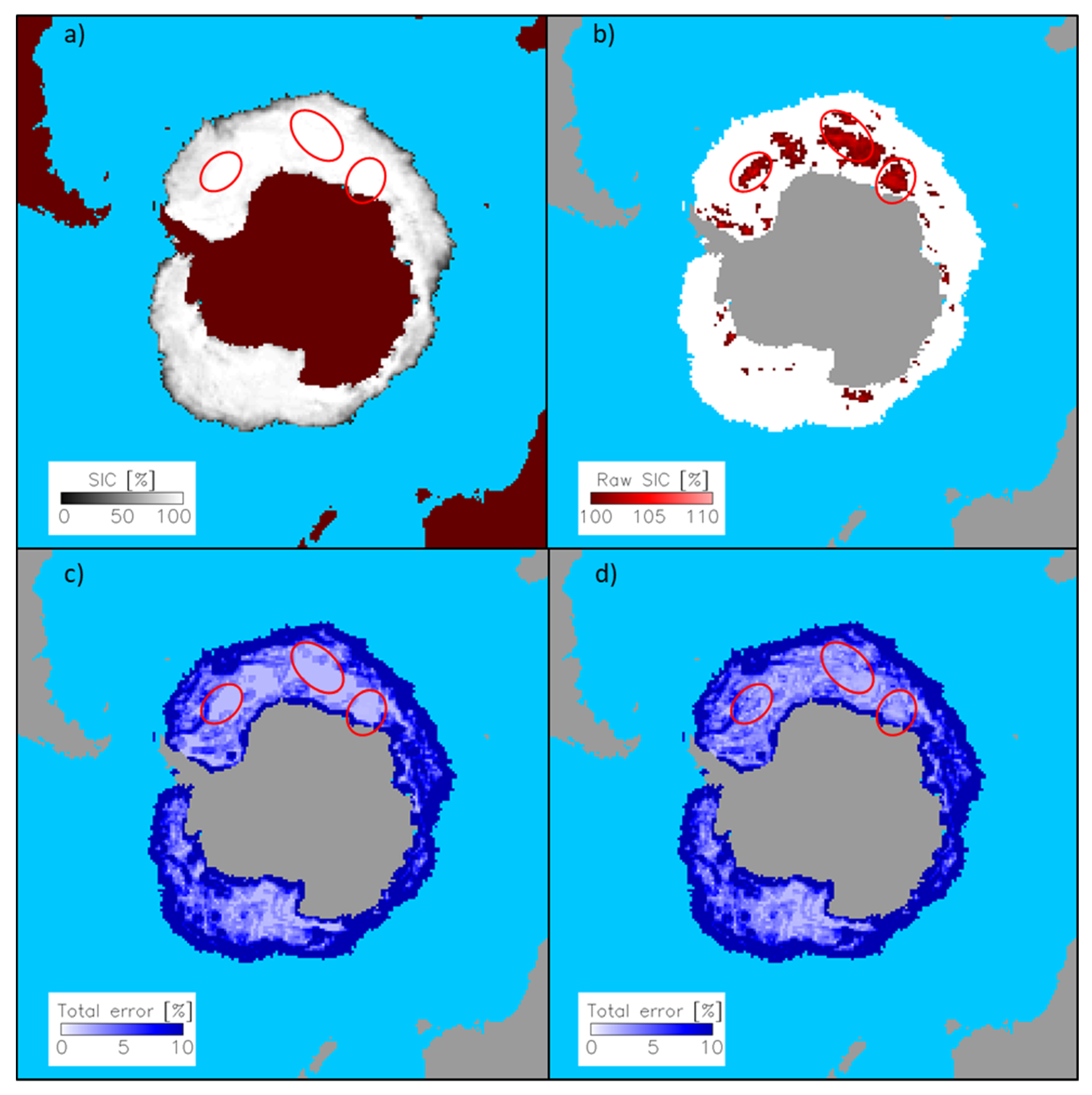
For regions of 100% (and 0%) sea-ice concentration, εrepresentativity is zero, and consequently, εtotal = εalgorithm. This also applies to those grid cells where non-truncated SIC values are larger than 100% (smaller than 0%). With that, neither the representativity nor the total error are smooth functions of the actually retrieved sea-ice concentration, and it is not possible to use these in the analysis planned (see Section 3). Therefore, in a first step, I computed εrepresentativity and εtotal also for grid cells with non-truncated SIC > 100%. For this, following [9,13], I first identified the minimum and maximum values of the non-truncated SIC for every 3 × 3 grid-cell box centered at the grid cell in question and computed εrepresentativity using Equation (1). Subsequently, applying Equation (2), I derived εtotal using εrepresentativity just computed and taking εalgorithm from the respective data file. Finally, I replaced the original total error value with this new value. Figure 1 and Figure 2 show examples of the truncated SIC, the non-truncated SIC, the original total error and the corrected total error for one sample day in the Northern and Southern Hemispheres, respectively. Regions with pronounced fractions of SIC > 100% are highlighted.

3. Methods

The above-mentioned ESA-CCI SST gap-filled Level-4 product [19] provides estimates of the total error for which computation of the different characteristics and spatiotemporal scales of the error components of the Level-2 and -3 products—random or uncorrelated, local-scale correlated and large-scale correlated—were taken into account (see [29]). The spatiotemporal scales at which the OSISAF–ESA-CCI sea-ice concentration error components (see Equation (2)) vary or are correlated is not yet well known. Similar to the SST product, there is one random, presumably uncorrelated, component, εalgorithm, and there are two larger-scale correlated components. One is εrepresentativity, which, by construction, is correlated regionally at the spatiotemporal scales of SIC gradients being large enough for this error contribution to exhibit a notable value. The second is the observational error or bias, which occurs due to actual sea-ice (surface) conditions not matching the conditions represented by the tie points used or due to weather effects.
One way to obtain information about the scales at which the errors of a Level-4 product are correlated is to estimate their correlation length scales, as suggested, e.g., by Bellprat et al. [30], or as carried out in the form of computations of the e-folding temporal and spatial scales in sea-ice data from numerical modeling and reanalyses [20,31]. In this study, I investigate the spatial correlation length scales of the observational error or bias for near-100% SIC values, called SIC error henceforth, and the total error εtotal (see Equation (2)). While εtotal is available from the OSISAF–ESA-CCI datasets for every grid cell (see Section 2), the SIC error is not. Its derivation would require daily pan-Arctic and -Antarctic, highly accurate, independent, i.e., other than from satellite microwave radiometry, SIC estimates. These are not available from other satellite remote sensing observations. I could have used sea-ice concentration from a numerical model output. However, this might have introduced additional biases and/or different spatiotemporal scales. In order to avoid this, I approximated the SIC error near 100% by subtracting 100% from the non-truncated SIC values for all grid cells with at least 90% SIC. The residual I consider the SIC error near 100%. I used 90% instead of a higher SIC value, i.e., 95%, in order to be able to carry out the analysis also during the beginning of the melt season known for larger SIC errors when compared to winter. Using 90% also fits with the idea to—at least theoretically—allow a symmetric SIC error distribution around 100% in light of the observation that non-truncated SIC values can be as high as 110%.
The first step is to compute so-called one-point correlation maps (see, e.g., [20]). For every grid cell and every day of one year, I compute the cross-correlation rij between the 31-day error time series and all error time series of the same length and period within a radius of 1000 km around this grid cell (Equation (3)).
r i j = t = 1 31 ( ε 0 ( t ) ε 0 ) ( ε i j ( t ) ε i j ) t = 1 31 ( ε 0 ( t ) ε 0 ) 2 t = 1 31 ( ε i j ( t ) ε i j ) 2
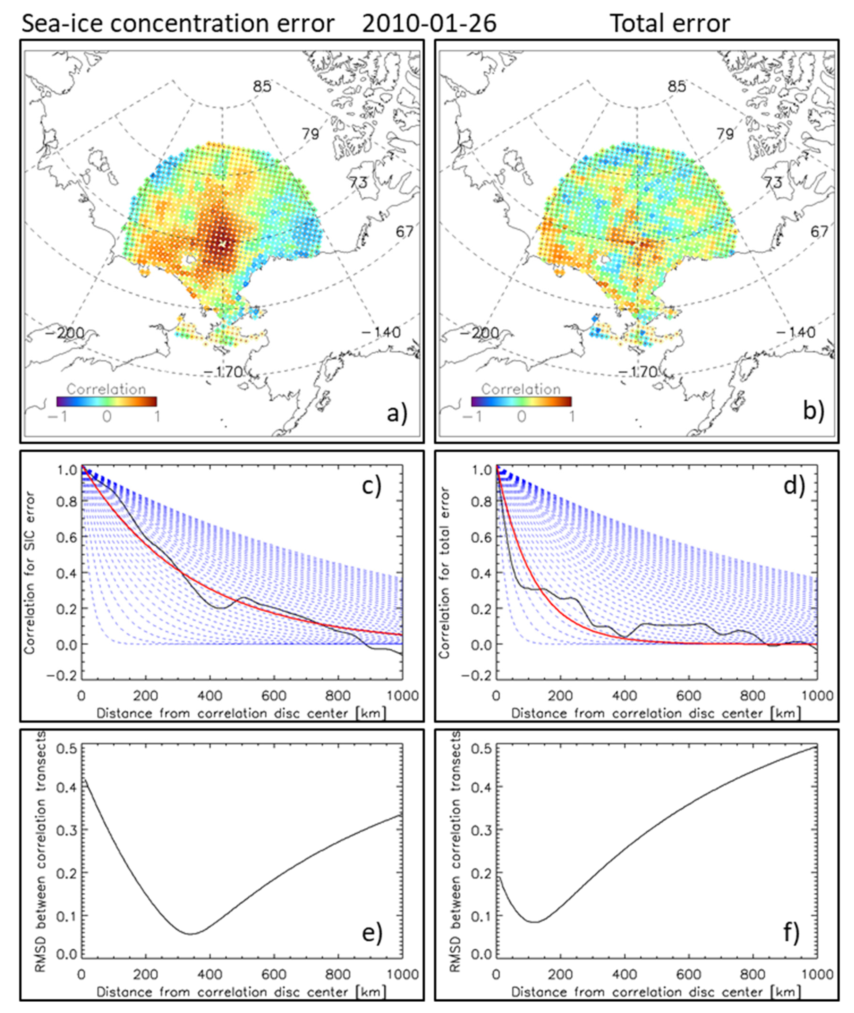
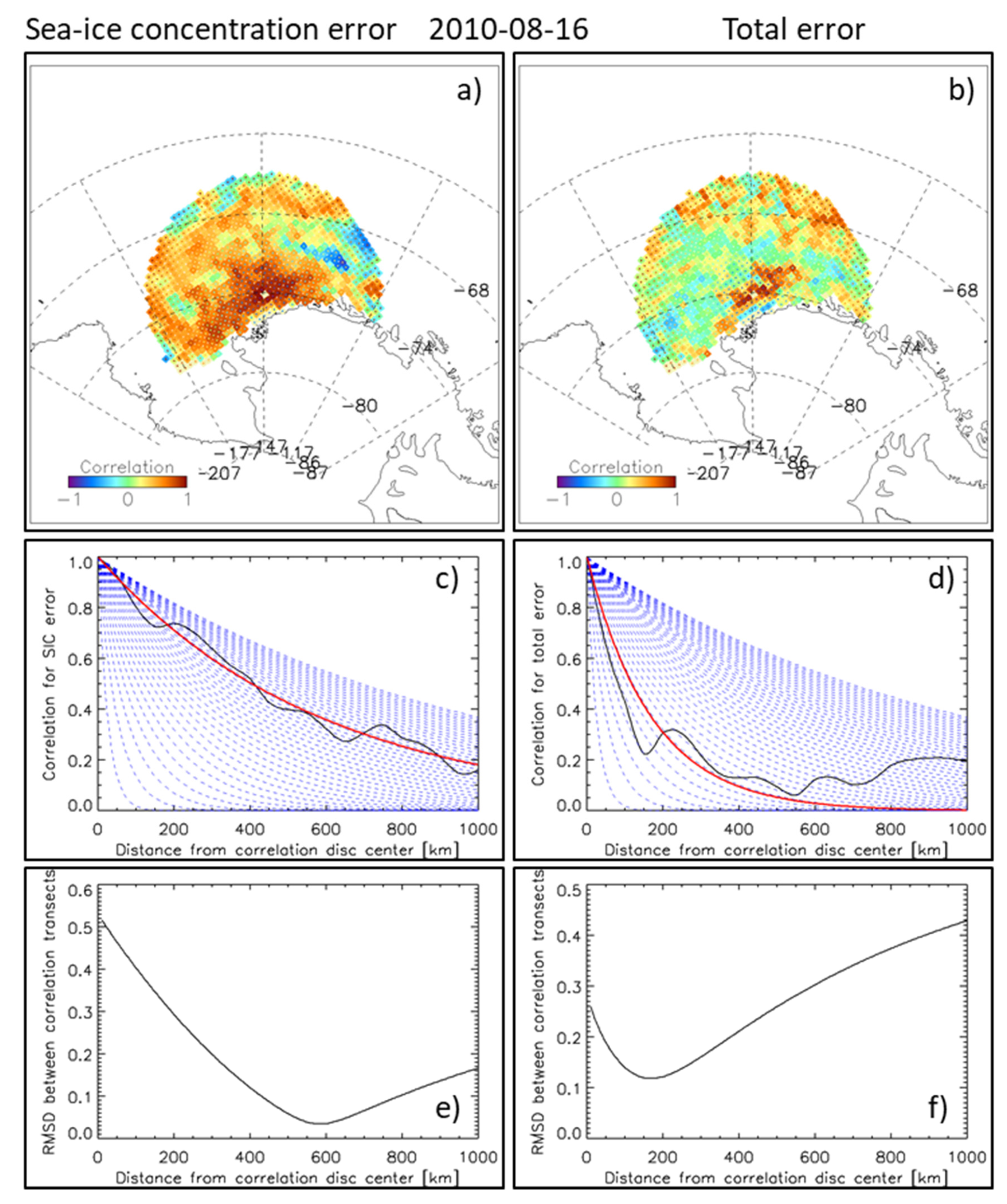
where t is the time in days, ε 0 ( t ) is the error at the center grid cell at day t, ε 0 is the error at the center grid cell averaged over the 31 days, ε i j ( t ) is the error within the 1000 km radius disc at i-th (x-coordinate) and j-th (y-coordinate) grid cells at day t and ε i j is its respective temporal average over the 31 days. With that, for every grid cell, the correlation analysis involves a stack of 31 discs of 1000 km radius. The 31-day period centers at the day of interest, i.e., for 16 January, I use the period 1 January through 31 January. The minimum fraction of the net, i.e., without land contribution, disc area covered by grid cells with at least 90% SIC needs to be one quarter in order to be used in the computation of the correlation. I use the land cover data provided with the three SIC products. The minimum number of days with a valid SIC value, i.e., greater than or equal to 90%, needs to be 16 for each time series. The spatial distribution of the correlation coefficients rij across the 1000 km radius disc, termed “correlation disc” henceforth, I save for every day and every grid cell with a valid SIC value. Examples of such correlation discs for SIC error and total error are shown in Figure 3a,b and Figure 4a,b.
I estimate the correlation length scale L as follows. First, for every correlation disc, I derive the average correlation coefficient r i j for rings concentric to the center grid cell. The width of the rings is set to 5 km and is hence smaller than the grid resolution of the used products: 25 km or 50 km (see Table 1). Any transect from the center grid cell to the edge of the disc now describes the change (decay) of the correlation as a function of distance X to the center grid cell (see also, e.g., [20]); X runs from 5 km to 1000 km in steps of 5 km.
Subsequently, I compute a suite of n = 196 hypothetical exponential functions describing the decay of the hypothetical correlation as a function of distance X and a hypothetical correlation length scale (in kilometers) L h y p o :
r h y p o = e x p ( X L h y p o ) ,   L h y p o { 20 ,   25 ,   30 ,   ,   990 ,   995 ,   1000 }
The result is a set of n = 196 decaying hypothetical exponential functions of the correlation along the transect given by the distance vector X. Examples of such sets are shown in Figure 3c,d and Figure 4c,d. Finally, I compute the root-mean-squared differences (RMSD) between the actually observed and this set of hypothetical correlation functions:
R M S D k = 1 n = k = 1 n ( r i j r h y p o ) 2 n ,   L = L h y p o ( k )   for   R M S D k = M I N ( R M S D k = 1 n )
I derive the final correlation length scale L as that value of L h y p o which results in the minimum RMSD value when used in Equations (4) and (5) (see Figure 3e,f and Figure 4e,f). If two hypothetical functions provide the same minimum RMSD value, I take the average of both L h y p o values as L. This way, I compute the correlation length scale for every grid cell with a useful correlation disc providing daily pan-Arctic/-Antarctic maps of the correlation length-scale distribution separately for the SIC error and the total error (see Section 4). These maps are stored together with the associated minimum RMSD value in netCDF file format available at https://www.cen.uni-hamburg.de/icdc (last accessed on 2 November 2021).
Common to both Figure 3 and Figure 4 is that the correlation for the SIC error (Figure 3a and Figure 4a) tends to show larger spatial coherence around the center of the disc, i.e., the location with which the correlation is computed, than the correlation shown for the total error (Figure 3b and Figure 4b). Consequently, the mean correlation decreases faster away from the disc’s center for the total error (Figure 3d and Figure 4d) than for the SIC error (Figure 3c and Figure 4c). This results in a larger correlation length scale for the SIC error (Figure 3e and Figure 4e) than for the total error (Figure 3f and Figure 4f), as illustrated by the location of the minimum RMSD. I get back to this observation in Section 4.

4. Results

Figure 5 illustrates how, for a sample region in the Northern Hemisphere north of the Canadian Arctic Archipelago, the correlation analysis distributes over time, showing correlation discs and RMSD profiles. For this region, one can investigate almost the full seasonal cycle because the sea-ice concentration is larger than 90% over a large enough area even during summer. This is not the case for first-year ice-covered regions. Hence, the spatiotemporal coverage with correlation length-scale data is most complete during the freezing season but exhibits gaps during summer melt and towards the ice edge.
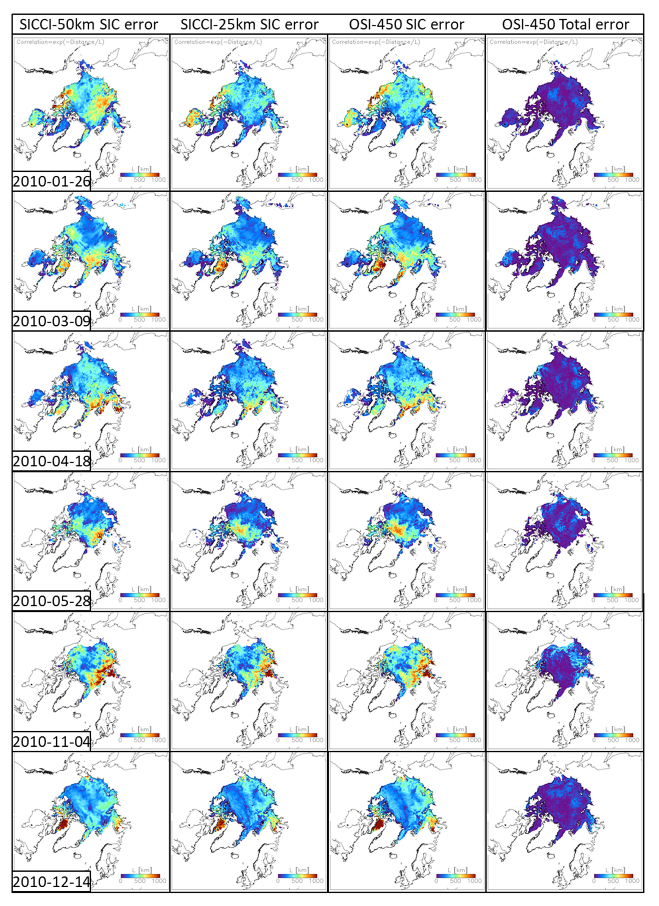
Figure 5 reveals also that one needs to consider the correlation disc examples shown in Figure 3 as a snapshot in time because the spatial distribution and coherence of the correlation values around the disc’s center varies with time and so does the correlation length scale. I get back to the variation in the spatial distribution of the correlation values in Section 5.1. Of the sample dates shown, it is comparably small for 16 August: ~150 km and 14 December: ~200 km, and largest for 28 May and 9 March: ~470 km. Figure 6 illustrates how error correlation length scales distribute across the Arctic Ocean.
Maps in the leftmost column show SIC error correlation length scales for SICCI-50km, i.e., the product whose results are also shown in Figure 3 and Figure 5. These maps reveal the two dates with the largest correlation length scales north of the Canadian Arctic Archipelago discussed above (Figure 5) are part of comparably large areas exhibiting SIC error correlation length scales between ~400 km and ~800 km extending from north of Svalbard and Franz-Josef-Land into the Beaufort Sea. The remaining regions exhibit considerably smaller SIC error correlation length scales at 2010-03-09 and 2010-05-28, except Baffin Bay on 2010-03-09. For 2010-12-14, the respective SIC error correlation length-scale map reveals that the conditions illustrated in Figure 5 belong to an area exhibiting SIC error correlation length scales below ~300 km fringing the Canadian Arctic Archipelago. Hence, the values exemplified in Figure 5 belong to larger-scale patterns of the correlation length scale.
The spatial distribution of regions with small or large SIC error correlation length scales is, at first glance, quite similar between the three products shown. Both patterns and absolute values are similar, particularly for SICCI-25km and OSI-450 in the Northern Hemisphere (Figure 6, compare middle left and middle right columns) but also in the Southern Hemisphere (Figure 7). In the Northern Hemisphere, the largest difference between SICCI-50km on the one hand and SICCI-25km and OSI-450 on the other hand occurs on 2010-05-28 when SICCI-50km reveals the largest SIC error correlation length scales north of Barents Sea, while the other two products reveal these north of the Canadian Arctic Archipelago. Another less pronounced example is 2010-12-14, when SICCI-50km shows larger SIC error correlation length scales north of Fram Strait than the other two products. In the Southern Hemisphere, inter-product differences are less pronounced and less coherent between the products.
Examples of the total error correlation length scales I show for OSI-450 in the rightmost columns of Figure 6 and Figure 7. These length scales rarely exceed 300 km and, with that, are mostly substantially smaller than the respective SIC error correlation length scales. This is in line with the panels shown in Figure 3 and Figure 4 in their right columns. The correlation discs suggest less spatial coherence and the steeper decay of the correlation with distance to the disc’s center results in a smaller correlation length scale. I find little coherence between locations with elevated total error correlation length scales and locations with elevated SIC error correlation length scales in both hemispheres (compare middle right and rightmost columns in Figure 6 and Figure 7). This is in line with my expectations (see Section 5.2).

5. Discussion

5.1. Methodological Aspects

I tested smaller (500 km) and larger (2000 km) correlation disc radii. Using 500 km, I often failed to arrive at a minimum RMSD value (Equation (5)). This is not surprising given the results shown in Figure 6 and Figure 7, suggesting that particularly the SIC error correlation length scales are often as large as 700 km or more. Using 2000 km, I obtained a smaller spatiotemporal coverage because of the methodological requirements (see Section 2), and I was facing a larger number of data gaps within the correlation disc area. In addition, the computation time increased substantially. Another argument against using 2000 km is the fact that I average the correlation values on concentric rings around the correlation disc’s center. The larger these rings become, the larger gets the net area over which I average the correlation values, and the more uncertain is my assumption of a radially symmetric decay of the correlation away from the disc’s center. Therefore, my choice of 1000 km, which is already a compromise.
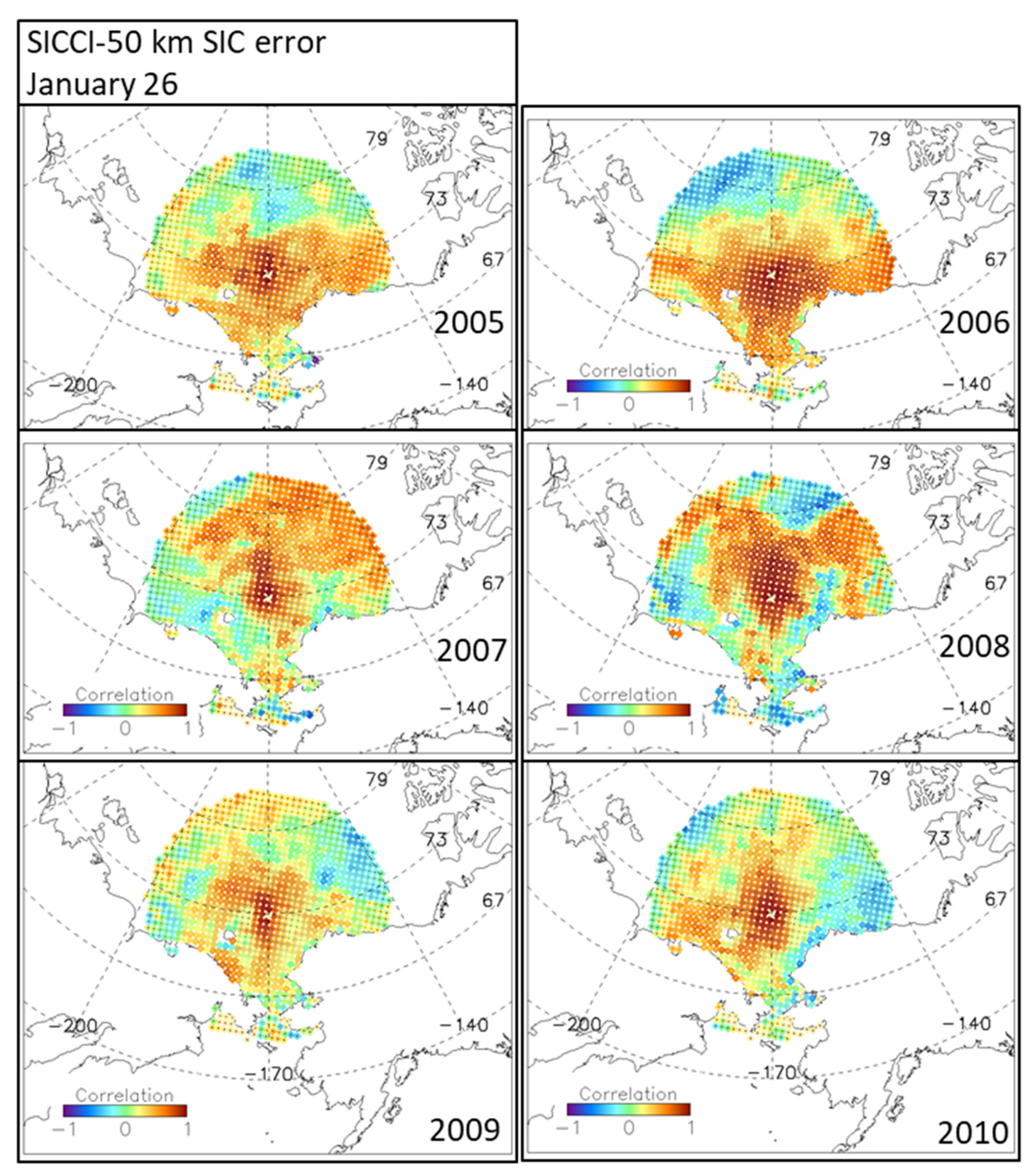
The assumption of a radially symmetric decay of the correlation away from the disc’s center deserves further discussion. On the one hand, with my approach, I am following previous work investigating correlation length scales in the Arctic Ocean [20,31], both being based on computing one-point cross-correlation maps and fitting a circle to the region within which the correlation exceeded 1/e to obtain the e-folding length scale. On the other hand, examples of the correlation discs shown in Figure 3, Figure 4 and Figure 5 (see Section 3 and Section 4) and Figure 8 and Figure 9 (see below) suggest that the assumption of circular symmetry might not be justified at every location. For the example north of the Bering Strait (Figure 3a,b, Figure 8 and Figure 9), the assumption of circular symmetry appears to apply well. In contrast, the case shown for the Amundsen Sea, Southern Ocean (Figure 4a,b), suggests that the circular symmetry is disturbed near the coast and that, instead of using circular rings to compute r i j (see Section 3), elliptical rings would be more appropriate. The same is suggested by Figure 5, which can be considered an extreme case, however, because the center of the correlation disc is located right off the coast. Alternatively, instead of computing r i j one could derive the correlation length scale L for individual profiles of r i j taken as vectors pointing outwards from the disc’s center. While this would provide a better representation of the spatial variability of L in accordance with the distribution of the correlation across the disc, one would need to find an appropriate way to express this variability and the most probable value of L at that grid cell for which this particular correlation disc is computed.
The distributions of the correlation obtained for the total error in Figure 3b, Figure 4b and Figure 9b appear to be more random and are likely less influenced by the choice of averaging geometry used to compute r i j . Additionally, the faster decay of the correlation values away from the disc’s center (compare Figure 8 and Figure 9) supports the notion that any violation in circular symmetry likely has a smaller impact than for the SIC error correlation. This also applies to extreme locations of the disc’s center such as those shown in Figure 5; only during summer and fall do gradients in εtotal cause a correlation distribution not supporting circular symmetry (not shown).
The conclusions from these considerations are that my results should be interpreted carefully in regions close to the coast, as well as close to the edge of high-concentration (>90%) ice. This applies in particular to L obtained for the SIC error, or in general large SIC error correlation length scales, while L values obtained for εtotal are generally smaller, allowing a larger fraction of reliable values also near coasts and the edge of high-concentration ice.
I note that not all of the obtained functions describing the evolution of r i j away from the correlation disc’s center are as smooth as those shown in Figure 3c,d and Figure 4c,d (black solid line). Consequently, the fit between r h y p o and the line of r i j is at times not overly good, resulting in a comparably large minimum RMSD value used to derive L (see Equation (5)). In order to provide users with some sort of a measure of the quality of L, the data set includes maps of the respective minimum RMSD value for every day for both the SIC error and the total error correlation length scales.
The total error comprises contributions of εalgorithm, i.e., brightness temperature noise and tie point variability, and εrepresentativity, i.e., contributions from the averaging and gridding of the SIC computed at the footprint scale into the EASE grid (see Section 2, Equation (2)). In this study, I did not investigate correlations of εalgorithm in depth. The spatiotemporal variation of εalgorithm is very small, and it is highly correlated across the high-concentration pack ice considered here. Consequently, correlation values decay very slowly away from the correlation disc’s center, resulting in correlation length scales (not shown) beyond what can be retrieved reasonably using my approach or using the one of [20].
The total error correlation length scales shown in this paper can be dominated by contributions of εrepresentativity and hence strongly depend on the spatial SIC gradient (see Equation (1) and [13]). With that, my computations of these length scales are influenced by the different spatial scales involved in the derivation of εrepresentativity. The 3 × 3 grid-cell neighborhood used is of size 75 km × 75 km for SICCI-25km and OSI-450 and 150 km × 150 km for SICCI-50km. This influences both the magnitude and the distribution of εrepresentativity within a certain area, which can have an impact on the total error correlation length scales obtained.
SIC estimates of all swath-based satellite observations within one day are averaged into the Level-4 OSISAF–ESA-CCI SIC products used here. While εrepresentativity provides information about the error contribution due to the spatial averaging, it lacks information about the potential error contribution due the temporal averaging. Given the large grid and footprint sizes used (Table 1) and the typically, at that scale, slowly varying sea-ice concentration, inclusion of the temporal component seems to be not required here. What I could have done, though, is to compute temporal auto-correlations of the 31-day SIC error and total error time series forward in time to obtain information about the time scale (or the persistence) of variation of these time series (see also [20]). This is planned for a forthcoming study.

5.2. Interpretation of the Results

Particularly high positive correlations one can expect to find in the case of homogeneous large-scale changes in the surface emissivity of the sea ice being in phase with those at the correlation disc’s center. One typical scenario for this could be weather-influence-induced changes in the snow and sea-ice surface properties. These typically cover synoptic spatial scales, i.e., of the order of several hundreds of kilometers and may occur a few times during the 31-day period. Such changes often cause SIC variations by a few percent and therefore can result in a widespread decrease in SIC below 100% (negative SIC error) or increase above 100% (positive SIC error) (e.g., [9]). By utilizing the non-truncated (or raw) SIC data of the OSISAF–ESA-CCI products, I can consider changes in both these directions. Such weather-induced changes occur frequently and year-round over Southern Ocean sea ice even up to the coast and repeatedly over Arctic Ocean sea ice facing the northern North Atlantic and, during fall, also the interior Arctic Ocean. A number of the regions showing larger, i.e., >500 km, SIC error correlation length scales in Figure 6 and Figure 7 (left three columns) could potentially be attributed to such weather-induced changes. Another typical scenario could be onset of melt/commencement of freeze-up. Both processes also change snow and sea-ice surface properties on larger spatial scales depending on the north- or southward progressing increase or decrease in surface solar radiation. These processes can also trigger large-scale changes in the surface emissivity and hence sea-ice concentration that can result in SIC error variations over time in phase between the disc’s center and the surrounding grid cells, resulting in a high correlation. The consequence here could also be a comparably large SIC error correlation length scale.
However, it is not the magnitude of the correlation that determines the SIC error correlation length scale but the distance within which the correlation, on average, decreases away from the correlation disc’s center. If SIC error time series are correlated well within a few grid cells’ neighborhood to the correlation disc’s center and then become less correlated or even show an anti-correlation, then correlation length scales can be quite small despite a very high correlation near the disc’s center. This is exemplified by the SIC error in Figure 3a and Figure 5b. It is therefore important to consider spatiotemporal scales and the frequencies with which processes (e.g., surface melt, re-freeze, flooding) and changes in relevant geophysical parameters (e.g., snow, ice type) determining the sea-ice surface emissivity and hence sea-ice concentration and SIC error occur.
I stated above that a number of the regions exhibiting large SIC error correlation length scales in Figure 6 and Figure 7 could be associated with a frequently occurring weather influence. However, such large SIC error correlation length scales could also be a manifestation of a rather stable SIC error varying little but still in phase over a large region within the 31-day period considered. Such a region would indicate stable sea-ice (surface) conditions. In contrast to that, regions subject to weather-induced changes might show a rather small SIC error correlation length scale in case sea-ice surface conditions within the correlation disc do not vary in phase with conditions at the disc’s center. This appears to be quite likely because, over the course of a month, depending on the location, sea-ice surface conditions at the disc’s center would only vary in phase with surrounding grid cells’ conditions if the weather influence stays the same. This would require, e.g., the cyclone to always move along the same track, snowfall or freezing rain to always cover the same regions, and spatial air temperature variations to always be similar in terms of their impact on melt/re-freeze. I do not exclude that such cases could occur temporarily, e.g., for a duration of one/two months, and in certain regions, e.g., the northern Amundsen Sea, due to the stability of certain atmospheric circulation regimes, e.g., the Amundsen Sea Low. I would suggest, however, these are less common. Hence, in summary, I suggest regions subject to a weather influence on sea-ice surface conditions can exhibit small, as well as large, SIC error correlation length scales, depending on the frequency of the events and depending on the nature of the sea-ice surface condition changes (short-lived or longer duration) encountered (e.g., [32,33]). This suggestion is supported by the quite variable SIC error correlation length scales shown for the area stretching from the Bellingshausen over the Amundsen into the Ross Sea in Figure 7 (left columns, 2010-05-28 until 2010-11-04), a region known for frequent and variable weather influence.
Sub-grid-scale openings in the sea-ice cover such as leads and polynyas reduce the SIC derived below 100%. For thin ice, passive microwave SIC algorithms are also known to provide too low SIC values (e.g., [8]). Therefore, one can expect that regions subject to such openings and/or notable fractions of thin ice exhibit SIC < 100%; these regions would rarely exhibit SIC > 100%. This has consequences for the interpretation of my results. Regions within the correlation disc that experience frequent deformation (opening and closing) of the sea-ice cover potentially exhibit SIC variations of a few percent, translating into mostly negative SIC errors of a few percent, which are correlated in various ways to the SIC error at the disc’s center, depending on the deformation there. In the Southern Ocean, such deformation events are mostly associated with the above-mentioned cyclonic activity. These therefore add to the weather influence on the SIC and hence SIC error, supporting small SIC error correlation length scales, especially in the above-mentioned area but also in general in a several 100 kilometers wide belt inside the ice edge. In the Arctic Ocean, during winter, when the entire basin is ice covered, deformation events might be less frequent but could affect large regions such as the entire Beaufort Sea. SIC variations due to lead and thin ice formation associated with deformation events could be responsible for the comparably large SIC error correlation length scales in the Beaufort Sea (e.g., in Figure 6, left three columns, 2010-01-26 and 2010-03-09). According to Willmes and Heinemann [34] and Reiser et al. [35], lead frequencies in this region were higher than in the central Arctic in winter 2010.
For the total error, correlations tend to decrease faster away from the correlation disc’s center (Figure 3b and Figure 4b), resulting in considerably smaller correlation length scales than observed for the SIC error (Figure 6 and Figure 7, rightmost column). I explain this with the observation that in the high-concentration areas (SIC > 90%) considered in this study, the total error εtotal is mainly determined by εalgorithm and less by εrepresentativity (see Section 2). The latter gains influence in case enhanced SIC gradients occur, e.g., in regions subject to leads, causing a reduction in the SIC, and in regions subject to other small-scale (3 × 3 grid cells, see Equation (1)) SIC variations on both sides of 100%, retrieval noise and noise, due to sea-ice surface emissivity variations induced by weather or melt onset. The SIC variations need to be large enough to cause a notable contribution to εtotal via εrepresentativity (see Section 2). Figure 1d and Figure 2d reveal variations in εtotal of the order of a few percent on top of εalgorithm, which, during winter, takes values of 2–3%. With that, variations in εtotal are small compared to the variations in the SIC error, and consequently, correlation values tend to be smaller on average. The spatial distribution of the correlation coefficient obtained for total error time series within the correlation discs often appears to be considerably more arbitrary than for the SIC error time series (see, e.g., Figure 3b). Therefore, the average correlation often drops rather quickly away from the disc’s center, resulting in the small total error correlation length scales observed.
The time series of correlation length scales and respective minimum RMSD values in the year 2010 shown in Figure 10 for an arbitrarily selected region in the central Arctic Ocean reveal several important additional aspects. Time series of the correlation length scales of both SIC error and total error are very similar for OSI-450 and SICCI-25km. This applies to the temporal variation and the magnitude of the values before the data gap in summer; after summer, variations are similar, but magnitudes are larger for OSI-450. While variation and magnitudes are also similar for SICCI-50km, this product shows substantially larger, compared to the other two products, total error correlation length scales in the weeks prior to the summer gap (after day of the year 135, i.e., mid-May). Investigation of the respective correlation discs reveals averaged correlation values (see Section 3) larger than 0.5 for the entire correlation disc (not shown). This increase in total error correlation length scale prior to the summer gap also occurs in other years of the period 2003–2010 (Figure 11b). I note, however, SIC error correlation length scales increase considerably during the last week before the summer gap, as do the total error correlation length scales, for all three products (Figure 10). This increase just prior to the summer gap, which is due to SIC values dropping below 90%, is possibly related to a combination of several factors. One such factor is increased SIC noise due to melt causing an elevated number of grid cells with >100% SIC (see [11]) along with first openings in the ice cover not freezing over anymore and melt ponds on the sea ice. Another factor could be the reduction in the high-concentration area mentioned in Section 5.1 as one potential limitation for the validity of one aspect of my derivation of L.
Why SICCI-50km total error correlation length scales respond to the first signs of melt onset during mid-May so strongly requires further investigation. It might be related to the way εtotal is derived in combination with the coarse grid resolution. First, as briefly mentioned in Section 5.1, over high-concentration ice, variations in εtotal are determined by variations in εrepresentativity. The latter can be expected to be less variable for SICCI-50km compared to SICCI-25km because of the coarser grid resolution. For a 150 km × 150 km large area, one has 6 × 6 = 36 grid cells for SICCI-25km and 3 × 3 = 9 grid cells for SICCI-50km. This results in 4 × 4 = 16 individual values of εrepresentativity for SICCI-25km and just one value of εrepresentativity SICCI-50km. Second, as summer melt approaches, SIC gradients caused by different ice types and snow surface properties are blurred by the effects of surface melt. While these effects could be quite heterogeneous [11], I hypothesize that the smoothing induced at a grid resolution of 50 km reduces SIC variability at the scale relevant for the computation of εrepresentativity down towards a level causing εrepresentativity to vary as little as εalgorithm (see also my comment with respect to εalgorithm in Section 5.1).
Finally, despite the limitation to the arbitrarily selected year 2010, I provide a glimpse into other years. In Figure 8 and Figure 9, I demonstrate by means of the location used in Figure 3 that the one-point correlation maps forming the foundation for the estimation of the correlation length scales can be reproduced every year (shown are years 2005 to 2010), exhibiting similar spatial distributions of the correlation. In Figure 11, I show for those years of the AMSR-E observation period where a full year of observations was possible, i.e., 2003 through 2010, the inter-annual variation of the SIC error (Figure 11a) and total error (Figure 11b) correlation length-scale time series for the region near Wrangell Island used in Figure 10. For that region, taking a SIC error correlation length scale between 200 km and 400 km appears to be a reasonable choice during most of winter. Typical correlation length scales obtained for the total error are considerably smaller, ranging between 50 km and 200 km between January and April and a little higher during late fall/early winter. Inter-annual variations in onset, length and particularly end of the summer period appear to influence the total error correlation length scales in late fall/early winter (Figure 11b). The variations in onset and end of the summer period suggest varying periods during which, e.g., a constant value of L can be used to characterize the correlation of the errors. While I observe considerable variations in the SIC error correlation length scales across the years, together with an indication of a negative trend across the winter (Figure 11a), it is beyond the scope of this paper to investigate this in more detail. Changes in the weather-induced sea-ice and snow surface properties appear to be the most promising candidate for explanations here.
To fully understand and interpret the spatial distribution of the correlations and the correlation length scales shown and use this information for further improvement of, e.g., the SIC retrieval or estimation of the total error, requires taking additional information into account. Information I suggest to include are:
  • The ice type (new ice, first-year ice, multi-year ice) because changes in surface emissivity by weather influence or the seasonal cycle are a function of the ice type. The rather sharp gradient in the SIC error correlation length scale across the central Arctic Ocean I find for all three products (Figure 6, 2010-05-28, left three columns) appears to point in this direction.
  • The age of the seasonal sea ice because the surface emissivity changes most during the first days/weeks of its formation in response to changes in sea-ice surface properties such as salinity and temperature. The comparably well-defined area with (high) positive correlations near the correlation disc’s center paired with negative correlations north of Alaska and towards the West (Figure 3a) appears to point towards the importance of this parameter.
  • The surface temperature and/or snow accumulation history (melt/freeze cycles, snowfall events) because sea-ice surface emissivity is, to a large extent, determined by the properties of the overlying snow (snow metamorphism) and interactions at the snow–ice interface (flooding, formation of meteoric ice). The importance of this information is evident in Figure 4a by a quite substantial variation in the SIC error time-series correlation across the correlation disc and in Figure 7 (left three columns) by the large spatial variability of the SIC error correlation length scale over basically the entire high-concentration sea-ice cover.
  • Finally, the lead frequency because reduction in the SIC below 100% by sub-grid-scale openings and thin ice areas influences the SIC error time series and its spatial correlation in regions with high sea-ice dynamics and is suggested to result in comparably large SIC error correlation length scales as evidenced in Figure 6, 2010-01-26 and 2010-03-09 in the Beaufort Sea.

6. Conclusions

This manuscript presents the results of a first attempt to provide information about SIC error and total error correlation length scales derived from satellite observations based on OSISAF–ESA-CCI SICCI-25km, SICCI-50km and OSI-450 SIC products of the Arctic Ocean and the Southern Ocean in a post-processing step. Data of the total error are included in these products. This error comprises random components such as sensor and retrieval noise and locally-to-regionally correlated components describing the representativity error from the projection of the satellite observations into the used grid. In order to account for systematic errors related, e.g., to a mismatch between actual and retrieval-inherent ice conditions, I approximate the SIC error as the SIC anomaly with respect to 100% SIC for high-concentration (>90%) pack ice using the non-truncated OSISAF–ESA-CCI product SIC values; non-truncated means that naturally retrieved SIC values > 100% were preserved. Such errors originate from the sensitivity of the SIC retrieval to, e.g., ice type or weather influence and are likely correlated at a larger scale. I derive the correlation length scale L by fitting a set of hypothetical exponential functions to the function describing the decay of the mean correlation away from the center of one-point correlation maps of a 1000 km radius. These maps are derived separately for the SIC error and the total error by computing the cross-correlation of 31-day time series between the center grid cell and all other grid cells within the given radius.
I find the approach to work robustly and provide reasonable correlation length scales for the high-concentration pack ice for most of the freezing season and into spring. Correlation length scales are larger for the SIC error than for the total error. In 2010, typical values of total error L range between 50–100 km and 300–400 km. For the SIC error, L ranges mostly between 200–400 km and 500–700 km, also in 2010. I investigated time series of L for a region north of Wrangell Island, Arctic Ocean, using SICCI-50km for 2003–2010. These time series confirm the above-mentioned L values and reveal a similar temporal evolution of L in the years considered for both SIC error and total error.
The next generation of these SIC products could benefit from a computation of the total error, which takes into account the correlation of the different error contributions already during the retrieval process. Error contributions caused by small-scale variations in surface emissivity due to snow metamorphism might need to be treated in a different way than error contributions from the gridding process or caused by the algorithms’ sensitivity to larger-scale variations in ice type, thickness or weather influence that are yet difficult to quantify by means of the total error. Error correlation information as shown in this paper could assist in the quantification of the error margins of parameters such as sea-ice area and sea-ice extent derived from SIC products of the kind used here.

Funding

This research received no external funding. The publication contributes to the Cluster of Excellence ‘CLICCS–Climate, Climatic Change, and Society’ and to the Center for Earth System Research and Sustainability (CEN) of the University of Hamburg.

Institutional Review Board Statement

Not applicable.

Informed Consent Statement

Not applicable.

Data Availability Statement

OSI-450 data are available here: https://doi.org/10.15770/EUM_SAF_OSI_0008 (last accessed on 17 September 2021), SICCI-25km data are available here: https://doi.org/10.5285/f17f146a31b14dfd960cde0874236ee5 (last accessed on 17 September 2021), SICCI-50km data here: https://doi.org/10.5285/5f75fcb0c58740d99b07953797bc041e (last accessed on 17 September 2021). The data set of the correlation lengths scales for all three products for 2010 is available from ftp://cen.uni-hamburg.de/outgoing/icdc/SpatialSICerrorCorrelationLengthScales/ (last accessed on 2 November 2021), also accessible via https://www.cen.uni-hamburg.de/icdc (last accessed on 2 November 2021), or upon request from the author and will be published at https://www.fdr.uni-hamburg.de/ (last accessed on 2 November 2021).

Acknowledgments

I acknowledge the very helpful comments given by the two anonymous reviewers as well as the scientific editor. These helped to improve the manuscript substantially.

Conflicts of Interest

The author declares no conflict of interest.

References

  1. Meier, W.N.; Hovelsrud, G.K.; van Oort, B.E.H.; Key, J.R.; Kovacs, K.M.; Michel, C.; Haas, C.; Granskog, M.A.; Gerland, S.; Perovich, D.K.; et al. Arctic sea ice in transformation: A review of recent observed changes and impacts on biology and human activity. Rev. Geophys. 2014, 51, 185–217. [Google Scholar] [CrossRef]
  2. Parkinson, C.L.; DiGirolamo, N.E. New visualizations highlight new information on the contrasting Arctic and Antarctic sea-ice trends since the late 1970s. Remote Sens. Environ. 2016, 183, 198–204. [Google Scholar] [CrossRef] [Green Version]
  3. Stroeve, J.C.; Notz, D. Changing state of Arctic sea ice across all seasons. Environ. Res. Lett. 2018, 13, 103001. [Google Scholar] [CrossRef]
  4. Comiso, J.C.; Meier, W.N.; Gersten, R.A. Variability and trends in the Arctic Sea ice cover: Results from different techniques. J. Geophys. Res. Oceans 2017, 122, 6883–6900. [Google Scholar] [CrossRef]
  5. Comiso, J.C.; Gersten, R.A.; Stock, L.V.; Turner, J.; Perez, G.J.; Cho, K. Positive trends in the Antarctic sea ice cover and associated changes in surface temperature. J. Clim. 2017, 30, 2251–2267. [Google Scholar] [CrossRef] [PubMed] [Green Version]
  6. Parkinson, C.L. A 40-y record reveals gradual Antarctic sea ice increases followed by decreases at rates far exceeding the rates seen in the Arctic. Proc. Natl. Acad. Sci. USA 2019, 116, 14414–14423. [Google Scholar] [CrossRef] [PubMed] [Green Version]
  7. Meier, W.N.; Peng, G.; Scott, D.J.; Savoie, M.H. Verification of a new NOAA/NSIDC passive microwave sea-ice concentration climate record. Polar Res. 2014, 33, 21004. [Google Scholar] [CrossRef] [Green Version]
  8. Ivanova, N.; Pedersen, L.T.; Tonboe, R.T.; Kern, S.; Heygster, G.; Lavergne, T.; Sørensen, A.M.; Saldo, R.; Dybkjær, G.; Brucker, L.; et al. Inter-comparison and evaluation of sea ice algorithms: Towards further identification of challenges and optimal approach using passive microwave observations. Cryosphere 2015, 9, 1797–1817. [Google Scholar] [CrossRef] [Green Version]
  9. Lavergne, T.; Macdonald Sørensen, A.; Kern, S.; Tonboe, R.; Notz, D.; Aaboe, S.; Bell, L.; Dybkjær, G.; Eastwood, S.; Gabarro, C.; et al. Version 2 of the EUMETSAT OSI SAF and ESA-CCI sea-ice concentration climate data records. Cryosphere 2019, 13, 49–78. [Google Scholar] [CrossRef] [Green Version]
  10. Kern, S.; Lavergne, T.; Notz, D.; Pedersen, L.T.; Tonboe, R.T.; Saldo, R.; Sørensen, A.M. Satellite passive microwave sea-ice concentration data set intercomparison: Closed ice and ship-based observations. Cryosphere 2019, 13, 3261–3307. [Google Scholar] [CrossRef] [Green Version]
  11. Kern, S.; Lavergne, T.; Notz, D.; Pedersen, L.T.; Tonboe, R.T. Satellite passive microwave sea-ice concentration data set intercomparison for Arctic summer conditions. Cryosphere 2020, 14, 2469–2493. [Google Scholar] [CrossRef]
  12. Peng, G.; Meier, W.N.; Scott, D.; Savoie, M. A long-term and reproducible passive microwave sea ice concentration data record for climate studies and monitoring. Earth Syst. Sci. Data 2013, 5, 311–318. [Google Scholar] [CrossRef] [Green Version]
  13. Tonboe, R.T.; Eastwood, S.; Lavergne, T.; Sørensen, A.M.; Rathmann, N.; Dybkjær, G.; Pedersen, L.T.; Høyer, J.L.; Kern, S. The EUMETSAT sea ice concentration climate data record. Cryosphere 2016, 10, 2275–2290. [Google Scholar] [CrossRef] [Green Version]
  14. Burgard, C.; Notz, D.; Pedersen, L.T.; Tonboe, R.T. The Arctic Ocean observation operator for 6.9 GHz (ARC3O)—Part 2: Development and evaluation. Cryosphere 2020, 14, 2387–2407. [Google Scholar] [CrossRef]
  15. Tietsche, S.; Alonso-Balmaseda, M.; Rosnay, P.; Zuo, H.; Tian-Kunze, X.; Kaleschke, L. Thin Arctic sea ice in L-band observations and an ocean reanalysis. Cryosphere 2018, 12, 2051–2072. [Google Scholar] [CrossRef] [Green Version]
  16. Koldunov, N.V.; Köhl, A.; Serra, N.; Stammer, D. Sea ice assimilation into a coupled ocean-sea ice model using its adjoint. Cryosphere 2017, 11, 2265–2281. [Google Scholar] [CrossRef] [Green Version]
  17. Yang, Q.; Losch, M.; Losa, S.N.; Jung, T.; Nerger, L.; Lavergne, T. The challenge and benefit of using sea ice concentration satellite data products with uncertainty estimates in summer sea ice data assimilation. Cryosphere 2016, 10, 761–774. [Google Scholar] [CrossRef] [Green Version]
  18. Merchant, C.J.; Paul, F.; Popp, T.; Ablain, M.; Bontemps, S.; Defourny, P.; Hollmann, R.; Lavergne, T.; Laeng, A.; de Leeuw, G.; et al. Uncertainty information in climate data records from Earth observation. Earth Syst. Sci. Data 2017, 9, 511–527. [Google Scholar] [CrossRef] [Green Version]
  19. Merchant, C.J.; Embury, O.; Bulgin, C.E.; Block, T.; Corlett, G.K.; Fiedler, E.; Good, S.A.; Mittaz, J.; Rayner, N.A.; Berry, D.; et al. Satellite-based time-series of sea-surface temperature since 1981 for climate applications. Sci. Data 2019, 6, 223. [Google Scholar] [CrossRef] [Green Version]
  20. Ponsoni, L.; Massonnet, F.; Fichefet, T.; Chevallier, M.; Docquier, D. On the timescales and length scales of the Arctic sea ice thickness anomalies: A study based on 14 reanalyes. Cryosphere 2019, 13, 521–543. [Google Scholar] [CrossRef] [Green Version]
  21. Comiso, J.C. Characteristics of arctic winter sea ice from satellite multispectral microwave observations. J. Geophys. Res. 1986, 91, 975–994. [Google Scholar] [CrossRef]
  22. Comiso, J.C.; Nishio, F. Trends in the sea ice cover using enhanced and compatible AMSR-E, SSM/I, and SMMR data. J. Geophys. Res. 2008, 113, C02S07. [Google Scholar] [CrossRef]
  23. Comiso, J.C.; Cavalieri, D.J.; Parkinson, C.L.; Gloersen, P. Passive microwave algorithms for sea ice concentration: A comparison of two techniques. Remote Sens. Environ. 1997, 60, 357–384. [Google Scholar] [CrossRef]
  24. Comiso, J.C.; Cavalieri, D.J.; Markus, T. Sea ice concentration, ice temperature, and snow depth, using AMSR-E data. IEEE Trans. Geosci. Remote Sens. 2003, 41, 243–252. [Google Scholar] [CrossRef]
  25. Smith, D.M.; Barrett, E.C. Satellite Mapping and Monitoring of Sea Ice; Report. CB/RAE/9/2/4/2034/113/ARE, RSU; University of Bristol: Bristol, UK, 1994. [Google Scholar]
  26. Smith, D.M. Extraction of winter total sea ice concentration in the Greenland and Barents Seas from SSM/I data. Int. J. Remote Sens. 1996, 17, 2625–2646. [Google Scholar] [CrossRef]
  27. Brodzik, M.J.; Billingsley, B.; Haran, T.; Raup, B.; Savoie, M.H. EASE-Grid 2.0: Incremental but Significant Improvements for Earth-Gridded Data Sets. ISPRS Int. Geo-Inf. 2012, 1, 32–45. [Google Scholar] [CrossRef] [Green Version]
  28. Brodzik, M.J.; Billingsley, B.; Haran, T.; Raup, B.; Savoie, M.H. Correction: Brodzik, M.J. et al. EASE-Grid 2.0: Incremental but Significant Improvements for Earth-Gridded Data Sets. ISPRS Int. Geo-Inf. 2012, 1, 32–45, Erratum in 2014, 3, 1154–1156. [Google Scholar] [CrossRef] [Green Version]
  29. Donlon, C.J.; Martin, M.; Stark, J.; Roberts-Jones, J.; Fiedler, E.; Wimmer, W. The Operational Sea Surface Temperature and Sea Ice Analysis (OSTIA) system. Remote Sens. Environ. 2012, 116, 140–158. [Google Scholar] [CrossRef]
  30. Bellprat, O.; Massonnet, F.; Siegert, S.; Prodhomme, C.; Macias-Gomez, D.; Guemas, V.; Doblas-Reyes, F. Uncertainty propagation in observational references to climate model scales. Remote Sens. Environ. 2017, 203, 101–108. [Google Scholar] [CrossRef] [Green Version]
  31. Blanchard-Wrigglesworth, E.; Bitz, C.M. Characteristics of Arctic sea-ice thickness variability in GCMs. J. Clim. 2014, 27, 8244–8258. [Google Scholar] [CrossRef] [Green Version]
  32. Voss, S.; Heygster, G.; Ezraty, R. Improving sea ice type discrimination by the simultaneous use of SSM/I and scatterometer data. Polar Res. 2003, 22, 35–42. [Google Scholar] [CrossRef] [Green Version]
  33. Krumpen, T.; von Albedyll, L.; Goessling, H.F.; Hendricks, S.; Juhls, B.; Spreen, G.; Willmes, S.; Belter, H.J.; Dehtloff, K.; Haas, C.; et al. MOSAiC drift expedition from October 2019 to July 2020: Sea ice conditions from space and comparison with previous years. Cryosphere 2021, 15, 3897–3920. [Google Scholar] [CrossRef]
  34. Willmes, S.; Heinemann, G. Pan-Arctic lead detection from MODIS thermal infrared imagery. Ann. Glaciol. 2015, 56, 29–37. [Google Scholar] [CrossRef] [Green Version]
  35. Reiser, F.; Willmes, S.; Heinemann, G. A new algorithm for daily sea ice lead identification in the Arctic and Antarctic winter from thermal-infrared satellite imagery. Remote Sens. 2020, 12, 1957–1972. [Google Scholar] [CrossRef]
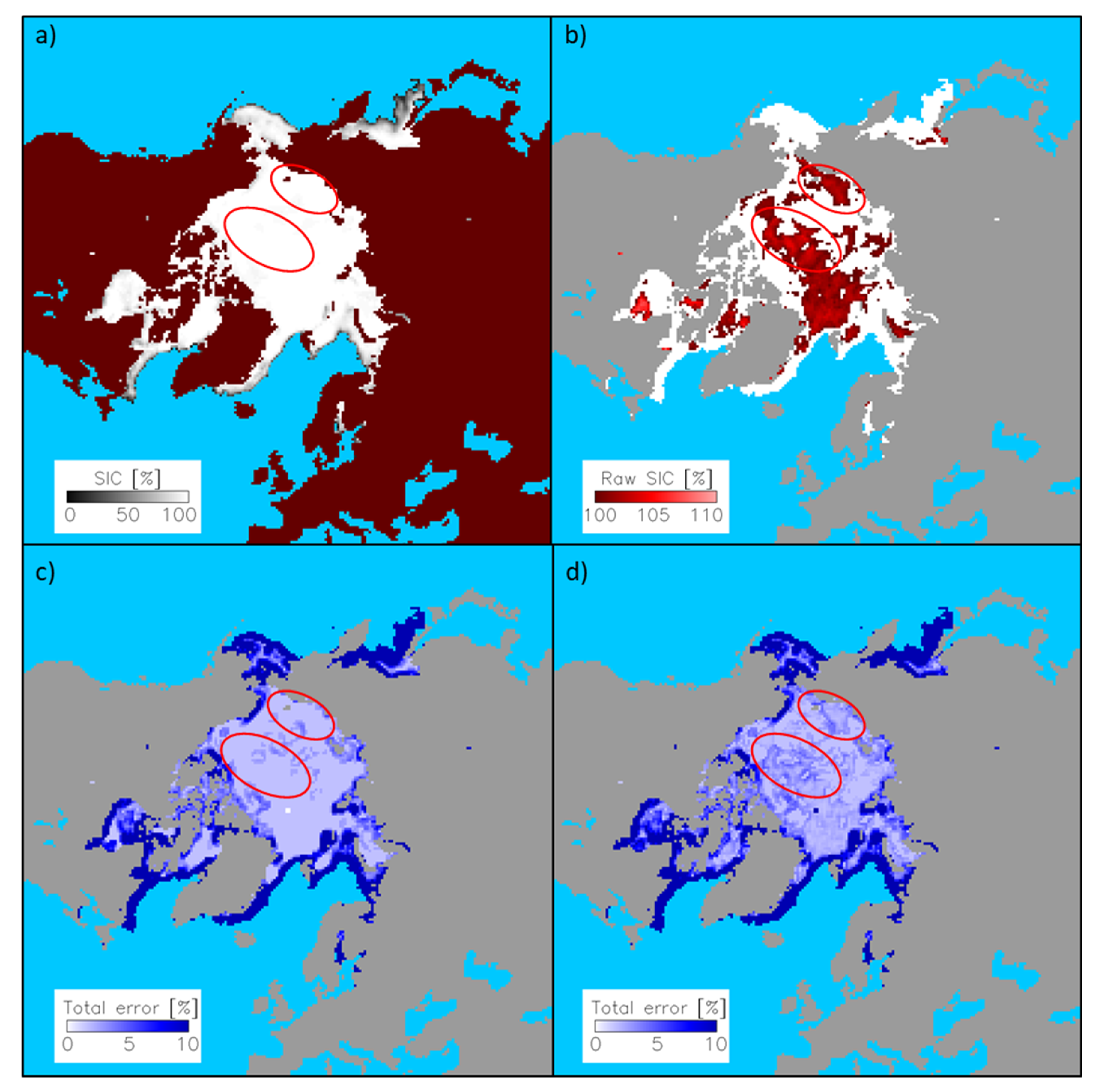
Figure 1. Maps of truncated SIC (a), non-truncated (=Raw) SIC focusing on values >100% (b), the original total error (c) and the corrected (see text) total error (d) of 3 April 2010, in the Northern Hemisphere. Shown are SICCI-50km data. I optimized the range of total error values shown to better illustrate error variations in high-concentration areas; maximum values actually peak at ~40%. Red ellipses highlight two regions with a pronounced fraction of SIC > 100%, indicating in maps (c,d) how the total error changes in response to the correction carried out.
Remotesensing 13 04421 g001
Figure 2. Maps of truncated SIC (a), non-truncated (=Raw) SIC focusing on values >100% (b), the original total error (c) and the corrected (see text) total error (d) of 9 October 2010, in the Southern Hemisphere. Shown are SICCI-50km data. I optimized the range of total error values shown to better illustrate error variations in high-concentration areas; maximum values actually peak at ~40%. Red ellipses highlight two regions with a pronounced fraction of SIC > 100%, indicating in maps (c,d) how the total error changes in response to the correction carried out.
Remotesensing 13 04421 g002
Figure 3. Sample panels illustrating the methodology for SICCI-50km for 26 January 2010, in the Northern Hemisphere. Top two panels show correlation discs (see text) for sea-ice concentration (SIC) error (a) and total error (b). The disc has a radius of 1000 km, and grid cells shown represent 50 km. Middle two panels show the set of hypothetical exponential functions r h y p o ((see Equation (4)) describing the hypothetical exponential decay of the correlation away from the correlation disc’s center (blue dashed), together with the observed mean correlation r i j (solid black) for the SIC error (c) and the total error (d). Only every fifth hypothetical exponential function is plotted. The r h y p o that fits best to r i j is highlighted red. Bottom two panels show the RMSD computed for every exponential function (Equation (5)). The minimum of this curve points to that value of L (see text), which is taken as correlation length scale of the respective parameter, i.e., SIC error (e) and total error (f).
Remotesensing 13 04421 g003
Figure 4. Sample panels illustrating the methodology for SICCI-50km for 16 August, 2010, in the Southern Hemisphere. Top two panels show correlation discs (see text) for sea-ice concentration (SIC) error (a) and total error (b). The disc has a radius of 1000 km, and grid cells shown represent 50 km. Middle two panels show the set of hypothetical exponential functions r h y p o ((see Equation (4)) describing the hypothetical exponential decay of the correlation away from the correlation disc’s center (blue dashed), together with the observed mean correlation r i j (solid black) for the SIC error (c) and the total error (d). Only every fifth hypothetical exponential function is plotted. The r h y p o that fits best to r i j is highlighted red. Bottom two panels show the RMSD computed for every exponential function (Equation (5)). The minimum of this curve points to that value of L (see text), which is taken as correlation length scale of the respective parameter, i.e., SIC error (e) and total error (f).
Remotesensing 13 04421 g004
Figure 5. Illustration of the coverage with correlation discs and the associated RMSD profile derived for the set of exponential functions (see Figure 3) for the SIC error derived from SICCI-50km for the year 2010 for a sample region north of the Canadian Arctic Archipelago in the Northern Hemisphere. Panels are shown every 40 days. Only the map of 7 July is missing because of too few SIC values > 90%.
Remotesensing 13 04421 g005
Figure 6. Maps of the SIC error correlation length scale L in kilometers of SICCI-50km, SICCI-25km and OSI-450 (left three columns) and the total error correlation length scale of OSI-450 (rightmost column) in the Northern Hemisphere for the same dates as used in Figure 5, except August and September.
Remotesensing 13 04421 g006
Figure 7. As Figure 6, but showing the correlation length scale in the Southern Ocean. Here, maps in months December, January and March are missing, while those falling into Austral winter (July, August, September) are all shown. Differences in the spatial extent of valid values, e.g., on 2010-09-25, are caused by the methodological requirements such as the need for a SIC larger than 90%.
Remotesensing 13 04421 g007
Figure 8. Correlation discs obtained for the SICCI-50km SIC error for 26 January of years 2005 through 2010 in the area north of the Bering Strait shown in Figure 3a.
Remotesensing 13 04421 g008
Figure 9. Correlation discs obtained for the SICCI-50km total error for 26 January of years 2005 through 2010 in the area north of the Bering Strait shown in Figure 3b. Note that the correlation in the center of the disc equals 1 and is not shown.
Remotesensing 13 04421 g009
Figure 10. Time series of the average correlation length scale (left column) and RMSD (right column) for a 7 × 7 grid cells area at 50 km (350 km × 350 km) and a 13 × 13 grid cells area at 25 km (325 km × 325 km) north of Wrangell Island for OSI-450 (a,b), SICCI-25km (c,d) and SICCI-50km (e,f). Each panel shows time series for the SIC error correlation length scale and the total error correlation length scale. Zero values denote data gaps due to either missing data files (two days between day of the year 30 and 40 in panels (cf) or due to SIC values dropping below 90% (between day of the year 170 and 275).
Remotesensing 13 04421 g010
Figure 11. Time series of the average SIC error correlation length scale (a) and average total error correlation length scale (b) for the same area north of Wrangell Island used in Figure 10 for SICCI-50km for years 2003 to 2010. The time series of each year is shown at a different gray tone with the most recent year (2010) shown in light gray. Zero values denote data gaps due to either missing data files (two days between day of the year 30 and 40 in 2010) or due to SIC values dropping below 90% (during summer).
Remotesensing 13 04421 g011
Table 1. Overview of the investigated sea-ice concentration products.
ProductInput Data
and Frequencies
Grid Resolution
and Type
Footprint Sizes (for SSMIS and AMSR-E Channels Only)Reference
OSI-450SMMR, SSM/I, SSMIS
19.35 and 37.0 GHz
25 km × 25 km EASE2.070 km × 45 km (19 GHz) and
38 km × 30 km (37 GHz)
[9,13]
SICCI-25kmAMSR-E, AMSR2
18.7 and 36.5 GHz
25 km × 25 km EASE2.027 km × 16 km (18.7 GHz) and
14 km × 9 km (36.5 GHz)
[9]
SICCI-50kmAMSR-E, AMSR2
6.9 and 36.5 GHz
50 km × 50 km EASE2.075 km × 43 km (6.9 GHz and
14 km × 9 km (36.5 GHz)
[9]
Column “Product” holds to the identifier I, used henceforth to refer to the data product, and which algorithm it uses. Column “Input Data and Frequencies” refers to the input satellite data for each product, which comes at grid resolution and type, as listed in the 3rd column. I provide the respective footprint sizes at the used frequencies to illustrate the different native spatial resolutions in the 4th column, followed by the respective references.
Publisher’s Note: MDPI stays neutral with regard to jurisdictional claims in published maps and institutional affiliations.