Melt Pond Retrieval Based on the LinearPolar Algorithm Using Landsat Data

Abstract

The formation and distribution of melt ponds have an important influence on the Arctic climate. Therefore, it is necessary to obtain more accurate information on melt ponds on Arctic sea ice by remote sensing. The present large-scale melt pond products, especially the melt pond fraction (MPF), still require verification, and using very high resolution optical satellite remote sensing data is a good way to verify the large-scale retrieval of MPF products. Unlike most MPF algorithms using very high resolution data, the LinearPolar algorithm using Sentinel-2 data considers the albedo of melt ponds unfixed. In this paper, by selecting the best band combination, we applied this algorithm to Landsat 8 (L8) data. Moreover, Sentinel-2 data, as well as support vector machine (SVM) and iterative self-organizing data analysis technique (ISODATA) algorithms, are used as the comparison and verification data. The results show that the recognition accuracy of the LinearPolar algorithm for melt ponds is higher than that of previous algorithms. The overall accuracy and kappa coefficient results achieved by using the LinearPolar algorithm with L8 and Sentinel-2A (S2), the SVM algorithm, and the ISODATA algorithm are 95.38% and 0.88, 94.73% and 0.86, and 92.40%and 0.80, respectively, which are much higher than those of principal component analysis (PCA) and Markus algorithms. The mean MPF (10.0%) obtained from 80 cases from L8 data based on the LinearPolar algorithm is much closer to Sentinel-2 (10.9%) than the Markus (5.0%) and PCA algorithms (4.2%), with a mean MPF difference of only 0.9%, and the correlation coefficients of the two MPFs are as high as 0.95. The overall relative error of the LinearPolar algorithm is 53.5% and 46.4% lower than that of the Markus and PCA algorithms, respectively, and the root mean square error (RMSE) is 30.9% and 27.4% lower than that of the Markus and PCA algorithms, respectively. In the cases without obvious melt ponds, the relative error is reduced more than that of those with obvious melt ponds because the LinearPolar algorithm can identify 100% of dark melt ponds and relatively small melt ponds, and the latter contributes more to the reduction in the relative error of MPF retrieval. With a wider range and longer time series, the MPF from Landsat data are more efficient than those from Sentinel-2 for verifying large-scale MPF products or obtaining long-term monitoring of a fixed area.

1. Introduction

Melt ponds are some of the most common phenomena on the surface of Arctic sea ice in warm seasons and generally form in late May and refreeze during late August and early September [1]. The distribution and variability of melt ponds have an important influence on the Arctic climate through sea ice albedo feedback [2]. In recent years, it has been shown that the melt pond fraction (MPF) of the Arctic in spring can effectively predict the September minimum sea ice extent [3,4,5], which leads to enhancements in the seasonal forecasting ability of the summer sea ice extent. Therefore, accurately obtaining the MPF is extremely vital for understanding and predicting Arctic sea ice changes.

Compared with field observations and aerial photography, satellite remote sensing has high spatial resolution and temporal continuity. Optical satellite remote sensing data are widely used in MPF retrieval because of their strong intuitive and interpretative capability.

At present, there are two MPF products with 25 km resolution covering the entire Arctic, based on medium-resolution data [6,7,8]. The moderate resolution imaging spectroradiometer (MODIS)-derived MPF product spans from 2000 to 2011 [7], and the medium-resolution imaging spectrometer (MERIS)-derived MPF product spans from 2002 to 2011 [8]. Recently, Ding created new MODIS-based MPF data with a longer period of 2000–2019 [9]. These MPF products cover the entire Arctic but generally have a relatively lower resolution of 12.5 km. Higher-resolution optical satellite remote sensing data are needed to validate these MPF retrieval products, and more details of melt ponds, such as pond size, shape, and color, could be acquired.

MPF retrieval algorithms for high-resolution optical remote sensing products are developed based on the spectral characteristics of melt ponds in the visible and near-infrared bands. Markus et al. [10] used Band 1 (B1, 450–515 nm, blue) and the difference between Band 2 (B2, 525–605 nm, green) and Band 3 (B3, 630–690 nm, red) of Landsat 7 (L7) data in their MPF retrieval algorithm. According to the locations of different surface types in the scatterplot, pure ice/snow, pure melt ponds, and pure open water clusters are defined. The MPF was obtained by calculating the relative distance between the melt pond cluster and others. Rosel et al.’s [11] algorithm transforms the scatterplot of B1 and Band 4 (B4, 775–900 nm, NIR) using principal component analysis (PCA) and then, similar to Markus, determines the thresholds of a 0 MPF and a 100% MPF and calculates the MPF of a certain pixel by its distance to the trinary pixel cluster. These two algorithms assume that the albedo of different melt ponds is a fixed value in certain bands. However, this assumption is not consistent with observations that the albedo or reflection of melt ponds changes significantly [12,13,14] and causes the underestimation of the value of retrieved MPF. Given this aspect, Wang et al. [15] proposed the LinearPolar algorithm using B2 (457–522 nm, blue, corresponding to B2 (450–515 nm, blue) of Landsat 8 (L8)) and Band 8 (B8, 784–900 nm, NIR, corresponding to B5 (845–885 nm, NIR) of L8) of Sentinel-2A (S2) data with a resolution of 10 m. In this band combination, the pure ice/snow pixels and the pure melt ponds pixels are approximately distributed along two corresponding straight lines, and the albedo of different melt pond pixels is not fixed. In the work of Wang et al., by considering the coordinates of B2 and B2–B8, the intersection of the lines is taken as the pole. The baseline is the axis of melt ponds with 100% MPF, and the other line is the axis of ice/snow with 0 MPF. The (polar) angle between the lines is the MPF. Then, the axis of ice/snow (0 MPF, located at the bottom of the pure ice/snow pixels) and the axis of melt ponds (100% MPF, located at the top of the pure melt pond pixels) parallel to the horizontal axis can be obtained by polar coordinate transformation. This means that although the albedo of melt pond pixels is not fixed, its θ (the angular coordinate of pixels after polar coordinate transformation, that is, the included angle between pixels and 100% melt pond axis in polar coordinate) is the same, which is the difference between the LinearPolar algorithm and the previous algorithms. The MPF can be calculated by the distance between the two axes. This algorithm takes into account the change in melt pond albedo of different colors, which improves the accuracy of the MPF of dark-blue melt ponds.

Since Landsat data have been used for many MPF validations with a low resolution previously with different algorithms, it is necessary to apply the LinearPolar algorithm to Landsat data. Since 2003, a hardware component failure left spaces of missing data on either side of L7′s images, which seriously affects the use of L7. Therefore, we chose L8 (the latest Landsat satellite) data to implement the algorithm. Even if the temporal resolution of L8 (16 days) is less than that of S2 (5 days for double satellites, 10 days for a single satellite) and its spatial resolution (30 m) is also lower than that of S2 (10 m), the MPF of some L8 pixels can be up to 100% during the melt season; therefore, the LinearPolar algorithm can be applied to L8 data, and this application could cover a larger area, thereby improving the verification efficiency.

In recent years, the extended melt season has led to more active navigation in the Arctic Passage [16]. The Northwest Passage (NWP) is one of the passages with increased navigability, and it crosses the Canadian Arctic Archipelago (CAA). The northern branch of the NWP is generally covered by multiyear ice (MYI), while the southern channels are generally covered by seasonal sea ice [17]. Since the MPF is related to the summer sea ice melting process [14], the melt pond information of the CAA can enrich our understanding of the regional summer sea ice melting process and provide information for the opening of the NWP. By applying the LinearPolar algorithm to Landsat 8, we explored the algorithm’s feasibility on very high-resolution data. In addition, we obtained the MPF with a more extensive spatial range and high resolution to verify medium- and low-resolution MPF products.

2. Data

We use four L8 scenes and six S2 scenes of the corresponding location. These images were all obtained from the beginning to the end of July, the middle of the melt season, in the west of CAA (Figure 1). Three L8 scenes are located in the northern MYI area, and one L8 scene is located in the southern seasonal sea ice area. The data from this time and location are selected because, on the one hand, it is based on the consideration of the amount of data. On the other hand, there are more dark melt ponds and light melt ponds in this period [14]. Using data in this period can highlight the advantages of the LinearPolar algorithm.

2.1. L8 Data

L8 data are obtained from the United States Geological Survey (USGS) [18]. L8 includes B1–B7 and B9 with a resolution of 30 m and B8 with a resolution of 15 m. The LinearPolar algorithm [15] was applied to L8, B2 (450–515 nm), B3 (525–600 nm), B4 (630–680 nm), and B5 (845–885 nm) in the experiments in this paper. The temporal resolution of L8 is 16 days, and the temporal range is from 2013 to the present.

2.2. Sentinel-2A Data

S2 level 1C (L1C) data (hereafter, S2) are available for download from the European Space Agency (ESA) [19] and were used as the validation data. S2 includes 13 bands covering visible bands, near-infrared bands, and shortwave infrared bands, with resolutions of 10 m (B2, B3, B4, and B8), 20 m (B5, B6, B7, B8a, B11, and B12), and 60 m (B1, B9, and B10). B2 (457–522 nm) and B8 (784–900 nm) are used for the LinearPolar algorithm following Wang et al. [15]. The S2 mission comprises a constellation of two polar-orbiting satellites, and the revisit time is 10 days at the equator with one satellite and 5 days with two satellites. The temporal range is from 2015 to the present.

2.3. Data Process

In this paper, we randomly selected four L8 scenes (black frame in Figure 1) obtained during July over the western CAA under almost clear sky conditions (cloud cover less than 5%). The selected 6 S2 scenes correspond to the same time and location as the L8 scenes (red dashed frame in Figure 1). The seasonal pond evolution is generally divided into four stages. In the third stage, the melt pond develops steadily and is widely distributed. The MPF often reaches the seasonal maximum [14]. Recent studies show that the third stage of pond evolution is generally from the end of June to the beginning of August [9]. Therefore, the images used in this paper are all obtained from the beginning to the end of July. S2 and L8 data have coincided since June 2015. The temporal resolutions of L8 and S2 are 16 days and 5 days, respectively. Taking a small area near the western CAA in July 2019 as an example, there are 6 L8 scenes and 23 corresponding S2 scenes with cloud cover less than 5%. There is an large number of data of the whole CAA region from May to September during 2015–2021. In this paper we only select several representative scenes for research.

We used almost all the overlapping areas of four L8 and six S2 samples (hereafter, six overlapping samples) to select the best band combination. At the same time, considering that the number of pixels of ice and snow greatly exceed those of melt ponds, we randomly selected 80 pairs of samples with the same location and area size from the S2 and L8 data for the application of the LinearPolar algorithm. Each L8 sample had a size of 30 × 20 pixels and a resolution of 30 m, and each S2 sample had a size of 90 × 60 pixels and a resolution of 10 m. In the 80 randomly selected cases, the distribution of surface types is random, which is suitable to draw a generalizable conclusion.

3. Methods

3.1. Band Combination Experiments

Following Wang et al.’s [15] work, we first chose a training area to discriminate typical pixels of different surface types. The same training areas were selected for the S2 data and L8 data, and the training samples were selected at the corresponding locations by visual inspection based on the true color images, as shown in Figure 2. There are 7 categories on the sea ice surface: bare ice, snow-covered ice, open water, melt pond 1 (light-blue pond), melt pond 2 (dark-blue pond), mixed pixel 1 (snow-covered ice and melt pond 1), and mixed pixel 2 (snow-covered ice and melt pond 2) (Figure 2). The two kinds of mixed pixels are located at the edge of the two kinds of melt ponds.

For the S2 data of Figure 2a, B2 (457–522 nm) and B8 (784–900 nm) are used in the LinearPolar algorithm [15] to obtain a scatterplot of B2 and the difference between B2 and B8 (B28), in which the ice/snow pixels and melt pond pixels are distributed along two lines, and two types of mixed pixels are located between these two lines (Figure 3a). The intersection of these two lines is taken as the origin of polar coordinates, and the values of B28 and B2 are transformed to polar coordinate values (Figure 3b). The bare ice and snow are located on one line (sea ice axis), which was set to 0 MPF (the threshold of the sea ice axis is denoted by ${\theta }_t$), and two types of melt ponds are located on another line (melt pond axis), which was set to 100% MPF (the threshold of the melt pond axis is denoted by ${\theta }_{t0}$). Both lines are parallel to the horizontal axis; therefore, the thresholds of the sea ice axis and melt pond axis can be determined.

In Figure 3, we use the DN values to obtain the scatterplots. The conversion process from DN value to reflectance is as follows:

$$L_{\lambda }=Grescale\times QCAL+Brescale, {\rho }_p=\frac{\pi \times L_{\lambda }\times d^2}{ESU{N}_{\lambda }\times \cos {\theta }_s}$$

(1)

where $L_{\lambda }$ is the TOA radiance; $Grescale$ is the reflectance multiplicative scaling factor for the band; $Brescale$ is the reflectance additive scaling factor for the band; $QCAL$ is the level 1 pixel value in DN; ${\rho }_p$ is the surface reflectance (albedo); $d$ is the Earth–Sun distance; $ESU{N}_{\lambda }$ is the mean solar exoatmospheric irradiances; and ${\theta }_s$ is the solar zenith angle.

For the application of the LinearPolar algorithm [15] on L8, a series of experiments are conducted to determine the most suitable band combination. The selection of the best band combination of the LinearPolar algorithm on L8 mainly refers to four aspects: the albedo difference of melt ponds and other surface types in the visible to the near-infrared band, the band combination used in the previous algorithms, the errors (the MPF errors, the confusion matrix accuracy, and the standard deviation caused by the threshold change) of the retrieval results of the LinearPolar algorithm with different band combinations, and the dispersion of pixels near the melt pond axis and sea ice axis after the polar coordinate change. According to the characteristics of the LinearPolar algorithm, the smaller the pixel dispersion, the more accurate the determination of the threshold and the higher the retrieval accuracy.

According to the spectral albedos for different surface types on Arctic sea ice (Figure 4), the albedos of bare ice and snow are much greater than those of melt ponds. From the visible light band (B2, B3, and B4) to the near-infrared band (B5), the albedos of these types show a downward trend, and the albedos of melt ponds decrease more sharply than those of bare ice and snow. Thus, the melt ponds can be distinguished from bare ice and snow by the difference in albedos between the visible light band and near-infrared band. Figure 4 shows that a relatively obvious difference exists between B2 and B5 for L8. At the same time, considering the B2–B34 (the difference between B3 and B4, approximately 0.5–1.7 less than B25) combination in the Markus algorithm and B2–B5 combination in the PCA algorithm, 4 alternative band combinations of B2–B34, B2–B5, B2–B25 (the difference between B2 and B5), and B5–B25 are used in the experiments.

Subsequently, the scatterplots of these four combinations were obtained and then transformed into polar coordinates (Figure 5). To be consistent with Figure 3, the DN value is still used to obtain the scatterplots in Figure 5. For B2–B34, the melt pond clusters cannot be regarded as a line, and the lead cluster span is too large to remove. The point distributions of the other three combinations except B2–B34 are all reasonable: sea ice/snow points and all melt pond points are consistent in a straight line, and only the distance between the two axes varies.

To select the best band combination, we made the following statistics: First, we calculated the error of the MPF retrieval results between L8 and S2 of four combinations for 6 overlapping samples. The error analysis (

Table 1. The errors for the MPF retrieval results of the four band combinations between L8 and S2.

Band Combination	MPF (%)	ME (%)	MAE (%)	RMSE (%)	STD (%)
B2–B5	11.22	−2.32	10.38	16.39	16.02
B2–B25	12.75	−0.71	10.35	16.22	16.05
B2–B34	9.95	−3.51	10.63	16.88	16.22
B5–B25	12.59	−0.87	10.63	16.61	16.13

ME: mean error; MAE: mean absolute error; RMSE: root mean square error; and STD: standard deviation.

) shows that all the errors (mean error (ME), mean absolute error (MAE), root mean square error (RMSE), and standard deviation (STD)) of the retrieval results of the four combinations and S2 are within the acceptable range. The differences in errors for all 4 combinations are minimal, but it is obvious that the band combination of B2–B25 is relatively better than that of other combinations.

Second, to quantitatively evaluate the performance of different band combinations when the LinearPolar algorithm is applied to L8, we randomly selected 1500 pixels in areas with melt ponds of each overlapping image, with a total of 9000 verification points. Taking the retrieval results of S2 using the LinearPolar algorithm as the true categories, the results of different L8 band combinations are evaluated by a confusion matrix.

Table 2. Quantitative comparison of the results of different band combinations.

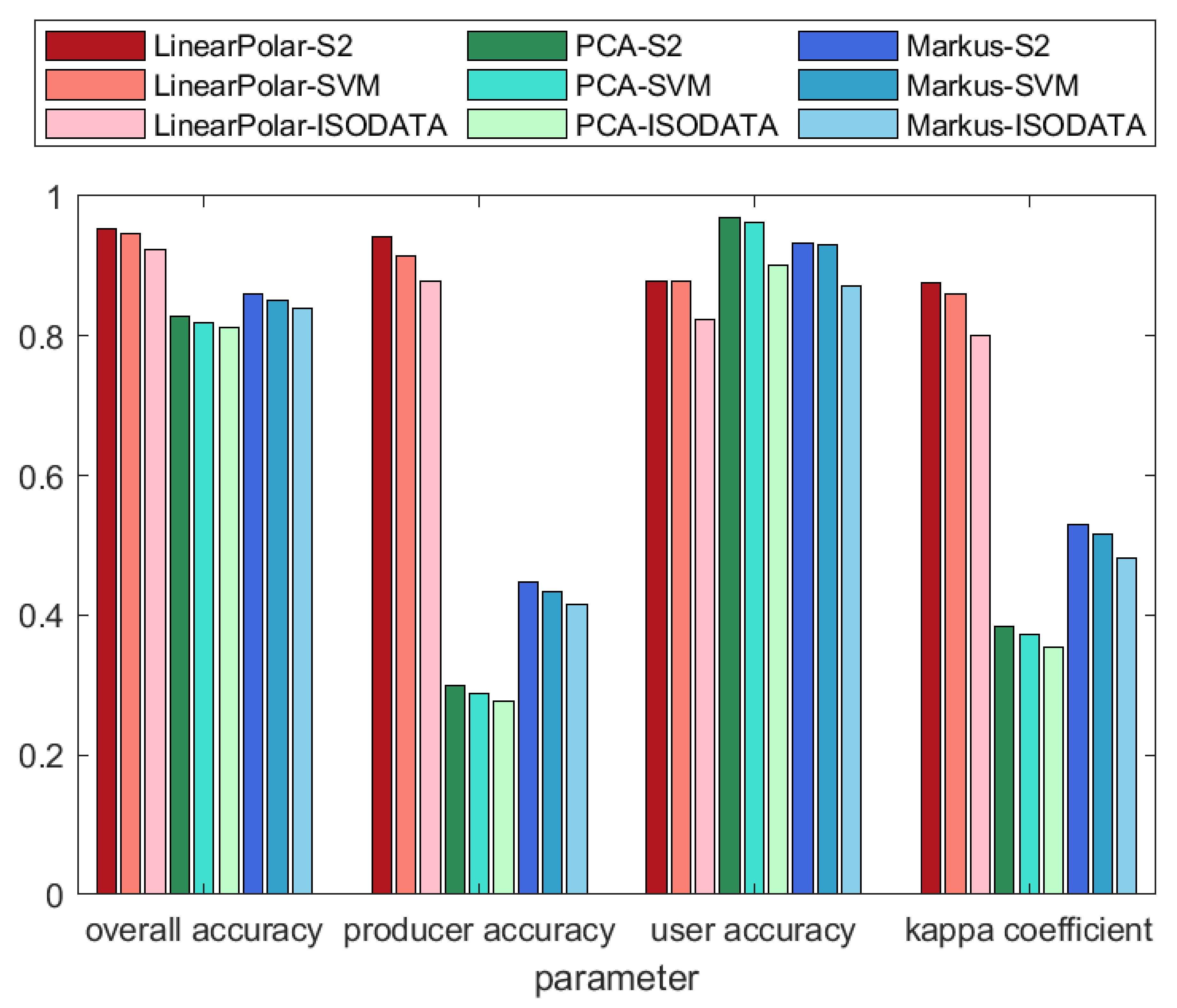
Band Combination	Producer’s Accuracy (%)	User’s Accuracy (%)	Overall Accuracy (%)	Kappa Coefficient
B2–B5	80.93	94.58	94.20	0.8384
B2–B25	90.77	91.92	95.79	0.8842
B2–B34	81.76	92.20	93.91	0.8265
B5–B25	91.88	90.21	95.58	0.8797

shows the results for the producer’s accuracy, the user’s accuracy, the overall accuracy, and the kappa coefficient for different band combinations.

The overall accuracy of the four band combinations is more than 90%, and the kappa coefficient is also greater than 0.8, indicating that the classification results are highly consistent. B2−B25 and B5−B25 have similar overall accuracies and kappa coefficients and perform better than those of the other combinations.

When applying the LinearPolar algorithm in batch processing, the Hough transform is used to automatically determine the threshold. In this paper, since only several scenes are used rather than the entirety of scenes, it is more accurate to determine the threshold manually. Third, to select the best combination, we also conducted threshold sensitivity experiments on these 4 combinations. The sea ice axis threshold ${\theta }_t$ is transformed by $\pm 3\%$ for each combination, and then, we calculated the standard deviation of the retrieval results of the 4 band combinations after the threshold change (

Table 3. Comparison of the MPF variations for the 4 band combinations with threshold variations of ±3% and ±5% for 6 overlapping areas.

Band Combination	B2–B5		B2–B25		B2–B34		B5–B25
Threshold	−3%	+3%	−3%	+3%	−3%	+3%	−3%	+3%
STD (%)	1.23	1.17	1.20	1.14	1.22	1.19	1.22	1.18
Threshold	−5%	+5%	−5%	+5%	−5%	+5%	−5%	+5%
STD (%)	2.01	1.58	1.97	1.80	1.99	1.88	2.01	1.87

STD: standard deviation.

). It can be seen that the error difference caused by the threshold transformation of the four band combinations is also small, but relative to other combinations, the B2–B25 combination is the best.

Last, standard deviation was used to describe the pixel dispersion of the melt pond axis and sea ice axis (

Table 4. Standard deviation of the melt pond axis and ice/snow axis for the 4 band combinations.

Band Combination	B2–B5		B2–B25		B2–B34		B5–B25
Axis	Ice/ snow	Melt pond	Ice/ snow	Melt pond	Ice/ snow	Melt pond	Ice/ snow	Melt pond
STD (%)	0.65	0.79	0.55	0.42	0.67	1.24	1.44	0.87

STD: standard deviation.

). The results show that the pixel distribution of the B2–B25 band combination is the most compact, which indicates a minimum error is achieved in the threshold determination. Overall, the band combination of B2–B25 is better than those of other combinations. This also suggests that the band combination selected in Wang et al. (2020) is the best.

3.2. Retrieval Algorithm

The MPF of L8 for each pixel can be calculated by the following equation, which was modified from Wang et al. (2020):

$$\left\{\begin{array}{c}0,\theta >{\theta }_t\\ \frac{{\theta }_t-\theta }{{\theta }_t-{\theta }_{t0}},0<\theta <{\theta }_t\\ 1,\theta <{\theta }_{t0}\end{array}\right., \left\{\begin{array}{c}\theta =\arctan \left[\frac{b_2-y_0}{b_{25}-x_0}\right]-\arctan \left[\frac{b_{2-\mathrm{mp}1}-y_0}{b_{25-\mathrm{mp}1}-x_0}\right]\\ r=\sqrt{{\left(b_{25}-x_0\right)}^2+{\left(b_2-y_0\right)}^2}\end{array}\right.$$

(2)

where θ is the angular coordinate; ${\theta }_t$ and ${\theta }_{t0}$ are the thresholds of the sea ice axis and melt pond axis, respectively; r is the radial coordinate; $\left(x_0,y_0\right)$ is the Cartesian coordinates of the polar origin; $b_2$ and $b_{25}$ are the reflectance of B2 and the difference between B2 and B5 (B2–B5), respectively; $b_{2-\mathrm{mp}1}$ and $b_{25-\mathrm{mp}1}$ are the mean values of the melt pond 1 reflectance of $b_2$ and $b_{25}$ in a training area (the corresponding values of melt pond 2 are same as those of melt pond 1).

The thresholds are determined by the Hough transform [21] from Wang et al.’s [15] work. However, the Hough transform requires enough sample data. There are fewer pixels in the same region of L8 than S2; therefore, the thresholds of L8 are determined manually here. Of course, the training region can also be expanded, and then the Hough transform can be used.

3.3. Verification and Comparison Methods

The resolution of S2 is higher than that of L8; therefore, the S2 data are used as the verification data. In this paper, we use the LinearPolar algorithm (on the S2 data), support vector machine (SVM) algorithm and iterative self-organizing data analysis technique (ISODATA) algorithm to verify and compare the results.

The MPF obtained from S2 using the LinearPolar algorithm is taken as one of the standards to verify the MPF obtained from L8, and the retrieval process follows Wang’s [15] work. For the convenience of comparison, the MPF results of S2 were interpolated into the 30 m resolution grid of L8.

As a supervised classification algorithm, the SVM classification result is determined only by the appropriate category samples selected manually, which is helpful for identifying the key features of categories [22]. The SVM algorithm is simple and robust; however, it is difficult to implement on large-scale classification samples, and manual selection is too subjective. Since SVM classification cannot identify pixel values but can only roughly classify categories with a range of values, all the pixels were divided into melt ponds (main components), open water (main components), and ice/snow (main components). Then, the SVM classification results of S2 were interpolated into the L8 grid.

ISODATA [23], a mature unsupervised classification algorithm, does not need manual initial input but needs to manually adjust the merged categories after the classification; this algorithm is more automatic than SVM. For ISODATA, we set the number of classes to 15, the maximum number of iterations to 10, the change threshold to 1, the minimum class distance to 1, and the maximum merge pairs to 1 and then manually merged the 15 categories into 3 categories: melt ponds, ice/snow, and open water. The ISODATA classification results of S2 were interpolated into the grid of L8.

4. Results

Figure 6 shows the retrieval results of five cases, which have obvious melt ponds, randomly selected from the coincidence part of scene D (L8) and scene f (S2) in Figure 1. For the retrieval results of L8 using the LinearPolar algorithm, these three MPFs of S2, SVM, and ISODATA are used to verify and compare.

The classification data of the SVM and ISODATA algorithms are shown in Figure 6(c1–c5) (the interpolation of the S2 classification data by the SVM algorithm) and Figure 6(e1–e5) (the interpolation of the S2 classification data by the ISODATA algorithm, Figure 6d1–d5). The MPF retrieval data of S2 using the LinearPolar algorithm are shown in Figure 6(f1–f5), and Figure 6(g1–g5) shows the interpolation of Figure 6(f1–f5) onto the L8 grid. The distribution of the three algorithms (the SVM algorithm, the ISODATA algorithm, and the LinearPolar algorithm) data are approximate. They can identify the 100% dark-blue melt ponds (cases 2, 3, and 4) and light-blue melt ponds (cases 1 and 5).

The three MPF data of S2 are compared with the true-color images of each case. In cases 1–3 and case 5, which have lead, all three algorithms incorrectly classify the submerged ice beside the lead as a melt pond, which leads to a high MPF. For cases 2, 4, and 5, which have many relatively small melt ponds, the SVM and ISODATA algorithms are almost unable to identify these melt pond points. The reason is when the melt pond points are selected manually, only the pixels with the melt pond accounting for the main part are selected, while the S2 data using the LinearPolar algorithm can calculate the MPF of this part.

The previous algorithms, the Markus algorithm (Markus et al., 2003), the PCA algorithm (Rosel et al., 2011), and the LinearPolar algorithm were all applied to the L8 data to obtain the retrieved MPF (Figure 6(h1–h5, i1–i5, and j1–j5), respectively).

As shown in Figure 6, case 1 and case 5 are similar, with obvious light-blue melt ponds. Compared with Figure 6(g1,g5), 100% of the melt ponds in the two cases can be identified by all three algorithms. However, for cases 2–4 with dark-blue melt ponds, compared with the true-color images, only the LinearPolar algorithm can identify the dark melt ponds with a 100% MPF as 100% MPF. The relatively small melt ponds in the five cases can be identified only by the LinearPolar algorithm.

Table 5. The average MPF of the 5 cases using the three algorithms on L8 and one algorithm and two classification algorithms on S2.

Case	MPF (%)
	L8_Markus	L8_PCA	L8_LinearPolar	S2_LinearPolar	SVM	ISODATA
1	2.8	3.0	5.9	6.6	7.4	7.5
2	4.1	4.6	10.7	12.1	13.6	11.1
3	3.5	3.8	10.7	10.7	8.8	8.9
4	7.0	7.1	13.8	14.3	12.4	11.6
5	2.5	2.8	5.5	5.9	5.6	5.0
mean	3.98	4.26	9.32	9.92	9.56	8.82

shows the average MPF results of the five cases from three retrieval algorithms using L8 data and the average MPF data of the five cases from the interpolation of a retrieval algorithm and two classification algorithms using S2 data (See Appendix B for specific average error of 80 cases). Consistent with the conclusion drawn in Figure 6, the average MPFs of the three validation data are relatively similar for each case. The correlation coefficient between the two classification data is 0.96, and the mean bias is 0.7%. The correlation coefficients between the retrieval data of S2 and the two classification data are as high as 0.90 and 0.95, and the mean biases are 0.4% and 1.1%. From Figure 7 and the comparison of the true-color images, we found that the S2 data using the LinearPolar algorithm have a stronger ability to capture relatively small melt ponds, especially small melt ponds surrounded by ice and snow. The statistics show that the classification data are affected for this reason.

Among the three retrieval results of L8 using different algorithms, the results of the LinearPolar algorithm are the closest to those used for verification, and the mean error with S2 using the LinearPolar algorithm, SVM algorithm, and ISODATA algorithm are −0.6%, −0.24%, and 0.5%, respectively. The other two algorithms seriously underestimated the MPF of each case, and the mean errors were −5.9%, −5.6%, and −4.8%, respectively, for the Markus algorithm and −5.7%, −5.3%, and −4.6%, respectively, for PCA. Therefore, the MPF is underestimated by these two algorithms. Overall, the MPF obtained from the LinearPolar algorithm, which is most similar to the Sentinel-2A result, SVM result, and ISODATA result, is more accurate than previous algorithms.

The above analysis shows that the three S2 data (the LinearPolar algorithm data, the SVM algorithm data, and the ISODATA algorithm data) are relatively similar. We further use the confusion matrix (

Table 6. Quantitative comparison of the results of different algorithms with 3 validation data.

Data	True Class (S2)	Algorithm (L8)	Producer’s Accuracy (%)	User’s Accuracy (%)	Overall Accuracy (%)	Kappa Coefficient
1	LinearPolar	LinearPolar	97.55	84.60	93.40	0.86
		PCA	54.49	99.63	85.07	0.62
		Markus	65.10	96.08	87.73	0.70
	SVM	LinearPolar	97.63	80.35	91.87	0.82
		PCA	56.99	98.88	86.47	0.64
		Markus	68.17	95.48	89.13	0.72
	ISODATA	LinearPolar	98.97	67.79	87.60	0.72
		PCA	66.41	95.90	90.60	0.73
		Markus	75.71	88.25	91.13	0.76
2	LinearPolar	LinearPolar	98.54	90.92	91.80	0.80
		PCA	13.55	100.00	40.53	0.09
		Markus	35.09	96.00	54.13	0.23
	SVM	LinearPolar	96.97	92.00	91.80	0.80
		PCA	13.18	100.00	38.67	0.09
		Markus	34.22	96.27	52.67	0.22
	ISODATA	LinearPolar	94.11	93.44	90.73	0.76
		PCA	12.59	100.00	35.53	0.08
		Markus	32.79	96.53	49.60	0.19
3	LinearPolar	LinearPolar	88.10	81.42	91.93	0.79
		PCA	25.27	88.46	94.80	0.36
		Markus	36.26	76.74	95.47	0.48
	SVM	LinearPolar	85.17	81.42	91.07	0.77
		PCA	17.42	88.46	92.27	0.28
		Markus	25.76	79.07	92.87	0.36
	ISODATA	LinearPolar	85.20	74.57	89.53	0.73
		PCA	15.17	84.62	91.33	0.25
		Markus	22.76	76.74	91.87	0.32
4	LinearPolar	LinearPolar	93.69	95.08	91.87	0.80
		PCA	10.79	100.00	85.20	0.17
		Markus	18.26	91.67	86.60	0.27
	SVM	LinearPolar	93.59	94.81	91.60	0.79
		PCA	10.16	96.15	84.87	0.16
		Markus	17.48	89.58	86.13	0.25
	ISODATA	LinearPolar	92.84	93.88	90.40	0.76
		PCA	9.23	92.31	84.07	0.16
		Markus	16.15	87.50	85.07	0.23
5	LinearPolar	LinearPolar	86.30	84.56	97.13	0.84
		PCA	43.84	100.00	93.93	0.56
		Markus	50.68	93.67	94.87	0.63
	SVM	LinearPolar	81.70	83.89	96.53	0.81
		PCA	41.83	100.00	93.47	0.54
		Markus	48.37	93.67	94.40	0.61
	ISODATA	LinearPolar	86.30	84.56	97.13	0.84
		PCA	41.30	59.38	91.73	0.43
		Markus	45.65	53.16	91.93	0.45
6	LinearPolar	LinearPolar	89.44	86.75	97.33	0.86
		PCA	79.50	88.89	96.60	0.82
		Markus	82.61	85.26	96.53	0.82
	SVM	LinearPolar	84.62	86.14	96.67	0.83
		PCA	74.56	87.50	95.80	0.78
		Markus	78.11	84.62	95.87	0.79
	ISODATA	LinearPolar	77.09	83.13	95.33	0.78
		PCA	67.60	84.03	94.47	0.72
		Markus	70.95	81.41	94.53	0.73

) to prove that all three data can be used as verification data.

We randomly selected 1500 pixels of each image in areas with melt ponds, with a total of 9000 verification points. Taking the retrieval data of S2 using the LinearPolar algorithm, SVM classification data, and ISODATA classification data as the true categories, the results of L8 using three different retrieval algorithms are evaluated by confusion matrices. The overall accuracy and kappa coefficient of each image were calculated, as shown in Table 6. Figure 7 shows the overall accuracy and kappa coefficient of 9000 points.

Figure 7 shows that regardless of any type of validation data, the overall accuracy and kappa coefficient of L8 retrieval results using the LinearPolar algorithm are much higher than those of PCA and Markus algorithms. Since both L8 and S2 use the LinearPolar algorithm, the highest accuracy (95.38% and 0.88) is reasonable. The SVM classification data are obtained according to the manually selected typical pixel classification, and the classification data are relatively accurate. Therefore, the accuracy (94.73% and 0.86) of the comparison between the results of L8 using the LinearPolar algorithm and SVM classification data is also relatively high.

The overall accuracy represents the probability of the correct classification of all pixels. The overall accuracy difference of the three algorithms is not too large, and the LinearPolar algorithm performs the best, which means that its calculation results are more accurate. The producer’s accuracy of melt ponds represents the probability of the real melt pond category being identified by the algorithm. The producer’s accuracies of L8 using the LinearPolar algorithm between S2 using the LinearPolar algorithm, the SVM classification algorithm, and the ISODATA classification algorithm are 94.20%, 91.49%, and 87.82%, respectively, which are much higher than the other two algorithms. This shows that the LinearPolar algorithm can identify more melt ponds than PCA and Markus algorithms. The user’s accuracy of melt ponds represents the probability that the melt pond category identified by the algorithm is a real pond category. The result of L8 using the LinearPolar algorithm is slightly lower than that of the other two algorithms. However, this does not contradict our previous results, although the user’s accuracies of the other two algorithms are slightly higher than that of the LinearPolar algorithm, this is because they can only identify a small number of the melt pond pixels. The kappa coefficient is used to evaluate the accuracy of classification. The more consistent the classification results are with the verification data, the higher the kappa coefficient is. The kappa coefficient of L8 using the LinearPolar algorithm is approximately 0.8–0.9, which means the L8 results using the LinearPolar algorithm and the verification data are almost in perfect agreement. The results of the other two algorithms are only in moderate agreement. Therefore, the results of the LinearPolar algorithm are more accurate than those of previous algorithms.

Overall, the results of Table 5 and Table 6 and Figure 7 show that the three S2 data (the LinearPolar algorithm data, the SVM data, and the ISODATA data) are relatively similar; therefore, any of the three MPF data can be used for validation.

Among them, the data of the LinearPolar algorithm indicate that it can identify small-scale melt ponds and requires the least manual intervention. Compared with the other two data (the SVM data and the ISODATA data), the retrieval of the LinearPolar algorithm requires less time and has higher verification efficiency. Moreover, the SVM and the ISODATA algorithms can only determine the category of pixels, while the LinearPolar algorithm can obtain an accurate MPF value of each pixel. Therefore, to further quantify the accuracy of the algorithm, we choose the data of the LinearPolar algorithm to verify the retrieval result of L8.

Figure 8 shows the average MPF of 80 cases using different algorithms (See Appendix A for specific MPF values and RMSE of 80 cases). The errors of the average MPF for the 80 randomly selected cases are shown in

Table 7. The errors of the average MPF for 80 cases between the 3 algorithms for the L8 data and LinearPolar for the S2 data.

(%)	L8_LinearPolar			L8_PCA			L8_Markus
	All	With OMPs	Without OMPs	All	With OMPs	Without OMPs	All	With OMPs	Without OMPs
RMSE	8.5	9.1	7.9	11.7	12.6	10.7	12.3	13.2	11.2
ME	−0.9	−1.4	−0.3	−6.7	−6.9	−6.5	−5.9	−5.6	−6.3
MAE	5.4	5.6	5.2	7.4	7.8	6.9	7.6	8.0	7.1
RE	8.1	10.8	3.2	61.5	52.5	77.9	54.6	42.8	76.3

RMSE: root mean square error; MAE: mean absolute error; ME: mean error; RE: relative error; all: all 80 cases; with OMPs: 43 cases with OMPs; and without OMPs: 37 cases without OMPs.

. The average MPF for the S2 data is 10.9%, and the average MPFs for the L8 data are 10.0%, 5.0%, and 4.2% for the LinearPolar, Markus, and PCA algorithms, respectively. The correlation coefficients of the LinearPolar, PCA, and Markus algorithm results with the S2 data are 0.95, 0.88, and 0.91, respectively. It is obvious that all the errors (RMSE, ME, MAE, and relative error (RE)) of the LinearPolar algorithm are the lowest. The RMSE of the LinearPolar algorithm is 30.9% and 27.4% lower than that of the Markus algorithm and PCA algorithm, respectively. The MAEs of the LinearPolar algorithm are 2.0% lower than those of the Markus algorithm and 2.2% lower than those of the PCA algorithm. The retrieval error of the LinearPolar algorithm is 46.6% lower than that of the Markus algorithm and 53.5% lower than that of the PCA algorithm.

Among the 80 samples selected, 43 samples had obvious (relatively large scale; in this paper, melt ponds with widths greater than 100 m are considered relatively large melt ponds) dark- or light-blue melt ponds, and 37 samples had no obvious (relatively small) melt ponds. Next, we divided all the cases into two categories to calculate the errors (Table 7). Whether there is an obvious melt pond (OMP) or not, the MAE of the LinearPolar algorithm is approximately half of that of the other two algorithms. Regarding the RE, for the samples without OMPs, the LinearPolar algorithm has a mean MPF of 8.1, which is approximately 4 times that of the other algorithms. This finding indicates that the LinearPolar algorithm can identify relatively small melt ponds, which is not possible by the other two algorithms. For the region with OMPs, the RE of the LinearPolar algorithm is approximately 4 or 5 times smaller than that of the other two algorithms but is not reduced by as much as that of the region without OMPs. The reason is the other two algorithms can identify 100% of the light-blue melt ponds but cannot identify 100% of the dark-blue melt ponds, and the retrieval results would be seriously underestimated. In general, the LinearPolar algorithm greatly reduces the retrieval relative error, and the region without OMP performs even better.

5. Discussion

Regardless of the retrieval results of the five cases in Figure 5 or the average MPF of the 80 cases in Table 5, the retrieval results of L8 with a resolution of 30 m using the LinearPolar algorithm are smaller than those of S2 with a resolution of 10 m using the same algorithm. For the same area, Buckley [24] found that the MPFs of 100% of S2 images (resolution: 10 m) were in the range of 0–25%, while only 90% of NASA IceBridge Digital Mapping System (DMS) images (resolution: 0.1 m) were between 0–25%, and 10% of the DMS images were in the range of 25–60%. This finding shows that the higher the resolution is, the higher the MPF for the same retrieval algorithm. In this paper, the S2 data have higher resolution; therefore, the MPF retrieved by the LinearPolar algorithm is higher. The reason is that the high-resolution image can capture more sea ice variability on a smaller scale; that is, the relatively small melt ponds that can be observed in S2 (10 m) images cannot be fully captured or even cannot be captured in L8 (30 m) images in this paper.

In the 80 cases, compared with the Markus and PCA algorithms, the RE of the LinearPolar algorithm is greatly reduced. When the 80 cases were divided into two categories according to whether there were OMPs, the RE of the cases without OMPs decreased more than that of the cases with an OMP. That is, the accurate identification of relatively small melt ponds made a greater contribution to the reduction in the RE of the MPF retrieval.

The pixels surrounding the edge of leads are very special; although there may be sea ice at the bottom of this kind of pixel, which leads to the optical characteristics between the melt pond and lead, it cannot be identified as melt ponds because of the connection between the side and the open water. These pixels are divided into melt ponds during retrieval, which might cause the overestimation of the MPF. This error can be corrected by subtracting the corresponding proportion of the MPF after determining the shape and size of the lead. In this paper, we found that the error caused by submerged ice in the 80 cases (submerged ice appears only in cases with a lead) is small, and this overestimation exists in all algorithms in this paper; therefore, it can be ignored.

Because of the longer time series and larger coverage of Landsat than Sentinel, the efficiency of verification of the lower-resolution MPF is increased. It is helpful to understand the long-term variation trend in sea ice in fixed areas. The successful application of the LinearPolar algorithm in the Landsat data implies that this algorithm may also be applied to lower-resolution optical remote sensing data. One of the keypoints of the LinearPolar algorithm is to find melt pond pixels with a 100% MPF in optical remote sensing images. With global warming, the size of melt ponds, especially melt ponds on first-year ice, has become larger than before, and a certain number of 100% MPF melt pond pixels can be obtained in images with coarser resolution. Then, LinearPolar algorithm may have more applications. The application on other lower-resolution data is worth exploring.

Because the training area is too small, the Hough transform is not used in this paper. In practical applications, the Hough transform can be used to determine the threshold values, which is more convenient and has little artificial influence, and it can automatically produce the MPF.

6. Conclusions

In this study, according to previous algorithms and the spectral albedos of different types on the sea ice surface, we determined the most suitable band combination for the LinearPolar algorithm in L8 data through sensitivity experiments, and then MPF retrieval was carried out. The results of S2 retrieval, SVM classification, and ISODATA classification are used as verification data to calculate the classification accuracy of the results of L8 using three retrieval algorithms. Regardless of the type of validation data being compared, the overall accuracy and kappa coefficient of the LinearPolar algorithm are much higher than those of the other two algorithms. To further obtain the retrieval accuracy of the LinearPolar algorithm for melt ponds, the retrieval results of S2 using the LinearPolar algorithm are used as verification data, and the classification results of the SVM and ISODATA algorithms are used for supplementary verification. The results show that the LinearPolar algorithm has good applicability to Landsat data. For the average MPF of 80 randomly selected cases, for L8, compared with the retrieval results of 5.0% using the Markus algorithm and 4.2% using the PCA algorithm, the retrieval result of 10.0% using the LinearPolar algorithm is the closest to S2 of 10.9%, and the correlation coefficient is as high as 0.95. This result means that the LinearPolar algorithm is better than the Markus and PCA algorithms in the L8 data. The error analysis shows that the overall RE of the LinearPolar algorithm is 53.5% lower than that of the Markus algorithm and 46.6% lower than that of the PCA algorithm. Moreover, the LinearPolar algorithm reduces the RE more in the cases without OMPs than in the cases with an OMP. Accurate identification of relatively small melt ponds contributes more to the reduction in the RE in MPF retrieval than other factors affecting the RE.

The primary purpose of this paper is to explore the feasibility of using the LinearPolar algorithm with low- or medium-resolution data. When applying the LinearPolar algorithm to L8 data, the band combination corresponding to S2 data performs better than other band combinations; therefore, there is no need to improve the algorithm at present. The second purpose is to prove that S2 data can be used effectively to verify L8 data and other medium-resolution data. This achievement is significant for assessing verification costs. The third goal is to prove that for L8 data, compared with previous algorithms, the LinearPolar algorithm performs better and has a higher accuracy. This indicates that the LinearPolar algorithm can be used to obtain a larger range of and more accurate MPF products with a long time series in future applications.

References

- Perovich, D.K.; Polashenski, C. Albedo evolution of seasonal Arctic sea ice. Geophys. Res. Lett. 2012, 39, L08501. [Google Scholar] [CrossRef]
- Perovich, D.K.; Light, B.; Eicken, H.; Jones, K.F.; Runciman, K.; Nghiem, S.V. Increasing solar heating of the arctic ocean and adjacent seas, 1979–2005: Attribution and role in the ice-albedo feedback. Geophys. Res. Lett. 2007, 34, L19505. [Google Scholar] [CrossRef] [Green Version]
- Scharien, R.K.; Segal, R.; Nasonova, S. Winter Sentinel-1 backscatter as a predictor of spring Arctic sea ice melt pond fraction. Geophys. Res. Lett. 2017, 44, 12262–12270. [Google Scholar] [CrossRef] [Green Version]
- Liu, J.; Song, M.; Horton, R.M.; Hu, Y. Revisiting the potential of melt ponds fraction as a predictor for the seasonal Arctic sea ice extent minimum. Environ. Res. Lett. 2015, 10, 054017. [Google Scholar] [CrossRef] [Green Version]
- Ding, Y.; Cheng, X.; Liu, J.; Hui, F.; Wang, Z. Investigation of spatiotemporal variability of melt pond fraction and its relationship with sea ice extent during 2000–2017 using a new data. Cryosphere Discuss 2019, preprint. [Google Scholar]
- Tschudi, M.A.; Maslanik, J.A.; Perovich, D.K. Derivation of melt pond coverage on Arctic sea ice using MODIS observations. Remote Sens. Environ. 2008, 112, 26052614. [Google Scholar] [CrossRef]
- Rösel, A.; Kaleschke, L.; Birnbaum, G. Melt ponds on arctic sea ice determined from MODIS satellite data using an artificial neural network. Cryosphere 2012, 6, 431–446. [Google Scholar] [CrossRef] [Green Version]
- Zege, E.; Malinka, A.; Katsev, I.; Prikhach, A.; Heygster, G.; Istomina, L.; Birnbaum, G.; Schwarz, P. Algorithm to retrieve the melt pond fraction and the spectral albedo of Arctic summer ice from satellite optical data. Remote Sens. Environ. 2015, 163, 153–164. [Google Scholar] [CrossRef] [Green Version]
- Ding, Y.; Cheng, X.; Liu, J.; Hui, F.; Wang, Z.; Chen, S. Retrieval of Melt Pond Fraction over Arctic Sea Ice during 2000–2019 Using an Ensemble-Based Deep Neural Network. Remote Sens. 2020, 12, 2746. [Google Scholar] [CrossRef]
- Markus, T.; Cavalieri, D.J.; Tschudi, M.A.; Ivanoff, A. Comparison of aerial video and Landsat 7 data over ponded sea ice. Remote Sens. Environ. 2003, 86, 458–469. [Google Scholar] [CrossRef]
- Rösel, A.; Kaleschke, L. Comparison of different retrieval techniques for melt ponds on Arctic sea ice from Landsat and MODIS satellite data. Ann. Glaciol. 2011, 52, 185–191. [Google Scholar] [CrossRef] [Green Version]
- Tschudi, M.A.; Curry, J.A.; Maslanik, J.A. Airborne observations of summertime surface features and their effect on surface albedo during FIRE/SHEBA. J. Geophys. Res. 2001, 106, 15335–15344. [Google Scholar] [CrossRef]
- Perovich, D.K.; Tucker, W.B.; Ligett, K.A. Aerial observations of the evolution of ice surface conditions during summer. J. Geophys. Res. 2002, 107, 8048. [Google Scholar] [CrossRef]
- Polashenski, C.; Perovich, D.K.; Courville, Z. The mechanisms of sea ice melt pond formation and evolution. J. Geophys. Res. 2012, 117, C01001. [Google Scholar] [CrossRef]
- Wang, M.; Su, J.; Landy, J.; Lepparanta, M.; Guan, L. A new algorithm for melt pond fraction estimation from high-resolution optical satellite imagery. J. Geophys. Res. Oceans 2020, 125, e2019JC015716. [Google Scholar] [CrossRef]
- Aksenov, Y.; Popova, E.; Yool, A.; Nurser, A.; Williams, T.; Bertino, L.; Bergh, J. On the future navigability of arctic sea routes: High-resolution projections of the arctic ocean and sea ice. Mar. Policy 2016, 75, 300–317. [Google Scholar] [CrossRef] [Green Version]
- Howell, S.; Tivy, A.; Yackel, J.; Mccourt, S. Multi-year sea-ice conditions in the western Canadian Arctic Archipelago region of the northwest passage: 1968–2006. Atmosphere 2008, 46, 229–242. [Google Scholar] [CrossRef]
- Bindschadler, R.; Vornberger, P.; Fleming, A.; Fox, A.; Mullins, J.; Binnie, D.; Paulsen, S.J.; Granneman, B.; Gorodetzky, D. The Landsat image mosaic of Antarctica. Remote Sens. Environ. 2008, 112, 4214–4226. [Google Scholar] [CrossRef]
- Drusch, M.; Del Bello, U.; Carlier, S.; Colin, O.; Fernandez, V.; Gascon, F.; Hoersch, B.; Isola, C.; Laberinti, P.; Martimort, P.; et al. Sentinel-2: ESA’s optical high-resolution mission for GMEs operational services. Remote Sens. Environ. 2012, 10, 25–36. [Google Scholar] [CrossRef]
- Grenfell, T.C.; Maykut, G.A. The optical properties of ice and snow in the Arctic basin. J. Glaciol. Geocryol. 1977, 18, 445–463. [Google Scholar] [CrossRef] [Green Version]
- Duda, R.O.; Hart, P.E. Use of the Hough transformation to detect lines and curves in pictures. Commun. ACM 1972, 15, 1115. [Google Scholar] [CrossRef]
- Bruzzone, L.; Persello, C. Approaches Based on Support Vector Machine to Classification of Remote Sensing Data. In Handbook of Pattern Recognition and Computer Vision; World Scientific: Singapore, 2009; pp. 329–352. [Google Scholar]
- Ball, G.H.; Hall, D.J. Isodata, A Novel Method of Data Analysis and Pattern Classification; Technol. Rep. 5RI; Stanford Research Inst: Menlo Park, CA, USA, 1965; Volume 5533. [Google Scholar]
- Buckley, E.M.; Farrell, S.L.; Duncan, K.; Connor, L.N.; Kuhn, J.M.; Dominguez, R.A. Classfication of sea ice summer melt features in high-resolution IceBridgr imagery. J. Geophys. Res. Oceans 2020, 125, e2019JC01573. [Google Scholar] [CrossRef]