Abstract
Synthetic aperture radar (SAR) imaging has developed rapidly in recent years. Although the traditional sparse optimization imaging algorithm has achieved effective results, its shortcomings are slow imaging speed, large number of parameters, and high computational complexity. To solve the above problems, an end-to-end SAR deep learning imaging algorithm is proposed. Based on the existing SAR sparse imaging algorithm, the SAR imaging model is first rewritten to the SAR complex signal form based on the real-value model. Second, instead of arranging the two-dimensional echo data into a vector to continuously construct an observation matrix, the algorithm only derives the neural network imaging model based on the iteration soft threshold algorithm (ISTA) sparse algorithm in the two-dimensional data domain, and then reconstructs the observation scene through the superposition and expansion of the multi-layer network. Finally, through the experiment of simulation data and measured data of the three targets, it is verified that our algorithm is superior to the traditional sparse algorithm in terms of imaging quality, imaging time, and the number of parameters.
1. Introduction
Synthetic aperture radar (SAR) is an active sensor using microwaves for sensing. It can continuously observe targets of interest in all weather conditions, all day and over long distances, and has the ability to identify camouflage and optically concealed targets [1]. Therefore, it has become the main detection means of military reconnaissance and intelligence acquisition [2]. How to obtain better image quality and more target characteristic information with faster imaging time has always been the direction of SAR imaging technology. The traditional matching filter SAR imaging method can be regarded as an approximation of the classical minimum dip estimate; that is, the unstable part of the SAR imaging process is approximated, and a relatively stable solution is obtained. Thus, the approximate result is that the width of the main valve of the imaging result is larger and sidelobes appear [3].
Recently, SAR imaging technology based on sparse optimization theory has developed rapidly [4,5]. However, what needs to be noticed is that the previous methods convert the echo data vector into a one-dimensional column vector to solve, which creates the following three hidden dangers [6]. First, vectorization will lead to the observation matrix dimension increasing sharply, which makes the sparse regularization method need considerable storage space and a long reconstruction time. Second, only one small observation scene can be reconstructed at a time, which limits the practical application of a one-dimensional sparse regularized observation model. Third, vectorization destroys the spatial structure and spatial correlation of the original two-dimensional SAR echo, which cannot effectively utilize the sparse features of the two-dimensional signal, resulting in the degradation of the reconstructed image quality. However, when the coupling of range and azimuth exists in the traditional compression-aware imaging algorithm, it is not possible to derive accurate two-dimensional observation models for a given SAR system, nor can spatial variability be corrected. In addition, sparse reconstruction algorithms often require iterations, and high computational complexity and time consumption. This greatly limits the use of sparse SAR imaging technology [7,8,9].
For different signal forms, different observation matrices, and different signal-to-noise ratio (SNR), the optimal values of the parameters in compressed sensing are different, and it takes considerable time to adjust the parameters before the simulation experiment. The problems in traditional compressed sensing theory can be solved by a deep learning framework [7]. Aiming at the problem that the sparse hypothesis model in traditional compressed sensing theory is not fully satisfied in practical applications, the deep learning method adopts the data-driven method to learn the signal structure characteristics, relaxes the hypothesis condition of the sparsity of the original signal, and adaptively adjusts the network weight to learn the specific structure of the actual signal [10,11,12]. For example, convolutional neural networks, stacked denoising self-encoders, and other networks in deep learning have excellent signal feature representation ability, which can accurately learn the structural features of real signals through a large number of training samples and significantly improve signal reconstruction accuracy [13,14,15]. Furthermore, the deep learning method can transform the measurement and reconstruction process designed separately in traditional compressed sensing theory into an end-to-end framework and transform the traditional linear Gaussian random measurement matrix into an adaptive nonlinear measurement network to reduce the number of measurements and improve the performance of the reconstruction algorithm by high quality signal measurement [16]. However, the traditional compressed sensing reconstruction algorithm cannot achieve real-time processing, which limits the breadth and depth of compressed sensing applications. With the support of parallel GPU hardware, the operation time of the neural network is guaranteed [17]. Merhej et al. also verified that multiple iterations in traditional compressed sensing reconstruction can be converted into calculating deep neural networks to realize real-time reconstruction, which is conducive to the practical application of compressed sensing technology in image processing and other fields [18].
To solve the problems of parameter adjustment, high computational complexity with multiple iterations, and one-dimensional echo data in traditional compressed sensing imaging methods, this paper proposes an end-to-end deep learning network imaging method. Referring to the existing SAR sparse imaging algorithm, the SAR imaging model is first rewritten to an SAR complex signal form based on the real-value model. Next, a deep learning imaging network is built on the basis of the two-dimensional sparse SAR observation model that is decoupled from distance direction and orientation, and the solution process of the two-dimensional model is mapped to a single-layer neural network. Observational scenes are reconstructed through the overlay and extension of multilayered networks. Finally, the proposed algorithm is verified in both simulated echo data and measured data, which proves the feasibility and reliability of the method. The main contribution of our contribution can be summarized as follows:
- In order to solve the problems of low imaging quality, excessive parameter settings and difficulty in parameter tuning of traditional SAR sparse imaging methods, we proposed a novel end-to-end SAR sparse imaging method based on a neural network.
- The algorithm only performs imaging processing in the two-dimensional data domain and derives it into a neural network imaging model based on iteration soft threshold algorithm (ISTA) sparse algorithm, instead of arranging two-dimensional echo data into a vector to continuously construct an observation matrix. This can greatly reduce the computational cost and make sparse imaging of large-scale scenes possible.
- Compared with the previous methods, which can only reconstruct simple targets of simulated data and smaller scenes, our algorithm is superior to the traditional sparse algorithm in terms of imaging quality, imaging time, and parameter numbers through simulation data and measured data of three kinds of targets.
2. SAR Sparse Imaging Model
In this section, we introduce the SAR imaging model. First, we establish the conventional SAR sparse imaging model. Considering that most of the existing studies are based on the underdetermined equation of compressed sensing, the greedy algorithm [19,20,21] or iterative optimization algorithm [22,23,24] is used to solve the sparse SAR model. Then, we rewrite the above sparse model in the form of underdetermined complex matrix equations. Finally, ISTA is selected to solve the underdetermined equations.
2.1. SAR Sparse Imaging Model
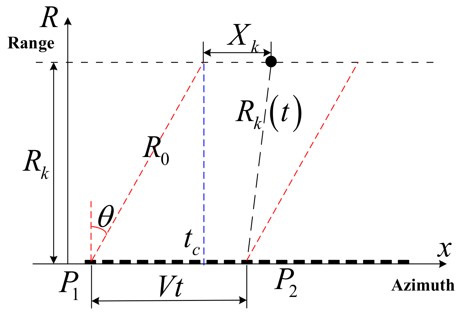
In this paper, the positive side view mode of spaceborne SAR is used for imaging. To construct an SAR imaging model, we usually use a single point target to represent the target in the scene, which is shown in Figure 1.
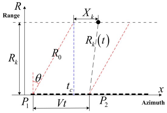
Figure 1.
Spaceborne SAR schematic diagram.
Assuming that the transmitted signal of the SAR platform is a linear frequency model (LFM) signal, the baseband echo signal received by the platform can be expressed as
where and are fast time and slow time, respectively. is the imaging scene area, is the scattering coefficient matrix of a scattering point in the scene, is the LFM signal, and is the squint distance between a scattering point and the SAR platform in a certain slow time. is the speed of light in vacuum and is the carrier frequency. denotes the complex Gaussian noise.
Furthermore, we can perform discrete sampling of the continuous-time echo signal, convert it into matrix , and discretize the scene scattering coefficient into matrix ; then, the following SAR observation model can be obtained from Equation (1):
where () is the vectorized echo matrix and () is the vectorized scene scattering coefficient matrix. is the observation matrix acquired from the discrete weight of (1), which contains the radar window function, SAR platform to target slope distance, echo phase, and other information. Here we refer to the existing research [5,6,7] and do not consider the phase matrix separately, because from the final imaging results, the amplitude information can already reflect the feasibility of the imaging algorithm.
For the underdetermined linear system in Equation (2), if the considered scene is sparse enough and the matrix meets the conditions of RIP [25,26], we can recover by solving the L1 optimization problem.
2.2. SAR Complex Signal Sparse Imaging Based on a Real-Value Model
When solving the SAR sparse imaging problem, prior information and optimization algorithms are used to estimate the scattering coefficient of multiple targets. Considering that SAR imaging problems are all realized in actual scenes, it is necessary to transform the SAR complex signal model into the corresponding real-value model. Therefore, Equation (2) is rewritten into the following real-value model
where , , , and denote the real parts of , , , and . Similarly, , , , and denote the imaginary parts of the respective matrix. Equation (3) is rewritten into the form of the corresponding real and imaginary system of equations
A complex observation model can be converted into a real-value model through the following relationship:
Equation (5) represents the real-value model of SAR sparse imaging. Next, imaging processing is only performed in the two-dimensional data domain instead of arranging two-dimensional echo data into vectors to continuously construct an observation matrix. The methods of traditional SAR sparse imaging references and Ref. [27] first vectorize the two-dimensional echo matrix and then design the imaging algorithm, which will inevitably cause an increase in the amount of calculation. When the imaging scene is large, the obtained vector dimension will become so high that it is difficult to obtain better imaging results. Therefore, its calculation cost is reduced to the same order of magnitude as the matched filter method, which makes sparse imaging of large-scale scenes possible.
2.3. Iterative Optimization of the Sparse Imaging Model Based on L1 Decoupling
For the SAR sparse real-value model in Section 2.2, we write the two-dimensional imaging model [26] as
where and denote the binary matrices to denote the downsampling strategy in azimuth and range directions, respectively. The matrix decomposition operation from Equations (5) and (6) is the Kronecker product. is Hadamard product operator. Furthermore, the dimension of the output result of this operation is still unchanged, but it has a very effective compression in terms of time and space complexity.
For the two-dimensional imaging model in Equation (6), the considered scene can be reconstructed by solving the L1 optimization problem
where denotes the Frobenius norm and is the regularization parameter, which controls the balance between data fidelity and sparsity.
However, it should be noted that due to the azimuth-distance coupling in the two-dimensional echo data domain, the observation matrix cannot be constructed directly [26], which means that based on the optimization problem in Equation (7), it is impossible to achieve sparse reconstruction of the considered scene.
In the implementation of the algorithm for reconstructing the signal, algorithms such as greedy algorithms or threshold iterations are generally used. In this paper, we use ISTA for signal reconstruction.
Generally, ISTA solves the reconstruction problem in Equation (7) by iterating between the following update steps:
where and denote the sparse and non-sparse estimations of , respectively. is an iterative parameter, denotes Frobenius norm, and is the residual.
However, ISTA usually requires multiple iterations to obtain satisfactory results and requires many calculations. The optimal transformation and related parameters are set based on prior information, but it is very difficult to obtain prior information in practice. Additionally, although we changed the original vectorization processing mode to two-dimensional matrix processing, the calculation still has a considerable burden. For example, it still takes more than 50s to reconstruct the targets in [26] experiments. We further consider the use of neural networks to learn some imaging parameters which can greatly reduce the amount of calculation in directly imaging.
3. SAR Deep Learning Imaging Method Based on ISTA
3.1. Construction of the Deep Learning Imaging Network
In recent years, data-driven methods based on deep learning have shown strong advantages in signal processing, especially in the field of image processing. As long as the network model is sufficiently complex, it can theoretically fit any nonlinear function [27]. Furthermore, any iterative algorithm can be expanded into the corresponding deep learning network structure. Considering that the essence of reconstructing the imaging model in Section 2 is to solve the nonlinear function problem, we naturally associate the problem of L1 iteration optimization with deep learning.
Equation (8) can be rewritten into the following form
where denotes the nonlinear activation function. and represent the weight and bias, respectively.
The single-layer network structure Equation (10) of is basically the same as that of the deep unfolding network [28], that is, the single-layer network with the same multilayer structure is stacked, and each layer can obtain the reconstruction results of the scattering coefficient.
At present, the sigmoid function, tanh function, and ReLU function are commonly used as deep learning activation functions [29]. Theoretically, any nonlinear activation function satisfying the condition can be used as the activation function of SAR learning imaging. Considering that the SAR imaging scene is likely to be sparse, a feasible scheme is to make the output value of the activation function as sparse as possible. Thus, we use the soft threshold function in ISTA as the activation function
where learnable parameter is .
Then, Equation (10) is expressed in the form of an operator update layer in the network
where the learnable parameter is .
Similarly, the activation function of the soft threshold function can be expressed as a nonlinear transformation layer Equation (11). Learnable parameters in the nonlinear transfer layer are nonlinear functions and regularization parameters . Of course, in addition to the existing neural network activation functions, adaptive activation functions related to the noise distribution of echo data and the prior distribution of scenes can also be designed. However, in SAR deep learning imaging, whether the activation function constructed by the prior distribution of echo data and scenes can satisfy the differentiability, monotonicity, and other activation function conditions need to be further studied [27]. The residual layer, operator update layer, and nonlinear transform layer constitute the single-layer topology of the SAR imaging network.
3.2. Training the Deep Learning Imaging Network
SAR deep learning imaging networks can be used for unsupervised training or supervised training [30] by using the known feature information of SAR target geometry size, shape, and statistical distribution. As the SAR imaging scene is unknown, it is impossible to directly use the scattering coefficient of the scene for error backpropagation.
To solve this problem, we use the scene scattering coefficient estimation obtained from the last layer of the network to multiply by the observation matrix to obtain the estimated SAR echo data, which can be compared with the original SAR echo data to realize the unsupervised training of the model.
In the process of unsupervised learning sample data, the method used in this paper is to downsample the original echo data, increase the system noise of different SNR, increase the echo phase disturbance, and so on, to realize the generation of unlabeled training samples. This method can not only reduce the quantity of data and increase imaging efficiency but also improve the robustness and reliability of the algorithm. The data downsampling method is shown in [6], which will not be repeated here. Considering the echo data defect in most practical application scenarios, in order to verify the imaging ability of SAR deep learning imaging method under this condition, downsampling is defined as the ratio of actual radar sampling points to sampling points according to Nyquist sampling rate.
Considering the increase in training noise for the system, for the SAR sparse imaging model, is the data fitting term, which reflects the fitting degree between the reconstructed signal and the original signal. As the noise we add is additive white noise to the system, we can use the Frobenius norm to express the data fitting term. To obtain a large number of training samples and ensure that the sparse imaging model of SAR is not changed, different Gaussian white noise can be added to the original echo data.
Furthermore, the primary phase disturbance and secondary phase disturbance with different amplitudes can be added to the SAR echo phase to realize the sample generation of echo data. The phase disturbance simulates the motion compensation error of the SAR platform, which can be used to verify the robustness of the deep learning network to imaging phase error. Assume that the sample database is a and N is the number of samples. If the mean square error loss function is used, the cost function can be written as
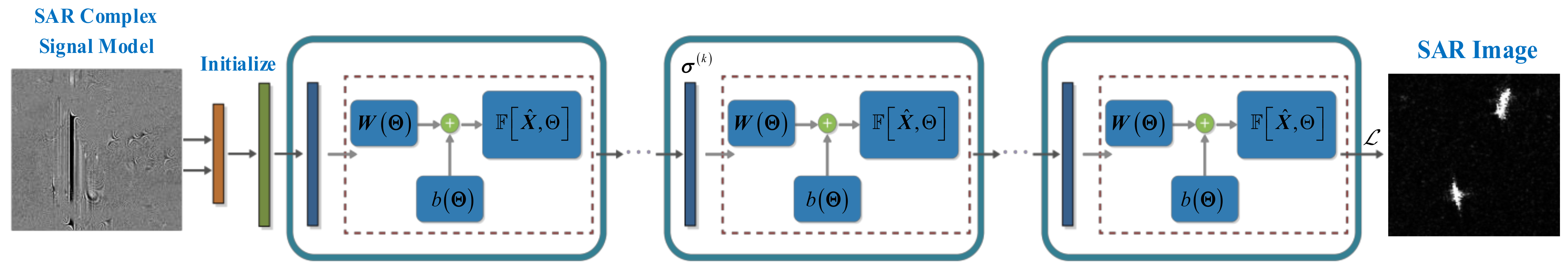
The advantage of unsupervised training is that there is no need to add any label to SAR data, which greatly reduces the training cost of the SAR learning imaging network. The overall framework of our proposed method is given in Figure 2.
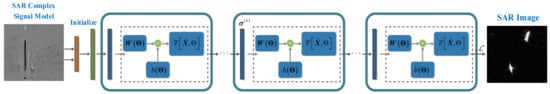
Figure 2.
Overall framework of the proposed SAR deep learning imaging method.
4. Experiments and Analysis
To test the feasibility of the proposed deep learning SAR sparse imaging algorithm, we use the simulated data and measured data to verify jointly. Among them, the simulated data consist of nine different scattering points on the surface. The measured data include vehicles, ships, and planes in different scenes, which are from the MSTAR and Gaofen-3 datasets. To verify the superiority of the proposed algorithm, deep learning SAR sparse imaging is compared with the existing imaging algorithms ISTA [5] and fast ISTA [6].
The radar parameters used in this paper are shown in Table 1. For unification, we uniformly consider the polarization mode of SAR as VH in the experiment. To highlight the reliability of the algorithm, the downsampling of the echo data is directly adopted during imaging processing.

Table 1.
Parameters of radar.
4.1. Simulation Point Target Imaging Experiment
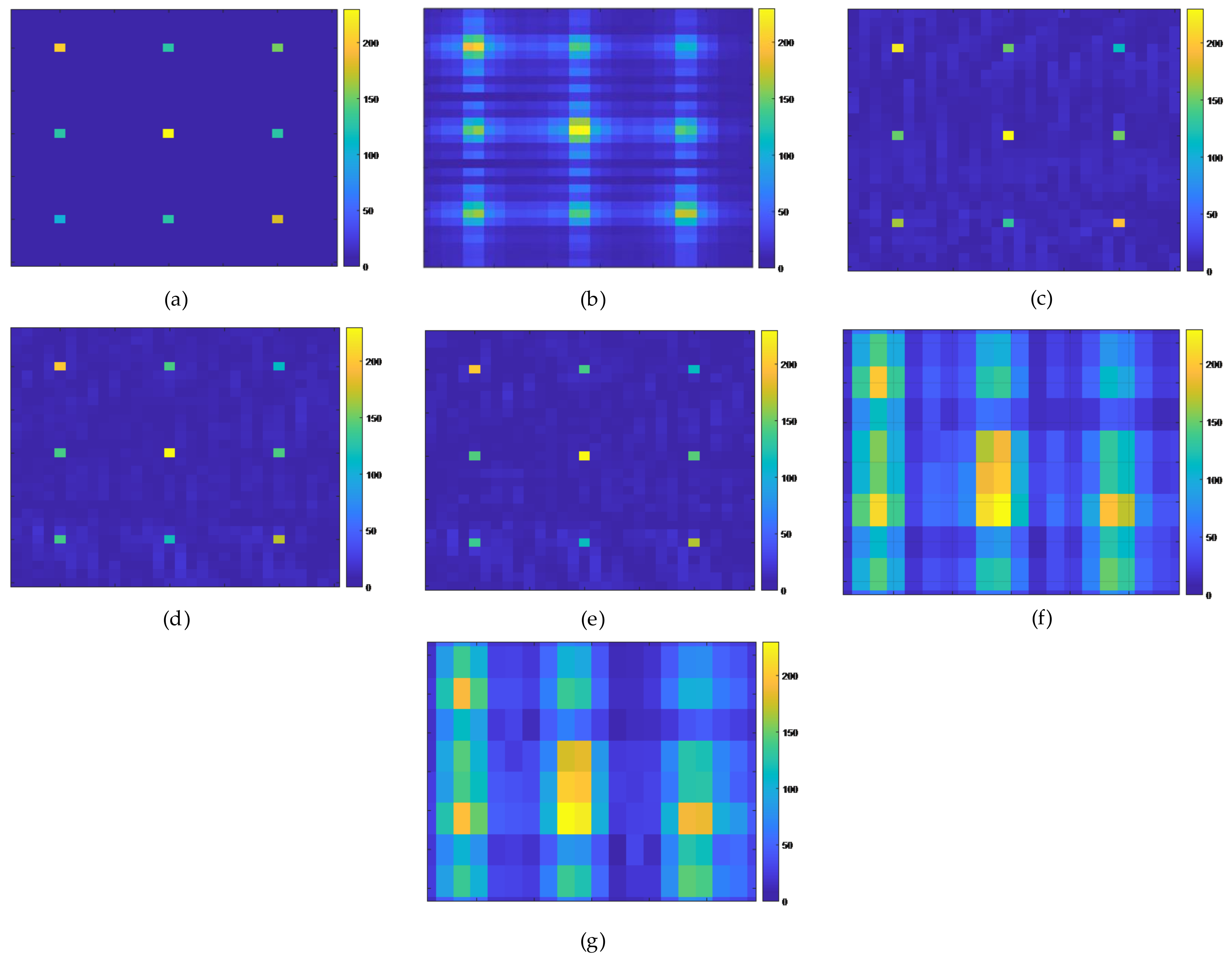
In this section, the SAR imaging model in the presence of Gaussian white noise is taken as the simulation object. The input SNR of the echo is set to 20 dB. The imaging region is discretized into a 30 × 30 grid scene, which contains nine scattering points with different scattering coefficients. In terms of network parameters, the initial learning rate is 0.0001, the epoch number is 100, and the layer number is set to L. In actual imaging, the trained imaging observation matrix, regularization parameters, iteration step length, and other parameters are directly input into the imaging network, and the imaging results are output after forward propagation through the network. The simulated data imaging needs to be compared with the original SAR echo data, so the network training is first performed under the full sampling data structure. The quantity of data for the training to be imaged by no more than five scattering points is 1000. The results of the comparative experiment are shown in Figure 3.
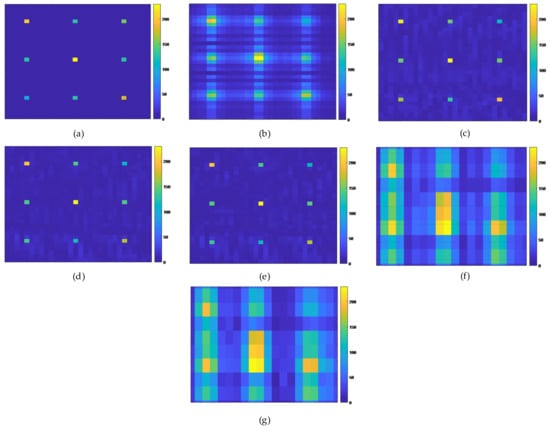
Figure 3.
Point target imaging results. (a) is original point target, (b) is Range Doppler method, (c) is our proposed method with L = 3, (d) is our proposed method with L = 8, (e) is our proposed method with L = 11, (f) is ISTA method and (g) is Fast ISTA method.
It can be seen in the imaging results in Figure 3 that under the premise of downsampling the echo data, our proposed method and the two ISTA imaging algorithms have a large imaging quality degradation. We also show the imaging results of the traditional Range Doppler method [31] under downsampling condition in Figure 3b, which also has much side lobe interference. Since the scattering points have short distance and the scattering coefficients are relatively close, the imaging results inevitably reveal side lobes and other clutter interference. For the proposed method, the loss of unsupervised training is compared with the original echo data by using the estimated echo data. Therefore, when a large quantity of original data is lost, the imaging quality of unsupervised training methods cannot be further improved.
Although all methods can correctly reconstruct the coordinate position of the point target, it is obvious that the superiority of our proposed method in reconstruction can be seen. Both ISTA and fast ISTA have a large degree of defocus, and the imaging quality is significantly worse than that of our proposed method. Compared with the imaging results at L = 3, the imaging results at L = 8 and L = 11 are obviously better at suppressing side lobes. However, the imaging result of L = 11 is not too far from the result of L = 8, which shows that we can use fewer network layers to achieve simulation point target imaging. After comparing the imaging results, we also counted the comparison results of the peak signal-to-noise ratio (PSNR), mean square error (NMSE), peak sidelobe ratio (PLSR), and imaging time of the three methods. Table 2 shows the comparison results.
Table 2.
Comparison of imaging quality and imaging time.
The experimental results given in Table 2 can also reflect the experimental results of Figure 3, and the proposed method obtains the imaging results of thousands of iterations better than the existing mainstream iteration optimization algorithm by using a small number of network layers under the condition of unsupervised training. In terms of imaging speed, after the imaging network has trained the network parameters, the imaging process only requires forward feeding, and the number of network layers is small, so the imaging speed is faster than the ISTA and fast ISTA for multiple iterations.
4.2. Measured Target Imaging Experiment
In this section, the effectiveness of the proposed method is further verified by using measured SAR data from the MSTAR and Gaofen-3 satellites. The imaging algorithms used to obtain the MSTAR and Gaofen-3 datasets are traditional Range Doppler, Chirp Scaling, etc. The selected measured SAR data include the following three observation scenes: (a) ground observation scene, which contains a single-vehicle target, (b) sea surface observation scene, which contains several ship targets, and (c) ground airport observation scene, which contains multiple planes. In fact, several other vehicle targets in this dataset can be used as our experimental objects, and here are just these two vehicle targets (T72 and ZSU-23–4) selected for experimental demonstration. For the measured data, the position relationship between the imaging scene of the simulated echo data and the radar is consistent with the previous point target simulation experiment, and the phase information of the echo data can be obtained by a two-dimensional Fourier transform of the complex image data. The network parameters are the same as in the previous section, and no training is performed on the measured data. The imaging results are shown in Figure 4, Figure 5, Figure 6, Figure 7, Figure 8 and Figure 9.
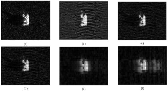
Figure 4.
T72 imaging results. (a) is original vehicle target, (b) is our proposed method with L = 3, (c) is our proposed method with L = 8, (d) is our proposed method with L = 11, (e) is ISTA method and (f) is Fast ISTA method.
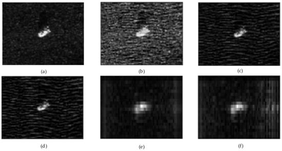
Figure 5.
ZSU-23–4 imaging results. (a) is original vehicle target, (b) is our proposed method with L = 3, (c) is our proposed method with L = 8, (d) is our proposed method with L = 11, (e) is ISTA method and (f) is Fast ISTA method.
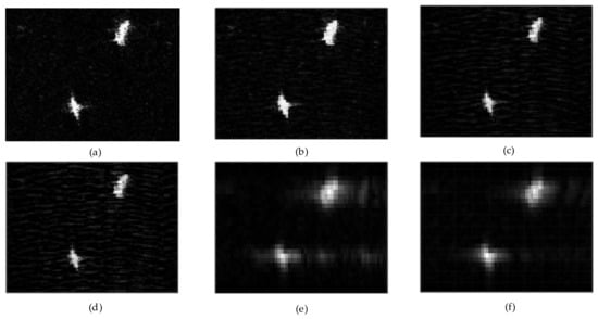
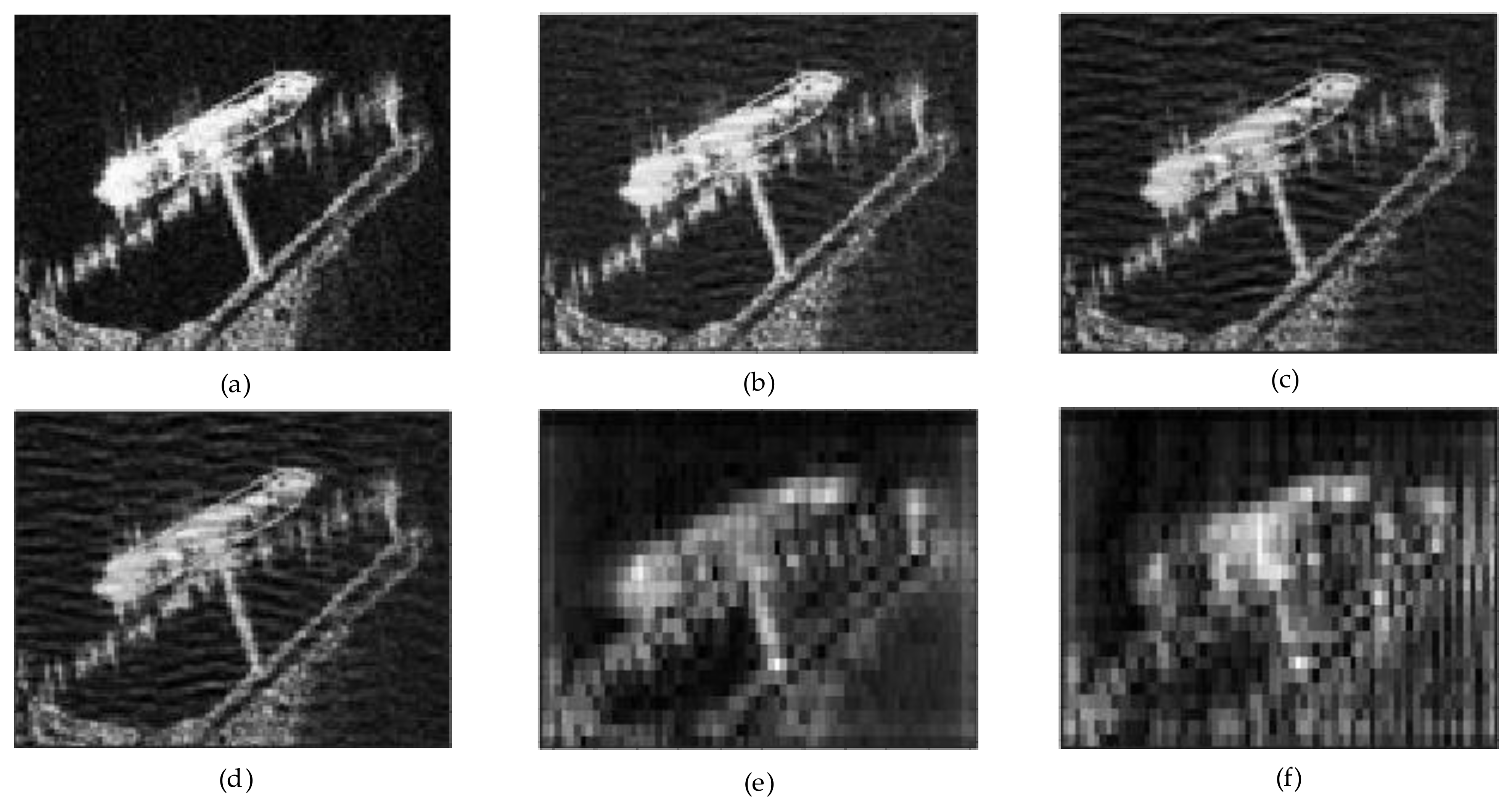
Figure 6.
Ship targets on the sea imaging results. (a) is original ship target, (b) is our proposed method with L = 3, (c) is our proposed method with L = 8, (d) is our proposed method with L = 11, (e) is ISTA method and (f) is Fast ISTA method.
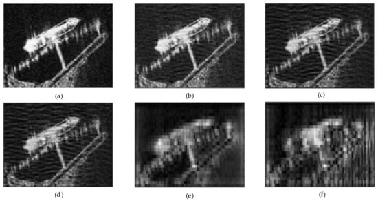
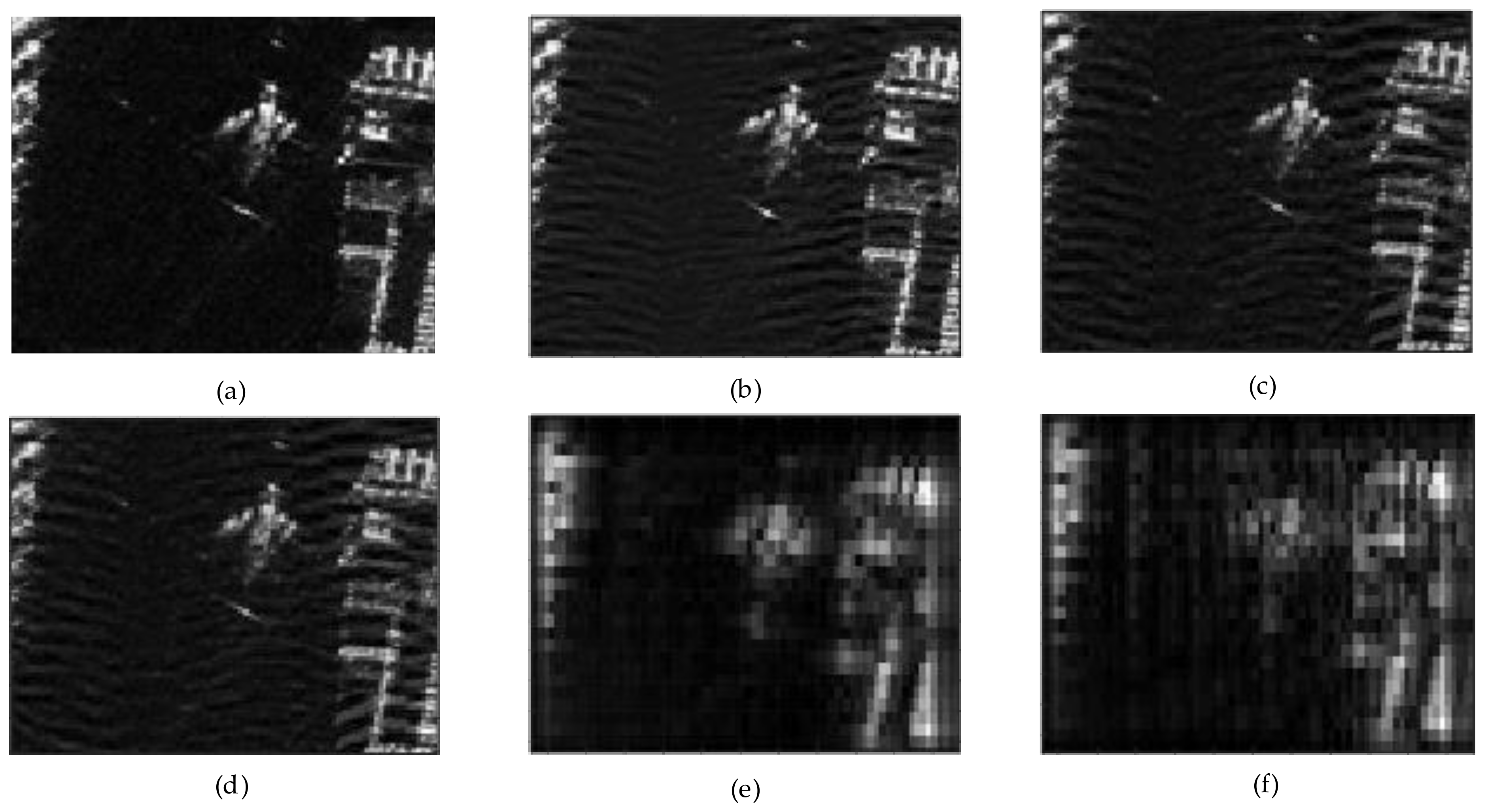
Figure 7.
Inshore ship target imaging results. (a) is original ship target, (b) is our proposed method with L = 3, (c) is our proposed method with L = 8, (d) is our proposed method with L = 11, (e) is ISTA method and (f) is Fast ISTA method.
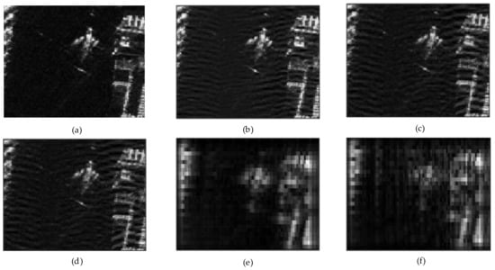
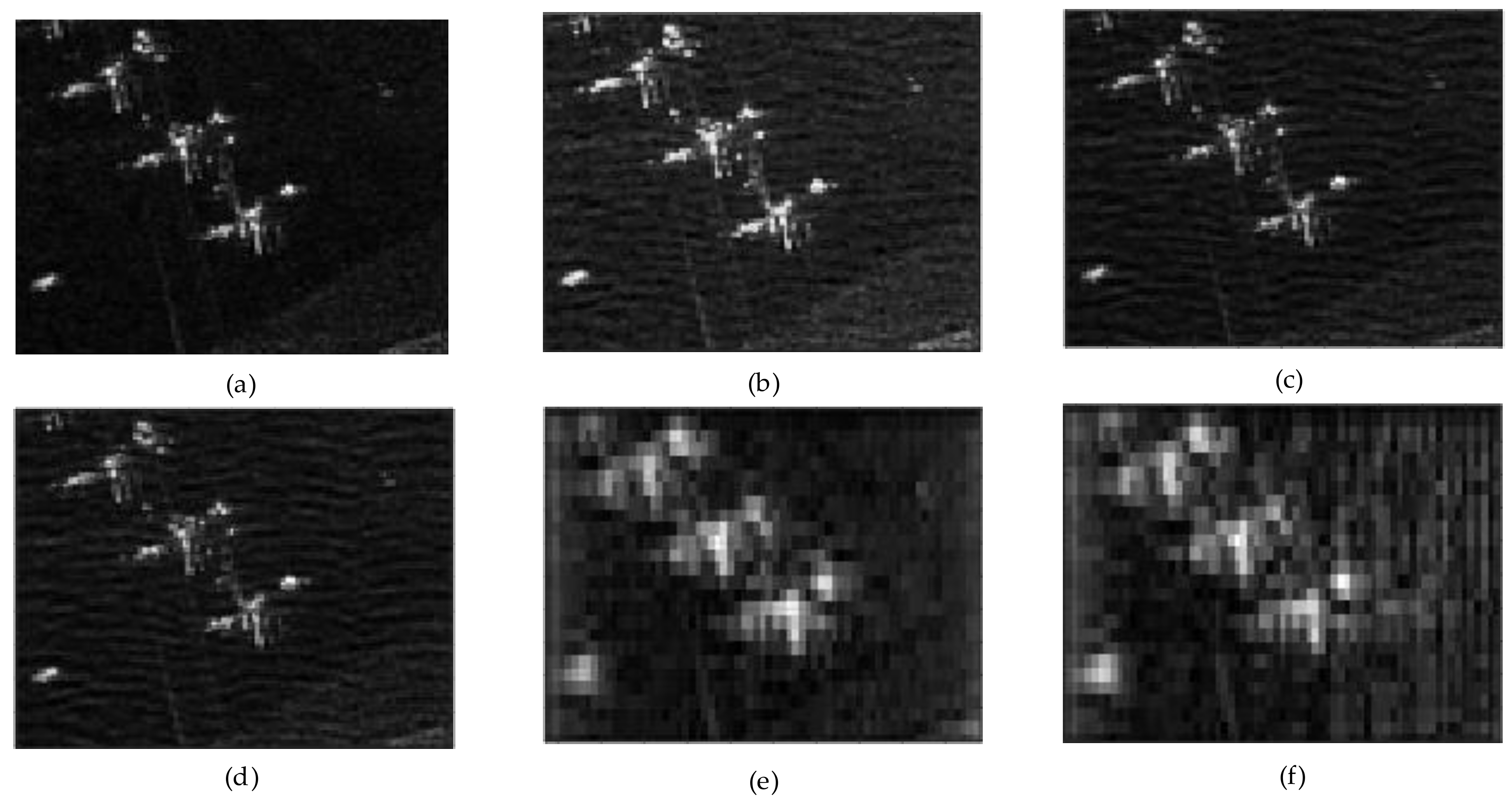
Figure 8.
Plane target imaging results. (a) is original plane target, (b) is our proposed method with L = 3, (c) is our proposed method with L = 8, (d) is our proposed method with L = 11, (e) is ISTA method and (f) is Fast ISTA method.

Figure 9.
Plane target imaging results. (a) is original plane target, (b) is our proposed method with L = 3, (c) is our proposed method with L = 8, (d) is our proposed method with L = 11, (e) is ISTA method and (f) is Fast ISTA method.
It can be seen in Figure 4, Figure 5, Figure 6, Figure 7, Figure 8 and Figure 9 that under the condition of downsampling, the imaging algorithm we proposed is still better than the two iterative optimization algorithms.
We selected T72 and ZSU-23–4 in the MSTAR dataset as the imaging objects. For the single vehicle target, because of the large downsampling rate, both the ISTA and fast ISTA algorithms have different degrees of defocusing. However, the methods we proposed can achieve better reconstruction results. In contrast, the refocusing effect for vehicle targets and the effect of background clutter suppression are also better when L = 8. The possible reason is that when L = 3, all the parameters in the imaging model are not fully learned; and when L = 11, over-fitting of the network occurs. For imaging the ship targets on the sea, we selected two offshore ship targets and one inshore ship target. Figure 6 shows that the three methods can be accurately implemented for imaging on relatively sparse sea scenes. This situation is similar to the imaging results of the single vehicle target. On the offshore scene, due to the sparse background, our imaging algorithm can achieve better reconstruction and suppress clutter interference. For inshore scenes, the image quality of ISTA and Fast ISTA is poor, because the inshore scenes contain a wide variety of targets. Containers and bridges on shore all have high scattering coefficients, causing great interference in the accurate reconstruction of ship targets. However, for the inshore ship, Figure 7 shows that our method achieves a better imaging result which means our proposed method can reconstruct the target better in a complex background. Figure 8 and Figure 9 also show the imaging results in the airport scene. The airport scene is also a challenging task for imaging because the airport scene is more complex with irregular arrangement of a variety of buildings and planes may be densely distributed. In Figure 8, our proposed method reconstructs the plane and the building next to it integrally, while ISTA and Fast ISTA cannot distinguish the plane and other targets. When three planes are parked close together in Figure 9, the scattering points interfere with the imaging. Experimental results show that our method can also reconstruct such densely distributed targets.
Therefore, SAR images obtained by the proposed imaging network have higher reconstruction accuracy, and the target scenes are better preserved, and the background clutter is further suppressed. Since we do not change the parameters of the network, PSNR, NMSE, and PLSR in the measured data part are almost the same as the results in the simulation data given in Table 2. Due to the different scenes of the imaging targets, the imaging time of the measured data is shown in Table 3.
Table 3.
Comparison of imaging time.
5. Conclusions
In this paper, an end-to-end SAR deep learning imaging method based on a sparse optimization iterative algorithm was proposed. Referring to the existing SAR sparse imaging algorithm, the SAR imaging model was first rewritten into an SAR complex signal form based on the real-value model. Next, because of the deep learning imaging algorithm based on sparse optimization, the above model was further written into a sparse imaging model based on L1 decoupling. Then, the deep learning imaging network was established based on the two-dimensional SAR observation model, the solution process of the two-dimensional model was mapped to a layer of the neural network, and the scene scattering coefficient was solved through the stacking and expansion of the multilayer network. The original fixed imaging model parameters were changed into learnable network parameters. Through unsupervised training, the network independently learns to obtain the model parameters with the best imaging quality and improve the universality and generalization ability of the imaging method to SAR echo data. Finally, the proposed algorithm was verified in both the simulated point echo data and the measured target data with different targets in multiple scenes, which proves the feasibility and reliability of the method.
Moreover, the disadvantages of unsupervised training are also obvious. First, there are certain requirements for the sampling rate and SNR of radar echo. When the sampling rate is insufficient or the echo is compressed, the quantity of echo data is greatly reduced, thus affecting the accuracy of the cost function. Second, the prior information and known characteristics of the target in the scene are ignored, which cannot further improve the imaging performance of the key target. Therefore, in future research, we will focus more on how to further improve the imaging effect and supervise deep learning imaging algorithms. Simultaneously, how to make the reconstructed image have complete information of the phase and background statistical distribution so that the images obtained by these algorithms can better support some important SAR applications has also become a focus of our follow-up research.
Author Contributions
Conceptualization, S.Z. and J.N.; methodology, S.Z.; software, S.Z. and S.X.; validation, S.Z., S.X. and J.L.; formal analysis, J.L.; investigation, S.Z.; resources, J.N.; data curation, S.Z. and Y.L.; writing—original draft preparation, S.Z. and J.L.; writing—review and editing, S.Z.; visualization, S.Z.; supervision, J.L. and Y.L.; project administration, Y.L.; funding acquisition, J.N. and Y.L. All authors have read and agreed to the published version of the manuscript.
Funding
This research is funded by The National Natural Science Foundation of China, grant number 62131020, 62001508 and 61871396, and Natural Science Basic Research Program of Shaanxi, grant number 2020JQ-480.
Institutional Review Board Statement
Not applicable.
Informed Consent Statement
Not applicable.
Data Availability Statement
Not applicable.
Conflicts of Interest
The authors declare no conflict of interest.
References
- Zhou, F.; Zhao, B.; Tao, M.; Bai, X.; Chen, B.; Sun, G. A large scene deceptive jamming method for space-borne SAR. IEEE Trans. Geosci. Remote Sens. 2013, 51, 4486–4495. [Google Scholar] [CrossRef]
- Xu, Z.; Zhang, B.; Zhou, G.; Zhong, L.; Wu, Y. Sparse SAR Imaging and Quantitative Evaluation Based on Nonconvex and TV Regularization. Remote Sens. 2021, 13, 1643. [Google Scholar] [CrossRef]
- Yang, W.; Chen, J.; Liu, W.; Wang, P.B.; Li, C.S. A Modified Three-Step Algorithm for TOPS and Sliding Spotlight SAR Data Processing. IEEE Trans. Geosci. Remote Sens. 2017, 55, 6910–6921. [Google Scholar] [CrossRef] [Green Version]
- Ni, J.C.; Zhang, Q.; Luo, Y.; Sun, L. Compressed sensing SAR imaging based on centralized sparse representation. IEEE Sens. J. 2018, 18, 4920–4933. [Google Scholar] [CrossRef]
- Bi, H.; Li, Y.; Zhu, D.Y.; Bi, B.A.; Zhang, B.C.; Hong, W.; Wu, Y.R. An improved iterative thresholding algorithm for L1-norm regularization based sparse SAR imaging. Sci. China Inf. Sci. 2020, 63, 219301:1–219301:3. [Google Scholar] [CrossRef]
- Fang, J.; Xu, Z.B.; Zhang, B.C.; Hong, W.; Wu, Y.R. Fast Compressed Sensing SAR Imaging Based on Approximated Observation. IEEE J. Sel. Top. Appl. Earth Obs. Remote Sens. 2014, 7, 352–363. [Google Scholar] [CrossRef] [Green Version]
- Shi, W.; Jiang, F.; Zhang, S.; Zhao, D. Deep networks for compressed image sensing. In Proceedings of the 2017 IEEE International Conference on Multimedia and Expo (ICME), Hong Kong, China, 10–14 July 2017; pp. 877–882. [Google Scholar] [CrossRef] [Green Version]
- Zhang, J.; Ghanem, B. ISTA-Net: Interpretable Optimization-Inspired Deep Network for Image Compressive Sensing. In Proceedings of the 2018 IEEE/CVF Conference on Computer Vision and Pattern Recognition, Salt Lake City, UT, USA, 18–23 June 2018; pp. 1828–1837. [Google Scholar] [CrossRef] [Green Version]
- Zhang, Y.; Mu, H.L.; Xiao, T.; Jiang, Y.C.; Ding, C. SAR imaging of multiple maritime moving targets based on sparsity Bayesian learning. IET Radar Sonar Navig. 2020, 14, 1717–1725. [Google Scholar] [CrossRef]
- Ma, T.; Li, H.; Yang, H.; Lv, X.L.; Li, P.Y.; Liu, T.J.; Yao, D.Z.; Xu, P. The extraction of motion-onset VEP BCI features based on deep learning and compressed sensing. J. Neurosci. Methods 2017, 275, 80–92. [Google Scholar] [CrossRef] [PubMed]
- Liang, P.Z.; Fan, J.C.; Shen, W.H.; Qin, Z.J.; Li, G.Y. Deep Learning and Compressive Sensing-Based CSI Feedback in FDD Massive MIMO Systems. IEEE Trans. Veh. Technol. 2020, 69, 9217–9222. [Google Scholar] [CrossRef]
- Ma, W.Y.; Qi, C.H.; Zhang, Z.C.; Cheng, J.L. Sparse Channel Estimation and Hybrid Precoding Using Deep Learning for Millimeter Wave Massive MIMO. IEEE Trans. Commun. 2020, 68, 2838–2849. [Google Scholar] [CrossRef] [Green Version]
- Cao, X.H.; Ji, Y.M.; Wang, L.; Ji, B.B.; Jiao, L.C.; Han, J.G. SAR image change detection based on deep denoising and CNN. IET Images Process. 2019, 13, 1509–1515. [Google Scholar] [CrossRef]
- Zhou, Y.Y.; Shi, J.; Wang, C.; Hu, Y.; Zhou, Z.N.; Yang, X.Q.; Zhang, X.L.; Wei, S.J. SAR Ground Moving Target Refocusing by Combining mRe3 Network and TVβ-LSTM. IEEE Trans. Geosci. Remote Sens. 2020, 1–14. [Google Scholar] [CrossRef]
- Shi, H.Y.; Lin, Y.; Guo, J.W.; Liu, M.X. ISAR autofocus imaging algorithm for maneuvering targets based on deep learning and keystone transform. J. Syst. Eng. Electron. 2020, 31, 1178–1185. [Google Scholar]
- Shi, W.Z.; Jiang, F.; Liu, S.H.; Zhao, D.B. Image Compressed Sensing Using Convolutional Neural Network. IEEE Trans. Image Process. 2020, 29, 375–388. [Google Scholar] [CrossRef]
- Qin, R.; Fu, X.J.; Dong, J.; Jiang, W. A semi-greedy neural network CAE-HL-CNN for SAR target recognition with limited training data. Int. J. Remote Sens. 2020, 41, 7889–7911. [Google Scholar] [CrossRef]
- Merhej, D.; Diab, C.; Khalil, M.; Prost, R. Embedding Prior Knowledge Within Compressed Sensing by Neural Networks. IEEE Trans. Neural Netw. 2011, 22, 1638–1649. [Google Scholar] [CrossRef] [PubMed]
- Bu, H.X.; Tao, R.; Bai, X.; Zhao, J. A Novel SAR Imaging Algorithm Based on Compressed Sensing. IEEE Geosci. Remote Sens. Lett. 2015, 12, 1003–1007. [Google Scholar] [CrossRef]
- Kang, M.S.; Kim, K.T. Ground Moving Target Imaging Based on Compressive Sensing Framework with Single-Channel SAR. IEEE Sens. J. 2020, 20, 1238–1250. [Google Scholar] [CrossRef]
- Jung, S.; Cho, Y.; Park, R.; Kim, J.; Jung, H.; Chung, Y. High-Resolution Millimeter-Wave Ground-Based SAR Imaging via Compressed Sensing. IEEE Trans. Magn. 2018, 54, 9400504. [Google Scholar] [CrossRef]
- Kang, M.S.; Kim, K.T. Compressive Sensing Based SAR Imaging and Autofocus Using Improved Tikhonov Regularization. IEEE Sens. J. 2019, 19, 5529–5540. [Google Scholar] [CrossRef]
- Khwaja, A.S.; Ma, J.W. Applications of Compressed Sensing for SAR Moving-Target Velocity Estimation and Image Compression. IEEE Trans. Instrum. Meas. 2011, 60, 2848–2860. [Google Scholar] [CrossRef]
- Hou, B.; Wei, Q.; Zheng, Y.; Wang, S. Unsupervised Change Detection in SAR Image Based on Gauss-Log Ratio Image Fusion and Compressed Projection. IEEE J. Sel. Top. Appl. Earth Obs. Remote Sens. 2014, 7, 3297–3317. [Google Scholar] [CrossRef]
- Candés, E.J.; Romberg, J.K.; Tao, T. Stable signal recovery from incomplete and inaccurate measurements. Commun. Pure Appl. Math. 2006, 59, 1207–1223. [Google Scholar] [CrossRef] [Green Version]
- Bi, H.; Bi, G.A.; Zhang, B.C.; Hong, W. Complex-Image-Based Sparse SAR Imaging and Its Equivalence. IEEE Trans. Geosci. Remote Sens. 2018, 56, 5006–5014. [Google Scholar] [CrossRef]
- Luo, Y.; Ni, J.C.; Zhang, Q. Synthetic aperture radar learning-imaging method based on data-driven technique and artificial intelligence. J. Radars 2020, 9, 107–122. [Google Scholar]
- Borgerding, M.; Schniter, P.; Rangan, S. AMP inspired deep networks for sparse linear inverse problems. IEEE Trans. Signal Process. 2017, 65, 4293–4308. [Google Scholar] [CrossRef]
- Ye, G.Y.; Zhang, Z.X.; Ding, L.; Li, Y.W.; Zhu, Y.M. GAN-Based Focusing-Enhancement Method for Monochromatic Synthetic Aperture Imaging. IEEE Sens. J. 2020, 20, 11484–11489. [Google Scholar] [CrossRef]
- Lu, Z.J.; Qin, Q.; Shi, H.Y.; Huang, H. SAR moving target imaging based on convolutional neural network. Digit. Signal Process. 2020, 106, 102832. [Google Scholar] [CrossRef]
- Zhang, J.; Pei, Z. Ground-based SAR imaging based on improved Range-Doppler algorithm. In Proceedings of the International Radar Conference IET, Xi’an, China, 14–16 April 2013. [Google Scholar]


Publisher’s Note: MDPI stays neutral with regard to jurisdictional claims in published maps and institutional affiliations. |
© 2021 by the authors. Licensee MDPI, Basel, Switzerland. This article is an open access article distributed under the terms and conditions of the Creative Commons Attribution (CC BY) license (https://creativecommons.org/licenses/by/4.0/).