
Rotation-Invariant and Relation-Aware Cross-Domain Adaptation Object Detection Network for Optical Remote Sensing Images


Abstract
: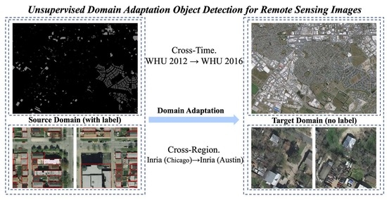
1. Introduction
- We propose a novel algorithm framework to solve the problem of unsupervised CDAOD in remote sensing images. The highest accuracy is achieved in three building detection adaptation scenarios with obvious domain shift.
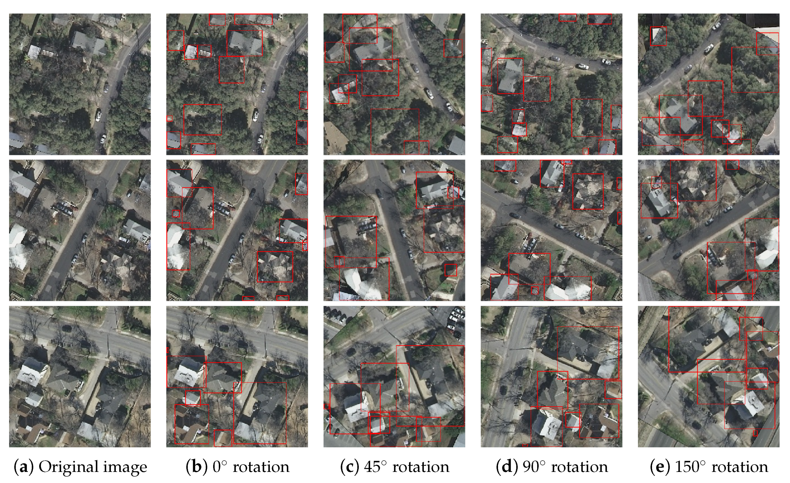
- We propose to use the rotation-invariant regularizer term in both the source domain and the target domain to solve the problem of direction arbitrariness in remote sensing images.
- To aggregate regional information, a prototype-level domain alignment based on relation-aware graph is proposed to make the instance information obtained by the detection network more accurate.
2. Related Work
2.1. Cross-Domain Object Detection in the Computer Vision Field
2.2. Cross-Domain Object Detection in the Remote Sensing Field
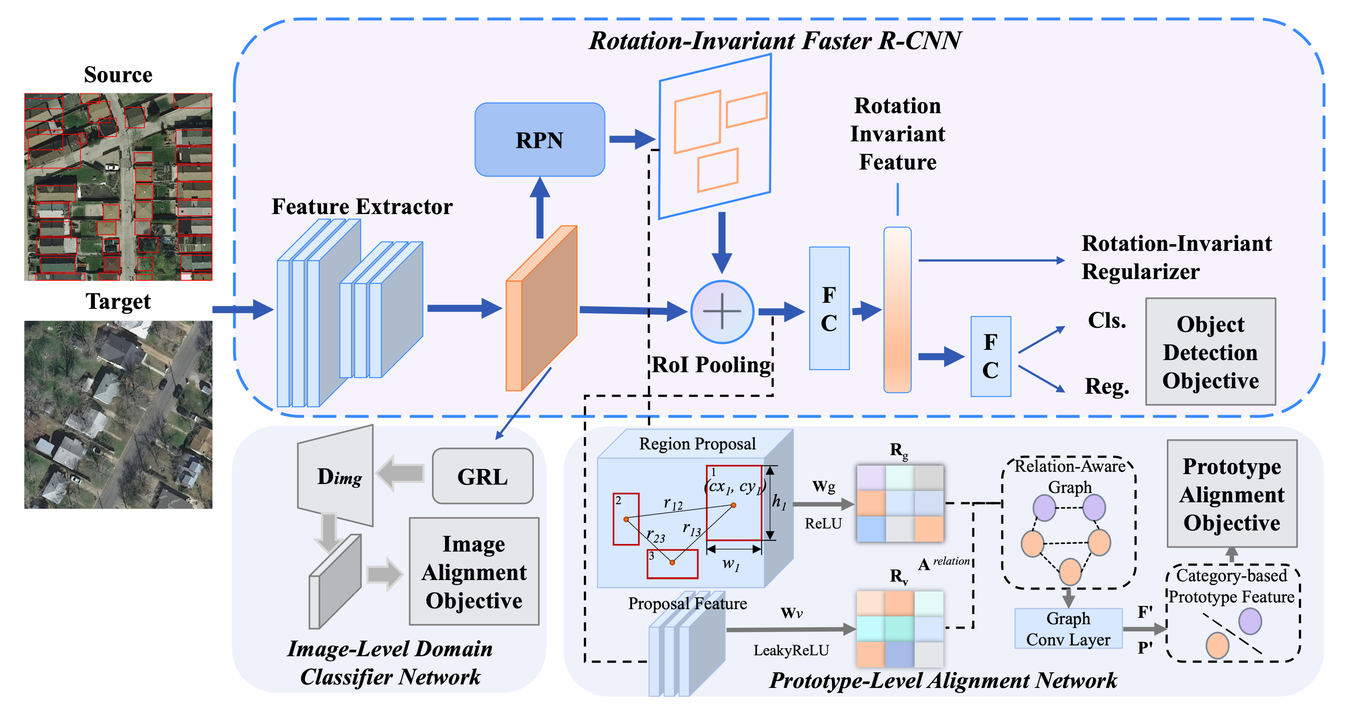
3. Methodology
3.1. Rotation-Invariant Regularizer
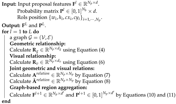
3.2. Prototype-Level Alignment Based on Relation-Aware Graph
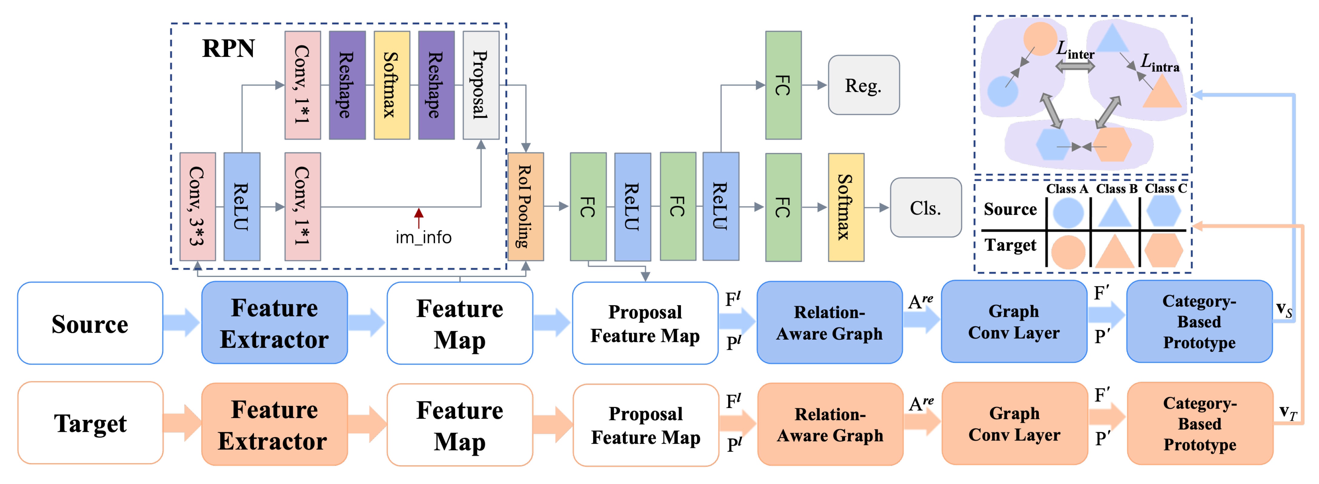
3.2.1. Region Proposal Generation
3.2.2. Constructing Relation-Aware Graph
3.2.3. Graph-Based Region Aggregation
3.2.4. Generating Prototype Features
| Algorithm 1: Relation-Aware Graph Convolutional Layer. The number of the layer is L. Geometric transformation matrix: . Visual transformation matrix: . The number of RoIs is . Layer transformation matrix: . |
 |
3.2.5. Category-Level Domain Alignment
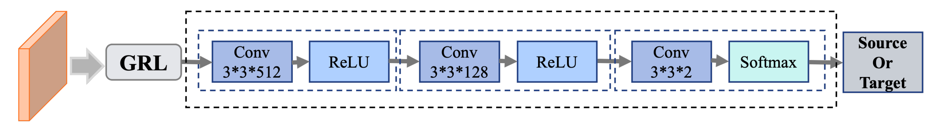
3.3. Image-Level Domain Alignment
3.4. Overall Training Objective
4. Experiments and Results
4.1. Datasets
4.2. Evaluation Metrics
4.3. Implementation Details
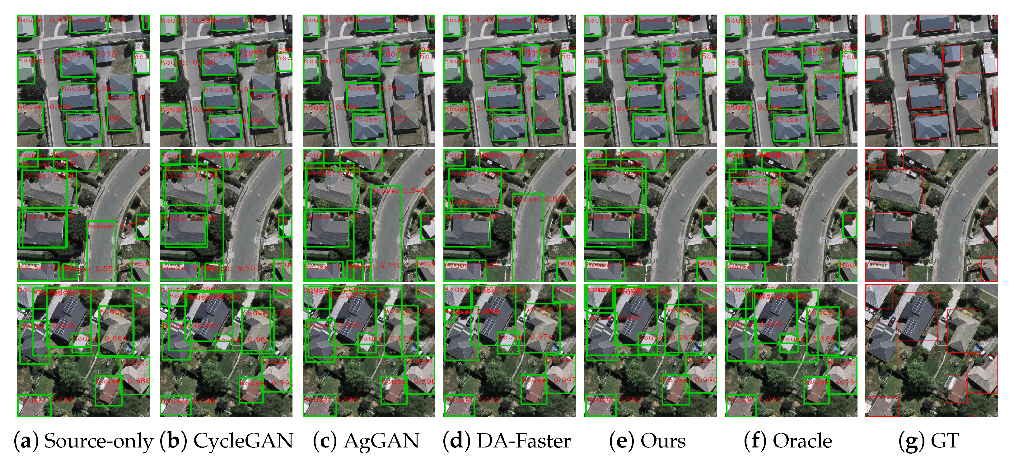
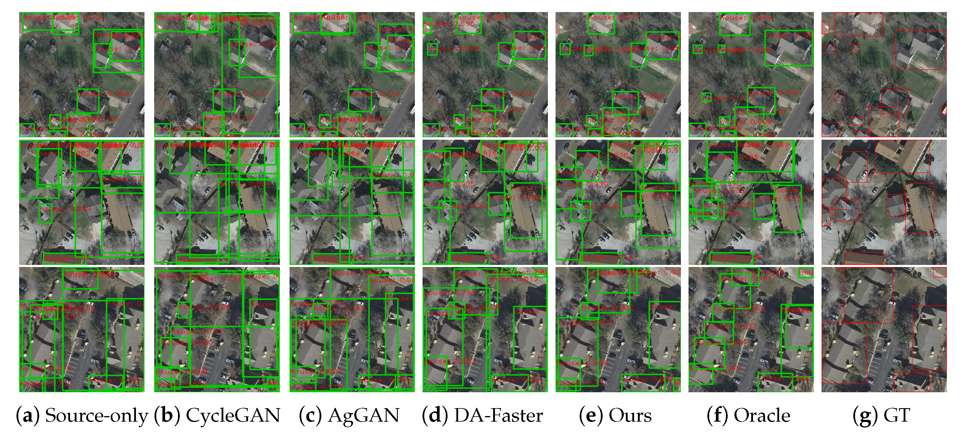
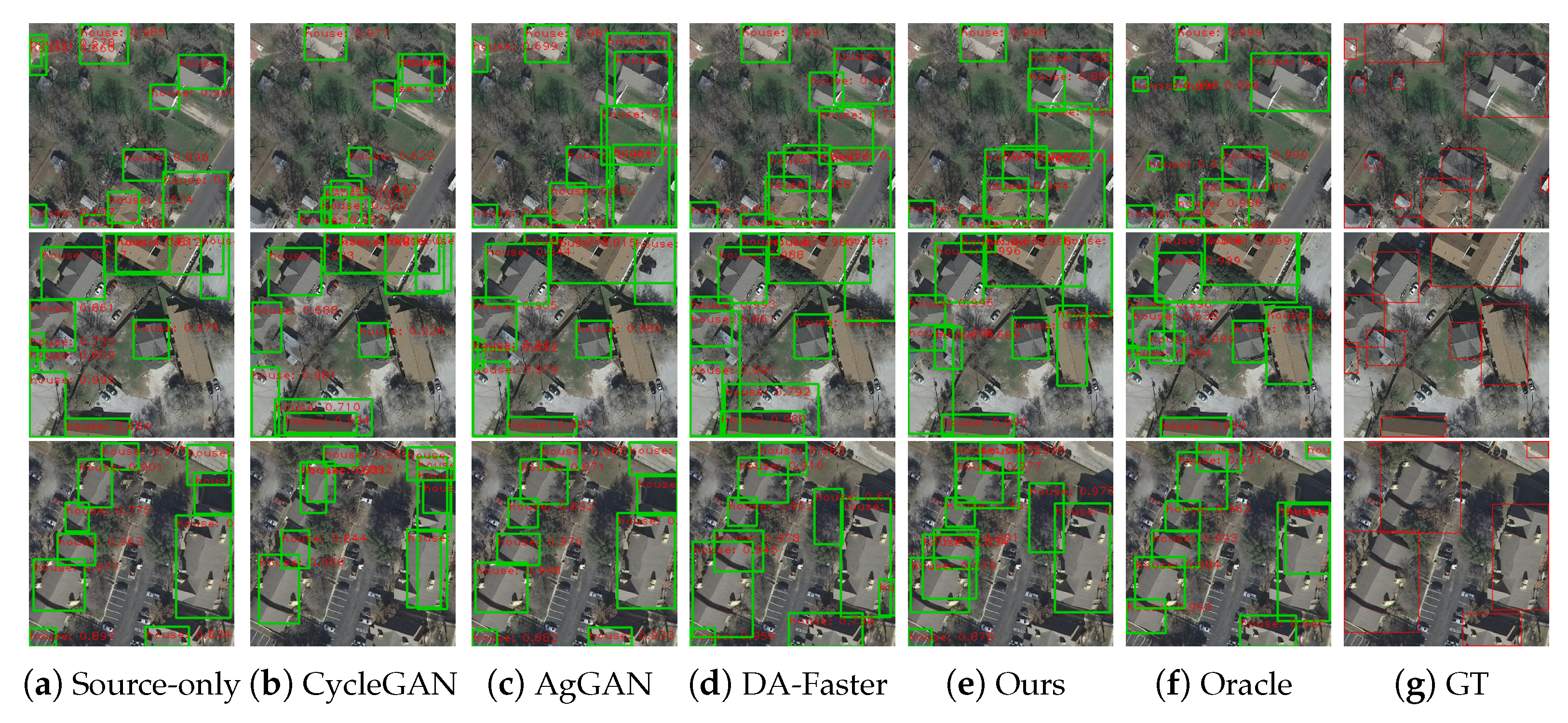
4.4. Results
- (1)
- , same data source and region, different times;
- (2)
- , same data source, different regions;
- (3)
- , different data source, different regions.
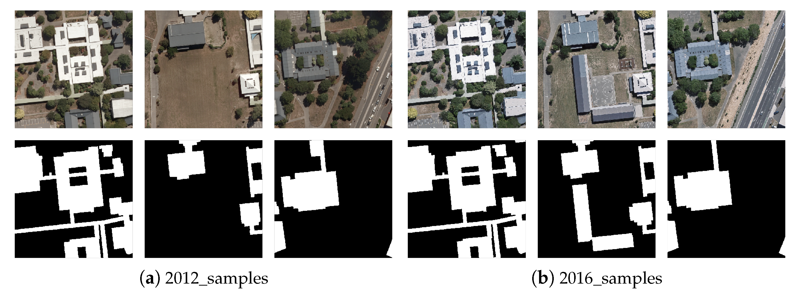
4.4.1. Cross-Time. WHU 2012 → WHU 2016
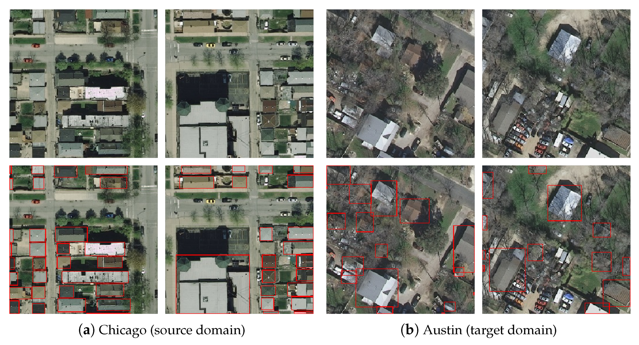
4.4.2. Cross-Region. Inria (Chicago) → Inria (Austin)
4.4.3. Cross Data Source and Cross-Region. WHU 2012 → Inria (Austin)
5. Discussion
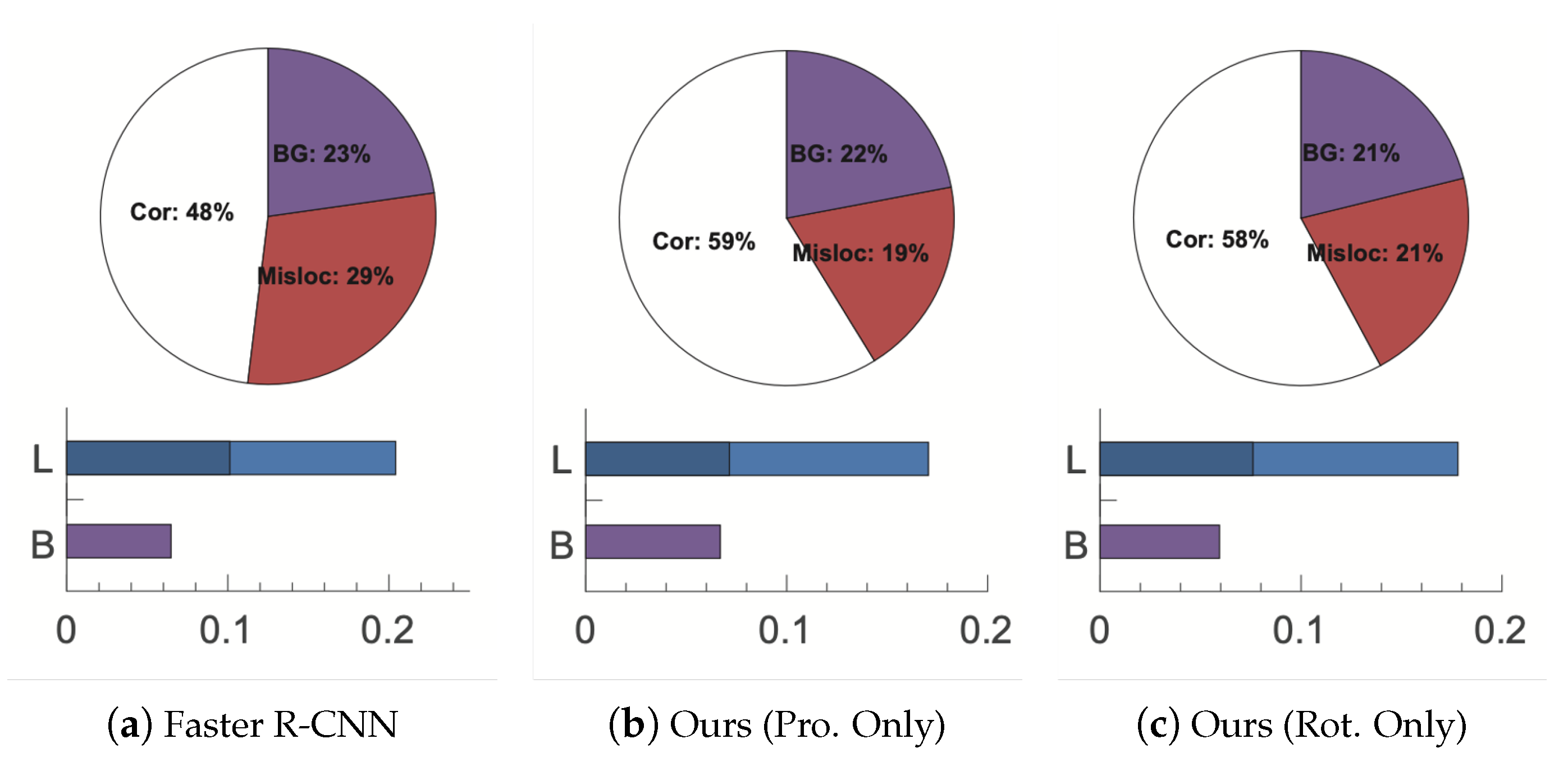
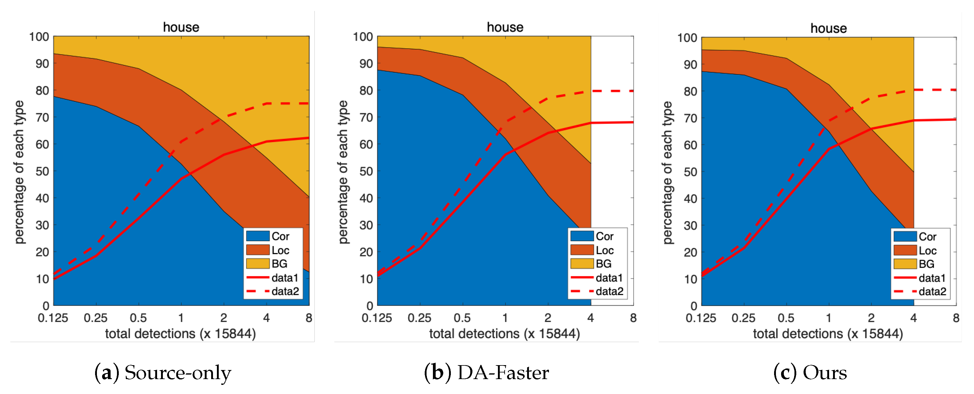
5.1. Performance Analysis Focusing on Errors
5.2. Analysis of P–R Curve
5.3. Parameter Sensitivity
6. Conclusions
Author Contributions
Funding
Data Availability Statement
Acknowledgments
Conflicts of Interest
References
- Lecun, Y.; Bottou, L.; Bengio, Y.; Haffner, P. Gradient-based learning applied to document recognition. Proc. IEEE 1998, 86, 2278–2324. [Google Scholar] [CrossRef] [Green Version]
- Krizhevsky, A.; Sutskever, I.; Hinton, G.E. ImageNet Classification with Deep Convolutional Neural Networks. Commun. ACM 2017, 60, 84–90. [Google Scholar] [CrossRef]
- He, K.; Zhang, X.; Ren, S.; Sun, J. Deep Residual Learning for Image Recognition. In Proceedings of the 2016 IEEE Conference on Computer Vision and Pattern Recognition (CVPR), Las Vegas, NV, USA, 27–30 June 2016; pp. 770–778. [Google Scholar] [CrossRef] [Green Version]
- Dai, J.; Li, Y.; He, K.; Sun, J. R-FCN: Object Detection via Region-based Fully Convolutional Networks. arXiv 2016, arXiv:abs/1605.06409. [Google Scholar]
- Redmon, J.; Divvala, S.; Girshick, R.B.; Farhadi, A. You Only Look Once: Unified, Real-Time Object Detection. In Proceedings of the 2016 IEEE Conference on Computer Vision and Pattern Recognition (CVPR), Las Vegas, NV, USA, 27–30 June 2016; pp. 779–788. [Google Scholar]
- Lin, T.Y.; Dollár, P.; Girshick, R.B.; He, K.; Hariharan, B.; Belongie, S.J. Feature Pyramid Networks for Object Detection. In Proceedings of the 2016 IEEE Conference on Computer Vision and Pattern Recognition (CVPR), Honolulu, HI, USA, 21–26 June 2017; pp. 936–944. [Google Scholar]
- Ren, S.; He, K.; Girshick, R.; Sun, J. Faster r-cnn: Towards real-time object detection with region proposal networks. In Proceedings of the Advances in Neural Information Processing Systems, Montreal, QC, Canada, 7–12 December 2015; pp. 91–99. [Google Scholar]
- Liu, W.; Anguelov, D.; Erhan, D.; Szegedy, C.; Reed, S.E.; Fu, C.Y.; Berg, A. SSD: Single Shot MultiBox Detector. In European Conference on Computer Vision (ECCV 2016); Springer: Berlin/Heidelberg, Germany, 2016; pp. 21–37. [Google Scholar]
- Everingham, M.; Van Gool, L.; Williams, C.K.; Winn, J.; Zisserman, A. The pascal visual object classes (voc) challenge. Int. J. Comput. Vis. 2010, 88, 303–338. [Google Scholar] [CrossRef] [Green Version]
- Lin, T.Y.; Maire, M.; Belongie, S.J.; Hays, J.; Perona, P.; Ramanan, D.; Dollár, P.; Zitnick, C.L. Microsoft COCO: Common Objects in Context. In European Conference on Computer Vision (ECCV 2014); Springer: Berlin/Heidelberg, Germany, 2014; pp. 740–755. [Google Scholar]
- Shrivastava, A.; Shekhar, S.; Patel, V. Unsupervised domain adaptation using parallel transport on Grassmann manifold. In Proceedings of the IEEE Winter Conference on Applications of Computer Vision, Steamboat Springs, CO, USA, 24–26 March 2014; pp. 277–284. [Google Scholar]
- Ganin, Y.; Ustinova, E.; Ajakan, H.; Germain, P.; Larochelle, H.; Laviolette, F.; Marchand, M.; Lempitsky, V. Domain-Adversarial Training of Neural Networks. J. Mach. Learn. Res. 2016, 17, 59:1–59:35. [Google Scholar]
- Saito, K.; Ushiku, Y.; Harada, T. Asymmetric Tri-training for Unsupervised Domain Adaptation. In Proceedings of the 34th International Conference on Machine Learning, Sydney, NSW, Australia, 6–11 August 2017. [Google Scholar]
- Kurmi, V.; Kumar, S.; Namboodiri, V.P. Attending to Discriminative Certainty for Domain Adaptation. In Proceedings of the 2019 IEEE/CVF Conference on Computer Vision and Pattern Recognition (CVPR), Long Beach, CA, USA, 15–19 June 2019; pp. 491–500. [Google Scholar]
- Hoffman, J.; Wang, D.; Yu, F.; Darrell, T. FCNs in the Wild: Pixel-level Adversarial and Constraint-based Adaptation. arXiv 2016, arXiv:abs/1612.02649. [Google Scholar]
- Tsai, Y.H.; Hung, W.; Schulter, S.; Sohn, K.; Yang, M.H.; Chandraker, M. Learning to Adapt Structured Output Space for Semantic Segmentation. In Proceedings of the 2018 IEEE/CVF Conference on Computer Vision and Pattern Recognition, Salt Lake City, UT, USA, 18–22 June 2018; pp. 7472–7481. [Google Scholar]
- Zou, Y.; Yu, Z.; Kumar, B.; Wang, J. Unsupervised Domain Adaptation for Semantic Segmentation via Class-Balanced Self-training. In European Conference on Computer Vision (ECCV 2018); Springer: Berlin/Heidelberg, Germany, 2018. [Google Scholar]
- Tsai, Y.H.; Sohn, K.; Schulter, S.; Chandraker, M. Domain Adaptation for Structured Output via Discriminative Patch Representations. In Proceedings of the 2019 IEEE/CVF International Conference on Computer Vision (ICCV), Seoul, Korea, 27 October–3 November 2019; pp. 1456–1465. [Google Scholar]
- Li, G.; Kang, G.; Liu, W.; Wei, Y.; Yang, Y. Content-Consistent Matching for Domain Adaptive Semantic Segmentation. In European Conference on Computer Vision (ECCV 2020); Springer: Berlin/Heidelberg, Germany, 2020. [Google Scholar]
- Chen, Y.; Li, W.; Sakaridis, C.; Dai, D.; Gool, L. Domain Adaptive Faster R-CNN for Object Detection in the Wild. In Proceedings of the 2018 IEEE/CVF Conference on Computer Vision and Pattern Recognition, Salt Lake City, UT, USA, 18–23 June 2018; pp. 3339–3348. [Google Scholar]
- Saito, K.; Ushiku, Y.; Harada, T.; Saenko, K. Strong-Weak Distribution Alignment for Adaptive Object Detection. In Proceedings of the 2019 IEEE/CVF Conference on Computer Vision and Pattern Recognition (CVPR), Long Beach, CA, USA, 15–19 June 2019; pp. 6949–6958. [Google Scholar]
- Khodabandeh, M.; Vahdat, A.; Ranjbar, M.; Macready, W. A Robust Learning Approach to Domain Adaptive Object Detection. In Proceedings of the 2019 IEEE/CVF International Conference on Computer Vision (ICCV), Seoul, Korea, 27 October–3 November 2019; pp. 480–490. [Google Scholar]
- Kim, S.; Choi, J.; Kim, T.; Kim, C. Self-Training and Adversarial Background Regularization for Unsupervised Domain Adaptive One-Stage Object Detection. In Proceedings of the 2019 IEEE/CVF International Conference on Computer Vision (ICCV), Seoul, Korea, 27 October–3 November 2019; pp. 6091–6100. [Google Scholar]
- Cai, Q.; Pan, Y.; Ngo, C.; Tian, X.; Duan, L.; Yao, T. Exploring Object Relation in Mean Teacher for Cross-Domain Detection. In Proceedings of the 2019 IEEE/CVF Conference on Computer Vision and Pattern Recognition (CVPR), Long Beach, CA, USA, 15–19 June 2019; pp. 11449–11458. [Google Scholar]
- Xu, M.; Wang, H.; Ni, B.; Tian, Q.; Zhang, W. Cross-Domain Detection via Graph-Induced Prototype Alignment. In Proceedings of the 2020 IEEE/CVF Conference on Computer Vision and Pattern Recognition (CVPR), Virtual, 15–18 June 2020; pp. 12352–12361. [Google Scholar]
- Deng, J.; Li, W.; Chen, Y.; Duan, L. Unbiased Mean Teacher for Cross Domain Object Detection. arXiv 2020, arXiv:abs/2003.00707. [Google Scholar]
- Li, X.; Luo, M.; Ji, S.; Zhang, L.; Lu, M. Evaluating generative adversarial networks based image-level domain transfer for multi-source remote sensing image segmentation and object detection. Int. J. Remote Sens. 2020, 41, 7343–7367. [Google Scholar] [CrossRef]
- Koga, Y.; Miyazaki, H.; Shibasaki, R. A Method for Vehicle Detection in High-Resolution Satellite Images that Uses a Region-Based Object Detector and Unsupervised Domain Adaptation. Remote Sens. 2020, 12, 575. [Google Scholar] [CrossRef] [Green Version]
- Ding, J.; Xue, N.; Xia, G.; Bai, X.; Yang, W.; Yang, M.Y.; Belongie, S.J.; Luo, J.; Datcu, M.; Pelillo, M.; et al. Object Detection in Aerial Images: A Large-Scale Benchmark and Challenges. arXiv 2021, arXiv:abs/2102.12219. [Google Scholar]
- Cordts, M.; Omran, M.; Ramos, S.; Rehfeld, T.; Enzweiler, M.; Benenson, R.; Franke, U.; Roth, S.; Schiele, B. The Cityscapes Dataset for Semantic Urban Scene Understanding. In Proceedings of the 2016 IEEE Conference on Computer Vision and Pattern Recognition (CVPR), Las Vegas, NV, USA, 27–30 June 2016; pp. 3213–3223. [Google Scholar]
- Johnson-Roberson, M.; Barto, C.; Mehta, R.; Sridhar, S.N.; Rosaen, K.; Vasudevan, R. Driving in the Matrix: Can virtual worlds replace human-generated annotations for real world tasks? In Proceedings of the 2017 IEEE International Conference on Robotics and Automation (ICRA), Singapore, 29 May–3 June 2017; pp. 746–753. [Google Scholar]
- Ganin, Y.; Lempitsky, V. Unsupervised Domain Adaptation by Backpropagation. arXiv 2015, arXiv:abs/1409.7495. [Google Scholar]
- Cheng, G.; Han, J.; Zhou, P.; Xu, D. Learning Rotation-Invariant and Fisher Discriminative Convolutional Neural Networks for Object Detection. IEEE Trans. Image Process. 2019, 28, 265–278. [Google Scholar] [CrossRef]
- Cheng, G.; Zhou, P.; Han, J. RIFD-CNN: Rotation-Invariant and Fisher Discriminative Convolutional Neural Networks for Object Detection. In Proceedings of the 2016 IEEE Conference on Computer Vision and Pattern Recognition (CVPR), Las Vegas, NV, USA, 27–30 June 2016; pp. 2884–2893. [Google Scholar]
- Girshick, R.B. Fast R-CNN. In Proceedings of the 2015 IEEE International Conference on Computer Vision (ICCV), Washington, DC, USA, 7–13 December 2015; pp. 1440–1448. [Google Scholar]
- He, C.H.; Lai, S.C.; Lam, K.M. Improving Object Detection with Relation Graph Inference. In Proceedings of the 2019 IEEE International Conference on Acoustics, Speech and Signal Processing (ICASSP), Brighton, UK, 12–17 May 2019; pp. 2537–2541. [Google Scholar] [CrossRef]
- Kipf, T.; Welling, M. Semi-Supervised Classification with Graph Convolutional Networks. arXiv 2017, arXiv:abs/1609.02907. [Google Scholar]
- Ding, J.; Xue, N.; Long, Y.; Xia, G.; Lu, Q. Learning RoI Transformer for Oriented Object Detection in Aerial Images. In Proceedings of the 2019 IEEE/CVF Conference on Computer Vision and Pattern Recognition (CVPR), Long Beach, CA, USA, 15–19 June 2019; pp. 2844–2853. [Google Scholar]
- Xu, Y.; Fu, M.; Wang, Q.; Wang, Y.; Chen, K.; Xia, G.; Bai, X. Gliding Vertex on the Horizontal Bounding Box for Multi-Oriented Object Detection. IEEE Trans. Pattern Anal. Mach. Intell. 2021, 43, 1452–1459. [Google Scholar] [CrossRef] [Green Version]
- Yang, X.; Liu, Q.; Yan, J.; Li, A. R3Det: Refined Single-Stage Detector with Feature Refinement for Rotating Object. In Proceedings of the 35th AAAI Conference on Artificial Intelligence (AAAI-21), Virtual, 2–9 February 2021. [Google Scholar]
- Li, C.; Xu, C.; Cui, Z.; Wang, D.; Jie, Z.; Zhang, T.; Yang, J. Learning Object-Wise Semantic Representation for Detection in Remote Sensing Imagery. In Proceedings of the Conference on Computer Vision and Pattern Recognition, Long Beach, CA, USA, 16–20 June 2019. [Google Scholar]
- Cheng, G.; Si, Y.; Hong, H.; Yao, X.; Guo, L. Cross-Scale Feature Fusion for Object Detection in Optical Remote Sensing Images. IEEE Geosci. Remote Sens. Lett. 2021, 18, 431–435. [Google Scholar] [CrossRef]
- Qian, X.; Lin, S.; Cheng, G.; Yao, X.; Ren, H.; Wang, W. Object Detection in Remote Sensing Images Based on Improved Bounding Box Regression and Multi-Level Features Fusion. Remote Sens. 2020, 12, 143. [Google Scholar] [CrossRef] [Green Version]
- Bodla, N.; Singh, B.; Chellappa, R.; Davis, L. Soft-NMS — Improving Object Detection with One Line of Code. In Proceedings of the 2017 IEEE International Conference on Computer Vision (ICCV), Venice, Italy, 22–29 October 2017; pp. 5562–5570. [Google Scholar]
- Pan, X.; Ren, Y.; Sheng, K.; Dong, W.; Yuan, H.; Guo, X.W.; Ma, C.; Xu, C. Dynamic Refinement Network for Oriented and Densely Packed Object Detection. In Proceedings of the 2020 IEEE/CVF Conference on Computer Vision and Pattern Recognition (CVPR), Virtual, 15–18 June 2020; pp. 11204–11213. [Google Scholar]
- Feng, X.; Han, J.; Yao, X.; Cheng, G. Progressive Contextual Instance Refinement for Weakly Supervised Object Detection in Remote Sensing Images. IEEE Trans. Geosci. Remote Sens. 2020, 58, 8002–8012. [Google Scholar] [CrossRef]
- Yao, X.; Feng, X.; Han, J.; Cheng, G.; Guo, L. Automatic Weakly Supervised Object Detection From High Spatial Resolution Remote Sensing Images via Dynamic Curriculum Learning. IEEE Trans. Geosci. Remote Sens. 2021, 59, 675–685. [Google Scholar] [CrossRef]
- Cheng, G.; Han, J. A Survey on Object Detection in Optical Remote Sensing Images. arXiv 2016, arXiv:abs/1603.06201. [Google Scholar] [CrossRef] [Green Version]
- Xia, G.S.; Bai, X.; Ding, J.; Zhu, Z.; Belongie, S.J.; Luo, J.; Datcu, M.; Pelillo, M.; Zhang, L. DOTA: A Large-Scale Dataset for Object Detection in Aerial Images. In Proceedings of the 2018 IEEE/CVF Conference on Computer Vision and Pattern Recognition, Salt Lake City, UT, USA, 18–22 June 2018; pp. 3974–3983. [Google Scholar]
- Li, K.; Wan, G.; Cheng, G.; Meng, L.; Han, J. Object Detection in Optical Remote Sensing Images: A Survey and A New Benchmark. arXiv 2019, arXiv:abs/1909.00133. [Google Scholar] [CrossRef]
- Ji, S.; Wei, S.; Lu, M. Fully Convolutional Networks for Multisource Building Extraction From an Open Aerial and Satellite Imagery Data Set. IEEE Trans. Geosci. Remote Sens. 2019, 57, 574–586. [Google Scholar] [CrossRef]
- Maggiori, E.; Tarabalka, Y.; Charpiat, G.; Alliez, P. Can semantic labeling methods generalize to any city? the inria aerial image labeling benchmark. In Proceedings of the 2017 IEEE International Geoscience and Remote Sensing Symposium (IGARSS), Fort Worth, TX, USA, 23–28 July 2017; pp. 3226–3229. [Google Scholar]
- Deng, J.; Dong, W.; Socher, R.; Li, L.J.; Li, K.; Li, F.-F.L. Imagenet: A large-scale hierarchical image database. In Proceedings of the 2009 IEEE Conference on Computer Vision and Pattern Recognition, Miami, FL, USA, 22–24 June 2009; pp. 248–255. [Google Scholar]
- Paszke, A.; Gross, S.; Chintala, S.; Chanan, G.; Yang, E.; DeVito, Z.; Lin, Z.; Desmaison, A.; Antiga, L.; Lerer, A. Automatic differentiation in PyTorch. In Proceedings of the 31st Conference on Neural Information Processing Systems (NIPS 2017), Long Beach, CA, USA, 4–9 December 2017. [Google Scholar]
- Loshchilov, I.; Hutter, F. SGDR: Stochastic Gradient Descent with Restarts. arXiv 2016, arXiv:abs/1608.03983. [Google Scholar]
- Zhu, J.; Park, T.; Isola, P.; Efros, A.A. Unpaired Image-to-Image Translation using Cycle-Consistent Adversarial Networks. arXiv 2017, arXiv:abs/1703.10593. [Google Scholar]
- Tang, H.; Xu, D.; Sebe, N.; Yan, Y. Attention-Guided Generative Adversarial Networks for Unsupervised Image-to-Image Translation. arXiv 2019, arXiv:abs/1903.12296. [Google Scholar]
- Hoiem, D.; Chodpathumwan, Y.; Dai, Q. Diagnosing Error in Object Detectors. In Proceedings of the 12th European Conference on Computer Vision, Florence, Italy, 7–13 October 2012. [Google Scholar]
- Davis, J.; Goadrich, M. The Relationship between Precision-Recall and ROC Curves. In Proceedings of the 23rd International Conference on Machine Learning; Association for Computing Machinery: New York, NY, USA, 2006; pp. 233–240. [Google Scholar] [CrossRef] [Green Version]


| Dataset | Domain | Size (Pixels) | Train | Test | Sum |
|---|---|---|---|---|---|
| WHU dataset | 2012 (source) | 256 × 256 | 2498 | 1341 | 3839 |
| 2016 (target) | 256 × 256 | 2498 | 1702 | 4200 | |
| Inria dataset | Chicago (source) | 256 × 256 | 3023 | 2391 | 5414 |
| Austin (target) | 256 × 256 | 3023 | 2475 | 5498 |
| Method | Img-Level | Ins-Level | Pro-Level | Rot-Inv | House AP |
|---|---|---|---|---|---|
| Source-only | 0.7199 | ||||
| CycleGAN | √(GAN-based) | 0.7011 | |||
| AgGAN | √(GAN-based) | 0.7265 | |||
| DA-Faster* | √ | 0.7345 | |||
| DA-Faster | √ | √ | 0.7500 | ||
| Our(pro) | √ | √ | 0.7628 | ||
| Our(inv) | √ | √ | 0.7599 | ||
| Our(pro+inv) | √ | √ | √ | 0.7709 | |
| Oracle | 0.8143 |
| Method | Img-Level | Ins-Level | Pro-Level | Rot-Inv | House AP |
|---|---|---|---|---|---|
| Source-only | 0.3740 | ||||
| CycleGAN | √(GAN-based) | 0.3465 | |||
| AgGAN | √(GAN-based) | 0.3525 | |||
| DA-Faster* | √ | 0.3779 | |||
| DA-Faster | √ | √ | 0.4946 | ||
| Our(pro) | √ | √ | 0.5063 | ||
| Our(inv) | √ | √ | 0.5009 | ||
| Our(pro+inv) | √ | √ | √ | 0.5154 | |
| Oracle | 0.7061 |
| Method | Img-Level | Ins-Level | Pro-Level | Rot-Inv | House AP |
|---|---|---|---|---|---|
| Source-only | 0.2914 | ||||
| CycleGAN | √(GAN-based) | 0.2116 | |||
| AgGAN | √(GAN-based) | 0.3106 | |||
| DA-Faster* | √ | 0.3378 | |||
| DA-Faster | √ | √ | 0.4478 | ||
| Our(pro) | √ | √ | 0.4489 | ||
| Our(inv) | √ | √ | 0.4486 | ||
| Our(pro+inv) | √ | √ | √ | 0.4729 | |
| Oracle | 0.7061 |
Publisher’s Note: MDPI stays neutral with regard to jurisdictional claims in published maps and institutional affiliations. |
© 2021 by the authors. Licensee MDPI, Basel, Switzerland. This article is an open access article distributed under the terms and conditions of the Creative Commons Attribution (CC BY) license (https://creativecommons.org/licenses/by/4.0/).
Share and Cite
Chen, Y.; Liu, Q.; Wang, T.; Wang, B.; Meng, X. Rotation-Invariant and Relation-Aware Cross-Domain Adaptation Object Detection Network for Optical Remote Sensing Images. Remote Sens. 2021, 13, 4386. https://doi.org/10.3390/rs13214386
Chen Y, Liu Q, Wang T, Wang B, Meng X. Rotation-Invariant and Relation-Aware Cross-Domain Adaptation Object Detection Network for Optical Remote Sensing Images. Remote Sensing. 2021; 13(21):4386. https://doi.org/10.3390/rs13214386
Chicago/Turabian StyleChen, Ying, Qi Liu, Teng Wang, Bin Wang, and Xiaoliang Meng. 2021. "Rotation-Invariant and Relation-Aware Cross-Domain Adaptation Object Detection Network for Optical Remote Sensing Images" Remote Sensing 13, no. 21: 4386. https://doi.org/10.3390/rs13214386
APA StyleChen, Y., Liu, Q., Wang, T., Wang, B., & Meng, X. (2021). Rotation-Invariant and Relation-Aware Cross-Domain Adaptation Object Detection Network for Optical Remote Sensing Images. Remote Sensing, 13(21), 4386. https://doi.org/10.3390/rs13214386