Article

Evaluating the Performance of Ozone Products Derived from CrIS/NOAA20, AIRS/Aqua and ERA5 Reanalysis in the Polar Regions in 2020 Using Ground-Based Observations

1
School of Electrical Engineering, Nantong University, Nantong 226019, China
2
State Key Laboratory of Remote Sensing Science, Aerospace Information Research Institute, Chinese Academy of Sciences, Beijing Normal University, Beijing 100101, China
3
Key Laboratory of Radiometric Calibration and Validation for Environmental Satellites, National Satellite Meteorological Center, China Meteorological Administration, Beijing 100081, China
4
FengYun Meteorological Satellite Innovation Center (FY-MSIC), National Satellite Meteorological Center, China Meteorological Administration, Beijing 100081, China
5
College of Environment and Planning, Henan University, Kaifeng 475004, China
6
Department of Geography, University of Exeter, Rennes Drive, Exeter EX4 4RJ, UK
*
Author to whom correspondence should be addressed.
Remote Sens. 2021, 13(21), 4375; https://doi.org/10.3390/rs13214375
Submission received: 29 August 2021 / Revised: 13 October 2021 / Accepted: 28 October 2021 / Published: 30 October 2021
(This article belongs to the Section Atmospheric Remote Sensing)

Abstract

:
Quantifying spatiotemporal polar ozone changes can promote our understanding of global stratospheric ozone depletion, polar ozone-related chemical processes, and atmospheric dynamics. By means of ground-level measurements, satellite observations, and re-analyzed meteorology, the global spatial and temporal distribution characteristics of the total column ozone (TCO) and ozone profile can be quantitatively described. In this study, we evaluated the ozone datasets from CrIS/NOAA20, AIRS/Aqua, and ERA5/ECWMF for their performance in polar regions in 2020, along with the in situ observations of the Dobson, Brewer, and ozonesonde instruments, which are regarded as benchmarks. The results showed that the ERA5 reanalysis ozone field had good consistency with the ground observations (R > 0.95) and indicated whether the TCO or ozone profile was less affected by the site location. In contrast, both CrIS and AIRS could capture the ozone loss process resulting from the Antarctic/Arctic ozone hole at a monthly scale, but their ability to characterize the Arctic ozone hole was weaker than in the Antarctic. Specifically, the TCO values derived from AIRS were apparently higher in March 2020 than those of ERA5, which made it difficult to assess the area and depth of the ozone hole during this period. Moreover, the pattern of CrIS TCO was abnormal and tended to deviate from the pattern that characterized ERA5 and AIRS at the Alert site during the Arctic ozone loss process in 2020, which demonstrates that CrIS ozone products have limited applicability at this ground site. Furthermore, the validation of the ozone profile shows that AIRS and CrIS do not have good vertical representation in the polar regions and are not able to characterize the location and depth of ozone depletion. Overall, the results reveal the shortcomings of the ozone profiles derived from AIRS and CrIS observations and the reliability of the ERA5 reanalysis ozone field in polar applications. A more suitable prior method and detection sensitivity improvement on CrIS and AIRS ozone products would improve their reliability and applicability in polar regions.

Graphical Abstract

1. Introduction

Ozone plays a key role in our understanding of the chemical and dynamic processes occurring in the stratosphere and troposphere, as well as climate change [1,2]. In general, around 90% of the total column ozone (TCO) is present in the stratosphere, which forms a protective layer for the Earth by absorbing solar ultraviolet radiation. In addition, stratospheric ozone has a significant impact on the thermodynamic structure in this region through ozone radiative heating [3,4]. Although tropospheric ozone only accounts for 10% of the TCO, it is an important active factor in many photochemical reaction processes; for example, it is a vital summertime secondary air pollutant [5,6]. As an important Essential Climate Variable (ECV) and environmental variable, there are multiple methods for TCO and ozone profile observation. In terms of ground-based observation, ozonesondes have the best performance in ozone profile measurement, with high accuracy and a fine vertical resolution [7,8]. Dobson and Brewer are mainly used for TCO observation [9,10,11]. Moreover, ozone lidars, as a new instrument for tropospheric ozone detection are also undergoing rapid development [12,13]. In the context of satellite observation, there are many sensors based on the electromagnetic spectral characteristics of ozone absorption and emission with different observation geometry (nadir, limb, and occultation) individually or in joint mode, which have been successfully providing long-term ozone product datasets, such as the UV–VIS band (e.g., OMI, GOME/GOME2, TROPOMI, EMI), thermal infrared (TIR) band (AIRS, CrIS, IASI, TES (nadir + limb), MIPAS (nadir + limb + occultation), ACE-FTS (occultation)), and sub-millimeter band (MLS (limb)).
Both satellite and ground-based observations are associated with problems of low temporal resolution and low spatial coverage. As a supplement, the reanalysis datasets can provide considerable and high-spatial-coverage product collections, including atmospheric parameters, surface parameters, and ocean parameters, through the assimilation of satellite and ground-based observations [14,15,16]. They are often used in atmospheric and oceanic research to supplement satellite-based observations. In particular, reanalysis products are important for areas that lack in situ observations. More than 10 global atmospheric reanalysis datasets are currently available worldwide [17]. Most reanalysis datasets include assimilated ozone fields, e.g., MERRA-2 (Modern-Era Retrospective analysis for Research and Applications version 2) operated by NASA (National Aeronautics and Space Administration) [14,18]; ERA-Interim, ERA5, and CAMS (Copernicus Atmosphere Monitoring Service) released by the ECMWF (European Centre for Medium-Range Weather Forecasts); JRA-55 (Japanese 55-year Reanalysis) conducted by the JMA (Japan Meteorological Agency) [19], and so on. Nevertheless, the reanalysis ozone field requires rigorous and continuous quality assessment in order to be suitable for application [20].
Wargan et al. [20] evaluated the MERRA-2 reanalysis ozone field and demonstrated that the MERRA-2 ozone product can accurately represent the gradient and variability at daily and interannual scales. Other reanalysis data have been subjected to ozone field validation, including ERA-40 [21] and ERA-Interim [22]. Most of the evaluation studies showed that assimilation was the best method among the three strategies (ground-based, satellite-based, and reanalysis) for generating global ozone products [23], and the assimilation process provides the satellite-based ozone observations with additional value over those only containing satellite observations [20]. In addition, Orr et al. [24] conducted intercomparisons among four reanalysis datasets (ERA5, JRA-55, MERRA-2, and CFSR) to quantify their representation of the dynamical changes induced by springtime polar stratospheric ozone depletion in the southern hemisphere from 1980 to 2001. Although it is expected that reanalysis datasets will exhibit good performance in characterizing the temporal and spatial variability of ozone in the stratosphere and upper troposphere, and Inness et al. [25] demonstrated that the CAMS reanalysis can be used to describe the evolution of the 2020 Arctic ozone season, there has not yet been an evaluation of the ERA5 ozone field in polar regions, especially during the polar ozone loss period.
The distribution of TCO has obvious zonal, seasonal, and annual variation characteristics. In particular, the polar regions usually have abnormally low ozone values in long-term monitoring series, especially in the Antarctic spring, where the ozone loss process has been established, named the ‘ozone hole’ [26]. The ‘ozone hole’ phenomenon, which is defined as a TCO value below 220 DU, has been observed in both hemispheres [27]. During the period of an ozone hole, with the low temperature of the stratosphere, when the low temperature conditions required for polar stratospheric clouds (PSCs) are reached, the formation of PSCs is promoted, which accelerates the yield of gas-phase active chlorine on the surface of the PSCs under suitable light conditions, speeding up the process of ozone depletion by ozone-depleting substances (ODSs), such as chlorofluorocarbons (CFCs) and hydrochlorofluorocarbons (HCFCs) [28]. This has been extensively studied and it has been suggested that the basic chemical depletion mechanisms operating in the Antarctic and Arctic are similar, but the lowest temperatures in the Antarctic are considerably lower than those in the Arctic, and the Antarctic ozone loss season is one month longer than that in the Arctic [29,30]. Moreover, the Arctic ozone hole occurs episodically, only under the condition of sufficiently low Arctic stratospheric temperatures, such as during the extreme Arctic ozone depletion events that occurred in March 2011 and 2020 [31,32]. It has been demonstrated that the springtime ozone in the Arctic stratosphere is mainly associated with the variability of the polar vortex induced by interannual variations in atmospheric dynamics [33]. This process can be captured by ground-based and satellite-based observations [31,34,35]. Recent observations demonstrated that in late winter and spring from 2019 to 2020, the stratospheric ozone in the Arctic dropped to the lowest level observed in the northern hemisphere in early spring [32,36]. Such large stratospheric ozone depletion has aroused widespread concern, and a series of analyses focusing on this event have been carried out in terms of atmospheric dynamics and ozone depletion chemistry [32,33,36]. Rao et al. [37] compared the extreme Arctic ozone depletion event in 2020 with those observed in 1997 and 2011. The reanalysis dataset [25], TCO based on satellite UV band techniques [35], stratospheric cloud data [38], and halogen-containing (HCl, HF) data derived from MLS [39] were combined to depict the phenomenon and to identify the mechanisms behind the phenomenon. Hu et al. [40] also pointed out that the extreme ozone depletion that occurred in the Arctic spring of 2020 lasted for a long period, while the ozone hole observed in the Antarctic spring of 2019 was unusually small, with a shorter duration than typical Antarctic years. The two poles showed characteristics inconsistent with the climatology in 2019–2020, which further complicates our understanding of these extreme ozone depletion events.
In the context of the above discussion, a suite of datasets has been applied to assist in depicting the extreme ozone loss in the Arctic spring of 2020, while the performance of CrIS and AIRS ozone data in the polar regions has not been sufficiently evaluated due to limited ground stations and the cold temperatures in polar regions. Besides CrIS and AIRS, the detection sensitivity of sounders that rely on the TIR technique to retrieve atmospheric compositions is heavily dependent on thermal contrasts and DOFS (degree of freedom for signal), which make ozone observation utilizing the TIR technique less sensitive and subject to errors in the polar regions, where there are strong negative thermal contrasts and very low DOFS [41,42,43]; thus, their reliability and applicability in polar regions is unclear. The limited number of evaluations indicates that there is insufficient information about the vertical structure of the AIRS ozone profile in the polar lower atmosphere, with a high retrieval error in the Antarctic springtime, which contributes the most to the overall error [41].
Except for the limitations of the TIR technique, the reliability of a prior polar ozone profile under extreme conditions can also affect the retrieval accuracy. In order to address this problem, AIRS ozone products have been improved over polar regions using the V7 algorithm, including different shapes of ozone prior profile to distinguish ozone hole/non-ozone hole phrases, surface classification to distinguish frozen/non-frozen surfaces, and different quality control thresholds over land and frozen areas [44,45]. Compared with the AIRS V7 (AIRS Only) algorithm, the CLIMCAPS (the Community Long-term Infrared Microwave Combined Atmospheric Product System) observation system combines infrared and microwave. CrIS combined with the ATMS onboard the same platform can be used to realize cloud clearing and the retrieval of multiple basic climate variables. Smith et al. [42] evaluated the accuracy and detection capability of the CLIMCAPS dataset. According to current knowledge, the ozone detection capability of the CrIS onboard NOAA20 lacks extensive assessment; in particular, its detection capability in polar regions needs further evaluation. Similarly, the AIRS V7 algorithm, as the most recently released version since the algorithm was improved, also needs to be analyzed for its potential and limitations in practical applications.
Thus, in this paper, we focus on the detection capabilities of the CrIS/NOAA20 ozone product, AIRS V7 ozone product, and ERA5 reanalysis ozone field in the high latitudes of the northern and southern hemisphere in 2020 using ground-based ozone observations. Furthermore, their applications in conditions of extreme ozone depletion in polar regions are also discussed.

2. Data and Method

2.1. Ground-Based Observation

Dobson and Brewer spectrophotometers are mainly used for TCO observation. The basic principles of both are based on the Beer–Lambert law, using the ratio of direct sunlight intensity at wavelength pairs with the differential absorption method in the ultraviolet Huggins band, where ozone exhibits strong absorption features [10]. Dobson spectrophotometers have been deployed operationally in a worldwide network since 1957; their accuracy was improved after 2006, after which the error within ±3% increased from 92 to 98% due to the operation mode being changed from manual to automatic [46]. The Brewer grating spectrophotometer has an improved optical design and is fully automated (1980s~), with accuracy of 1% for TCO under well-calibrated conditions [10,11]. Generally, these two types of instruments are widely used for TCO derived from satellite validation, such as OMI [10,46] and TROPOMI ozone products [47].
Ozonesonde is a light balloon-carried instrument with a vertical detection range of 0–30 km and a vertical resolution of up to 100 m. It is the most accurate method among current ozone profile observation methods and is often used as a benchmark for the verification of satellite ozone profiles [48,49]. The types of ozonesonde include ECC (Electrochemical Concentration Cell), B-M (Brewer-Mast), carbon-iodine, and KC79, etc. ECC is the most extensively used in the past 10 years [8]. The accuracy of the ECC instrument when measuring ozone concentrations is approximately ±(5–10)% and aims to exceed 5% globally [7,8]. Ozonesonde observations were obtained from the World Ozone and Ultraviolet Radiation Data Center (WOUDC) (http://www.woudc.org, accessed on 29 October 2021). The distribution of stations at high latitudes is shown in Figure 1 and Table 1, in which the filled circles represent the locations of the Dobson or Brewer stations used for TCO observations, asterisks represent the locations of the ozonesonde used for ozone profile detection, and the background map illustrates the distribution of TCO derived from the ERA5 reanalysis ozone field in March 2020 in the Arctic and in September 2020 in the Antarctic. Detailed station information, e.g., instrument type and data observation period, can be found in Table 1. Stations 1~8 only have a TCO observation instrument, whereas stations 9~17 are equipped with instruments for both TCO and ozone profile measurement. The ECC instruments that had observations for 2020 are indicated by the blue background.

2.2. Satellite Products

2.2.1. NOAA 20 CrIS

CrIS onboard NOAA20 has been in operation in low Earth orbit since 2017.11. It is an advanced Fourier transform spectrometer. CrIS/NOAA20 has a total of 2211 FSR (full spectral resolution) infrared channels, covering the long-wave IR (LWIR: 645–1095 cm−1), mid-wave IR (MWIR: 1210–1750 cm−1), and short-wave IR (SWIR: 2100–2550 cm−1) bands. Interferometric measurement can be performed simultaneously spanning these three infrared bands. During the scanning of a single scene, three focal planes, each of which contains nine detectors in 3 × 3 mode, can record 27 interferograms. The CrIS/NOAA 20 L2 data used in this paper were produced by CLIMCAPS. It retrieves vertical profiles of temperature, water vapor, greenhouse and pollutant gases, and cloud properties from measurements acquired by infrared and microwave instruments on polar-orbiting satellites, such as AIRS/AMSU on Aqua and CrIS/ATMS on Suomi NPP and NOAA20 [50]. Based on the optimal estimation theoretical framework, taking into account the high correlation among atmospheric state parameters, CLIMCAPS applies a sequential Bayesian approach to minimize scene-dependent uncertainty, with the advantages of linearizing the inversion problem and explicitly accounting for spectral interference from other state variables [50]. The CLIMCAPS retrieval system starts with a background geophysical state derived from MERRA2 reanalysis; then, the core cloud parameters, followed by temperature, water vapor, and ozone, are generated in sequence. There are 53 channels used for ozone retrieval, which are selected based on the information entropy strategy proposed by Gambacorta et al. [51] in the range of 996.875 cm−1~1068.125 cm−1. CLIMCAPS version 2.0 Level-2 products include the ozone profile and TCO along with a quality control flag, error estimation, ozone prior profile, ozone average kernel matrix, and degrees of freedom, which can be used to quantitatively evaluate the retrieval results. These ozone products are provided at Field of Regard (FOR) spatial resolution, making up of nine Fields-of-View (FOVs, with the spatial resolution of ~15 km at nadir), and they are assumed constant over the area of an FOR. This is because the ozone retrieval step is based on the output of the cloud-clearing procedure, which uses FOR as the unit of data processing. CLIMCAPS variables calculate averaging kernels (AKs) on a reduced set of pressure layers as defined by a series of overlapping trapezoidal functions, e.g., CLIMCAPS has nine trapezoid state functions for ozone, and these trapezoid state functions were selected according to the method proposed by the AIRS team [52].

2.2.2. AIRS_V7

AIRS onboard NASA’s Aqua satellite has been in a sun-synchronous polar orbit since May 2002 and is a hyperspectral infrared sounder, ascending across the equator at approximately 13:30 local time and descending across the equator at approximately 01:30 local time [53]. AIRS covers the 3.7~15.4 µm spectral range with 2378 channels; thus, it has the ability to generate temperature and humidity profiles, cloud properties, and trace gases. Retrievals of most geophysical parameters are performed at an AIRS FOR horizontal resolution of approximately 45 km at nadir. The operational retrieval algorithm developed by the AIRS Science Team has been updated to Version 7. The AIRS instrument was designed to work in tandem with two co-registered microwave instruments, AMSU (the Advanced Microwave Sounding Unit-A) and HSB (Humidity Sounder for Brazil); however, due to the failure of HSB and the subsequent loss of channel capability of ASMU, the retrieval algorithm utilizing AIRS radiances only (AIRS Only) has the superior properties of long-term consistency and acceptable accuracy [44]. Here, we focus on the AIRS Only V7 ozone products. There are many improvements related to ozone retrieval in the latest version, which altogether affect the ozone retrieval results directly or indirectly. Firstly, a new initial climatological estimation process was developed for ozone, separating ozone hole cases from other cases, to yield two distinct prior profile shapes over Antarctica during springtime based on the 50 hPa temperature given by the SCCNN process [54]; Secondly, ozone retrieval channels have also been updated compared to V6, adding the strongest ozone absorption lines for the physical retrieval—specifically, there are 65 channels used for ozone retrieval [55]; thirdly, a specific quality control strategy targeted towards ozone has been employed to label the retrieval quality of ozone [45]. More detailed information on the AIRS ozone product and the corresponding quality control strategy can be found in [52,53,56].

2.3. ERA5

ERA5 is the fifth-generation reanalysis dataset produced by the European Centre for Medium-Range Weather Forecasts (ECWMF), which is the latest global reanalysis dataset following the FGGE system (1975), ERA-15 (1994), ERA-40 (2001), and ERA5-Interim (2006). Compared to ERA-Interim, ERA5 provides continuous hourly output and an uncertainty estimate from an ensemble. In most cases, the accuracy of ERA5 is greater than that of ERA-Interim [16]. The ERA5 ozone field is the result of the assimilation of model and satellite observations. ERA5 integrates TCO products from TOMS, OMI, SCIAMACHY, SBUV, GOME-2A (except GOME-2B), and so on, as well as ozone profile products from MLS and MIPAS. Additionally, ozone-sensitive channels of nadir-viewing infrared sounders (e.g., HIRS, AIRS, IASI, and CrIS) are also used to gain information on the ERA5 ozone field. A bias correction model and strict quality control (e.g., eliminating the observation results whose initial estimation deviation exceeds 30 DU) are applied to the ERA5 TCO field. Details can be found in [16] and references therein. The heterogeneous ozone chemistry is based on the scheme provided by Cariolle and Teyssedre [57]. Generally, ERA5 reanalysis can provide ozone products with the corresponding spatial resolution of 0.25° × 0.25°, covering the vertical range from 1000 hPa to 1 hPa within 37 layers. The units of ozone profiles and TCO are kgkg−1 and DU, respectively. According to the current understanding, ERA5 TCO products are well-constrained in the assimilation process. However, the performance of vertical profiles may be affected due to the lack of sufficient observed ozone profiles in some years [16].

2.4. Data Selection

2.4.1. Statistical Evaluation Metrics

In this study, three types of ozone products were compared with in situ measurements, and they were inter-compared among each other. The statistical metrics of correlation coefficient (R) and root mean square error (RMSE), defined in the following Equations (1) and (2), were used to evaluate the performance of ozone products obtained from CrIS/NOAA20, AIRS/Aqua, and ERA5 reanalysis in polar regions. X and Y represent the inter-comparison pairs obtained from CrIS, AIRS, ERA5, and ground-based observations in combination with each other, and σ represents the standard deviation.
R = cov ( X , Y ) σ x σ y
R M S E = 1 n ( X Y ) 2 n

2.4.2. Coincidence Criteria and Satellite Data Screening

There are a wide range of coincidence criteria for the validation of variables from satellites against ground measurement that permit a compromise between the number of matches and a reasonable range depicted by the collocation distance and time matching. In this paper, we applied the criterion of a 150 km radius from the sonde station, and all satellite observations that fell within this range were averaged to obtain the daily mean value for the comparison with the ground-based observations. For the ERA5 data, the data points closest to the location of satellite observation and in situ observation were selected.
CrIS and AIRS TCO and ozone profile measurements were screened out using the quality flag; the pixels with a quality flag equal to 0 or 1 were regarded as available observations based on the CrIS and AIRS L2 product user guide.
For ozone profile evaluation between ozonesonde and satellite, conventionally, in order to eliminate the influence of the ozone prior on satellite retrieval, the average kernel ( A s t a t l l i t e ) from CrIS and AIRS are applied to the sonde profile, respectively, as defined in Equation (3). It should be noted that raw dates of ozonesonde measurement are provided on various irregular pressure grids, so that interpolation is needed to obtain the x s o n d _ i n t e r p that has the same pressure level grids as the satellite product. In Equation (3), x p r i o r represents the prior profile used in the retrieval, and x s o n d _ s p e c i f i c represents the specific output of ozonesonde for future inter-comparison with CrIS or AIRS. In this paper, we focus on the relative differences between the ozone loss period and non-ozone loss period, instead of the comparisons of absolute bias between satellite observations and ground-based measurements. Thus, we calculated these differences in their original pressure layers for simplicity. This is also partly because previous studies had demonstrated that CrIS and AIRS both had a poor capability to observe vertical stratification in the polar regions [41,42].
x s o n d _ s p e c i f i c = x p r i o r + A s t a t l l i t e [ x s o n d _ i n t e r p x p r i o r ]

3. Results and Discussion

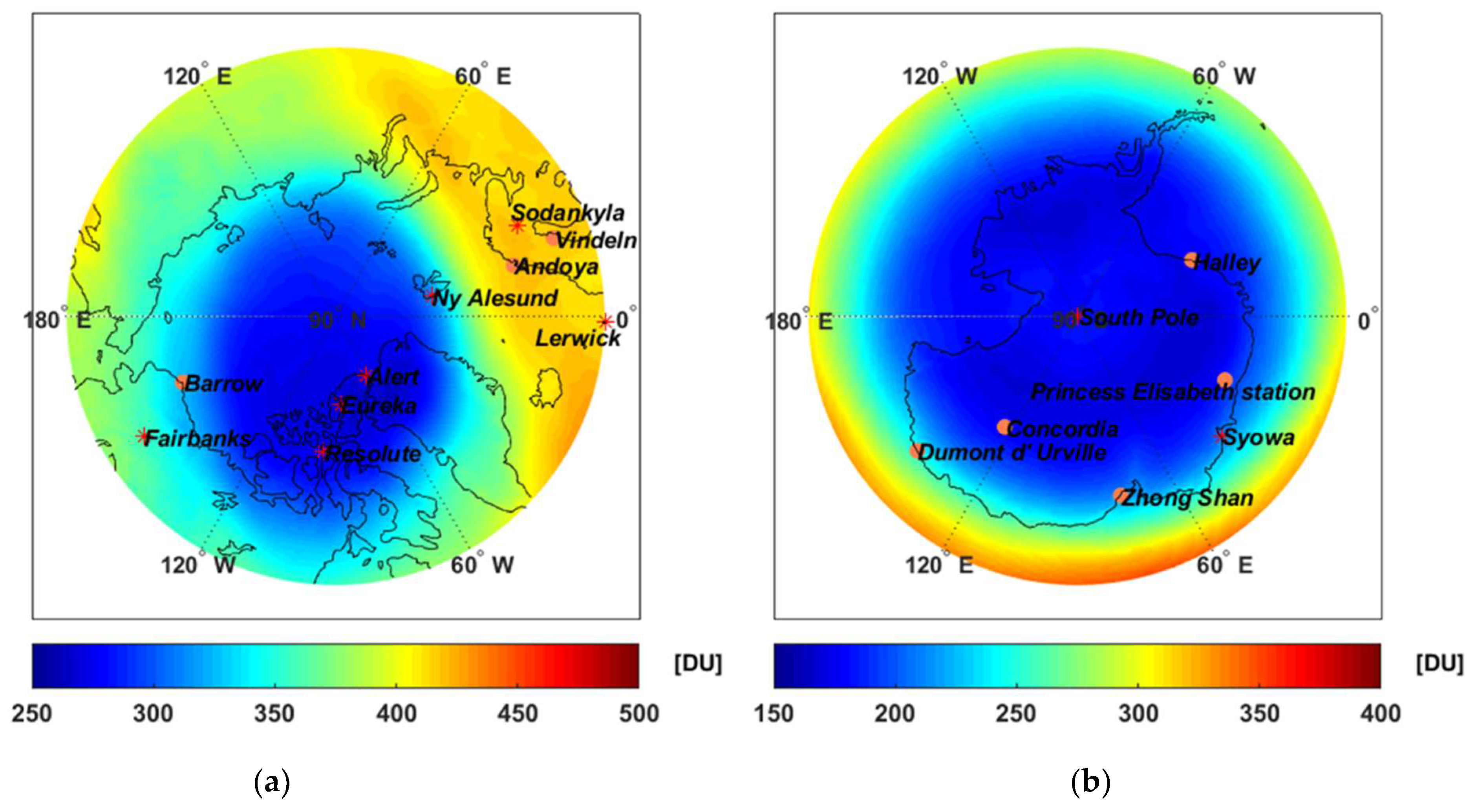
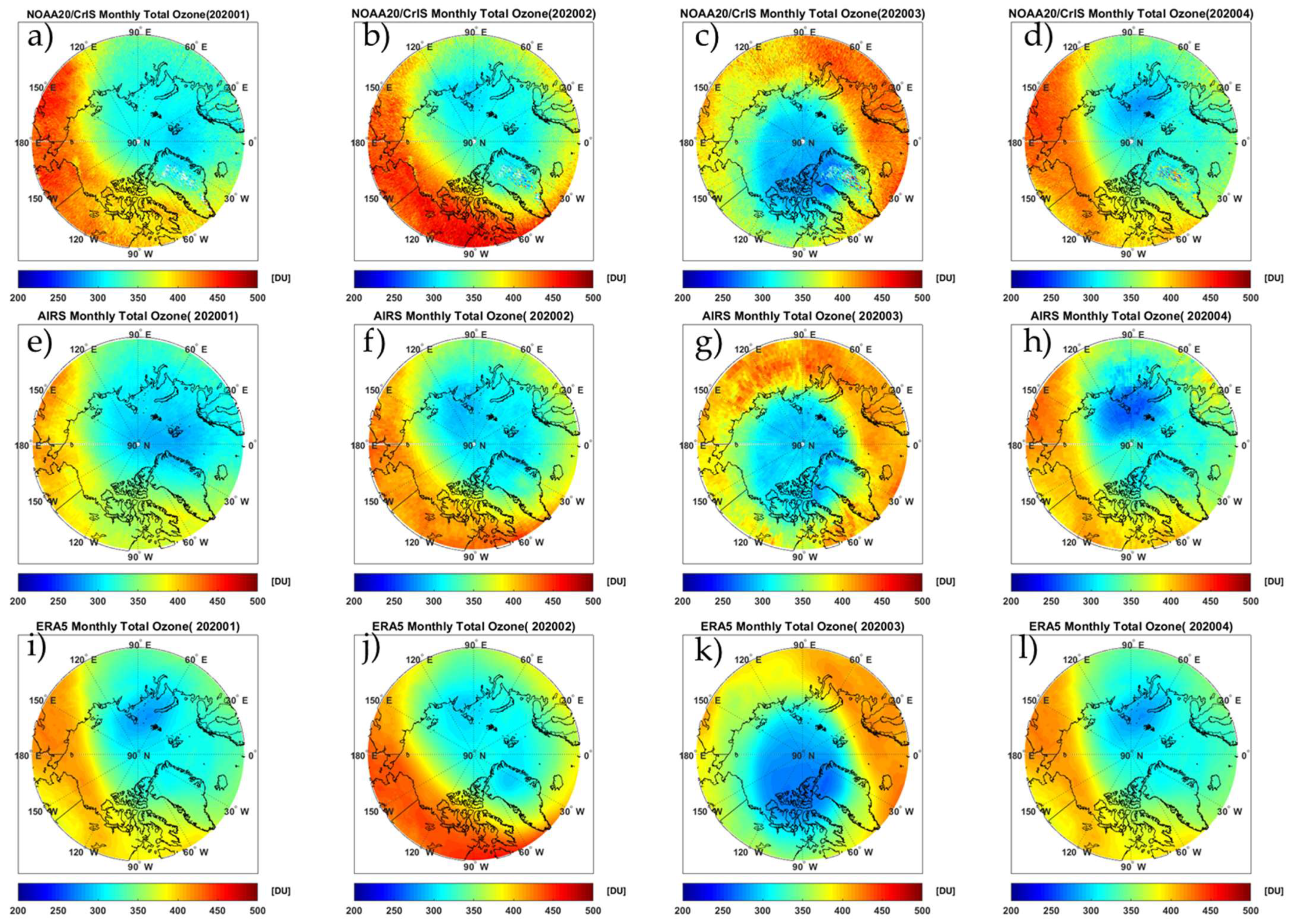
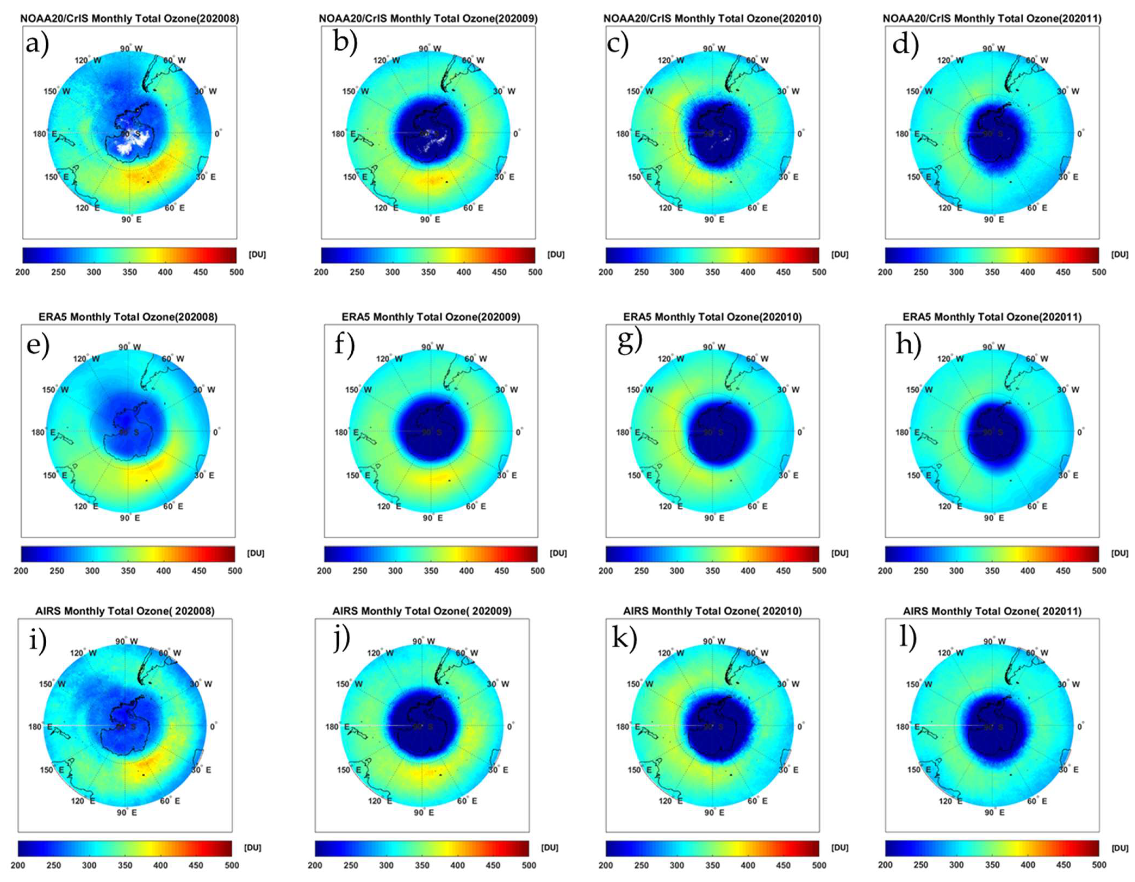
3.1. TCO Characteristics in Polar Regions

As shown in Figure 2, both satellite measurements of ozone (derived from AIRS and CrIS) and the ERA5 reanalysis ozone field could capture the spatial distribution of extreme ozone depletion in the Arctic in March 2020 (Figure 2c,g,k). However, the strength of ozone depletion indicated by the AIRS V7 ozone product (Figure 2g) was apparently weaker than that of CrIS (Figure 2c) and ERA5 (Figure 2k) in the central region of the Arctic in March 2020. In addition, it should be noted that although CrIS and AIRS both operate in polar orbit, with a high sample frequency and spatial coverage in polar regions, the available coverage passing the quality control selection criteria of AIRS and CrIS ozone products shows profound differences, which can be partly attributed to the inconsistency of the retrieval algorithm settings. The maximum difference can be seen in Greenland in the wintertime in the Arctic, especially on a daily scale. Similarly, it can be observed in winter in the southern hemisphere, such as on the Antarctic continent.
Figure 3 shows the development process of ozone loss in the Antarctic in 2020, which begins to decline around the end of August, reaches its minimum of approximately 120 Du by early October, and lasts until late November. The spatial consistency of the TCO among the three datasets (CrIS, AIRS, and ERA5) in the Antarctic region is significantly better than that in the Arctic, which reflects the fact that ozone retrieval based on AIRS and CrIS measurements is rather challenging in the Arctic due to the high variability of meteorological factors, e.g., temperature [58] and humidity profile [59]. The dependence of the rate of heterogeneous reactions on temperature and the influence of the accuracy of temperature and humidity profiles on ozone retrieval can be combined to explain the difference between the Arctic and Antarctic. Existing studies have shown that the interannual variability of temperature over the Arctic in winter and spring is higher than that over the Antarctic [58,60], which can increase the uncertainty of the AIRS and CrIS ozone retrieval algorithms and complicate further analysis and application.
In general, the differences in meteorological conditions and the limitations of the retrieval algorithm affect the TCO spatial distribution for CrIS and AIRS in the polar regions. In contrast, the ERA5 reanalysis data, due to the lack of observations for the assimilation process in the polar regions, mainly rely on the dynamic model and the parameterization scheme for the ozone field embedded within the model, and this is expected to obtain more consistent results in both polar regions.

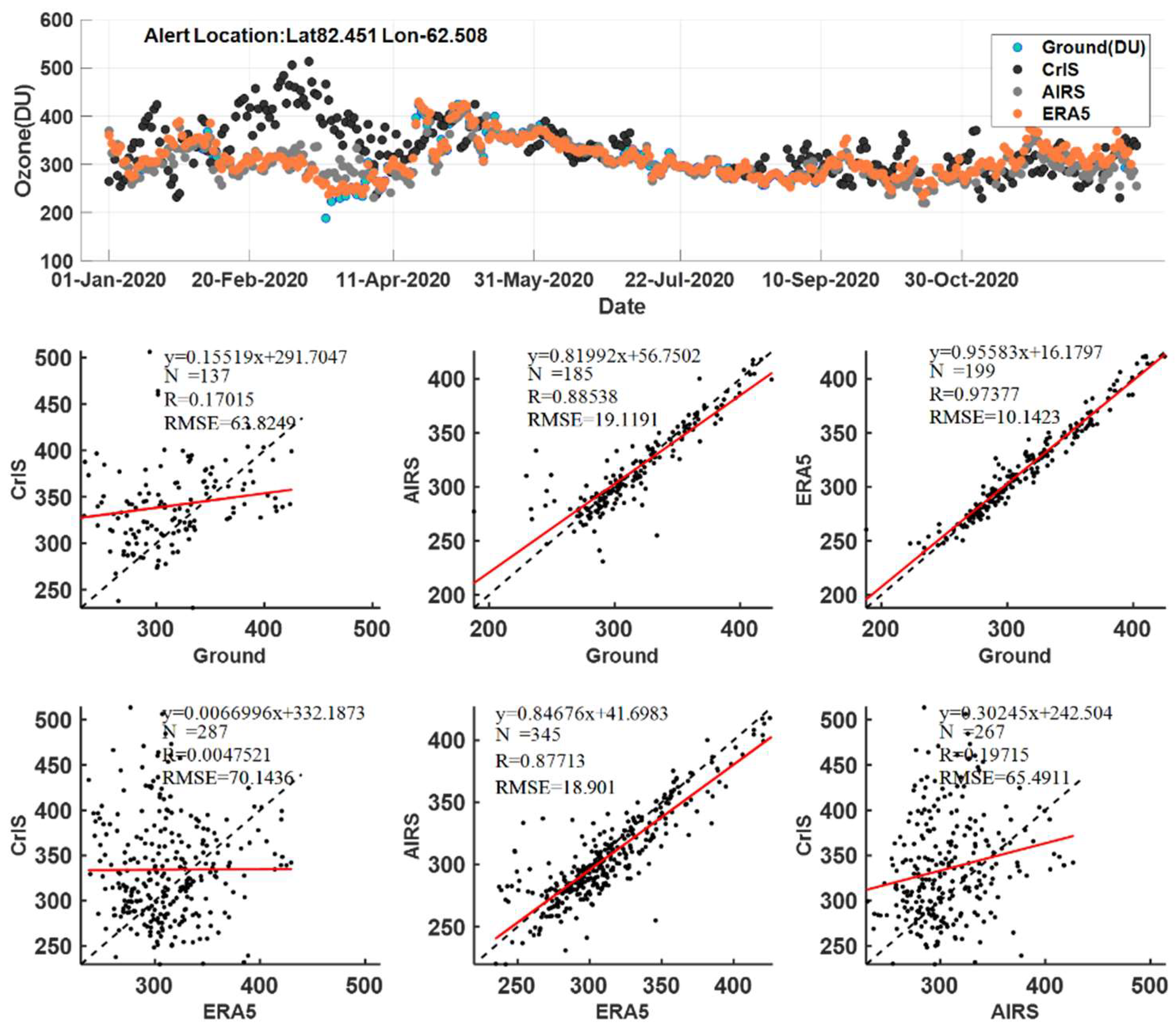
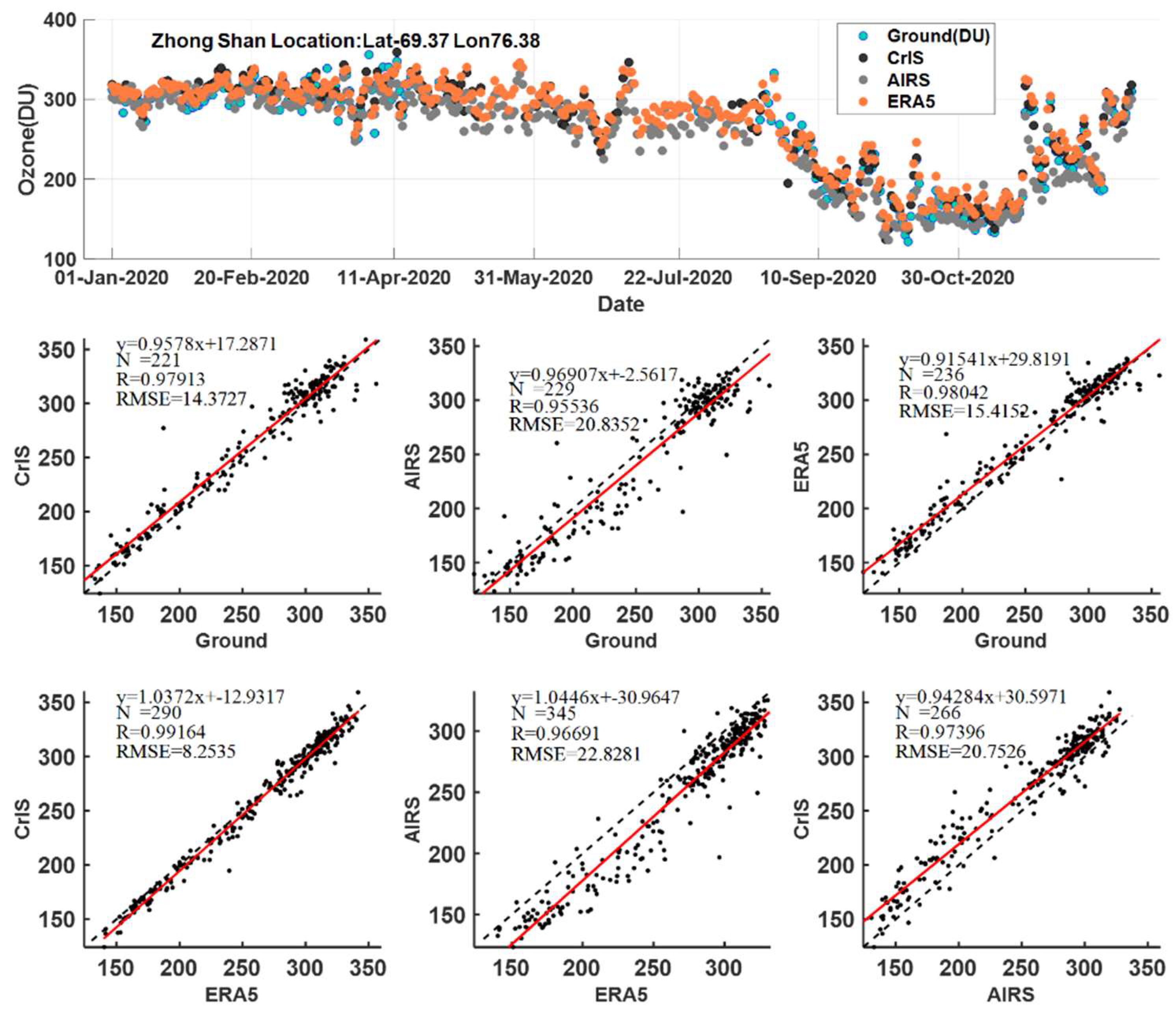
The Inter-Comparison of TCO

In order to evaluate the representativeness of the CrIS, AIRS, and ERA5 TCO datasets in the polar regions further, we selected three polar ground-based sites to represent different surface types and locations relative to the polar vortex; in addition, the number of matched pairs was also taken into consideration. Then, we conducted data screening and matching procedures according to the co-location criteria proposed in Section 2.4. The results are shown in Figure 4, Figure 5 and Figure 6. More information about other stations can be found in the Supplementary Materials.
Figure 4 shows the ground daily observations (blue) and CrIS (black), AIRS (grey), and ERA5 (orange) TCO sequences in 2020 at the Arctic Alert site. The Alert site is located on the coastline of Greenland and the Arctic Ocean. Although ground-based observations between 10 February and 10 March are missing, overall, the ozone products of AIRS and ERA5 show good agreement with ground-based observations. However, the CrIS TCO shows a large deviation and cannot reflect the ozone depletion at this site in spring 2020. A similar situation also occurs at the Eureka station (Latitude: 80.0500° N, longitude: −86.4167°), as can be seen in Figure S1. Boynard et al. [43] also pointed out that the IASI TCO shows the largest differences over the cold surface of Greenland compared with the GOME2 TCO during the March–April–May (MAM) season. As a control, the inter-comparison results at the Lerwick site are shown in Figure 5, located at 60.13° N and 1.18° W, which is far away from the central region of the Arctic ozone hole compared to the Alert site. At the Lerwick site, the consistency of the TCO between CrIS and ground-based observations is significantly improved from almost no correlation to a correlation of more than 0.93, accompanied by a consistency improvement between AIRS and ERA5. Figure S2 shows that the Vindeln station located at 64.24° N and 19.77° E also displays a consistency improvement compared with the Alert station, which is located at high latitude and is susceptible to polar vortices. Generally, ERA5 has the best spatial consistency with each ground site (over 0.96) and is not affected by the location of the site. Moreover, AIRS can also capture the spatial–temporal characteristics of TCO variation at each site even under extreme conditions.
Figure 6 further analyzes the performance of the four types of TCO datasets at the Zhongshan station in Antarctica. Ground-based observations from April 2020 to August 2020 are missing, but all four datasets capture the ozone hole variation in winter/spring 2020 in the Antarctic, and they show good consistency with each other, during both the ozone hole and non-ozone hole period. The total amount of ozone at this site varies from 120 DU to 350 DU, and CrIS shows the best consistency with the ground-based TCO, with the smallest RMSE and highest correlation, followed by the ERA5 TCO. In contrast, the AIRS TCO results at the Zhongshan site are systematically lower than those of the ground-based observations; they also have a large RMSE, and the underestimation is more obvious between ERA5 and AIRS. The TCO comparison results between ERA5 and ground-based values indicate that ERA5 exhibits an overestimation, especially during the ozone hole period. The South Pole station (Latitude: −89.9969° N, longitude: −24.8000°) also shows good consistency among the ERA5 and ground-based observations (as seen in Figure S3), but the available observations derived from CrIS and AIRS were too few to calculate statistical metrics. Detailed statistical metrics can be found in Table 2.

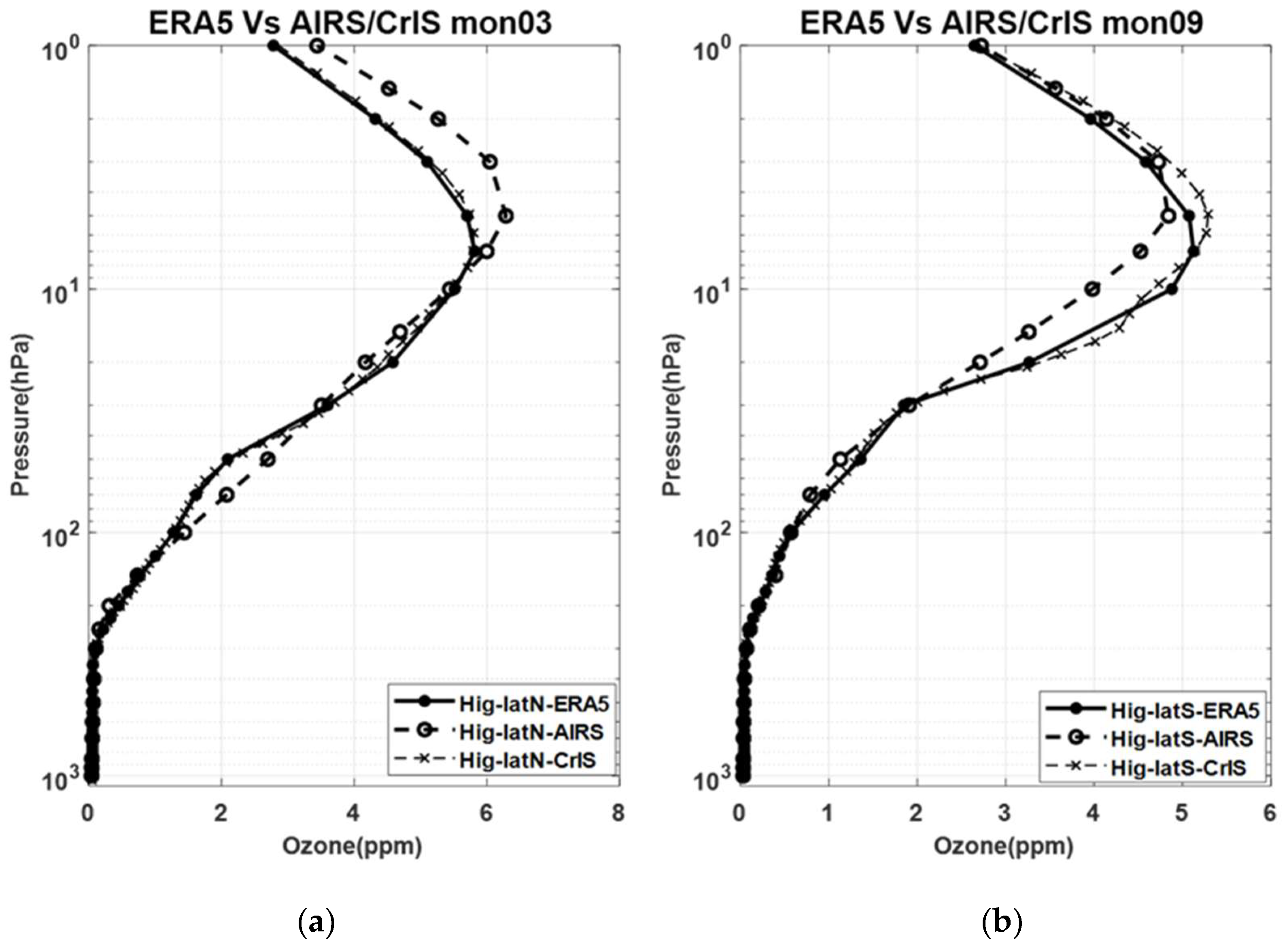
3.2. Ozone Profile Characteristics during the Polar Ozone Hole

Figure 7 shows the vertical distribution characteristics of the CrIS (solid circle, solid line), AIRS (open circles, dashed line), and ERA5 (cross dashed line) ozone profiles in the high-latitude zones of the northern hemisphere (NH) and southern hemisphere (SH) during the ozone hole period in March and September 2020, respectively, on the monthly scale. The high-latitude zones defined here are those with a latitude range within 60°~90° N or 60°~90° S. Qualitatively, it can be seen from Figure 7a that the ozone profile provided by CrIS is highly consistent with that of ERA5 for March 2020 in the Arctic, but it has an obvious difference from the vertical distribution of AIRS above 10 hPa. At altitudes of 10 hPa to 1 hPa, the AIRS ozone values are significantly higher than those of CrIS and ERA5, which can account for the TCO overestimation of AIRS compared to CrIS and ERA5 in the middle row of Figure 2, due to the significant contribution to the total amount of ozone in this altitude range. Furthermore, the obvious difference in the vertical distribution shapes of the profile on the monthly mean scale may be related to the difference in the ozone prior profiles in the CrIS and AIRS physical retrievals. The ozone prior profiles of CrIS are derived from the MERRA2 reanalysis datasets, so the consistency between MERRA2 and the ERA5 ozone field for high-latitudes zones on the monthly scale may explain the high consistency of the ozone profile between CrIS and ERA5 in this area. Meanwhile, AIRS ozone physical retrieval uses the ozone profile generated by the SCCNN process a priori. Figure 7b is the same as Figure 7a, but for the SH in September 2020. Compared with the Arctic in March, the minimum and maximum ozone values during the Antarctic ozone hole period are substantially lower. Similarly, the vertical distribution of the CrIS ozone profile is still highly consistent with that of ERA5 in September 2020 in the Antarctic; however, the ozone profile of AIRS is significantly lower than that of ERA5 and CrIS between 50 hPa and 10 hPa. It should be noted that the monthly mean ozone profiles displayed in Figure 7 all refer to their own pressure layers without interpolation.

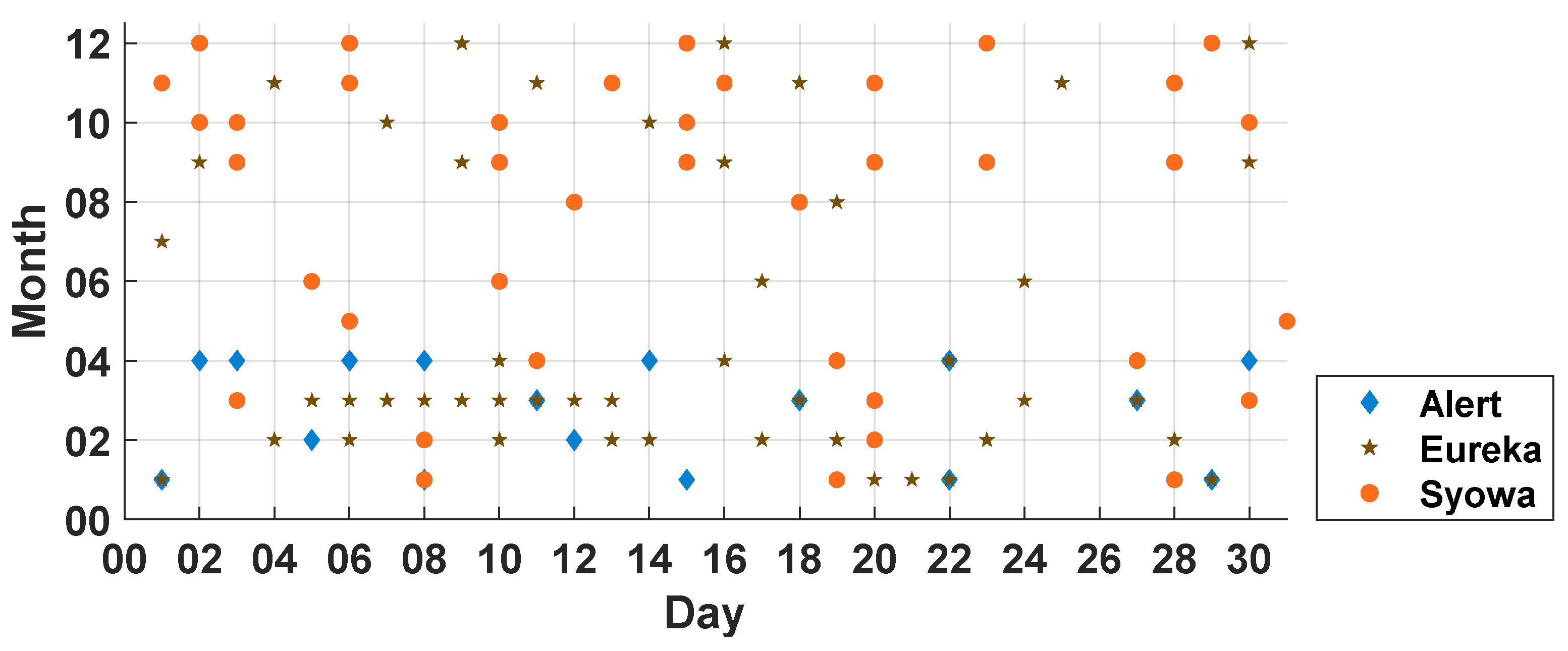
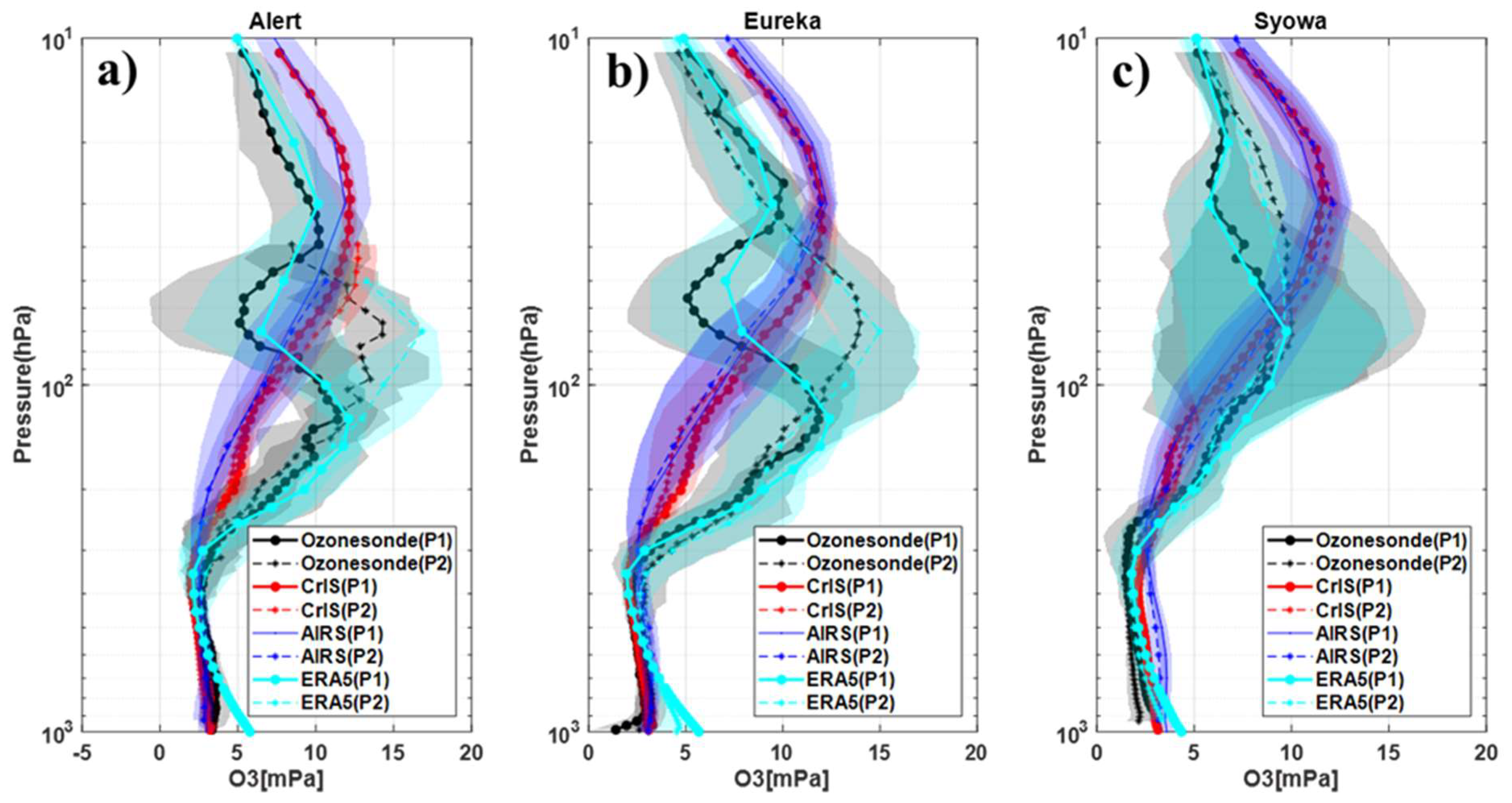
Comparison with Ozonesonde

In order to evaluate the performance of the CrIS, AIRS, and ERA5 ozone profile datasets in the polar regions, especially during the ozone loss season, the ozonesonde observations obtained from three in situ sites (Alert and Eureka stations in NH and Syowa station in SH) were used as references. The observation sequences were divided into two phases to separate the ozone hole (P1) and non-ozone hole period (P2). The division of each site and the number of observations within each phase are shown in Table 3. Figure 8 depicts the temporal distribution of ozonesonde observations in 2020, in which each dot shape indicates the observation month (y-axis) and day (x-axis).
Figure 9 shows the inter-comparison of the ozone profiles of CrIS, AIRS, ERA5, and ozonesonde during the P1 and P2 phases, respectively. The black solid line represents the average value of ozonesonde observations during the P1 stage, and the dotted line represents the average value of the ozonesonde observations during the P2 stage. Analogously, red, blue, and turquoise along with solid lines and dashed lines represent the average values of CrIS, AIRS, and ERA5 in the P1 and P2 stages, respectively, with the shading representing the standard deviation of each item. The differences between the dotted lines and the solid lines quantitatively indicate the depth and location of ozone depletion at the three sites displayed by the four types of ozone profile datasets. Generally, the ozonesonde results indicate that the maximum ozone value is below 5 ppm. At the Alert and Eureka sites, ozone depletion mainly occurs at the altitude range of 100 hPa to 50 hPa, and the difference between the P1 and P2 stages can reach 2 ppm. At higher altitudes above 50 hPa, ozone values displayed in the P2 phase are greater than those in the P1 phase. Meanwhile, the ozone depletion at Syowa, which represents Antarctica, mainly occurs above 50 hPa. It should be noted that no statistical conclusions can be drawn because the results are limited to the site location and the years in which the observations were conducted, since the location and strength of ozone depletion have obvious spatiotemporal and interannual variations. Correspondingly, the ERA5 ozone profiles can accurately capture the characteristics of ozone changes in polar regions in terms of not only magnitude but also shape. In contrast, the CrIS and AIRS ozone profiles perform poorly in the polar regions. Moreover, the shapes of the CrIS ozone profiles in the polar regions cannot clearly distinguish between the P1 and P2 stages and also cannot reflect the depth or location of ozone depletion. AIRS is slightly better than CrIS in distinguishing the P1 and P2 stages; for example, the difference between the blue solid line and the dashed line can be seen for the Syowa site in Antarctica. This slight difference in the detection capability may be associated with the improvement related to ozone retrieval and the quality control strategy implemented in the recently released AIRS version 7 ozone products, e.g., a prior profile suitable for the ozone hole period is selected according to the temperature values at the height of 50 hPa derived from the SCCNN procedure.

4. Conclusions

This paper evaluated three ozone datasets (CrIS/NOAA 20, AIRS/Aqua, ERA5/ECWMF) in the high latitudes of the northern and southern hemispheres in 2020. The performance and applicability of the ozone profiles obtained from CrIS, AIRS, and the ERA5 reanalysis data were evaluated in the polar regions. The results showed that the ERA5 reanalysis ozone field is superior to the CrIS/NOAA20 and AIRS v7 ozone products, not only in terms of temporal and spatial coverage but also in terms of consistency with ground-based observations. Thus, ERA5 reanalysis ozone data are more applicable in studies of the polar ozone. The limitations of CrIS and AIRS ozone data during the polar ozone hole period can be summarized as follows:
(1)
Insufficient spatial coverage. Firstly, due to some factors—for example, the influence of clouds—the AIRS and CrIS ozone products are unable to cover areas with thick cloud. The difference in algorithm settings regarding quality control also affects the data usage, which leads to a difference in spatial coverage between CrIS and AIRS. In addition, we also found that the number of available observations of CrIS was lower than that of AIRS over the continental area in the polar wintertime and springtime, such as the Antarctic continent in August 2020 and Greenland in January 2020.
(2)
Inability to represent ozone profile vertical structure effectively in polar regions. It is difficult for both CrIS and AIRS ozone profiles to capture the strength and location of ozone loss in the vertical direction compared with ozonesonde and ERA5, regardless of whether this is during the ozone or non-ozone loss period. This is related to the low detection sensitivity of thermal infrared techniques. On the other hand, the strong dependence of the ozone retrieval algorithm on a prior profile acquired under low-temperature environmental conditions could also account for this limitation. In addition, other different factors that make measurements of the ozone profile rather challenging in the polar regions, such as the complex and mixed ice, snow, and water surface conditions, especially the sea ice, increase the complexity of the surface parameters that can be characterized by retrieval algorithms.
The TCO comparison between the South Pole and North Pole demonstrated that the performance of CrIS at the Alert site was significantly inferior to its performance at sites in the Antarctic or outside the Arctic polar vortex, especially during the period of the ozone hole. The location of the alert site can partly account for this result, as well as high variability of climate variables in the Arctic [58,59,61]. In addition, it should be noted that the ERA5 reanalysis ozone data in comparison with CrIS/NOAA20 and AIRS/Aqua data over both polar regions for the winter- and spring-time of 2020 integrate a wide range of TCO satellite measurement datasets. Furthermore, the Arctic ozone hole needs to be studied, including its atmospheric variation and surface properties, in order to improve our understanding of this event, which will also help in performing targeted algorithm improvements during the Arctic ozone hole.

Supplementary Materials

The following are available online at https://www.mdpi.com/article/10.3390/rs13214375/s1, Figure S1: The time series of total column ozone (CrIS/AIRS/ERA5 and ground-based instruments) at Eureka site, Figure S2: The comparison of total column ozone between matched CrIS/AIRS/ERA5 and ground-based instruments at VindeIn site. Upper row: the time series of total column ozone; Middle and bottom rows: inter-comparison scatter plots with each other, Figure S3: The time series of total column ozone (CrIS/AIRS/ERA5 and ground-based instruments) at South Pole site.

Author Contributions

Conceptualization, Y.W. and L.C.; Data curation, K.C.; Formal analysis, Y.W. and S.Z.; Methodology, H.W. and Y.W.; Project administration, H.W.; Resources, H.W.; Validation, H.W. and X.Z.; Writing—original draft, H.W. All authors have read and agreed to the published version of the manuscript.

Funding

This research is supported by the Open Fund of the State Key Laboratory of Remote Sensing Science (Grant Number OFSLRSS201913) and the National Natural Science Foundation of China (Grant Number 41901269).

Institutional Review Board Statement

Not applicable.

Informed Consent Statement

Not applicable.

Data Availability Statement

Not applicable.

Acknowledgments

We wish to thank the AIRS Science Team and the CrIS Science Team who prepared and provided the AIRS V7 and CLIMCAPS ozone datasets used in this study. The authors are grateful to WOUDC for the open access to ground-based ozone measurements. We are sincerely grateful to ECWMF for the free release of the ERA5 reanalysis data. We also thank Lei Zhang for his strong support of the data process method discussion.

Conflicts of Interest

The authors declare no conflict of interest.

References

  1. Son, S.-W.; Polvani, L.M.; Waugh, D.W.; Akiyoshi, H.; Garcia, R.; Kinnison, D.; Pawson, S.; Rozanov, E.; Shepherd, T.G.; Shibata, K. The impact of stratospheric ozone recovery on the southern hemisphere westerly jet. Science 2008, 320, 1486–1489. [Google Scholar] [CrossRef]
  2. Shindell, D.; Rind, D.; Balachandran, N.; Lean, J.; Lonergan, P. Solar cycle variability, ozone, and climate. Science 1999, 284, 305–308. [Google Scholar] [CrossRef] [Green Version]
  3. Xie, F.; Tian, W.; Chipperfield, M.P. Radiative effect of ozone change on stratosphere-troposphere exchange. J. Geophys. Res. Atmos. 2008, 113, 113. [Google Scholar] [CrossRef] [Green Version]
  4. Zhang, J.; Tian, W.; Xie, F.; Pyle, J.A.; Keeble, J.; Wang, T. The influence of zonally asymmetric stratospheric ozone changes on the arctic polar vortex shift. J. Clim. 2020, 33, 4641–4658. [Google Scholar] [CrossRef] [Green Version]
  5. Sillman, S. The relation between ozone, NOx and hydrocarbons in urban and polluted rural environments. Atmos. Environ. 1999, 33, 1821–1845. [Google Scholar] [CrossRef]
  6. Monks, P.S.; Archibald, A.T.; Colette, A.; Cooper, O.; Coyle, M.; Derwent, R.; Fowler, D.; Granier, C.; Law, K.S.; Mills, G.E.; et al. Tropospheric ozone and its precursors from the urban to the global scale from air quality to short-lived climate forcer. Atmos. Chem. Phys. 2015, 15, 8889–8973. [Google Scholar] [CrossRef] [Green Version]
  7. Deshler, T.; Mercer, J.L.; Smit, H.G.J.; Stubi, R.; Levrat, G.; Johnson, B.J.; Oltmans, S.J.; Kivi, R.; Thompson, A.M.; Witte, J.; et al. Atmospheric comparison of electrochemical cell ozonesondes from different manufacturers, and with different cathode solution strengths: The balloon experiment on standards for ozonesondes. J. Geophys. Res. Atmos. 2008, 113. [Google Scholar] [CrossRef]
  8. Tarasick, D.W.; Smit, H.G.J.; Thompson, A.M.; Morris, G.A.; Witte, J.C.; Davies, J.; Nakano, T.; Van Malderen, R.; Stauffer, R.M.; Johnson, B.J.; et al. Improving ECC ozonesonde data quality: Assessment of current methods and outstanding issues. Earth Space Sci. 2021, 8. [Google Scholar] [CrossRef]
  9. Komhyr, W.D.; Grass, R.D.; Leonard, R.K. Dobson spectrophotometer 83: A standard for total ozone measurements, 1962–1987. J. Geophys. Res. Atmos. 1989, 94, 9847–9861. [Google Scholar] [CrossRef]
  10. Balis, D.; Kroon, M.; Koukouli, M.E.; Brinksma, E.J.; Labow, G.; Veefkind, J.P.; McPeters, R.D. Validation of Ozone Monitoring Instrument total ozone column measurements using Brewer and Dobson spectrophotometer ground-based observations. J. Geophys. Res. Atmos. 2007, 112. [Google Scholar] [CrossRef] [Green Version]
  11. Kerr, J.B.; Asbridge, I.A.; Evans, W.F.J. Intercomparison of total ozone measured by the Brewer and Dobson spectrophotometers at Toronto. J. Geophys. Res. Atmos. 1988, 93, 11129–11140. [Google Scholar] [CrossRef]
  12. Sullivan, J.T.; McGee, T.J.; Sumnicht, G.K.; Twigg, L.W.; Hoff, R.M. A mobile differential absorption lidar to measure sub-hourly fluctuation of tropospheric ozone profiles in the Baltimore-Washington, DC region. Atmos. Meas. Tech. 2014, 7, 3529–3548. [Google Scholar] [CrossRef] [Green Version]
  13. Wang, L.; Newchurch, M.J.; Alvarez, R.J., II; Berkoff, T.A.; Brown, S.S.; Carrion, W.; De Young, R.J.; Johnson, B.J.; Ganoe, R.; Gronoff, G.; et al. Quantifying TOLNet ozone lidar accuracy during the 2014 DISCOVER-AQ and FRAPPE campaigns. Atmos. Meas. Tech. 2017, 10, 3865–3876. [Google Scholar] [CrossRef] [PubMed] [Green Version]
  14. Gelaro, R.; McCarty, W.; Suárez, M.J.; Todling, R.; Molod, A.; Takacs, L.; Randles, C.A.; Darmenov, A.; Bosilovich, M.G.; Reichle, R.; et al. The modern-era retrospective analysis for research and applications, version 2 (MERRA-2). J. Clim. 2017, 30, 5419–5454. [Google Scholar] [CrossRef]
  15. Inness, A.; Ades, M.; Agusti-Panareda, A.; Barre, J.; Benedictow, A.; Blechschmidt, A.-M.; Dominguez, J.J.; Engelen, R.; Eskes, H.; Flemming, J.; et al. The CAMS reanalysis of atmospheric composition. Atmos. Chem. Phys. 2019, 19, 3515–3556. [Google Scholar] [CrossRef] [Green Version]
  16. Hersbach, H.; Bell, B.; Berrisford, P.; Hirahara, S.; Horanyi, A.; Munoz-Sabater, J.; Nicolas, J.; Peubey, C.; Radu, R.; Schepers, D.; et al. The ERA5 global reanalysis. Q. J. R. Meteorol. Soc. 2020, 146, 1999–2049. [Google Scholar] [CrossRef]
  17. Fujiwara, M.; Wright, J.S.; Manney, G.L.; Gray, L.J.; Anstey, J.; Birner, T.; Davis, S.; Gerber, E.P.; Harvey, V.L.; Hegglin, M.I.; et al. Introduction to the SPARC Reanalysis Intercomparison Project (S-RIP) and overview of the reanalysis systems. Atmos. Chem. Phys. 2017, 17, 1417–1452. [Google Scholar] [CrossRef] [Green Version]
  18. Molod, A.; Takacs, L.; Suarez, M.; Bacmeister, J. Development of the GEOS-5 atmospheric general circulation model: Evolution from MERRA to MERRA2. Geosci. Model Dev. 2015, 8, 1339–1356. [Google Scholar] [CrossRef] [Green Version]
  19. Kobayashi, S.; Ota, Y.; Harada, Y.; Ebita, A.; Moriya, M.; Onoda, H.; Onogi, K.; Kamahori, H.; Kobayashi, C.; Endo, H.; et al. The JRA-55 reanalysis: General specifications and basic characteristics. J. Meteorol. Soc. Jpn. Ser. II 2015, 93, 5–48. [Google Scholar] [CrossRef] [Green Version]
  20. Wargan, K.; Labow, G.; Frith, S.; Pawson, S.; Livesey, N.; Partyka, G. Evaluation of the ozone fields in NASA’s MERRA-2 reanalysis. J. Clim. 2017, 30, 2961–2988. [Google Scholar] [CrossRef] [Green Version]
  21. Dethof, A.; Holm, E.V. Ozone assimilation in the ERA-40 reanalysis project. Q. J. R. Meteorol. Soc. 2004, 130, 2851–2872. [Google Scholar] [CrossRef]
  22. Dragani, R. On the quality of the ERA-Interim ozone reanalyses: Comparisons with satellite data. Q. J. R. Meteorol. Soc. 2011, 137, 1312–1326. [Google Scholar] [CrossRef]
  23. Ziemke, J.R.; Olsen, M.A.; Witte, J.C.; Douglass, A.R.; Strahan, S.E.; Wargan, K.; Liu, X.; Schoeberl, M.R.; Yang, K.; Kaplan, T.B.; et al. Assessment and applications of NASA ozone data products derived from Aura OMI/MLS satellite measurements in context of the GMI chemical transport model. J. Geophys. Res. Atmos. 2014, 119, 5671–5699. [Google Scholar] [CrossRef]
  24. Orr, A.; Lu, H.; Martineau, P.; Gerber, E.P.; Marshall, G.J.; Bracegirdle, T.J. Is our dynamical understanding of the circulation changes associated with the Antarctic ozone hole sensitive to the choice of reanalysis dataset? Atmos. Chem. Phys. 2021, 21, 7451–7472. [Google Scholar] [CrossRef]
  25. Inness, A.; Chabrillat, S.; Flemming, J.; Huijnen, V.; Langenrock, B.; Nicolas, J.; Polichtchouk, I.; Razinger, M. Exceptionally low arctic stratospheric ozone in spring 2020 as seen in the CAMS reanalysis. J. Geophys. Res. Atmos. 2020, 125, 125. [Google Scholar] [CrossRef]
  26. Solomon, S.; Garcia, R.R.; Rowland, F.S.; Wuebbles, D.J. On the depletion of Antarctic ozone. Nature 1986, 321, 755–758. [Google Scholar] [CrossRef] [Green Version]
  27. Langematz, U.; Tully, M.; Calvo, N.; Dameris, M.; Young, P. Polar Stratospheric Ozone: Past, Present, and Future Chapter 4 in WMO Scientific Assessment of Ozone Depletion: 2018; German Aerospace Center: Cologne, Germany, 2018. [Google Scholar]
  28. Chipperfield, M.P.; Bekki, S.; Dhomse, S.; Harris, N.R.P.; Hassler, B.; Hossaini, R.; Steinbrecht, W.; Thieblemont, R.; Weber, M. Detecting recovery of the stratospheric ozone layer. Nature 2017, 549, 211–218. [Google Scholar] [CrossRef] [PubMed] [Green Version]
  29. Solomon, S.; Haskins, J.; Ivy, D.J.; Min, F. Fundamental differences between Arctic and Antarctic ozone depletion. Proc. Natl. Acad. Sci. USA 2014, 111, 6220–6225. [Google Scholar] [CrossRef] [Green Version]
  30. Solomon, S.; Kinnison, D.; Bandoro, J.; Garcia, R. Simulation of polar ozone depletion: An update. J. Geophys. Res. Atmos. 2015, 120, 7958–7974. [Google Scholar] [CrossRef]
  31. Manney, G.L.; Santee, M.L.; Rex, M.; Livesey, N.J.; Pitts, M.C.; Veefkind, P.; Nash, E.R.; Wohltmann, I.; Lehmann, R.; Froidevaux, L.; et al. Unprecedented Arctic ozone loss in 2011. Nature 2011, 478, 469–475. [Google Scholar] [CrossRef] [PubMed]
  32. Feng, W.; Dhomse, S.S.; Arosio, C.; Weber, M.; Burrows, J.P.; Santee, M.L.; Chipperfield, M.P. Arctic ozone depletion in 2019/20: Roles of chemistry, dynamics and the Montreal Protocol. Geophys. Res. Lett. 2021, 48. [Google Scholar] [CrossRef]
  33. Lawrence, Z.D.; Perlwitz, J.; Butler, A.H.; Manney, G.L.; Newman, P.A.; Lee, S.H.; Nash, E.R. The remarkably strong Arctic stratospheric polar vortex of winter 2020: Links to record-breaking Arctic oscillation and ozone loss. J. Geophys. Res. Atmos. 2020, 125. [Google Scholar] [CrossRef]
  34. Stolarski, R.S.; McPeters, R.D.; Newman, P.A. The ozone hole of 2002 as measured by TOMS. J. Atmos. Sci. 2005, 62, 716–720. [Google Scholar] [CrossRef]
  35. Weber, M.; Arosio, C.; Feng, W.; Dhomse, S.S.; Chipperfield, M.P.; Meier, A.; Burrows, J.P.; Eichmann, K.-U.; Richter, A.; Rozanov, A. The unusual stratospheric arctic winter 2019/20: Chemical ozone loss from satellite observations and TOMCAT chemical transport model. J. Geophys. Res. Atmos. 2021, 126. [Google Scholar] [CrossRef]
  36. Dameris, M.; Loyola, D.G.; Nutzel, M.; Coldewey-Egbers, M.; Lerot, C.; Romahn, F.; van Roozendael, M. Record low ozone values over the Arctic in boreal spring 2020. Atmos. Chem. Phys. 2021, 21, 617–633. [Google Scholar] [CrossRef]
  37. Rao, J.; Garfinkel, C.I. Arctic ozone loss in March 2020 and its seasonal prediction in CFSv2: A comparative study with the 1997 and 2011 cases. J. Geophys. Res. Atmos. 2020, 125, 125. [Google Scholar] [CrossRef]
  38. DeLand, M.T.; Bhartia, P.K.; Kramarova, N.; Chen, Z. OMPS LP Observations of PSC variability during the NH 2019-2020 season. Geophys. Res. Lett. 2020, 47, 47. [Google Scholar] [CrossRef]
  39. Manney, G.L.; Livesey, N.J.; Santee, M.L.; Froidevaux, L.; Lambert, A.; Lawrence, Z.D.; Millan, L.F.; Neu, J.L.; Read, W.G.; Schwartz, M.J.; et al. Record-low Arctic stratospheric ozone in 2020: MLS Observations of chemical processes and comparisons with previous extreme winters. Geophys. Res. Lett. 2020, 47. [Google Scholar] [CrossRef]
  40. Hu, Y. The very unusual polar stratosphere in 2019–2020. Sci. Bull. 2020, 65, 1775–1777. [Google Scholar] [CrossRef]
  41. Zhang, L.; Ding, M.; Bian, L.; Li, J. Validation of AIRS temperature and ozone profiles over Antarctica. Chin. J. Geophys. Chin. Ed. 2020, 63, 1318–1331. [Google Scholar] [CrossRef]
  42. Smith, N.; Barnet, C.D. CLIMCAPS observing capability for temperature, moisture, and trace gases from AIRS/AMSU and CrIS/ATMS. Atmos. Meas. Tech. 2020, 13, 4437–4459. [Google Scholar] [CrossRef]
  43. Boynard, A.; Hurtmans, D.; Garane, K.; Goutail, F.; Hadji-Lazaro, J.; Koukouli, M.E.; Wespes, C.; Vigouroux, C.; Keppens, A.; Pommereau, J.-P.; et al. Validation of the IASI FORLI/EUMETSAT ozone products using satellite (GOME-2), ground-based (Brewer-Dobson, SAOZ, FTIR) and ozonesonde measurements. Atmos. Meas. Tech. 2018, 11, 5125–5152. [Google Scholar] [CrossRef] [Green Version]
  44. Yue, Q.; Lambrigtsen, B. AIRS Version 7 Level 2 Performance Test and Validation Report; Jet Propulsion Laboratory, California Institute of Technology: Pasadena, CA, USA, 2020. [Google Scholar]
  45. Thrastarson, H.T.; Olsen, E.T. AIRS/AMSU/HSB Version 7 Level 2 Quality Control and Error Estimation; Jet Propulsion Laboratory, California Institute of Technology: Pasadena, CA, USA, 2020. [Google Scholar]
  46. Kim, J.; Kim, J.; Cho, H.K.; Herman, J.; Park, S.S.; Lim, H.K.; Kim, J.H.; Miyagawa, K.; Lee, Y.G. Intercomparison of total column ozone data from the Pandora spectrophotometer with Dobson, Brewer, and OMI measurements over Seoul, Korea. Atmos. Meas. Tech. 2017, 10, 3661–3676. [Google Scholar] [CrossRef] [Green Version]
  47. Garane, K.; Koukouli, M.-E.; Verhoelst, T.; Lerot, C.; Heue, K.-P.; Fioletov, V.; Balis, D.; Bais, A.; Bazureau, A.; Dehn, A.; et al. TROPOMI/S5P total ozone column data: Global ground-based validation and consistency with other satellite missions. Atmos. Meas. Tech. 2019, 12, 5263–5287. [Google Scholar] [CrossRef] [Green Version]
  48. Nalli, N.R.; Gambacorta, A.; Liu, Q.; Tan, C.; Iturbide-Sanchez, F.; Barnet, C.D.; Joseph, E.; Morris, V.R.; Oyola, M.; Smith, J.W. Validation of atmospheric profile retrievals from the SNPP NOAA-unique combined atmospheric processing system. Part 2: Ozone. IEEE Trans. Geosci. Remote Sens. 2018, 56, 598–607. [Google Scholar] [CrossRef]
  49. Nassar, R.; Logan, J.A.; Worden, H.M.; Megretskaia, I.A.; Bowman, K.W.; Osterman, G.B.; Thompson, A.M.; Tarasick, D.W.; Austin, S.; Claude, H.; et al. Validation of Tropospheric Emission Spectrometer (TES) nadir ozone profiles using ozonesonde measurements. J. Geophys. Res. Atmos. 2008, 113. [Google Scholar] [CrossRef] [Green Version]
  50. Smith, N.; Barnet, C.D. Uncertainty Characterization and Propagation in the Community Long-Term Infrared Microwave Combined Atmospheric Product System (CLIMCAPS). Remote Sens. 2019, 11, 1227. [Google Scholar] [CrossRef] [Green Version]
  51. Gambacorta, A.; Barnet, C.D. Methodology and information content of the NOAA NESDIS operational channel selection for the Cross-Track Infrared Sounder (CrIS). IEEE Trans. Geosci. Remote Sens. 2013, 51, 3207–3216. [Google Scholar] [CrossRef]
  52. Susskind, J.; Blaisdell, J.M.; Iredell, L.; Keita, F. Improved Temperature sounding and quality control methodology using AIRS/AMSU Data: The AIRS Science Team version 5 retrieval algorithm. IEE Trans. Geosci. Remote Sens. 2011, 49, 883–907. [Google Scholar] [CrossRef] [Green Version]
  53. Aumann, H.H.; Chahine, M.T.; Gautier, C.; Goldberg, M.D.; Kalnay, E.; McMillin, L.M.; Revercomb, H.; Rosenkranz, P.W.; Smith, W.L.; Staelin, D.H.; et al. AIRS/AMSU/HSB on the aqua mission: Design, science objectives, data products, and processing systems. IEEE Trans. Geosci. Remote Sens. 2003, 41, 253–264. [Google Scholar] [CrossRef] [Green Version]
  54. Milstein, A.B.; Blackwell, W.J. Neural network temperature and moisture retrieval algorithm validation for AIRS/AMSU and CrIS/ATMS. J. Geophys. Res. Atmos. 2016, 121, 1414–1430. [Google Scholar] [CrossRef] [Green Version]
  55. Thrastarson, H.T.; Olsen, E.T. AIRS Version 7 Retrieval Channel Sets; Jet Propulsion Laboratory, California Institute of Technology: Pasadena, CA, USA, 2020. [Google Scholar]
  56. Susskind, J.; Blaisdell, J.M.; Iredell, L. Improved methodology for surface and atmospheric soundings, error estimates, and quality control procedures: The atmospheric infrared sounder science team version-6 retrieval algorithm. J. Appl. Remote Sens. 2014, 8. [Google Scholar] [CrossRef]
  57. Cariolle, D.; Teyssedre, H. A revised linear ozone photochemistry parameterization for use in transport and general circulation models: Multi-annual simulations. Atmos. Chem. Phys. 2007, 7, 2183–2196. [Google Scholar] [CrossRef] [Green Version]
  58. Chylek, P.; Folland, C.K.; Lesins, G.; Dubey, M.K.; Wang, M. Arctic air temperature change amplification and the Atlantic Multidecadal Oscillation. Geophys. Res. Lett. 2009, 36. [Google Scholar] [CrossRef] [Green Version]
  59. Crewell, S.; Ebell, K.; Konjari, P.; Mech, M.; Nomokonova, T.; Radovan, A.; Strack, D.; Triana-Gomez, A.M.; Noel, S.; Scarlat, R.; et al. A systematic assessment of water vapor products in the Arctic: From instantaneous measurements to monthly means. Atmos. Meas. Tech. 2021, 14, 4829–4856. [Google Scholar] [CrossRef]
  60. You, Q.; Cai, Z.; Pepin, N.; Chen, D.; Ahrens, B.; Jiang, Z.; Wu, F.; Kang, S.; Zhang, R.; Wu, T.; et al. Warming amplification over the Arctic Pole and Third Pole: Trends, mechanisms and consequences. Earth Sci. Rev. 2021, 217. [Google Scholar] [CrossRef]
  61. Przybylak, R. Changes in seasonal and annual high-frequency air temperature variability in the Arctic from 1951 to 1990. Int. J. Climatol. 2002, 22, 1017–1032. [Google Scholar] [CrossRef]
Figure 1. The location of ground-based ozone observation instruments at high latitudes with the background of ERA5 total column ozone. (a) Northern hemisphere in March 2020; (b) Southern hemisphere in September 2020. Filled circles: Dobson or Brewer stations; asterisks: ozonesonde stations.
Remotesensing 13 04375 g001
Figure 2. The distribution of total column ozone in the high latitudes of the northern hemisphere in January–April 2020. Upper: CrIS/NOAA20; Middle: AIRS/Aqua; Bottom: ERA5. January: (a,e,i); February: (b,f,j); March: (c,g,k); April: (d,h,l).
Remotesensing 13 04375 g002
Figure 3. Similar to Figure 2, but in the high latitudes of the southern hemisphere in August–November 2020. August: (a,e,i); September: (b,f,j); October: (c,g,k); December: (d,h,l).
Remotesensing 13 04375 g003
Figure 4. The comparison of total column ozone between matched CrIS/AIRS/ERA5 and ground-based instruments at Alert site. (Upper row) the time series of total column ozone; (Middle and bottom rows) inter-comparison scatter plots.
Remotesensing 13 04375 g004
Figure 5. Same as Figure 4 but for Lerwick site.
Remotesensing 13 04375 g005
Figure 6. Same as Figure 4. but for Zhongshan site.
Remotesensing 13 04375 g006
Figure 7. The monthly mean ozone profiles obtained from CrIS, AIRS, and ERA5 datasets at high latitudes. (a) northern hemisphere in March 2020; (b) southern hemisphere in September.
Remotesensing 13 04375 g007
Figure 8. The observation time distribution at Alert, Eureka, and Syowa stations.
Remotesensing 13 04375 g008
Figure 9. The comparison of ozone profiles from ozonesonde, CrIS, AIRS, and ERA5 during the P1 (ozone hole) and P2 (non-ozone hole) phases: (a) Alert; (b) Eureka; (c) Syowa.
Remotesensing 13 04375 g009
Table 1. Information on ground-based stations for ozone detection.
No.Site_IDSite_NameLatitudeLongitudeInstrumentT_startT_end
1stn478Zhong Shan−69.3700 76.3700 Brewer1993.032021.03
2stn057Halley−75.6200 −26.1800 Dobson1957.062020.09
3stn028Dumont d’Urville−66.6629 140.0025 Saoz1988.022020.12
4stn499Princess Elisabeth station−71.9500 23.3500 Brewer2011.012021.02
5stn492Concordia−75.1000 123.3000 Saoz2007.012020.11
6stn199Barrow (AK)71.3230 −156.6115 Dobson1973.072020.10
7stn284Vindeln64.2333 19.7667 Brewer1996.062021.05
Dobson1963.122021.05
8stn476Andoya69.2785 16.0093 Dobson2000.032020.10
9stn111South Pole−89.9969 −24.8000 Brewer2008.022021.04
Dobson1963.122020.12
Carbon-iodine1966.031966.12
regener1962.031966.01
Undefined sondes1967.111987.11
10stn101Syowa−69.0000 39.5833 Dobson1961.032021.04
Carbon-iodine1966.032010.03
ECC2010.042021.04
11stn262Sodankylä67.3638 26.6304 Saoz1990.202020.12
Brewer1988.052010.05
ECC1988.032006.09
12stn043Lerwick60.1333 −1.1833 Dobson1952.062021.05
ECC1992.022016.12
13stn018Alert82.4991 −62.3415 Dobson1957.071958.11
Brewer1987.102021.04
ECC1987.122020.12
14stn105Fairbanks (AK)64.8200 −147.8700 Dobson1965.022020.10
Carbon-iodine1965.101965.12
regener1964.111965.09
15stn024Resolute74.7167 −94.9833 Dobson1957.071990.08
Brewer1987.052021.04
ECC1978.052019.12
Brewer-Mast1966.011979.11
16stn315Eureka80.0500 −86.4167 Brewer2001.012021.04
ECC1992.112021.03
17stn089Ny Alesund78.9236 11.9237 Dobson1966.111997.04
Brewer2007.052021.02
ECC1990.102013.07
Table 2. Statistical metrics of total column ozone at Alert, Lerwick and Zhongshan stations.
AlertGroundAIRS(V7)ERA5
CrISR0.170.20
RMSE63.8265.4970.14
N137267287
AIRS(V7)R0.89 0.88
RMSE19.1218.9
N185345
ERA5R0.97
RMSE10.14
N199
Lerwick
CrISR0.930.970.96
RMSE20.7112.6715.3
N202284287
AIRS(V7)R0.92 0.95
RMSE19.9416.89
N233345
ERA5R0.96
RMSE15.23
N232
Zhongshan
CrISR0.980.970.99
RMSE14.3720.758.25
N221266290
AIRS(V7)R0.95 0.96
RMSE20.8422.83
N229345
ERA5R0.98
RMSE15.42
N236
Table 3. The division set for the ozone hole (P1) and non-ozone hole period (P2) at Alert, Eureka, and Syowa stations; the ‘_’ symbol indicates the observation times in 2020, except for those already listed in P1.
P1P2
PeriodNum Num
Alert1 March 2020~30 April 202010_7
Eureka1 March 2020~30 April 202016_38
Syowa1 September 2020~30 October 202011_28
Publisher’s Note: MDPI stays neutral with regard to jurisdictional claims in published maps and institutional affiliations.

