Abstract
Monitoring urban area expansion through multispectral remotely sensed data and other geomatics techniques is fundamental for sustainable urban planning. Forecasting of future land use land cover (LULC) change for the years 2034 and 2050 was performed using the Cellular Automata Markov model for the current fast-growing Epworth district of the Harare Metropolitan Province, Zimbabwe. The stochastic CA–Markov modelling procedure validation yielded kappa statistics above 80%, ascertaining good agreement. The spatial distribution of the LULC classes CBD/Industrial area, water and irrigated croplands as projected for 2034 and 2050 show slight notable changes. For projected scenarios in 2034 and 2050, low–medium-density residential areas are predicted to increase from 11.1 km2 to 12.3 km2 between 2018 and 2050. Similarly, high-density residential areas are predicted to increase from 18.6 km2 to 22.4 km2 between 2018 and 2050. Assessment of the effects of future climate change on potential soil erosion risk for Epworth district were undertaken by applying the representative concentration pathways (RCP4.5 and RCP8.5) climate scenarios, and model ensemble averages from multiple general circulation models (GCMs) were used to derive the rainfall erosivity factor for the RUSLE model. Average soil loss rates for both climate scenarios, RCP4.5 and RCP8.5, were predicted to be high in 2034 due to the large spatial area extent of croplands and disturbed green spaces exposed to soil erosion processes, therefore increasing potential soil erosion risk, with RCP4.5 having more impact than RCP8.5 due to a higher applied rainfall erosivity. For 2050, the predicted wide area average soil loss rates declined for both climate scenarios RCP4.5 and RCP8.5, following the predicted decline in rainfall erosivity and vulnerable areas that are erodible. Overall, high potential soil erosion risk was predicted along the flanks of the drainage network for both RCP4.5 and RCP8.5 climate scenarios in 2050.
1. Introduction
Soil erosion by water has become a global threat undermining environmental sustainability [1]. This is attributed to various controlling factors related to Land Use and Land Cover (LULC) changes influenced by population growth, rising economic activities, unsustainable agricultural practices and climate change [2,3]. LULC change has been reviewed as one of the main driving forces of global environmental change, making it an important factor to assess at different spatio-temporal levels [4,5]. The LULC changes at both local and global levels are dynamic processes [2] and their drivers correspond to complex systems with dependent characteristics and interactions having a wide array of implications for the future ecological balance and environmental sustainability. Urbanization, as one among the major drivers of LULC change, depends on population growth, migration and desires to change the current state of the Earth. These actions could be for the betterment of livelihoods and in turn could be detrimental to the environment and humankind [6,7]. The resulting ramifications include the modification of the landscape due to the sprawling of unplanned urban built-up areas, development of urban heat islands and over-exploitation of natural resources as direct impacts, and collateral land degradation, climate change, soil erosion and siltation [7,8,9].
The United Nation’s World Urbanization Prospects reveal that the global urban population increased from about 30% in 1950 to approximately 54% in 2014, with almost 2.5 billion urban dwellers expected by 2050 [10]. For India, approximately 50% of the population have been projected to be living in cities by 2050 as a result of rural–urban migration due to increased economic activities in the urban areas, which have become a strong pulling factor [11]. Rapid urbanization in Africa has been reported due to population growth and it has been projected to almost triple by 2030 [11]. However, according to information from the World Economic Forum, in 2020 56.2% of the global population already lived in cities [12], with highly variable rates between regions, ranging from 81.2% urban dwellers in Latin America and the Caribbean to 43.5% in Africa [13]. Breaking these data down to Zimbabwe, about a quarter of the country’s population lives in urban areas. Focusing on the case study of Epworth district, being part of the Harare Metropolitan Province, approximately 47% of the population increase was registered between 1992 and 2012 [14], with a triplication of built-up areas from about 19.5% in 1984 to 61.3% in 2018 [15]. Such trends in urban population growth directly impact the ecosystem of the urbanizing area, including the peri-urban area. This earmarks a gap which requires monitoring of the impacts driven by rampant LULC changes through urban expansion on the ecosystem as a basis to implement a proper spatial policy to enable effective decision-making processes [16,17]. This implies a rich understanding of the trends of urban expansion and development, and it requires the integration of spatially differentiated data, applying geomatics to quantify and predict future spatial distributions [18,19]. By the case study of the Epworth district in the Harare Metropolitan Province, it will be demonstrated that future land use models provide a valuable basis for foresight spatial planning to ensure environmental sustainability.
The LULC changes occurring at unprecedented levels threaten multiple ecological processes such as surface runoff, soil erosion, siltation and agricultural non-point source pollution, resulting in landscape degradation, habitat loss and inaccessibility to properties [20,21]. Focusing on sub-Saharan metropolitan areas, the example of the Harare Metropolitan Province documents a rapid transformation of urban agricultural land and shrub lands to built-up areas and other sealed settlement areas over the past decades [9,22]. For example, Epworth district, as part of the Harare Metropolitan Province, has witnessed an increase in built-up areas linked with high soil erosion risk due to increased impervious surfaces and construction activities which facilitate surface runoff [23]. This results in accelerated soil loss in sensitive areas mostly within active built-up areas. The radical LULC changes in this area also include the loss of water bodies due to siltation resulting from sand mining and brick moulding along the river banks; encroachment of wetlands by construction activities; and grading of unpaved roads which later facilitate accelerated surface runoff due to compaction [24].
Furthermore, climate change is reiterated to be heavily associated with locally increasing rainfall intensity, frequency and extent, resulting in increasing rainfall erosivity [25]. The Fifth Assessment Report (AR5) of the IPCC (Intergovernmental Panel on Climate Change) highlights that global mean precipitation and surface temperatures have significantly changed with reference to observed changes between 1850 and 1900, and these changes are likely to continue to be experienced in the 21st century [26]. Several studies point out that accelerated soil erosion by water due to climate change accentuates processes that alter soil physiochemical and biological properties [27,28,29]. This entails the need to curb soil erosion through minimizing the removal of vegetation cover, improving surface roughness to facilitate infiltration capacity and reducing rainfall-runoff processes [30]. Climate change also inevitably triggers a shift in land use, forcing the adoption of new management practices and planting new crops in order to mitigate detrimental impacts [31,32].
The sketched interrelations between LULC change and climate change and its possible environmental impacts emphasize the need to investigate future potential impacts of LULC change and climate change on potential soil erosion risks caused by water. For the coming decades, for wider areas, the increasing intensity of the hydrological cycle is projected by multiple global circulation models (GCMs), pronouncing more intense rainfall events that directly influence rainfall erosivity [26]. We want to investigate these interrelations using the example of Epworth district, a fast-growing urban area of the Harare Metropolitan Province. Soil erosion by water has been repeatedly investigated in different regions of Zimbabwe, focusing on either catchments or arable areas [33,34,35]. There is limited knowledge regarding estimated future soil loss rates and potential soil erosion risk in Zimbabwe as impacted by future climate change and land use changes, knowledge indispensable for future policy decision-making processes. The current study examines the potential future effects of land use change as well as of climate change on soil erosion risk. Overall, climate change scenarios as provided by the IPCC [26] and forecasts of LULC change were applied for the assessment of future potential soil erosion risk for the years 2034 and 2050.
1.1. Modelling Land Use Changes in Urban Areas
Multiple studies on future soil erosion focus mainly on the dynamics of climate variables such as temperature and rainfall [32,36], while land use changes are rarely considered regardless of the high awareness of processes such as population growth, immigration and urbanization occurring at alarming rates. There is a wide range of spatial models able to simulate and predict land use changes based on the application of remote sensing techniques [37,38]. The spatial transition model and statistical description model are the two major models widely used for the assessment and monitoring of land use changes [8,37,39]. Furthermore, the Markov chain model is widely applied to simulate urban growth due to its capability of quantifying land use changes, their trends and their dimensions [9,22,40,41,42,43]. Markov chain models correspond to stochastic processes [44] that summarize changes by developing a transition probability matrix of land use change, indicating that the probability of a system being in one state at a given time can be determined if the state at an earlier period is known [40,45]. The Cellular Automata (CA) are simple and flexible dynamic spatial systems able to integrate complex urban systems in order to simulate future urban growth patterns [46,47,48]. The CA are based on the supposition that land use change for any given location (grid cell) can be explained by its present state and the transformations in its neighbouring cells [49]. Therefore, the inability of the Markov chain model to simulate spatial changes over time is superseded by integrating it into the CA to enhance the spatial predictive accuracy of the urban land use dynamics [47,50,51,52,53].
Previous studies have adopted simulation models that apply GIS and remote sensing techniques for land use change modelling and monitoring of dynamic urban growth patterns [40,46,50]. In the case of Harare Metropolitan Province, due to the dynamic nature of urban growth, some parts of its districts were simulated using the CA–Markov model in order to predict the impact of urban land use change on future microclimate [9], while Sibanda and Ahmed [52] predicted the future LULC and their impacts on wetland areas in the Shashe sub-catchment of Zimbabwe. According to Mushore et al. [9], accelerated urban growth without the conservation of green spaces and adherence to mitigation policies contribute to locally increasing microclimate temperatures, causing thermal discomfort in urban areas. The CA–Markov model was also applied to project future LULC scenarios for Arasbaran biosphere reserve in Iran [54]. Future LULC distribution patterns were also simulated with high accuracy using the CA–Markov model for Jordan’s Irbid governorate, with built-up areas predicted to increase from about 19.5% to approximately 64.6% between 2015 and 2050 [55]. Due to the plausible outcomes, recommendations indicate that the CA–Markov model is an effective tool in monitoring and assessing future land use patterns for policy and decision-making processes [40,51,52,53].
1.2. Climate Change Emission Scenarios
The establishment of the Representative Concentration Pathways (RCPs) as future climate change mitigation scenarios followed a response call on the effectiveness of climate policy inclusion in future climate change modelling and research [26,56,57]. The RCPs illustrate how the future climate may evolve, considering a range of variables which encompass socio-economic changes, technological advancement, energy, greenhouse gas emissions and land use changes [26]. Most precipitation projections from GCMs have been widely used on land surface processes for the assessment of climate change impacts and adaptation [1,58,59]. However, uncertainties in GCMs primarily exist on biases of raw outputs, resulting in either over or underestimation of climate variables due to erroneous assumptions in the model’s development [60,61]. As such, many studies have embarked on the use of multi-modelling techniques to minimize the uncertainty of future predictions in order to obtain plausible future projections [62,63,64,65,66].
The climate change emission scenarios approximate radiative forcing levels of greenhouse gas concentrations, aerosols, and tropospheric ozone precursors by 2100 [57]. The RCP8.5 scenario is characterized by increasing levels of greenhouse gas concentrations [67]. Further, the RCP8.5 is a highly energy-intensive scenario attributed to high population growth and a lower rate of technology development; this is a scenario with little to no climate policy, making it possible to represent all future climatic possibilities [26,57]. For the RCP4.5 scenario, historical emissions and land cover information are integrated in order to follow a cost-effective pathway through stabilization of anthropogenic components to reach the target radiative forcing [56,68]. The RCP4.5 considers technological advances such as combining bioenergy production with CO2 capture and geologic storage to enhance more energy production with negative carbon emissions [68,69].
2. Materials and Methods
2.1. Study Area
The Harare Metropolitan Province is the capital city of Zimbabwe, with Epworth district 17°40′–18°00′S, 30°55′–31°15′E located approximately 12 km southeast of the Central Business District (CBD) (Figure 1). Epworth district is a high-density residential suburb of Harare Metropolitan Province and the smallest in terms of area-wide coverage among the four districts which comprise the Harare Metropolitan Province, occupying an estimated area of 35 km2; the area is characterized by the densification of built-up structures and overcrowdings [70] and an above-average increase in informal urban development in comparison to other urban districts in Zimbabwe [71,72]. There has been rampant population growth and mushrooming urban built-up structures due to rural–urban migration which dates back to the pre-and post-independence phase (1980) in search of better livelihoods, employment and a hive of economic activities in the capital city [14,72,73]. Since then, Epworth district has grown from about 500 families recorded in 1950, to a total population of approximately 114,047 in 2002, to a total population of 167,462 in 2012 [14,73,74].
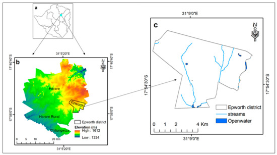
Figure 1.
Study site—Epworth district of the Harare Metropolitan Province. (a) Zimbabwe provincial boundaries including the Harare Metropolitan Province. (b) Elevation and district boundaries of the Harare Metropolitan Province. (c) Epworth district with hydrological network, retrieved from OSM data (OSM-Geofabric).
The Harare Metropolitan area is located on the Highveld at an elevation between 1455 m and 1556 m a.s.l., with a general topography characterized by undulating to slightly rolling terrain in the plateau areas. Annual precipitation in Harare Metropolitan Province varies between 470 mm and 1350 mm, falling mainly during the four months of the rainy season between mid-November to mid-March. Daily temperature ranges between 13 °C and 28 °C during the hot-dry season (September to mid-November) and low temperature averages between 7 °C and 20 °C are experienced during the cool-dry season (mid-May to August) [22]. Dominating soil types in Epworth district are the widely spread Paraferrallitic soils (coarse grained) covering the high-altitude areas and clayey Fersiallistic soils developed predominantly from dolerite in the central plateau [75]. Both soil types are largely influenced by nutrient loss through moderately to strongly occurring leaching processes [75,76].
2.2. Urban Land Use Change Modelling Using CA–Markov
The CA–Markov analysis was adopted to predict land use future scenarios. The CA–Markov model is embedded into the IDRISI software (Clarks Lab), an image processing software useful for improved digital image display and spatial analysis [77]. The Markov chain analysis describes the probability of LULC changes from one state to another at given times t1 and t2 by developing a transition probability [49,78,79]. The Markov chain model simulates land use changes and generates a transition probability matrix, which indicates the probability of each LULC to change from one state to another, and this is obtained by cross tabulation of the earlier and later LULC maps. The proportional changes become the transition probability, indicating that each land use class will change to other categories using Equation (2). The conditional suitability maps are produced and display the probability that each land use category might be found at each pixel, with values standardized between 0 and 255 [9,42,80,81,82]. The transition probability of converting the current state of a system to another state in the next time step is determined using the mathematical expression Equation (1) [80,83]:
where Pij is the probability from state i to state j and Pn is the state probability of any time. Equation (1) must satisfy the following conditions:
0 ≤ Pij ≤ 1 (i, j = 1, 2, 3………, n)
These steps are performed to obtain the Markov chain model’s primary matrix and the matrix of the transition probability (Pij). The Markov prediction model is expressed as:
where Pn refers to the state probability of any time and P(0) stands for the primary matrix. High transitions have probabilities near 1, while low transitions attract probabilities near 0 [80,84].
The Markov chain probabilities of change represent all multi-directional LULC changes between land use classes [82]. The Markov chains were selected as a result of their simplicity, robustness and capability in mapping LULC transitions in complex urban areas [9,81]. Despite forecasting transition probabilities per land use category and their growth trends, the major limitation of the Markov chain model is its inability to simulate the spatial distribution of each land use category’s occurrence [42,79,82]. Due to the heterogeneity of urban systems and structures, historical information is essential for a better understanding and interpretation of simulated future spatial trends [19]. The subsequent limitations of the Markov chains can be addressed by combining their outputs with other models that have open structures, including the Cellular Automata (CA), Multi-Layer Perceptron (MLP) and the Stochastic Choice [77,84]. In the present study, we integrated the Cellular Automata (CA) into the Markov chain approach to address the spatiality limitations of the Markov chain model and the probable spatial transitions occurring in the study area over the given time [40,47,54,81].
The CA have high spatial resolution and computational efficiency, enabling the prediction of future urban growth trends based on the supposition that the state of each cell at the present time depends on the previous state of cells within the neighbourhood [46,85,86]. Thus, the CA models are based on four major attributes, which include the cell, the state, the neighbourhood, and the transition rule [47,87]. The cell element of the CA signifies spatial shapes and sizes on the ground, while real characteristics of the area (land use) at a discrete time, represented as grid cells, show the state [47,48,87]. The neighbourhood cells are the immediate adjacent cells that form the kernel, and the transition rules theoretically code for the transformation from one cell state to another state resulting from the changes in neighbouring cells at a discrete time and state [39,47]. Despite being a powerful and simple tool in modelling urban growth patterns, the CA models have a limited capability for quantifying aspects, and the simulation processes do not include urban growth driving forces [50,51].
The CA–Markov modules embedded in the IDRISI GIS software were used to simulate LULC distribution patterns for the year 2018 and to predict future LULC for the years 2034 and 2050. Primarily, the simulation phase of the 2018 LULC scenarios applied the Markov chain to generate a transition probability matrix, and transition suitability images between 1990 and 2008 using the LULC maps of the same period were generated using support vector machines (SVMs) by Marondedze and Schütt [15]. A proportional error of 15% was set during the modelling of the transition probability matrix [77]. The Markov chain analysis outputs from 1990 and 2008 formed the basis of input parameters for the probable simulation of LULC spatial characteristics and their occurrence in the CA for the prediction of LULC patterns for 2018 (Figure 2). The contiguity filter specified the spatial characteristics applied by the CA modelling approach [40,77]. For this study, a contiguity filter of 5*5 pixels was applied to define the kernel due to higher spatial characterization when applied to determine the occurrence or position of the simulated LULC category compared to 3*3 or 7*7 [88,89].
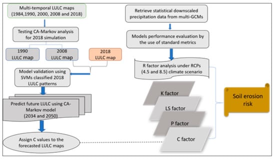
Figure 2.
Conceptual framework for the prediction of future LULC and soil erosion risk for Epworth district. LULC: land use and land cover. RCPs: representative concentration pathways, GCMs: global circulation models.
The spatiality characteristics in the CA approach were developed in a spatially explicit weighting that enabled the transformation of single and random grid cells in areas closer to the existing and widely spread land use [54,90]. This is further simplified by assuming that a pixel that is near one specific land cover class is more likely to be transformed to that category than pixels farther apart [78]. This assumption was used to initially test the predictive capability of the CA–Markov model set of the LULC distribution patterns for 2018. The cross validation of the 2018 simulated LULC patterns was performed applying the LULC patterns as provided by a support vector machines (SVMs) supervised classification map [15]. Finally, the CA–Markov techniques were applied between the LULC patterns of 2000 and 2018 for the prediction of future LULC distribution patterns for 2034, whilst the LULC distribution patterns of 1984 and 2018 were applied for the future prediction of 2050 LULC patterns. A 5*5 contiguity filter was applied for the prediction of future LULC patterns for the years 2034 and 2050.
2.3. Cellular Automata–Markov Chain Validation
The simulated LULC distribution patterns for 2018 were compared with the SVMs classified map for the same year to test the level of agreement. A two-phase validation approach was performed, which includes visual inspection and quantitative evaluation [9,91]. Visual inspection allowed close comparison and the agreement assessment between the simulated 2018 LULC map and the SVMs supervised classification LULC map. The kappa index of agreement (KIA) was used to assess the prediction accuracy for the 2018 actual map and the simulated LULC maps [54,91,92]. In general, kappa is referred to as a member of a family of indices with the properties (a) kappa = 1, when the level of agreement is perfect, and (b) kappa = 0, when the observed agreement is equal to the expected proportion due to chance [18]. Considering the model validity and performance in predicting LULC patterns for 2018, the LULC patterns for 2000–2018 and 1984–2018 were used in the prediction of 2034 and 2050 LULC spatial trends in the CA–Markov model. This introduces kappa indices to assess the performance and agreement of the model: the traditional kappa, which measures a simulation’s ability to attain perfect classification, that is, the closer to 1 the values are, the higher the level of agreement (Kstandard); the improved general kappa statistic, which is described as kappa for no ability (Kno); followed by the sophisticated kappa statistics (Kquantity and Klocation) used for distinguishing placement accuracies in both the quantity and location [54,92]. The Kno denotes the proportion classified correctly relative to the expected proportion classified correctly by a simulation without the ability to accurately specify quantity or location [18,92].
2.4. Predicting Future Soil Erosion Risk
The empirical RUSLE model was used to predict the spatially differentiated risk of long-term average annual soil loss. The selection of the empirical RUSLE model to assess future potential soil erosion risk considered the availability of data, robustness, complexity of the landscape and calibration [93,94]. The RUSLE model is widely used and a powerful tool to quantitatively assess spatial interactions of land use, topographic characteristics, climate, and soil characters in order to predict the spatial distribution of soil erosion [31,34,95,96,97]. The wide use of the empirical RUSLE model is based on its simplicity and easy accessibility of data compared to complex physical models [1,98]. Unlike other physical and process-based soil erosion models, the stochastic RUSLE model does not address soil deposition but mainly displays areas of sheet and rill erosion processes [98], allowing land managers to direct limited resources for landscape management [99]. The estimation of spatial soil erosion risk by the RUSLE model makes use of the factors soil erodibility (K), rainfall erosivity (R), slope length and steepness (LS), land cover and management (C) and the support practices (P) [97]. The RUSLE model calculates the risk of long-term average annual soil loss rates by multiplying the different factors:
where A: annual average soil loss (t ha−1 yr−1), R: rainfall erosivity factor (MJ mm ha−1 h−1 yr−1), K: soil erodibility factor (t ha h ha−1 MJ−1 mm−1), C: cover-management factor (dimensionless), LS: slope length and slope steepness factor (dimensionless) and P: support practices factor (dimensionless).
The RUSLE factors harmonized at 30 × 30 m spatial resolution for the compatibility of data from different sources [100] are multiplied to predict the soil erosion risk for the district using raster calculator in ArcGIS® 10.2. The computation of the RUSLE model integrates remote sensing and GIS techniques to analyse factors and geostatistics for the graphical interpretation [97,101].
Soil erodibility factor (K). The soil erodibility factor (K) represents the susceptibility of the soil to detachment due to rainfall erosivity (R) [97]. The soil erodibility factor varies corresponding to soil properties such as soil texture, type and size of aggregates, shear strength, soil structure, infiltration capacity, bulk density, soil depth, organic matter and other chemical constituents [97,102]. Based on the RUSLE model, the estimated K-factor values range between 0 and 1, indicating the degree of soils’ susceptibility to erosion [97]. Thus, soils being highly susceptible to erosion have soil erodibility values near 1, whereas the corresponding values close to 0 designate the resistive ability of a particular soil to erosion processes [103]. For this research, available data for the computation of the K factor were retrieved from ISRIC (International Soil Reference Information Centre), available at 250 m spatial resolution [104]. The estimation of the K factor was performed using the equation by Sharpley and Williams [105], which excludes soil structure and profile permeability due to the unavailability of experimental based information.
Slope length and slope steepness factor (LS). The RUSLE model considers the effects of topography on soil erosion, including slope length (L) and slope steepness (S). The Shuttle Radar Topography Mission (SRTM) digital elevation model (DEM) with a spatial resolution of 30 × 30 m (https://earthexplorer.usgs.gov/SRTM1Arc; accessed on 19 September 2020) was used for the computation of the LS factor using the Hydrology module (field-based), embedded in SAGA 2.3 software [106,107].
Land cover and management factor (C) and support practice factor (P). The land cover and management factor of the RUSLE model represents the effects of vegetation cover on soil erosion rates [97]. The C factor ranges from 0 for high-density vegetation to 1 for barren land; bare land is frequently used as the reference land use for C factor calibration [108,109]. The vegetation cover plays a vital role in dissipating raindrop energy before reaching the surface, thereby reducing the harsh effects posed by raindrop impact on the soil surface [101,108]. The C factor values in Table 1 result from the weighted field-based observations, and additional biophysical characterizations were adopted [23]. The support practice factor (P) was assigned to be 1, corresponding to the lack of support practice all over the study area [23].

Table 1.
The weighted C factor values.
Rainfall erosivity factor (R) estimation: The R factor describes the soil loss potential triggered by rainfall [97,102,110]. As such, the analysis of the spatial distribution of rainfall erosivity was computed following the empirical relations developed by El-Swaify et al., [111] Equation (6), as cited [34,112],
where R = rainfall erosivity factor (MJ mm ha−1 h−1 yr−1), and M = mean annual rainfall.
The further analysis highlights the likely potential effects of climate change on the R factor. The representative concentration pathway (RCP) 4.5 and 8.5 climate scenarios projected by multiple general circulation models (GCMs) were selected for the assessment of future climate change, primarily variations in precipitation magnitudes on soil erosion risk (downloaded from https://earthobservatory.nasa.gov/images/86027/; accessed on 2 October 2020). These climate change scenarios constitute a set of greenhouse gas concentration and emission pathways to facilitate decision and policy makers in the crafting of sustainable climate policies due to their plausibility [57,68]. To predict future rainfall erosivity, future RCP 4.5 and 8.5 climate scenarios proposed by the Intergovernmental Panel on Climate Change [26] were applied (Table 2). Annual rainfall, as required for Equation (6), was the sum of mean monthly rainfall data retrieved from the NASA Exchange Global Daily Downscaled Projections (NEX-GDDP), as listed in Table 2, which was statistically downscaled to a 0.25° by 0.25° spatial resolution [62,113]. The NEX-GDDP general circulation models grid point data locations do not match with the Harare Meteorological gauging points, as the spatial coverage of station data is not uniform; to cope with the varying spatial resolutions, annual averages were interpolated using the inverse distance-weighted methods [2].
Table 2.
Global circulation models (GCMs) used for data retrieval.
General circulation models’ performance was assessed, comparing their average annual rainfall data as provided per grid cell between 1980 and 2005 with the observed data from Harare gauging stations. This evaluation was processed by applying the interpolated GCMs average rainfall data from six available grid points within the Harare Metropolitan Province in parallel with observed average precipitation from the Harare Meteorological stations (Table 3) using the standard statistical metrics [114]. The evaluation of the GCMs performance was assessed using the standard metrics to outweigh GCMs that are not representative: the coefficient of determination (R2), relative root mean square error (rRMSE) (%), correlation coefficient (r), and index of agreement (d) [63,115,116]. With values ranging between 0 and 1, the lower the values of the rRMSE, the better the model’s performance, while the higher the value for R2, the better the goodness of fit of the model [115,116,117]. For the index of agreement (d), the closer values are to 1, the better they document the increasing goodness of the fit of the model, ascertaining that there is good agreement between the simulated and observed annual precipitation [63,118,119].
Table 3.
Location of Harare Metropolitan Province gauging stations.
Separate runs of the GCMs ensemble averages from 2019 to 2034 and 2035 to 2050 were used for the assessment of climate variability and its impact on future soil erosion risk under RCP4.5 and RCP8.5 climate scenarios. Estimations of future climate change scenarios from single GCMs relay limited information required for the direct calculation of the R factor [120,121]. Therefore, the application of multi-GCM ensemble averages decreases individual model errors and provides more robust predictions for future climate change [61,63,64,122,123]. Accordingly, empirical relations were used between monthly and annual precipitation in order to analyse GCM outputs relative to R factor changes [120]. Thus, long-term model ensemble averages were analysed for trends in rainfall erosivity factor (R) using suitable empirical relations [97,121,124].
3. Results
3.1. Land Use Land Cover Changes
The LULC maps (1990–2008, 2000–2018 and 1984–2018) generated by supervised classification applying SVMs [15] were used to simulate LULC distribution patterns for 2018; simultaneously, they were used as the reference for the simulation accuracy and to forecast future land use for 2034 and 2050 (Figure 3). The adopted supervised classification maps of the years 1984–2018 [15] show seven distinct classes (Table 4). The overall classification of each LULC map for 1984, 1990, 2000, 2008 and 2018 was estimated to be 90.1, 85.1, 88.9, 87.6 and 89.7%, respectively. The overall Kappa coefficient values produced were 0.87, 0.82, 0.86, 0.85 and 0.87 [15]. The data reveal that spatial LULC patterns will significantly change during the forecasted periods, indicating that the expansion of the built-up areas will be at the expense of green spaces and croplands (Figure 3). The built-up areas will continue to grow towards the peripheries and into the southward direction of the Epworth district (Figure 3).
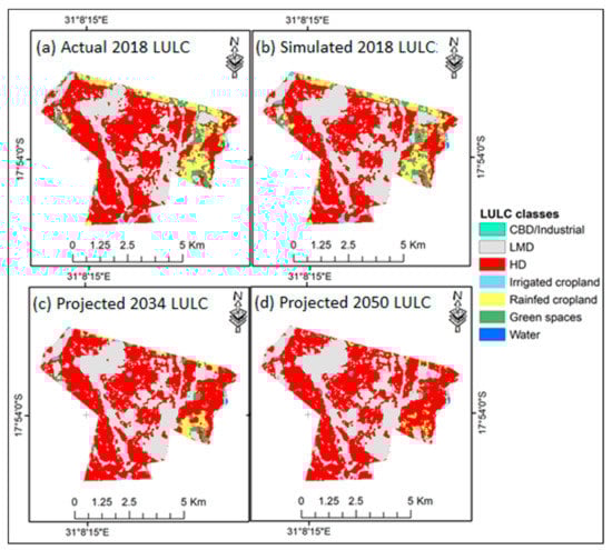
Figure 3.
Land use and land cover maps for Epworth district from the support vector machines supervised classification, simulated and predicted using the CA–Markov chain model: (a) actual 2018 supervised classification [15], (b) simulated 2018, (c) projected 2034 and (d) projected 2050. CBD: central business department, LMD: low–medium density, HD: high density.
Table 4.
Description of LULC classes for the study (source: [15]).
Comparison of LULC areas for 2018, resulting from the supervised classification applying SVMs, with 2018 simulated LULC classes shows that the land use land cover classes CBD/industrial, croplands, green spaces and water (Figure 3a,b) fit reasonably when comparing each class category, while slight differences between mapped and simulated distribution patterns occur for low–medium density and high-density residential areas (Figure 4). To summarize, for the period 2018 to 2050, the LULC class of CBD/industrial areas are estimated to remain stable, with an area expansion of +/−0.5–0.6% (Table 5). The spatial distribution of the LULC classes CBD/industrial area, water and irrigated croplands as projected for 2034 and 2050 widely correspond to those as mapped for 2018 (Figure 4). For both projected scenarios 2034 and 2050, the low–medium residential areas are predicted to increase slightly from 11.1 km2 to approximately 11.9 km2 between 2018 and 2034 and up to 12.3 km2 in scenario 2050. Similarly, high-density residential areas are predicted to increase from 18.6 km2 to 20.3 km2 between 2018 and 2034, and to reach 22.4 km2 in 2050 (Figure 4).
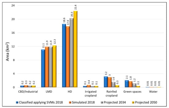
Figure 4.
The spatial area extent of different land use land cover classes for Epworth district: the depiction shows the variation between actual 2018 support vector machines (SVMs) supervised classification and the simulated 2018 LULC classes, including the predicted area LULC class extent for 2034 and 2050. CBD: central business department, LMD: low–medium density, HD: high density.
Table 5.
Relative proportions of LULC classes by area extent (km2) and percentage (%) for the adapted 2018 and the projected 2034 and 2050.
Low–medium-density residential areas (LMD) are predicted to increase in coverage from 31.5% to 34.8% between 2018 and 2050, while high-density (HD) residential areas are predicted to increase in coverage from 52.6% to 63.3% between 2018 and 2050 (Table 5). During the period 2018–2050, the spatial distribution of croplands is predicted to decrease from 9.5% to 1.1% of the total Epworth district area, while green spaces will shrink from 5.8% to 0.1%, largely due to the spatial expansion of built-up areas.
The summary of the probability matrix for major LULC conversions that occurred in Epworth district between 1990 and 2008 is documented in Table 6. The probability of change for CBD/industrial areas to remain CBD/industrial areas between 1990 and 2008 was 96.5%, displaying that built-up areas widely remained stable and will remain stable (Table 6). In contrast, irrigated croplands had a probability of change of 19.1%, that is, to remain irrigated cropland between 1990 and 2008, while the probability of change of irrigated cropland to rainfed cropland was 7.3% and to high-density residential areas was 47.2%. For green spaces, the probability to remain as green spaces between 1990 and 2008 was as low as 18.3%, while the probability of the change of green spaces to low–medium-density residential areas was 18.5%, to high-density residential areas was 40.8% and to croplands was 13.9% (Table 6).
Table 6.
Markov chain transition probability matrix from LULC maps between 1990 and 2008.
The Markov chain transition probability matrix computed LULC maps between 2000 and 2018 for the prediction of 2034 future LULC distribution patterns (Table 7), which indicates that in 2018 the built-up area classes have a probability of more than 95% to remain as built-up areas in the future, documenting a stable distribution at least until 2034. For the irrigated croplands, a probability of 10.1% is indicated to remain as irrigated croplands until 2034, while at the same time 24.1% of the irrigated croplands have a probability to be converted into low–medium-density residential areas, and even 40.4% of the irrigated croplands underly a probability to be converted into high-density residential areas until 2034. For rainfed cropland, a probability of 33% is indicated to remain as rainfed cropland until 2034, while there is a 42.8% probability that rainfed cropland will be converted into high-density residential areas. There is a probability of 14.1% that rainfed cropland will be converted into low–medium-density residential areas by 2034, while at the same time there is an 8.3% probability that the rainfed croplands will be converted into green spaces. Similarly, green spaces have a probability of 24.7% to remain as green spaces until 2034, while for the same period, green spaces have a 30.6% probability to be converted into high-density residential areas, and a 16.1% probability to be converted into low–medium-density residential areas.
Table 7.
Markov chain transition probability matrix from LULC maps between 2000 and 2018.
Based on the period 1984–2018, the transition probability matrix for the prediction of 2050 LULC distribution patterns was calculated (Table 8). The results indicate that built-up areas have probabilities higher than 90% to remain as built-up areas until 2050. In contrast, irrigated croplands have only a probability of 15% to remain as irrigated croplands until 2050, while they simultaneously have a probability of 41% to be transformed into high-density residential areas and a 21.4% probability to be transformed into low–medium-density residential areas. The rainfed croplands have a probability of 22.3% to remain as rainfed cropland until 2050; simultaneously, a 5.1% probability occurs that rainfed cropland will be transformed into irrigated croplands, a 5.3% probability occurs that rainfed cropland will be transformed into green spaces and a 42.5% probability occurs that rainfed cropland will be transformed into high-density residential areas.
Table 8.
Markov chain transition probability matrix from LULC maps between 1984 and 2018.
3.2. Validation of CA–Markov Model
A two-stage model validation approach was performed, including the visual inspection and quantitative assessment. The visual inspection shows that there is close agreement between the 2018 LULC distribution patterns derived from the support vector machines supervised classification (actual) and the 2018 LULC patterns simulated using the CA–Markov model (Figure 3). The computed kappa statistics recorded a kappa for a no ability Kno of 0.8893, a kappa for quantity accuracy KlocationStrata of 0.8943, a traditional kappa Kstandard of 0.9044 and a kappa for location accuracy Klocation of 0.925. To summarize, the kappa index of agreement values indicates that there is good agreement between the actual and simulated 2018 LULC maps. Therefore, the model can be applied with a high confidence in its reliability to forecast LULC maps for 2034 and 2050 (Table 9).
Table 9.
Kappa indices computed between the actual and simulated 2018 LULC maps.
3.3. Future Climate Data Analysis
The predicted meteorological data, as provided by the global circulation model ensemble, show slightly diverging data in terms of precipitation regimes by the different climate scenarios for the observation period 2019–2050. Comparing annual rainfall predictions as provided by the RCP8.5 climate scenario and RCP4.5 climate scenario (Figure 5) indicates similar trends with varying magnitude. In climate scenario RCP4.5, the predicted annual rainfall oscillates with an overall decrease until 2050; the maximum predicted annual precipitation reaches around 950 mm in the years 2022, 2025, 2029 and 2031 and then decreases, reaching 855 mm in 2041 and around 785 mm in 2045 and 2050 (Figure 5). Underlying the same overall decline in precipitation, the minimum annual precipitation as predicted by climate scenario RCP4.5 varies between 814 mm in 2027 and 770–780 mm in 2034 and 2046. In climate scenario RCP8.5, the predicted annual rainfall also oscillates but does not show a distinct decrease during the forecasted period until 2050, as shown by the outcomes of RCP8.5. Maximum predicted annual precipitation varies between 800 and 900 mm and minimum predicted annual precipitation varies between 705 and 740 mm. The years of maximum predicted annual precipitation in RCP4.5 and RCP8.5 widely concur, but offsets can also be repeatedly observed (Figure 5).
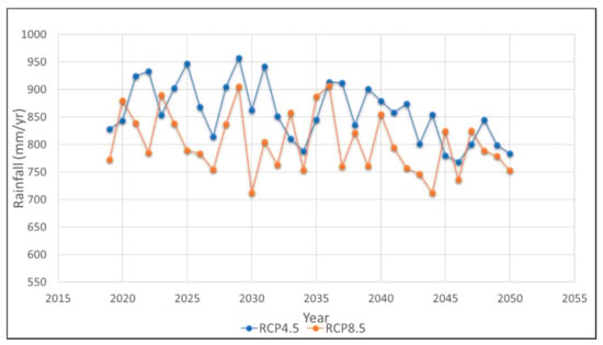
Figure 5.
Annual rainfall variations for Epworth district, 2019–2050, based on global circulation model ensemble climate scenarios RCP4.5 and RCP8.5.
3.4. Model Performance Evaluation
The performance evaluation carried out for each of the 15 statistically downscaled global circulation models’ outcomes with in situ historical observations from the Harare gauging stations varied, as displayed in Table 10. The global circulation model performance evaluations show that fourteen GCMs (ACCESS1-0, BNU-ESM, CanESM2, CNRM-BGC, GFDL-ESM2G, GFDL-ESM2M, MIROC-ESM, MIROC5, MPI-ESM-LR, MPI-ESM-MR and NorESM1-M, CCSM4, IPSL-CM5A-LR, MIROC-ESM-CHEM) have sufficient performance when evaluated against observations (d > 0.7, r > 0.7 and R2 > 0.5). The least successful performance in terms of accuracy when evaluating historical observations and global circulation models’ average precipitation data was observed for MRI-CGCM3 (R2 < 0.5), but the results show that the model has a strong positive correlation (r > 0.7) with a high index of agreement (d > 0.7), and an rRMSE below 20% (Table 10). As such, there is confidence to apply the GCM data for future soil erosion risk estimation for Epworth district (Table 10).
Table 10.
The GCMs’ performance evaluation against the observed precipitation dataset from 1980 to 2005.
3.5. RUSLE Model Factor Maps
To be able to later assess the impact of future climate change on the future long-term potential soil erosion risk for Epworth district, the analysis of future predicted precipitation was split into two time intervals, 2019–2034 and 2035–2050; applying the RCP4.5 climate scenario between 2019 and 2034, annual rainfall averages 886 mm, and for the time interval 2035–2050, annual rainfall averages 839 mm; applying the RCP8.5 climate scenario between 2019 and 2034, annual rainfall averages 827 mm, and for the time interval 2035–2050 annual rainfall averages 799 mm. For the time period 2019–2034, rainfall erosivity factor (R) values, as derived from RCP4.5 model ensemble, are on average between 333 and 338 MJ mm ha−1 h−1 yr−1 and significantly exceed the values of the R factor based on the RCP8.5 model ensemble of 318–324 MJ mm ha−1 h−1 yr−1 (Figure 6). For the period 2035–2050, the R factor calculated on the basis of the RCP4.5 climate scenario varies between 321 and 328 MJ mm ha−1 h−1 yr−1, again exceeding the R factor derived from the RCP8.5 model ensemble, which varies between 313 and 318 MJ mm ha−1 h−1 yr−1. The variation in the R factor values dictates the temporal variation in annual rainfall for different climate scenarios. High R factor values were recorded from the RCP4.5 model ensemble averages for both future periods considered, the highest R factor being predicted for the period 2019–2034.
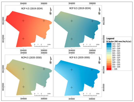
Figure 6.
The rainfall erosivity factors (R) for Epworth district for the time periods: (Top right) 2019–2034 (RCP4.5); (Top left) 2019–2034 (RCP8.5); (Bottom right) 2035–2050 (RCP4.5); and (Bottom left) 2035–2050 (RCP8.5).
The soil texture in Epworth district corresponds largely to sand, sandy loam and clayey loam; only along the alluvial plains do predominantly sandy loams occur. Correspondingly, soil erodibility factor values (K) range between 0.06 and 0.09 (Figure 7b). The topography of Epworth district is undulating to gently rolling, with steep sloping areas along the river banks and at the intersections of tributary channels into the major receiving streams. Related topographic factor values (LS) range from 0 in the plateau areas up to approximately 22 on the steep sloping areas (Figure 7a). The width of the weighted land cover and management factor values (C) range between 0 and 0.239, with different distribution patterns in 2034 and 2050 (Figure 7c,d). Major differences in land cover and management relate to shifts in land use over time, as predicted by the CA–Markov model (Figure 3). Due to the lack of support practices in the study area, the support practice factor values (P) are set as 1.
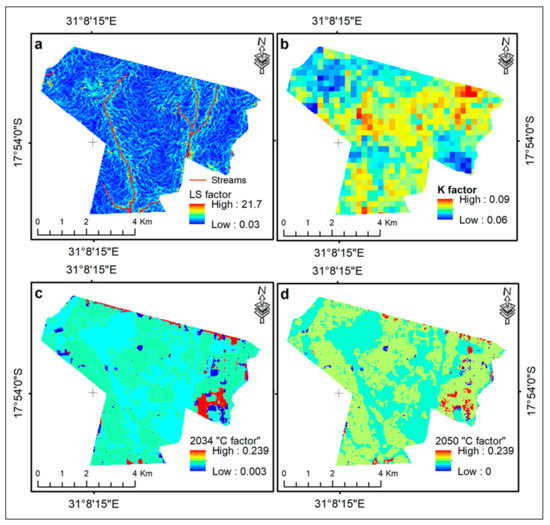
Figure 7.
RUSLE input factors for modelling potential soil erosion risk for Epworth district. (a) Topographic factor (LS); (b) soil erodibility factor (K); (c) the crop cover and management factor (C) for 2034; (d) the crop cover and management factor (C) for 2050.
3.6. Potential Soil Erosion Risk
Potential soil erosion risk mapping was performed independently for the years 2034 and 2050 as selected time slices, considering the two climate scenarios RCP4.5 and RCP8.5. The predicted average soil erosion risk, applying precipitation data as provided by RCP4.5 for the period 2019–2034, totals 1.2 t ha−1 yr−1 for 2034 and 1.1 t ha−1 yr−1 for the period 2035–2050. Applying the R factor based on the annual precipitation data, as provided by climate scenario RCP8.5, the predicted average potential soil erosion risk amounts to 1.1 t ha−1 yr−1 in 2034 and 1.0 t ha−1 yr−1 in 2050. The estimated soil loss rate for the climate scenario RCP4.5 in 2034 varies between 0 and 69.3 t ha−1 yr−1 and 0 and 48.9 t ha−1 yr−1 in 2050. Applying the R factor based on the annual precipitation data, as provided by climate scenario RCP8.5, soil loss rates ranged between 0 and 62.4 t ha−1 yr−1 in 2034 and 0 and 42.3 t ha−1 yr−1 in 2050. Future potential soil erosion risk predictions for climate scenarios RCP4.5 and RCP8.5 were significantly different (p < 0.05) for each time interval, 2034 and 2050, highlighting that the presented changes can be attributed to various predicted factors, including land use and rainfall erosivity changes.
High potential soil erosion risk areas are predicted for the south-eastern periphery of Epworth district and along the tributaries, as well moving downwards in the south direction along the stream, as depicted in Figure 8. The predicted spatial patterns of potential soil erosion risk applying annual precipitation data, as provided by the RCP4.5 and RCP8.5 climate scenarios for the time slices 2034 and 2050, reveal in all cases high potential soil erosion risk along the flanks of the major rivers and along the flanks of steep tributaries (Figure 8). The displayed potential soil erosion risk maps in Figure 8 reveal that the predicted decrease in the R factor in the long term, corresponding to decrease in annual rainfall averages, reduces soil erosion processes, which simultaneously is on the rise in some localized parts of the district, and this is purportedly triggered by land use changes. Environmental characters, predominantly topography and soil properties (Figure 7), control the overall vulnerability of the area to soil erosion, finally displayed as potential soil erosion risk, including rainfall and land use.
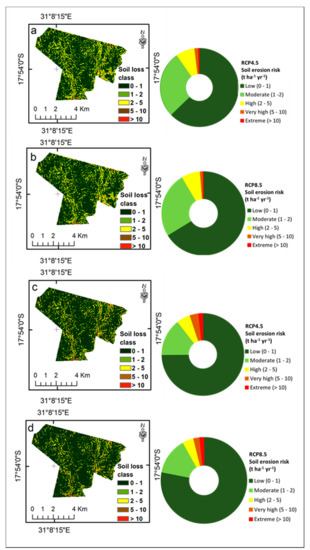
Figure 8.
Predicted spatio-temporal potential soil erosion risk for Epworth district. (a) Potential soil erosion risk for 2034 applying R factors based on RCP4.5; (b) potential soil erosion risk for 2034 applying R factors based on RCP8.5; (c) potential soil erosion risk for 2050 applying R factors based on RCP4.5; and (d) potential soil erosion risk for 2050 applying R factors based on RCP8.5.
The area-wide potential soil erosion risk predicted for the year 2034, applying R factors derived from the RCP4.5 climate scenario, indicates that 62.0% of the Epworth district will be exposed to low potential soil erosion risk and 27.9% to moderate potential soil erosion risk, while 8.1% will be exposed to high potential soil erosion risk and 2.0% to very high and extreme potential soil erosion risk (Table 11). The predicted results evidently show that there is an extensive distribution of areas of low potential soil erosion risk across the district, while high potential soil erosion risk is predicted predominantly along the channel networks. Applying R factors from the same climate scenario, RCP4.5, for the year 2050, approximately 74.3% of the entire district will be exposed to low potential soil erosion risk, 14.7% will be exposed to moderate potential soil erosion risk, 5.6% will be exposed to high potential soil erosion risk and 5.4% to very high and extreme potential soil erosion risk. The area-wide proportion of low potential soil erosion risk extended extensively across the entire district in 2050, attributed to the decline in the average rainfall erosivity in climate scenario RCP4.5. Applying R factors based on the RCP8.5 climate scenario in the year 2034, about 66.7% of the Epworth district is predicted to be exposed to low potential soil erosion risk, 24.6% to moderate potential soil erosion risk, 7.4% to high potential soil erosion risk and 1.3% to very high and extreme potential soil erosion risk (Table 11). Furthermore, for the year 2050, based on RCP8.5 climate scenario, the predicted area of Epworth district exposed to low potential soil erosion risk will be 77.7%, 14.1% will be exposed to moderate potential soil erosion risk, 4.6% to high potential soil erosion risk and 3.6% of the entire district will be exposed to very high and extreme potential soil erosion risk (Table 11). Applying climate scenario RCP8.5, similar to the application of climate scenario RCP4.5, high-intensity potential soil erosion is predicted predominantly along channel networks and predominates in the southern area of Epworth district (Figure 8).
Table 11.
Predicted proportion of the spatial area of Epworth district exposed to potential soil erosion risk.
The average area-wide potential soil erosion risk in Epworth district predicted for the time slices 2034 and 2050 shows extended areas exposed to low potential soil erosion rates between 0 and 1 t ha−1 yr−1, considering annual precipitation as provided by the RCP8.5 climate scenario. In contrast, the average area-wide potential soil erosion risk predicted for the time slices 2034 and 2050, considering annual precipitation as provided by RCP4.5 climate scenario, distinctively exposes a smaller area to low soil loss rates between 0 and 1 t ha−1 yr−1 compared to the respective predictions applying climate scenario RCP8.5. In relation to the study on the present-day soil erosion risk in Epworth district [23], the current area exposed to low soil erosion risk amounts to 59.5%; thus, it is predicted to distinctly increase in the future (Table 11). In contrast, currently 10% of the Epworth district is exposed to high soil erosion risk and up to 1.2% is exposed to very high and extreme soil erosion risk (Table 11). Correspondingly, it is expected that in the future, the areas in Epworth district exposed to high potential soil erosion risk with soil loss rates between 2 and 5 t ha−1 yr−1 will markedly decrease, and most likely will even halve by 2050. Furthermore, areas exposed to very high to extreme potential soil erosion risk with soil loss rates of more than 5 t ha−1 yr−1 will massively increase under future changes in land use and climate, while in 2034, under the RCP8.5 climate scenario, areas exposed to very high potential soil erosion risk will be widely stable compared to 2018 area coverage. By 2050, the spread of this category will double and might even triple when applying R-factors from the RCP4.5 climate scenario (Table 11). This development is even more distinctive when focusing on areas exposed to extreme potential soil erosion risk compared to the present-day situation until 2034, where areas exposed to extreme potential soil erosion risk will steadily increase by doubling the area extent when applying R-factors resulting from the RCP8.5 climate scenario, and up to 4 times the area extent when applying R-factors resulting from the RCP4.5 climate scenario. In 2050, areas exposed to extreme potential soil erosion risk will have increased by more than tenfold, independent of whether applying R-factors resulting from the RCP8.5 or RCP4.5 climate scenario. However, the total area exposed to extreme potential soil erosion risk remains small and predominantly will occur along the river banks (Table 11).
4. Discussion
The predicted CA–Markov model results reveal an increase in the spatio-temporal pattern of built-up area, with built-up area expected to cover over 95% in 2050 from an approximated total of 84.5% in 2018 (Figure 3, Table 5). The forecasted results indicate that green spaces and croplands will continue to decline at the expense of built-up area (Table 5). Thus, the transition probability matrices for different periods reveal the probability of each class (n) in the LULC maps changing in the next distinct period (tn+1) in respect of the surrounding cells [22,81]. These predictions of built-up area growth at the expense of green spaces and croplands in the Harare Metropolitan Province concur with the conversion rates predicted by Mushore et al. [9] using CA–Markov model analysis. The same analysis agrees with the predicted urban growth and the development of Irbid’s governorate of Jordan, with projected built-up area growth amounting to almost 65% in total area from an estimated 14.5% between 2015 and 2050, at the expense of vegetation and farmlands [55]. Therefore, such developments indicate the core principle of the CA models, which stipulates that the present state of development is a continuation of historical changes induced by the neighbourhood interactions [40,49,81]. This predicted expansion pattern is a result of the neighbourhood effect, which exhibits that the converted land use is next or close to the existing dominant land use, and predominantly built-up area exists for this scenario [39,47,49].
The predicted loss of green spaces and croplands may result in the detrimental loss of urban agricultural land and areas of aesthetic value to the ecosystem, which provide environmental protection. With the escalating socioeconomic woes and poverty in the city [70], the loss of urban agricultural land to urban development will leave many poorly resourced Epworth residents with detrimental food insecurities, threatening their livelihoods since many survive on market gardening and other urban farming activities [125,126]. The loss of green spaces also results in the reduction in vegetation cover and biomass which dissipates rainfall, reducing its direct impacts on the soil surface and facilitating percolation [101]. Further, with the current economic meltdown and population growth, the surge of urban built-up area predicted by the CA–Markov model can be justified; the Epworth district will be no exception in terms of absorbing more inhabitants from other spheres of the Harare Metropolitan Province. This push could be exacerbated by unaffordable rental charges and cost of living in other affluent suburbs of the Harare Metropolitan Province, resulting in further densification and overcrowding in Epworth district. However, due to excessive demand for shelter and anticipated population growth, the conversion of croplands and green spaces to a built-up area will intensify impervious surfaces across the district [15,127].
The GCM ensembles were used to quantify the hydrological impacts of climate change under different climate scenarios, RCP4.5 and RCP8.5, to obtain reliable projections [61,65,122,128]. Based on statistical metrics, the evaluation of the performance showed that fourteen GCMs (Table 10) have sufficient performance when evaluated with observations from Harare Metropolitan gauging stations (d > 0.7, r > 0.7 and R2 > 0.5), with the exception of MRI-CGCM3, observed to have the lowest determination coefficient of 0.47. This may suggest that the general circulation model could have other specific years that were not properly simulated [63]; however, the analysis shows that most GCMs displayed good simulation. Above all, the GCMs have an rRMSE below 20%, which is reasonably acceptable [116,117,129]. Further, coarse grid resolutions from GCMs make it difficult to match, with few in situ observations which are not uniformly distributed attributed to increases in spatial variation and uncertainty to clearly define local precipitation characteristics, therefore increasing the simulation bias [130,131,132].
For the RUSLE model, potential soil erosion risk maps were produced using the geostatistical ArcGIS package (raster calculator) to multiply the RUSLE factor maps (Figure 6 and Figure 7). The predicted potential soil erosion risk averaged at 1.2 t ha−1 yr−1 in 2034 and 1.1 t ha−1 yr−1 in 2050 for the RCP4.5 climate scenario, while 1.1 t ha−1 yr−1 and 1.0 t ha−1 yr−1 were the predicted averages for 2034 and 2050 for the RCP8.5 climate scenario. Meanwhile, studies on the influence of land use change or the impact of soil erosion risk on crop productivity indicated that a tolerable soil loss rate at 1 t ha−1 yr−1 was sustainable for the tropics [95,133,134,135]. Based on the slow rate of soil formation across the tropics, including Europe and America (<1 t ha−1 yr−1) [95,133,136,137], the sustainable soil loss tolerance at 1 t ha−1 yr−1 was considered across the entire Epworth district. The resulting arguments around the proposed 10 t ha−1 yr−1 as the estimated soil erosion tolerance threshold for tropical ecosystems showed that it was highly overestimated, considering threats to the landscape and impacts on crop productivity likely to occur at such a high risk threshold [138]. Furthermore, other studies indicated that average soil loss rates of 5 t ha−1 yr−1 may be sustainable soil loss rates in the tropics [139,140]. Nevertheless, an estimated 1 t ha−1 yr−1 soil loss threshold subsisted for the current study and the predicted area-wide averages were unsustainable in that they slightly surpassed the recommended soil loss threshold, except for the RCP8.5 climate scenario in 2050. However, the slight notable deviation from the 1 t ha−1 yr−1 sustainable threshold can be justified as the averages fall within the applicable tolerable range of c.a 1.4 t ha−1 yr−1 proposed for some parts of the tropics, including America and Europe [137]. Thus, the estimated soil loss tolerance threshold was used to describe a sustainable soil loss rate [141].
The integrated average annual precipitation between 2019 and 2034, based on the climate scenario RCP4.5 results, shows high average annual soil loss rates ranging between 0 and 69.3 t ha−1 yr−1 and 0 and 62.4 t ha−1 yr−1 for the RCP8.5 climate scenario in 2034. In contrast, applying average annual precipitation between 2035 and 2050, the R factor-based values show a decline in soil loss rates for the year 2050 in both climate scenarios ranging between 0 and 48.9 t ha−1 yr−1 for RCP4.5 and 0 and 42.3 t ha−1 yr−1 for RCP8.5. However, these results show a continuous declining trend of soil loss rates when compared with the baseline period that applied the R factor based on the average annual precipitation data derived from in situ observations between 1984 and 2000 for Epworth district, estimating high soil erosion risk with average annual soil loss rates between 0 and 92.8 t ha−1 yr−1 in 2000 [23]. In summary, the soil loss rates for both the RCP4.5 and RCP8.5 climate scenarios are observed to be decreasing in spatial coverage over the years 2034 and 2050. Regardless of the high rainfall erosivity predicted between 2019 and 2034 in comparison with soil loss rates estimated for the year 2000 [23], it is revealed that land use changes, including the shrinking of croplands and disturbed shrublands, predominantly reduce the soil loss impact due to increases in impervious surfaces across the Epworth district.
The increasing potential soil erosion risk predicted for Epworth district along the channel networks has been attributed to the steep slopes along the streams in combination with massive impervious surfaces, resulting in the accumulation of overland flow [142]. Correspondingly, high topographic factor values appear on valley flanks (Figure 7), exposing surfaces to severe runoff and flooding resulting from the increased slope inclination and reduced infiltration capacity [143,144]. Displayed soil loss rates exceeding 1 t ha−1 yr−1 for Epworth district will be considered unsustainable [95,137], and therefore, the need for sound policy implementation to avoid detrimental environmental damage. Such estimates, as indicated in Table 11, reveal that a larger proportion of the study area will be exposed to tolerable soil loss rates [95,133,134]. Nevertheless, there is a predicted increase in soil erosion risk in vulnerable areas, mainly downslope and low-lying areas along the flanks of the channel networks [23,142,145].
The study results predict that soil loss rates vary with precipitation and land use changes for all the climate scenarios. The results suggest that the soil erosion response with regard to climate change could be complex, as it varies with time and on a climate scenario basis [25]. Consequently, the proportion of area exposed to high potential soil erosion risk with average soil loss rates between 2 and 5 t ha−1 yr−1 will markedly decline and most likely will even halve by 2050, as opposed to the doubling and triplicating proportional areas exposed to very high and extreme potential soil erosion risk for both climate scenarios in 2050. This is linked with the increasing vulnerability to smaller proportional area occupied by sparse green spaces and bare areas along channel networks. Such increasing trends in potential soil erosion risks are primarily accelerated by concentrated overland flow resulting from reduced infiltration processes across the Epworth district [99,143,146]. This vulnerability and response to rainfall impact and runoff processes with regard to reduced spatial area exposed to direct soil displacement in 2050 underpins the effects of land use changes and sloping topography along the channel network [114,147].
The decreasing rainfall erosivity for both scenarios over time concurs with the future analysis that incorporated regional climate models (RCMs) by Hudson and Jones [130], in which they highlighted the likelihood of increasing consecutive dry days in southern Africa; however, with some increases in other parts of the region [148]. Additionally, interannual high rainfall intensity impact is relatively expressed as this would be masked in annual rainfall averages due to low rain-day frequency [148]. The contraction of the rainfall season was projected following the observed late onset and early rainfall cessation in sub-Saharan Africa, mostly in central Mozambique, large parts of Botswana and the northern and southern parts of Zimbabwe [148]. Such responses to climate change tally with the predicted decline in overall soil erosion risk in 2050, which, however, still require more robust regional analysis on precipitation uncertainties to global climate change [130,148,149]. Nevertheless, the use of model ensemble averages could have limited the impact of other predicted extreme rainfall events [61,65,122]. Such changes and manipulations of rainfall intensities could negatively impact the final soil erosion prediction outcome [150,151]. Furthermore, the use of coarse grid resolutions and numerical methods reduces models’ data independency, and therefore increases the bias and uncertainty range of the outcomes [61,122,123]. The empirical RUSLE model is also limited only to the predictive capacity of sheet, inter-rill and rill soil erosion processes spanning over long periods, as it is not an event-based model, which also does not consider gullying erosion processes [1,93,97,152,153]. Other data-driven processes integrated in the empirical RUSLE technique increase the uncertainty of future soil erosion risk due to varying data sources applied without rigorous quantification of their uncertainties and propagation [1,154].
Overall, high potential soil erosion risk displayed within the vicinity of Jacha river and tributaries extending from the north and southeast parts of the district draining southwards continue to increase, as predicted by the RUSLE model widely in 2050. This is attributed to the increasing sealed surface area and the sloping topography contributing to increased overland flow and surface runoff [143,155]. Taking into account human activities, previous studies reiterated that sand poaching activities along riverbanks are associated with heavy trucks ferrying sand to construction sites, contributing to high soil compaction on unpaved roads [23,24,142], reducing the infiltration capacity, and hence increasing surface runoff processes. For Epworth district, activities such as sand poaching and extraction along the riverbanks will be inevitable due to the predicted built-up area expansion and due to the fact that for many locals, informal activities provide employment for the sustenance of their livelihoods. Therefore, there is a need to implement sound policies and sustainable environmental management approaches in order to curb environmental damage and the future extinction of water bodies and their ecosystem services. Uncertainties exist in this study about policy amendments regarding the functionality of the Local Boards and Authorities in regulating developmental plans. This, in turn, will affect LULC changes in the Epworth district of the Harare Metropolitan Province. However, this was held constant in the prediction of future LULC distribution patterns for Epworth district.
5. Conclusions
The study uses LULC distribution patterns between 1990 and 2008 to apply a Markov chain model which allows the development of a transition probability matrix and suitability maps, and later defines the complex dynamic spatial patterns of urban area by the flexible Cellular Automatons. The validation of the simulated 2018 LULC distribution patterns and the actual 2018 LULC map displayed strong spatial agreement, both quantitatively and through visual inspection. The strong agreement and consistency of the LULC spatial patterns from the cross validation displayed the reliability and usability of the CA–Markov model to predict 2034 and 2050 future LULC distribution patterns for Epworth district. The predicted findings show a continuous increase in urban built-up area over the years 2034 and 2050 at the expense of croplands and perturbed green spaces, predominantly with the expansion of high-density residential areas towards Epworth district peripheries.
Further, future potential soil erosion risk was predicted for the years 2034 and 2050 using the RUSLE model, which integrated R factors based on the average annual precipitation between 2019 and 2034 and 2035 and 2050, as provided by climate scenarios RCP4.5 and RCP8.5. The goodness of fit measures highlighted that the general circulation models (GCMs) are useful for the assessment of future soil erosion risk, following the evaluation of GCMs performance with gauged observations, which showed a good performance, ascertaining their feasibility. As such, ensemble average outcomes from multiple GCMs under both the RCP4.5 and RCP8.5 climate scenarios were incorporated in the regional statistical relations equation to derive the rainfall erosivity factor for use in the RUSLE model.
Future trends in climate variability reveal that the projected high rainfall for the RCP4.5 climate scenario between 2019 and 2050 compared to the RCP8.5 climate scenario will contribute to high localized soil erosion risk in vulnerable areas, including perturbed green spaces, agricultural land and stream banks. High soil loss rates were predicted in 2034 for both climate scenarios RCP4.5 and RCP8.5, in comparison with low soil loss rates in 2050 for both climate scenarios, and this is largely attributable to the predicted dynamic land use changes resulting in the reduction in surface area exposed to soil erosion processes over time. The predicted results also indicate that average annual soil loss rates will approximately halve in 2050 from an estimated 0–93 t ha−1 yr−1 in 2000, independent of whether the RCP4.5 or RCP8.5 climate scenario is applied. Nevertheless, for 2050, increasing soil erosion risks have been predicted along the flanks of the drainage networks.
Overall, this study highlights the application of the CA–Markov model in combination with the RUSLE model to derive useful simulations for predicting future LULC and soil erosion risk. In addition, based on the stipulated IPCC policy recommendations from the Fifth Assessment Report (AR5), governments and policy makers need to implement sound climate policies in order to curtail and curb environmental degradation and landscape fragmentation at the local scale.
Author Contributions
All authors: conception of the paper; A.K.M.: data acquisition, data analysis, writing of the original draft; B.S.: supervision, writing—review and editing, funding acquisition. All authors have read and agreed to the published version of the manuscript.
Funding
This research was funded by the Deutscher Akademischer Austauschdienst—DAAD, and “The APC was funded by Freie Universität Berlin”.
Institutional Review Board Statement
Not Applicable.
Informed Consent Statement
Not applicable.
Data Availability Statement
SRTM DEM: (https://earthexplorer.usgs.gov/SRTM1Arc, accessed on 19 September 2020); GCMs: NASA Exchange Global Daily Downscaled Projections (NASA-GDDP) (Available online at https://earthobservatory.nasa.gov/images/86027/, accessed on 2 October 2020); In Situ datasets: obtained from Department of Meteorology in Harare on 01 July 2019; Global soil map and attributes retrieved from ISRIC (International Soil Reference Information Centre)—World Soil Information: (Available online at https://soilgrids.org, accessed: 17 July 2019). LULC maps: Marondedze and Schütt (2019) peer-reviewed article (doi:10.3390/land8100155).
Acknowledgments
The publication of this article was funded by Freie Universität Berlin. We thank our colleagues from Freie Universität Berlin for their valuable insights that greatly assisted this research work. We are grateful to the United States Geological Survey (USGS) for providing Landsat images and the terrain-corrected Shuttle Radar Topography Mission (SRTM) DEM. We extend our gratitude to the Department of Meteorology in Harare, Zimbabwe for providing rainfall data and NASA Earth Exchange Global Daily Downscaled Projections (NEX-GDDP) for providing statistically downscaled global climate models.
Conflicts of Interest
The authors declare no conflict of interest.
References
- Borrelli, P.; Robinson, D.A.; Panagos, P.; Lugato, E.; Yang, J.E.; Alewell, C.; Wuepper, D.; Montanarella, L.; Ballabio, C. Land Use and Climate Change Impacts on Global Soil Erosion by Water (2015–2070). Proc. Natl. Acad. Sci. USA 2020, 117, 21994–22001. [Google Scholar] [CrossRef]
- Mondal, A.; Khare, D.; Kundu, S.; Meena, P.K.; Mishra, P.K.; Shukla, R. Impact of Climate Change on Future Soil Erosion in Different Slope, Land Use, and Soil-Type Conditions in a Part of the Narmada River Basin, India. J. Hydrol. Eng. 2015, 20. [Google Scholar] [CrossRef]
- Karydas, C.G.; Sekuloska, T.; Silleos, G.N. Quantification and Site-Specification of the Support Practice Factor When Mapping Soil Erosion Risk Associated with Olive Plantations in the Mediterranean Island of Crete. Environ. Monit. Assess. 2009, 149, 19–28. [Google Scholar] [CrossRef] [PubMed]
- Islam, K.; Jashimuddin, M.; Nath, B.; Nath, T.K. Land Use Classification and Change Detection by Using Multi-Temporal Remotely Sensed Imagery: The Case of Chunati Wildlife Sanctuary, Bangladesh. Egypt. J. Remote Sens. Space Sci. 2018, 21, 37–47. [Google Scholar] [CrossRef]
- Lambin, E.F. Modelling and Monitoring Land-Cover Change Processes in Tropical Regions. Prog. Phys. Geogr. Earth Environ. 1997, 21, 375–393. [Google Scholar] [CrossRef]
- Brueckner, J.K.; Helsley, R.W. Sprawl and Blight. J. Urban Econ. 2011, 69, 205–213. [Google Scholar] [CrossRef]
- Jat, M.K.; Choudhary, M.; Saxena, A. Application of Geo-Spatial Techniques and Cellular Automata for Modelling Urban Growth of a Heterogeneous Urban Fringe. Egypt. J. Remote Sens. Space Sci. 2017, 20, 223–241. [Google Scholar] [CrossRef]
- Hegazy, I.R.; Kaloop, M.R. Monitoring Urban Growth and Land Use Change Detection with GIS and Remote Sensing Techniques in Daqahlia Governorate Egypt. Int. J. Sustain. Built Environ. 2015, 4, 117–124. [Google Scholar] [CrossRef]
- Mushore, T.D.; Odindi, J.; Dube, T.; Mutanga, O. Prediction of Future Urban Surface Temperatures Using Medium Resolution Satellite Data in Harare Metropolitan City, Zimbabwe. Build. Environ. 2017, 122, 397–410. [Google Scholar] [CrossRef]
- UN World Urbanization Prospects: The 2014 Revision, Highlights 2014. Available online: https://www.un.org/en/development/desa/publications/2014-revision-world-urbanization-prospects.html (accessed on 2 February 2021).
- UN World Urbanization Prospects: The 2011 Revision United Nations. 2012. Available online: https://www.un.org/en/development/desa/population/publications/pdf/urbanization/WUP2011_Report.pdf (accessed on 4 February 2021).
- World Economic Forum Global-Continent-Urban-Population-Urbanisation-Percent 2020. Available online: https://www.weforum.org/agenda/2020/11/global-continent-urban-population-urbanisation-percent/ (accessed on 24 March 2021).
- UN. Population Division Then & Now: Urban Population Worldwide 2020. Available online: https://population.un.org/wup/ (accessed on 24 March 2021).
- ZimStats (Zimbabwe National Statistics Agency) Census 2012: Preliminary Report. 2012. Available online: https://www.zimstat.co.zw/wp-content/uploads/publications/Population/population/census-2012-national-report.pdf (accessed on 14 October 2020).
- Marondedze, A.K.; Schütt, B. Dynamics of Land Use and Land Cover Changes in Harare, Zimbabwe: A Case Study on the Linkage between Drivers and the Axis of Urban Expansion. Land 2019, 8, 155. [Google Scholar] [CrossRef]
- Aburas, M.M.; Ho, Y.M.; Ramli, M.F.; Ash’aari, Z.H. The Simulation and Prediction of Spatio-Temporal Urban Growth Trends Using Cellular Automata Models: A Review. Int. J. Appl. Earth Obs. Geoinf. 2016, 52, 380–389. [Google Scholar] [CrossRef]
- Myers, G. African Cities: Alternative Visions of Urban Theory and Practice; Zed Books Ltd.: London, UK, 2011; ISBN 1780321333. [Google Scholar]
- Pontius, R.G. Quantification Error versus Location Error in Comparison of Categorical Maps. Photogramm. Eng. Remote Sens. 2000, 66, 1011–1016. [Google Scholar]
- Sudhira, H.S.; Ramachandra, T.V.; Jagadish, K.S. Urban Sprawl: Metrics, Dynamics and Modelling Using GIS. Int. J. Appl. Earth Obs. Geoinf. 2004, 5, 29–39. [Google Scholar] [CrossRef]
- Chalise, D.; Kumar, L.; Kristiansen, P. Land Degradation by Soil Erosion in Nepal: A Review. Soil Syst. 2019, 3, 12. [Google Scholar] [CrossRef]
- Shikangalah, R.; Paton, E.; Jetlsch, F.; Blaum, N. Quantification of Areal Extent of Soil Erosion in Dryland Urban Areas: An Example from Windhoek, Namibia. Cities Environ. (CATE) 2017, 10, 22. [Google Scholar]
- Kamusoko, C.; Gamba, J.; Murakami, H. Monitoring Urban Spatial Growth in Harare Metropolitan Province, Zimbabwe. Adv. Remote Sens. 2013, 02, 322–331. [Google Scholar] [CrossRef]
- Marondedze, A.K.; Schütt, B. Assessment of Soil Erosion Using the RUSLE Model for the Epworth District of the Harare Metropolitan Province, Zimbabwe. Sustainability 2020, 12, 8531. [Google Scholar] [CrossRef]
- USDA. NRCS Soil Quality—Urban Technical Note No. 1: Erosion and Sedimentation on Construction Sites 2000. Available online: http://www.aiswcd.org/wp-content/uploads/2013/04/u011.pdf (accessed on 18 May 2020).
- Pruski, F.F.; Nearing, M.A. Climate-Induced Changes in Erosion during the 21st Century for Eight U.S. Locations: Climate-Induced Changes in Erosion. Water Resour. Res. 2002, 38, 34-1–34-11. [Google Scholar] [CrossRef]
- IPCC, (Intergovernmental Panel on Climate Change). Climate Change 2014: Impacts, Adaptation, and Vulnerability. Contribution of Working Group II to the Fifth Assessment Report of the Intergovernmental Panel on Climate Change 2014. Available online: https://www.ipcc.ch/report/ar5/wg2/ (accessed on 15 February 2021).
- Gupta, S.; Kumar, S. Simulating Climate Change Impact on Soil Erosion Using RUSLE Model—A Case Study in a Watershed of Mid-Himalayan Landscape. J. Earth Syst. Sci. 2017, 126, 43. [Google Scholar] [CrossRef]
- Li, Z.; Fang, H. Impacts of Climate Change on Water Erosion: A Review. Earth-Sci. Rev. 2016, 163, 94–117. [Google Scholar] [CrossRef]
- Segura, C.; Sun, G.; McNulty, S.; Zhang, Y. Potential Impacts of Climate Change on Soil Erosion Vulnerability across the Conterminous United States. J. Soil Water Conserv. 2014, 69, 171–181. [Google Scholar] [CrossRef]
- Simonneaux, V.; Cheggour, A.; Deschamps, C.; Mouillot, F.; Cerdan, O.; Le Bissonnais, Y. Land Use and Climate Change Effects on Soil Erosion in a Semi-Arid Mountainous Watershed (High Atlas, Morocco). J. Arid Environ. 2015, 122, 64–75. [Google Scholar] [CrossRef]
- Feng, X.; Wang, Y.; Chen, L.; Fu, B.; Bai, G. Modeling Soil Erosion and Its Response to Land-Use Change in Hilly Catchments of the Chinese Loess Plateau. Geomorphology 2010, 118, 239–248. [Google Scholar] [CrossRef]
- Routschek, A.; Schmidt, J.; Kreienkamp, F. Impact of Climate Change on Soil Erosion—A High-Resolution Projection on Catchment Scale until 2100 in Saxony/Germany. CATENA 2014, 121, 99–109. [Google Scholar] [CrossRef]
- Makwara, E.C.; Gamira, D. About to Lose All the Soil in Zaka’s Ward 5, Zimbabwe: Rewards of Unsustainable Land Use. Eur. J. Sustain. Dev. 2012, 1, 457. [Google Scholar] [CrossRef][Green Version]
- Tundu, C.; Tumbare, M.J.; Kileshye Onema, J.-M. Sedimentation and Its Impacts/Effects on River System and Reservoir Water Quality: Case Study of Mazowe Catchment, Zimbabwe. Proc. Int. Assoc. Hydrol. Sci. 2018, 377, 57–66. [Google Scholar] [CrossRef]
- Whitlow, R. Soil Erosion and Conservation Policy in Zimbabwe. Land Use Policy 1988, 5, 419–433. [Google Scholar] [CrossRef]
- Mullan, D.; Favis-Mortlock, D.; Fealy, R. Addressing Key Limitations Associated with Modelling Soil Erosion under the Impacts of Future Climate Change. Agric. For. Meteorol. 2012, 156, 18–30. [Google Scholar] [CrossRef]
- Herold, M.; Goldstein, N.C.; Clarke, K.C. The Spatiotemporal Form of Urban Growth: Measurement, Analysis and Modeling. Remote Sens. Environ. 2003, 86, 286–302. [Google Scholar] [CrossRef]
- Tang, J.; Wang, L.; Yao, Z. Spatio-temporal Urban Landscape Change Analysis Using the Markov Chain Model and a Modified Genetic Algorithm. Int. J. Remote Sens. 2007, 28, 3255–3271. [Google Scholar] [CrossRef]
- Tang, J.; Di, L. Past and Future Trajectories of Farmland Loss Due to Rapid Urbanization Using Landsat Imagery and the Markov-CA Model: A Case Study of Delhi, India. Remote Sens. 2019, 11, 180. [Google Scholar] [CrossRef]
- Ahmed, B.; Ahmed, R. Modeling Urban Land Cover Growth Dynamics Using Multi-Temporal Satellite Images: A Case Study of Dhaka, Bangladesh. ISPRS Int. J. Geo-Inf. 2012, 1, 3–31. [Google Scholar] [CrossRef]
- Halmy, M.W.A.; Gessler, P.E.; Hicke, J.A.; Salem, B.B. Land Use/Land Cover Change Detection and Prediction in the North-Western Coastal Desert of Egypt Using Markov-CA. Appl. Geogr. 2015, 63, 101–112. [Google Scholar] [CrossRef]
- Hashem, N.; Balakrishnan, P. Change Analysis of Land Use/Land Cover and Modelling Urban Growth in Greater Doha, Qatar. Ann. GIS 2015, 21, 233–247. [Google Scholar] [CrossRef]
- Sang, L.; Zhang, C.; Yang, J.; Zhu, D.; Yun, W. Simulation of Land Use Spatial Pattern of Towns and Villages Based on CA–Markov Model. Math. Comput. Model. 2011, 54, 938–943. [Google Scholar] [CrossRef]
- Balzter, H. Markov Chain Models for Vegetation Dynamics. Ecol. Model. 2000, 126, 139–154. [Google Scholar] [CrossRef]
- Yang, X.; Zheng, X.-Q.; Chen, R. A Land Use Change Model: Integrating Landscape Pattern Indexes and Markov-CA. Ecol. Model. 2014, 283, 1–7. [Google Scholar] [CrossRef]
- Clarke, K.C.; Hoppen, S.; Gaydos, L. A Self-Modifying Cellular Automaton Model of Historical Urbanization in the San Francisco Bay Area. Environ. Plan. B Plan. Des. 1997, 24, 247–261. [Google Scholar] [CrossRef]
- Fitawok, M.B.; Derudder, B.; Minale, A.S.; Van Passel, S.; Adgo, E.; Nyssen, J. Modeling the Impact of Urbanization on Land-Use Change in Bahir Dar City, Ethiopia: An Integrated Cellular Automata–Markov Chain Approach. Land 2020, 9, 115. [Google Scholar] [CrossRef]
- White, R.; Engelen, G. Cellular Automata and Fractal Urban Form: A Cellular Modelling Approach to the Evolution of Urban Land-Use Patterns. Environ. Plan. Econ. Space 1993, 25, 1175–1199. [Google Scholar] [CrossRef]
- Koomen, E.; Beurden, B.J. (Eds.) Land-Use Modelling in Planning Practice; GeoJournal Library; Springer: Dordrecht, The Netherlands, 2011; Volume 101, ISBN 978-94-007-1821-0. [Google Scholar]
- Aburas, M.M.; Ho, Y.M.; Ramli, M.F.; Ash’aari, Z.H. Improving the Capability of an Integrated CA-Markov Model to Simulate Spatio-Temporal Urban Growth Trends Using an Analytical Hierarchy Process and Frequency Ratio. Int. J. Appl. Earth Obs. Geoinf. 2017, 59, 65–78. [Google Scholar] [CrossRef]
- Alsharif, A.A.A.; Pradhan, B. Urban Sprawl Analysis of Tripoli Metropolitan City (Libya) Using Remote Sensing Data and Multivariate Logistic Regression Model. J. Indian Soc. Remote Sens. 2014, 42, 149–163. [Google Scholar] [CrossRef]
- Sibanda, S.; Ahmed, F. Modelling Historic and Future Land Use/Land Cover Changes and Their Impact on Wetland Area in Shashe Sub-Catchment, Zimbabwe. Model. Earth Syst. Environ. 2020. [Google Scholar] [CrossRef]
- Wang, C.; Lei, S.; Elmore, A.J.; Jia, D.; Mu, S. Integrating Temporal Evolution with Cellular Automata for Simulating Land Cover Change. Remote Sens. 2019, 11, 301. [Google Scholar] [CrossRef]
- Parsa, A.V.; Yavari, A.; Nejadi, A. Spatio-Temporal Analysis of Land Use/Land Cover Pattern Changes in Arasbaran Biosphere Reserve: Iran. Model. Earth Syst. Environ. 2016, 2, 1–13. [Google Scholar] [CrossRef]
- Khawaldah, H.A.; Farhan, I.; Alzboun, N.M. Simulation and Prediction of Land Use and Land Cover Change Using GIS, Remote Sensing and CA-Markov Model. Glob. J. Environ. Sci. Manag. 2020, 6. [Google Scholar] [CrossRef]
- Moss, R.H.; Edmonds, J.A.; Hibbard, K.A.; Manning, M.R.; Rose, S.K.; van Vuuren, D.P.; Carter, T.R.; Emori, S.; Kainuma, M.; Kram, T.; et al. The next Generation of Scenarios for Climate Change Research and Assessment. Nature 2010, 463, 747–756. [Google Scholar] [CrossRef] [PubMed]
- van Vuuren, D.P.; Stehfest, E.; den Elzen, M.G.J.; Kram, T.; van Vliet, J.; Deetman, S.; Isaac, M.; Klein Goldewijk, K.; Hof, A.; Mendoza Beltran, A.; et al. RCP2.6: Exploring the Possibility to Keep Global Mean Temperature Increase below 2°C. Clim. Change 2011, 109, 95–116. [Google Scholar] [CrossRef]
- Panagos, P.; Ballabio, C.; Meusburger, K.; Spinoni, J.; Alewell, C.; Borrelli, P. Towards Estimates of Future Rainfall Erosivity in Europe Based on REDES and WorldClim Datasets. J. Hydrol. 2017, 548, 251–262. [Google Scholar] [CrossRef]
- Vrieling, A. Satellite Remote Sensing for Water Erosion Assessment: A Review. CATENA 2006, 65, 2–18. [Google Scholar] [CrossRef]
- Nasrollahi, N.; AghaKouchak, A.; Cheng, L.; Damberg, L.; Phillips, T.J.; Miao, C.; Hsu, K.; Sorooshian, S. How Well Do CMIP5 Climate Simulations Replicate Historical Trends and Patterns of Meteorological Droughts? Water Resour. Res. 2015, 51, 2847–2864. [Google Scholar] [CrossRef]
- Räisänen, J. How Reliable Are Climate Models? Tellus Dyn. Meteorol. Oceanogr. 2007, 59, 2–29. [Google Scholar] [CrossRef]
- Ahmadalipour, A.; Moradkhani, H.; Svoboda, M. Centennial Drought Outlook over the CONUS Using NASA-NEX Downscaled Climate Ensemble: Drought Projection Using NASA-NEX Ensemble over the CONUS. Int. J. Climatol. 2017, 37, 2477–2491. [Google Scholar] [CrossRef]
- Chemura, A.; Yalew, A.W.; Gornott, C. Quantifying Agroforestry Yield Buffering Potential Under Climate Change in the Smallholder Maize Farming Systems of Ethiopia. Front. Agron. 2021, 3, 609536. [Google Scholar] [CrossRef]
- Demirel, M.C.; Moradkhani, H. Assessing the Impact of CMIP5 Climate Multi-Modeling on Estimating the Precipitation Seasonality and Timing. Clim. Change 2016, 135, 357–372. [Google Scholar] [CrossRef]
- Murphy, J.M.; Sexton, D.M.H.; Barnett, D.N.; Jones, G.S.; Webb, M.J.; Collins, M.; Stainforth, D.A. Quantification of Modelling Uncertainties in a Large Ensemble of Climate Change Simulations. Nature 2004, 430, 768–772. [Google Scholar] [CrossRef]
- Najafi, M.R.; Moradkhani, H. Ensemble Combination of Seasonal Streamflow Forecasts. J. Hydrol. Eng. 2016, 21, 04015043. [Google Scholar] [CrossRef]
- Riahi, K.; Grübler, A.; Nakicenovic, N. Scenarios of Long-Term Socio-Economic and Environmental Development under Climate Stabilization. Technol. Forecast. Soc. Change 2007, 74, 887–935. [Google Scholar] [CrossRef]
- Thomson, A.M.; Calvin, K.V.; Smith, S.J.; Kyle, G.P.; Volke, A.; Patel, P.; Delgado-Arias, S.; Bond-Lamberty, B.; Wise, M.A.; Clarke, L.E.; et al. RCP4.5: A Pathway for Stabilization of Radiative Forcing by 2100. Clim. Change 2011, 18. [Google Scholar] [CrossRef]
- Luckow, P.; Wise, M.A.; Dooley, J.J.; Kim, S.H. Large-Scale Utilization of Biomass Energy and Carbon Dioxide Capture and Storage in the Transport and Electricity Sectors under Stringent CO2 Concentration Limit Scenarios. Int. J. Greenh. Gas Control 2010, 4, 865–877. [Google Scholar] [CrossRef]
- Chirisa, I.E.W.; Muhomba, K. Constraints to Managing Urban and Housing Land in the Context of Poverty: A Case of Epworth Settlement in Zimbabwe. Local Environ. 2013, 18, 950–964. [Google Scholar] [CrossRef]
- Potts, D. “We Have A Tiger by the Tail”: Continuities and Discontinuities in Zimbabwean City Planning and Politics. Crit. Afr. Stud. 2011, 4, 15–46. [Google Scholar] [CrossRef][Green Version]
- Tibaijuka, A.K. Report of the Fact-Finding Mission to Zimbabwe to Assess the Scope and Impact of Operation Murambatsvina 2005. Available online: https://www.environmentandurbanization.org/report-fact-finding-mission-zimbabwe-assess-scope-and-impact-operation-murambatsvina (accessed on 13 March 2021).
- Butcher, C. Low Income Housing in Zimbabwe: A Case Study of the Epworth Squatter Upgrading Programme 1986. Available online: https://opendocs.ids.ac.uk/opendocs/handle/20.500.12413/10008 (accessed on 2 February 2021).
- CSO Census 2002 Population Census: Provincial Profile Harare 2004. Available online: https://www.cso.ie/en/census/ (accessed on 14 October 2020).
- Nyamapfene, K. Soils of Zimbabwe; Nehanda Publishers (Pvt) Ltd: Harare, Zimbabwe, 1991. [Google Scholar]
- Thompson, J.G.; Purves, W.D. A Guide to the Soils of Rhodesia. Technical Handbook No. 3; Rhodesia Agricultural Journal; Ministry of Agriculture: Salisbury, Zimbabwe, 1978. [Google Scholar]
- Eastman, J.R. IDRISI Taiga Guide to GIS and Image Processing; Clark Labs Clark University: Worcester, MA, USA, 2009. [Google Scholar]
- Araya, Y.H.; Cabral, P. Analysis and Modeling of Urban Land Cover Change in Setúbal and Sesimbra, Portugal. Remote Sens. 2010, 2, 1549–1563. [Google Scholar] [CrossRef]
- Eastman, J.R. IDRISI 32 Guide to GIS and Image Processing; Clark Labs Clark University: Worcester, MA, USA, 2000. [Google Scholar]
- Kumar, S.; Radhakrishnan, N.; Mathew, S. Land Use Change Modelling Using a Markov Model and Remote Sensing. Geomat. Nat. Hazards Risk 2014, 5, 145–156. [Google Scholar] [CrossRef]
- Subedi, P.; Subedi, K.; Thapa, B. Application of a Hybrid Cellular Automaton—Markov (CA-Markov) Model in Land-Use Change Prediction: A Case Study of Saddle Creek Drainage Basin, Florida. Appl. Ecol. Environ. Sci. 2013, 1, 126–132. [Google Scholar] [CrossRef]
- Ye, B.; Bai, Z. Simulating Land Use/Cover Changes of Nenjiang County Based on CA-Markov Model. In Computer and Computing Technologies in Agriculture, Volume I.; Li, D., Ed.; The International Federation for Information Processing; Springer: Boston, MA, USA, 2008; Volume 258, pp. 321–329. ISBN 978-0-387-77250-9. [Google Scholar]
- Guan, D.; Gao, W.; Watari, K.; Fukahori, H. Land Use Change of Kitakyushu Based on Landscape Ecology and Markov Model. J. Geogr. Sci. 2008, 18, 455–468. [Google Scholar] [CrossRef]
- Hamad, R.; Balzter, H.; Kolo, K. Predicting Land Use/Land Cover Changes Using a CA-Markov Model under Two Different Scenarios. Sustainability 2018, 10, 3421. [Google Scholar] [CrossRef]
- Santé, I.; García, A.M.; Miranda, D.; Crecente, R. Cellular Automata Models for the Simulation of Real-World Urban Processes: A Review and Analysis. Landsc. Urban Plan. 2010, 96, 108–122. [Google Scholar] [CrossRef]
- White, R.; Engelen, G.; Uljee, I. The Use of Constrained Cellular Automata for High-Resolution Modelling of Urban Land-Use Dynamics. Environ. Plan. B Plan. Des. 1997, 24, 323–343. [Google Scholar] [CrossRef]
- Jafari, M.; Majedi, H.; Monavari, S.; Alesheikh, A.; Kheirkhah Zarkesh, M. Dynamic Simulation of Urban Expansion Based on Cellular Automata and Logistic Regression Model: Case Study of the Hyrcanian Region of Iran. Sustainability 2016, 8, 810. [Google Scholar] [CrossRef]
- Mondal, M.S.; Sharma, N.; Kappas, M.; Garg, P.K. Cellular Automata (CA) Contiguity Filters Impacts on CA Markov Modeling of Land Use Land Cover Change Predictions Results. Int. Arch. Photogramm. Remote Sens. Spat. Inf. Sci. 2020, XLIII-B3-2020, 1585–1591. [Google Scholar] [CrossRef]
- Mondal, M.S.; Sharma, N.; Kappas, M.; Garg, P.K. Modeling of Spatio-Temporal Dynamics of LULC–a Review and Assessment. J. Geom. 2012, 6, 29–39. [Google Scholar]
- Zubair, A. Change Detection in Land Use and Land Cover Using Remote Sensing Data and Gis (a Case Study of Ilorin and Its Environs in Kwara State); University of Ibadan: Ibadan, Nigeria, 2006. [Google Scholar]
- Sayemuzzaman, M.; Jha, M.K. Modeling of Future Land Cover Land Use Change in North Carolina Using Markov Chain and Cellular Automata Model. Am. J. Eng. Appl. Sci. 2014, 7, 295–306. [Google Scholar] [CrossRef]
- Ahmed, B.; Ahmed, R.; Zhu, X. Evaluation of Model Validation Techniques in Land Cover Dynamics. ISPRS Int. J. Geo-Inf. 2013, 2, 577–597. [Google Scholar] [CrossRef]
- Merritt, W.S.; Letcher, R.A.; Jakeman, A.J. A Review of Erosion and Sediment Transport Models. Environ. Model. Softw. 2003, 18, 761–799. [Google Scholar] [CrossRef]
- Ranzi, R.; Le, T.H.; Rulli, M.C. A RUSLE Approach to Model Suspended Sediment Load in the Lo River (Vietnam): Effects of Reservoirs and Land Use Changes. J. Hydrol. 2012, 422–423, 17–29. [Google Scholar] [CrossRef]
- Karamage, F.; Zhang, C.; Liu, T.; Maganda, A.; Isabwe, A. Soil Erosion Risk Assessment in Uganda. Forests 2017, 8, 52. [Google Scholar] [CrossRef]
- Prasannakumar, V.; Vijith, H.; Abinod, S.; Geetha, N. Estimation of Soil Erosion Risk within a Small Mountainous Sub-Watershed in Kerala, India, Using Revised Universal Soil Loss Equation (RUSLE) and Geo-Information Technology. Geosci. Front. 2012, 3, 209–215. [Google Scholar] [CrossRef]
- Renard, K.G.; Foster, G.R.; Weesies, G.A.; McCool, D.K.; Yoder, D.C. Predicting Soil Erosion by Water: A Guide to Conservation Planning with the Revised Universal Soil Loss Equation (RUSLE); USDA: Washington, DC, USA, 1997. [Google Scholar]
- Smith, H.J. Application of Empirical Soil Loss Models in Southern Africa: A Review. South Afr. J. Plant Soil 1999, 16, 158–163. [Google Scholar] [CrossRef]
- Meshesha, D.T.; Tsunekawa, A.; Tsubo, M.; Ali, S.A.; Haregeweyn, N. Land-Use Change and Its Socio-Environmental Impact in Eastern Ethiopia’s Highland. Reg. Environ. Change 2014, 14, 757–768. [Google Scholar] [CrossRef]
- Ai, L.; Fang, N.F.; Zhang, B.; Shi, Z.H. Broad Area Mapping of Monthly Soil Erosion Risk Using Fuzzy Decision Tree Approach: Integration of Multi-Source Data within GIS. Int. J. Geogr. Inf. Sci. 2013, 27, 1251–1267. [Google Scholar] [CrossRef]
- Ferreira, V.; Samora-Arvela, A.; Panagopoulos, T. Soil Erosion Vulnerability under Scenarios of Climate Land-Use Changes after the Development of a Large Reservoir in a Semi-Arid Area. J. Environ. Plan. Manag. 2016, 59, 1238–1256. [Google Scholar] [CrossRef]
- Wischmeier, W.H.; Smith, D.D. Predicting Rainfall Erosion Losses: A Guide to Conservation Planning; Department of Agriculture, Science and Education Administration: Corvallis, OR, USA, 1978. [Google Scholar]
- Woldemariam, G.; Iguala, A.; Tekalign, S.; Reddy, R. Spatial Modeling of Soil Erosion Risk and Its Implication for Conservation Planning: The Case of the Gobele Watershed, East Hararghe Zone, Ethiopia. Land 2018, 7, 25. [Google Scholar] [CrossRef]
- Hengl, T.; Mendes de Jesus, J.; Heuvelink, G.B.M.; Ruiperez Gonzalez, M.; Kilibarda, M.; Blagotić, A.; Shangguan, W.; Wright, M.N.; Geng, X.; Bauer-Marschallinger, B.; et al. SoilGrids250m: Global Gridded Soil Information Based on Machine Learning. PLoS ONE 2017, 12, e0169748. [Google Scholar] [CrossRef]
- Sharpley, A.N.; Williams, J.R. EPIC—Erosion/Productivity Imappct Calculator: 1. Model Documentation.; Technical Bulletin; U.S. Department of Ariculture: Washington, DC, USA, 1990; Volume 1768. [Google Scholar]
- Desmet, P.J.J.; Govers, A. A GIS Procedure for Automatically Calculating the USLE LS Factor on Topographically Complex Landscape Units. J. Soil Water Conserv. 1996, 51, 427–433. [Google Scholar]
- Panagos, P.; Borrelli, P.; Meusburger, K. A New European Slope Length and Steepness Factor (LS-Factor) for Modeling Soil Erosion by Water. Geosciences 2015, 5, 117–126. [Google Scholar] [CrossRef]
- Kefi, M.; Yoshino, K.; Setiawan, Y.; Zayani, K.; Boufaroua, M. Assessment of the Effects of Vegetation on Soil Erosion Risk by Water: A Case of Study of the Batta Watershed in Tunisia. Environ. Earth Sci. 2011, 64, 707–719. [Google Scholar] [CrossRef]
- Panagos, P.; Borrelli, P.; Poesen, J.; Ballabio, C.; Lugato, E.; Meusburger, K.; Montanarella, L.; Alewell, C. The New Assessment of Soil Loss by Water Erosion in Europe. Environ. Sci. Policy 2015, 54, 438–447. [Google Scholar] [CrossRef]
- Stocking, M.A.; Elwell, H.A. Rainfall Erosivity over Rhodesia. Trans. Inst. Br. Geogr. 1976, 1, 231. [Google Scholar] [CrossRef]
- El-Swaify, S.A.; Gramier, C.L.; Lo, A. Recent Advances in Soil Conservation in Steepland in Humid Tropics. In Proceedings of the International Conference on Steepland Agriculture in the Humid Tropics, Kuala Lumpur, Malaysia, 17–21 August 1987. [Google Scholar]
- Merritt, W.S.; Croke, B.F.W.; Jakeman, A.J.; Letcher, R.A.; Perez, P. A Biophysical Toolbox for Assessment and Management of Land and Water Resources in Rural Catchments in Northern Thailand. Ecol. Model. 2004, 171, 279–300. [Google Scholar] [CrossRef]
- Thrasher, B.; Maurer, E.P.; McKellar, C.; Duffy, P.B. Technical Note: Bias Correcting Climate Model Simulated Daily Temperature Extremes with Quantile Mapping. Hydrol. Earth Syst. Sci. 2012, 16, 3309–3314. [Google Scholar] [CrossRef]
- Sardari, M.R.A.; Bazrafshan, O.; Panagopoulos, T.; Sardooi, E.R. Modeling the Impact of Climate Change and Land Use Change Scenarios on Soil Erosion at the Minab Dam Watershed. Sustainability 2019, 11, 21. [Google Scholar] [CrossRef]
- Bsaibes, A.; Courault, D.; Baret, F.; Weiss, M.; Olioso, A.; Jacob, F.; Hagolle, O.; Marloie, O.; Bertrand, N.; Desfond, V.; et al. Albedo and LAI Estimates from FORMOSAT-2 Data for Crop Monitoring. Remote Sens. Environ. 2009, 113, 716–729. [Google Scholar] [CrossRef]
- Chen, J.-L.; Liu, H.-B.; Wu, W.; Xie, D.-T. Estimation of Monthly Solar Radiation from Measured Temperatures Using Support Vector Machines—A Case Study. Renew. Energy 2011, 36, 413–420. [Google Scholar] [CrossRef]
- Chen, J.-L.; Li, G.-S.; Wu, S.-J. Assessing the Potential of Support Vector Machine for Estimating Daily Solar Radiation Using Sunshine Duration. Energy Convers. Manag. 2013, 75, 311–318. [Google Scholar] [CrossRef]
- Araya, A.; Hoogenboom, G.; Luedeling, E.; Hadgu, K.M.; Kisekka, I.; Martorano, L.G. Assessment of Maize Growth and Yield Using Crop Models under Present and Future Climate in Southwestern Ethiopia. Agric. For. Meteorol. 2015, 214–215, 252–265. [Google Scholar] [CrossRef]
- Willmott, C.J. Some Comments on the Evaluation of Model Perfomance. Am. Meteorol. Soc. 1982, 63. [Google Scholar] [CrossRef]
- Nearing, M.A. Potential Changes in Rainfall Erosivity in the U.S with Climate Change during the 21st Century. J. Soil Water Conserv. 2001, 56, 229–232. [Google Scholar]
- Zhang, X.-C. A Comparison of Explicit and Implicit Spatial Downscaling of GCM Output for Soil Erosion and Crop Production Assessments. Clim. Change 2007, 84, 337–363. [Google Scholar] [CrossRef]
- Sperna Weiland, F.C.; van Beek, L.P.H.; Weerts, A.H.; Bierkens, M.F.P. Extracting Information from an Ensemble of GCMs to Reliably Assess Future Global Runoff Change. J. Hydrol. 2012, 412–413, 66–75. [Google Scholar] [CrossRef]
- Vrochidou, A.-E.K.; Grillakis, M.G.; Tsanis, I.K. Drought Assessment Based on Multi-Model Precipitation Projections for the Island of Crete. J. Earth Sci. Clim. Change 2013, 4. [Google Scholar] [CrossRef]
- Ferro, V.; Porto, P.; Yu, B. A Comparative Study of Rainfall Erosivity Estimation for Southern Italy and Southeastern Australia. Hydrol. Sci. J. 1999, 44, 3–24. [Google Scholar] [CrossRef]
- Tawodzera, G. Vulnerability in Crisis: Urban Household Food Insecurity in Epworth, Harare, Zimbabwe. Food Secur. 2011, 3, 503–520. [Google Scholar] [CrossRef]
- UNDP Urban Agriculture: Foods, Jobs and Sustainable Cities 1996. Available online: http://jacsmit.com/book/Chap01.pdf (accessed on 23 April 2021).
- Wania, A.; Kemper, T.; Tiede, D.; Zeil, P. Mapping Recent Built-up Area Changes in the City of Harare with High Resolution Satellite Imagery. Appl. Geogr. 2014, 46, 35–44. [Google Scholar] [CrossRef]
- Hagemann, S.; Göttel, H.; Jacob, D.; Lorenz, P.; Roeckner, E. Improved Regional Scale Processes Reflected in Projected Hydrological Changes over Large European Catchments. Clim. Dyn. 2009, 32, 767–781. [Google Scholar] [CrossRef]
- Arumugam, P.; Chemura, A.; Schauberger, B.; Gornott, C. Near Real-Time Biophysical Rice (Oryza Sativa L.) Yield Estimation to Support Crop Insurance Implementation in India. Agronomy 2020, 10, 1674. [Google Scholar] [CrossRef]
- Hudson, D.A.; Jones, R.G. Regional Climate Model Simulations of Present-Day and Future Climates of Southern Africa. Tech Rep Hadley Cent. Tech. Note 39 Hadley Cent. Clim. Predict. Res. Met Off. 2002, 39, 42. [Google Scholar]
- Pinto, I.; Lennard, C.; Tadross, M.; Hewitson, B.; Dosio, A.; Nikulin, G.; Panitz, H.-J.; Shongwe, M.E. Evaluation and Projections of Extreme Precipitation over Southern Africa from Two CORDEX Models. Clim. Change 2016, 135, 655–668. [Google Scholar] [CrossRef]
- Shongwe, M.E.; Oldenborgh, G.J.V. Projected Changes in Mean and Extreme Precipitation in Africa under Global Warming. Part II: East Africa. J. Clim. 2011, 24, 16. [Google Scholar] [CrossRef]
- Abdulkareem, J.H.; Pradhan, B.; Sulaiman, W.N.A.; Jamil, N.R. Prediction of Spatial Soil Loss Impacted by Long-Term Land-Use/Land-Cover Change in a Tropical Watershed. Geosci. Front. 2019, 10, 389–403. [Google Scholar] [CrossRef]
- Khosrokhani, M.; Pradhan, B. Spatio-Temporal Assessment of Soil Erosion at Kuala Lumpur Metropolitan City Using Remote Sensing Data and GIS. Geomat. Nat. Hazards Risk 2014, 5, 252–270. [Google Scholar] [CrossRef]
- Kouli, M.; Soupios, P.; Vallianatos, F. Soil Erosion Prediction Using the Revised Universal Soil Loss Equation (RUSLE) in a GIS Framework, Chania, Northwestern Crete, Greece. Environ. Geol. 2009, 57, 483–497. [Google Scholar] [CrossRef]
- Jones, R.J.A.; Le Bissonnais, Y.; Bazzoffi, P.; Sanchez Diaz, J.; Düwel, O.; Loj, G.; Øygarden, L.; Prasuhn, V.; Rydell, B.; Strauss, P. Interim Report Version 3.31, 28 October 2003. 2003, Volume 3, p. 28. Available online: https://esdac.jrc.ec.europa.eu/ESDB_Archive/pesera/pesera_cd/pdf/WP2ErosInterimRepV331_4CD.pdf (accessed on 11 April 2021).
- Verheijen, F.G.A.; Jones, R.J.A.; Rickson, R.J.; Smith, C.J. Tolerable versus Actual Soil Erosion Rates in Europe. Earth-Sci. Rev. 2009, 94, 23–38. [Google Scholar] [CrossRef]
- Morgan, R.P.C. Soil Erosion and Conservation, 3rd ed.; Blackwell Publishing Ltd: Oxford, UK, 2005. [Google Scholar]
- Bamutaze, Y. Revisiting Socio-Ecological Resilience and Sustainability in the Coupled Mountain Landscapes in Eastern Africa. Curr. Opin. Environ. Sustain. 2015, 14, 257–265. [Google Scholar] [CrossRef]
- Lufafa, A.; Tenywa, M.M.; Isabirye, M.; Majaliwa, M.J.G.; Woomer, P.L. Prediction of Soil Erosion in a Lake Victoria Basin Catchment Using a GIS-Based Universal Soil Loss Model. Agric. Syst. 2003, 76, 883–894. [Google Scholar] [CrossRef]
- Alewell, C.; Egli, M.; Meusburger, K. An Attempt to Estimate Tolerable Soil Erosion Rates by Matching Soil Formation with Denudation in Alpine Grasslands. J. Soils Sediments 2015, 15, 1383–1399. [Google Scholar] [CrossRef]
- Braud, I.; Breil, P.; Thollet, F.; Lagouy, M.; Branger, F.; Jacqueminet, C.; Kermadi, S.; Michel, K. Evidence of the Impact of Urbanization on the Hydrological Regime of a Medium-Sized Periurban Catchment in France. J. Hydrol. 2013, 485, 5–23. [Google Scholar] [CrossRef]
- Dams, J.; Dujardin, J.; Reggers, R.; Bashir, I.; Canters, F.; Batelaan, O. Mapping Impervious Surface Change from Remote Sensing for Hydrological Modeling. J. Hydrol. 2013, 485, 84–95. [Google Scholar] [CrossRef]
- Le Roux, J.J.; Sumner, P.D. Factors Controlling Gully Development: Comparing Continuous and Discontinuous Gullies. Land Degrad. Dev. 2012, 23, 440–449. [Google Scholar] [CrossRef]
- Opeyemi, O.A.; Abidemi, F.H.; Victor, O.K. Assessing the Impact of Soil Erosion on Residential Areas of Efon-Alaaye Ekiti, Ekiti-State, Nigeria. Int. J. Environ. Plan. Manag. 2019, 5, 9. [Google Scholar]
- Phil-Eze, P.O. Variability of Soil Properties Related to Vegetation Cover in a Tropical Rainforest Landscape. J. Geogr. Plan. 2010, 3, 174–188. [Google Scholar]
- Renschler, C.S.; Mannaerts, C.; Diekkrüger, B. Evaluating Spatial and Temporal Variability in Soil Erosion Risk—Rainfall Erosivity and Soil Loss Ratios in Andalusia, Spain. CATENA 1999, 34, 209–225. [Google Scholar] [CrossRef]
- Shongwe, M.E.; van Oldenborgh, G.J.; van den Hurk, B.J.J.M.; de Boer, B.; Coelho, C.A.S.; van Aalst, M.K. Projected Changes in Mean and Extreme Precipitation in Africa under Global Warming. Part I: Southern Africa. J. Clim. 2009, 22, 3819–3837. [Google Scholar] [CrossRef]
- IPCC, (Intergovernmental Panel on Climate Change) Climate Change: The Physical Science Basis, Contribution of Working Group I to the Fourth Assessment Report of the Intergovernmental Panel on Climate Change 2007. Available online: https://www.ipcc.ch/report/ar4/wg1/ (accessed on 18 March 2021).
- Boardman, J. Soil Erosion Science: Reflections on the Limitations of Current Approaches. CATENA 2006, 68, 73–86. [Google Scholar] [CrossRef]
- Turnbull, L.; Parsons, A.J.; Wainwright, J.; Anderson, J.P. Runoff Responses to Long-Term Rainfall Variability in a Shrub-Dominated Catchment. J. Arid Environ. 2013, 91, 88–94. [Google Scholar] [CrossRef]
- Shamshad, A.; Azhari, M.N.; Isa, M.H.; Hussin, W.M.A.W.; Parida, B.P. Development of an Appropriate Procedure for Estimation of RUSLE EI30 Index and Preparation of Erosivity Maps for Pulau Penang in Peninsular Malaysia. CATENA 2008, 72, 423–432. [Google Scholar] [CrossRef]
- Phinzi, K.; Ngetar, N.S. The Assessment of Water-Borne Erosion at Catchment Level Using GIS-Based RUSLE and Remote Sensing: A Review. Int. Soil Water Conserv. Res. 2019, 7, 27–46. [Google Scholar] [CrossRef]
- Falk, M.; Denham, R.J.; Mengersen, K.L. Estimating Un-Certainty in the Revised Universal Soil Loss Equation via Bayesian Melding. J Agric Biol Env. Sta. 2010, 15, 20–37. [Google Scholar] [CrossRef]
- Cantón, Y.; Solé-Benet, A.; de Vente, J.; Boix-Fayos, C.; Calvo-Cases, A.; Asensio, C.; Puigdefábregas, J. A Review of Runoff Generation and Soil Erosion across Scales in Semiarid South-Eastern Spain. J. Arid Environ. 2011, 75, 1254–1261. [Google Scholar] [CrossRef]


Publisher’s Note: MDPI stays neutral with regard to jurisdictional claims in published maps and institutional affiliations. |
© 2021 by the authors. Licensee MDPI, Basel, Switzerland. This article is an open access article distributed under the terms and conditions of the Creative Commons Attribution (CC BY) license (https://creativecommons.org/licenses/by/4.0/).