
Validation of COSMIC-2-Derived Ionospheric Peak Parameters Using Measurements of Ionosondes


 ,
,
Abstract
1. Introduction
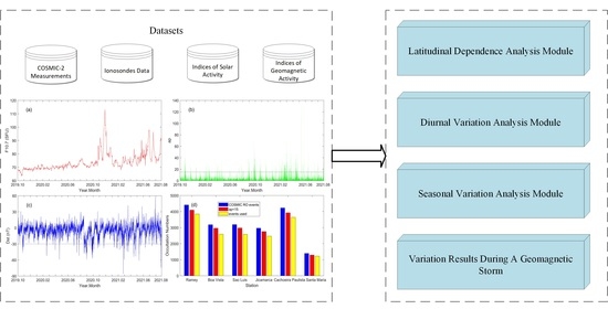
2. Datasets
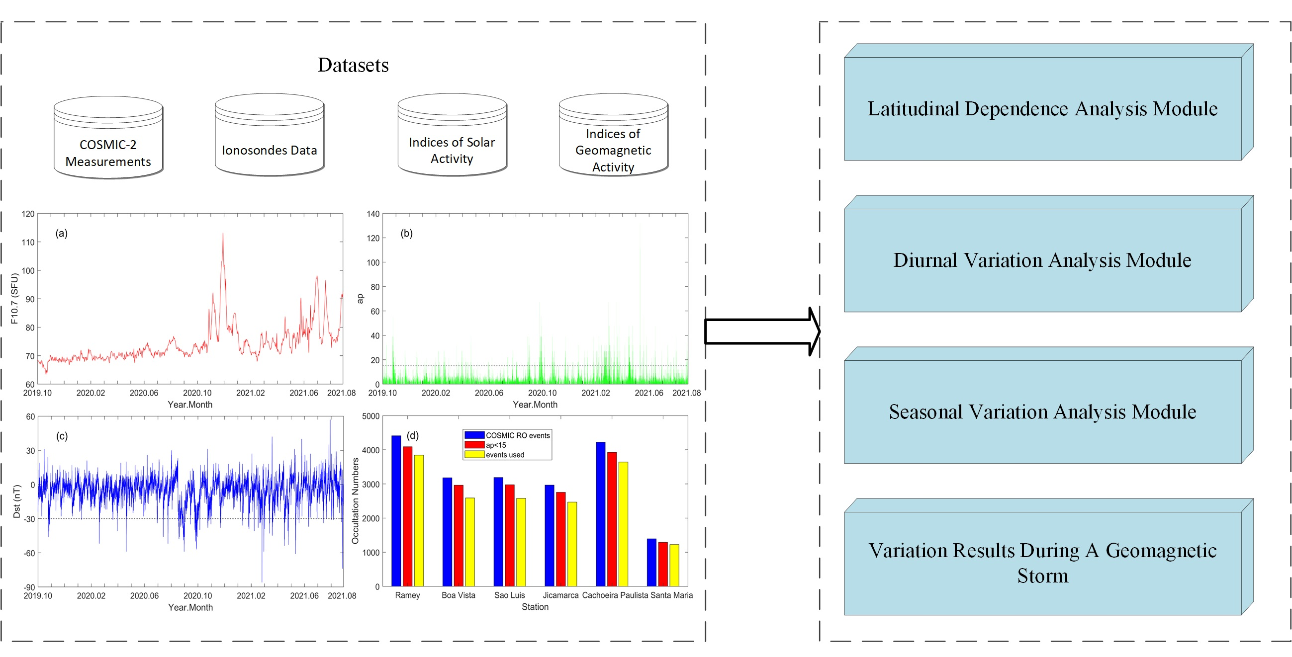
2.1. EDPs of COSMIC-2
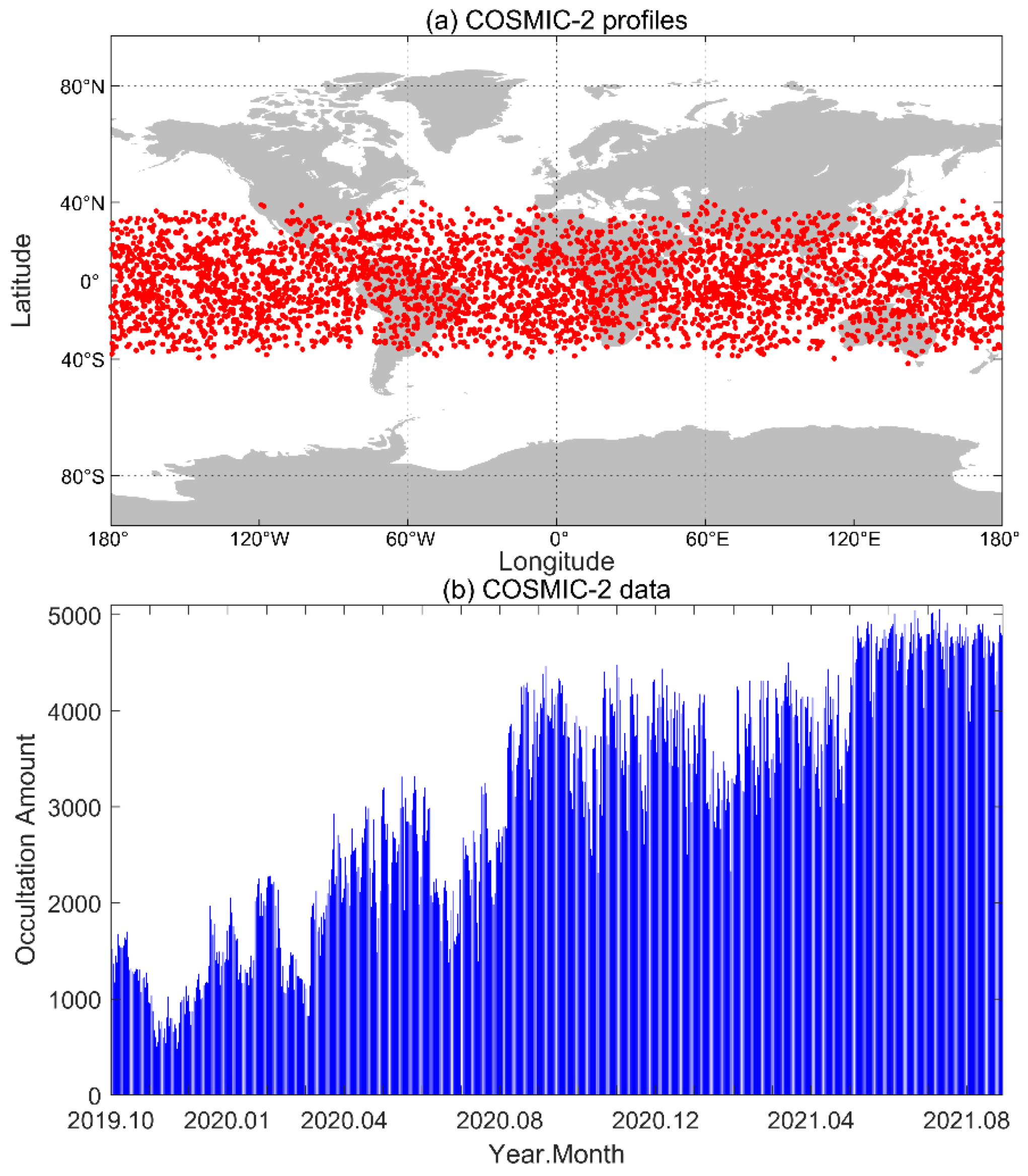
2.2. Indices of Solar Activity
2.3. Indices of Geomagnetic Activity
2.4. Ionosonde Data
3. Results
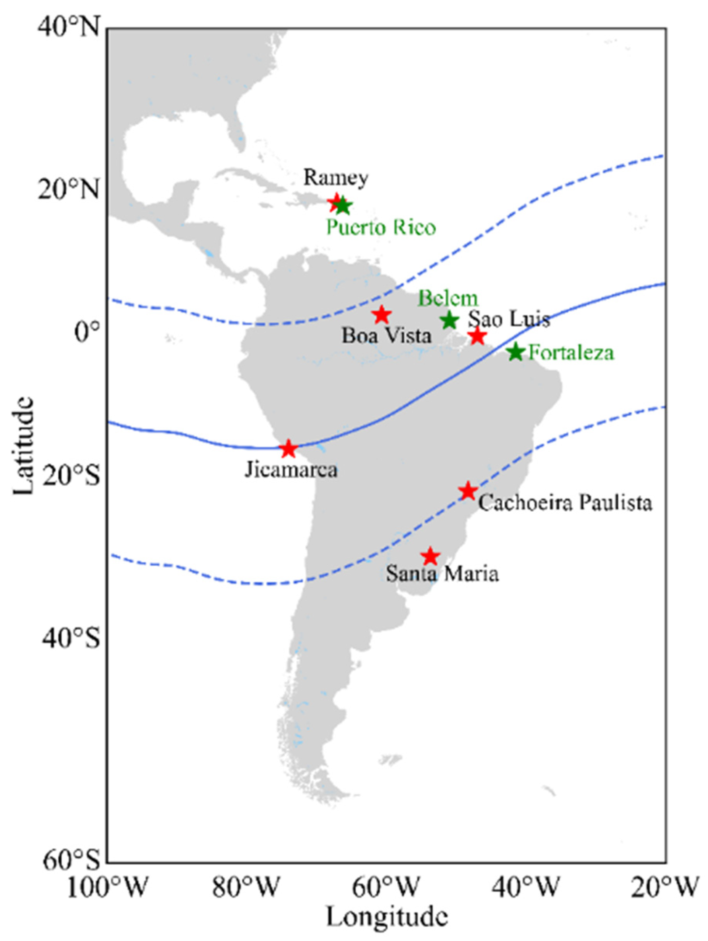
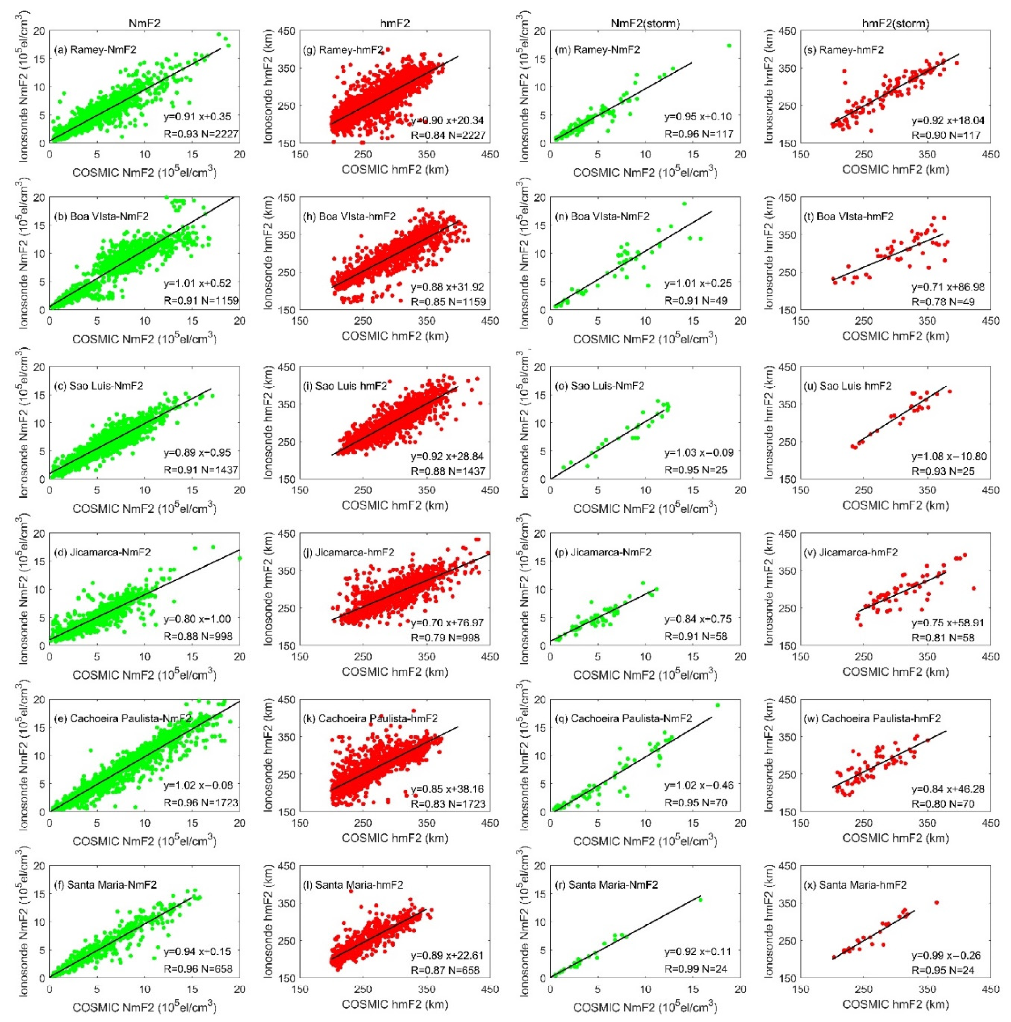
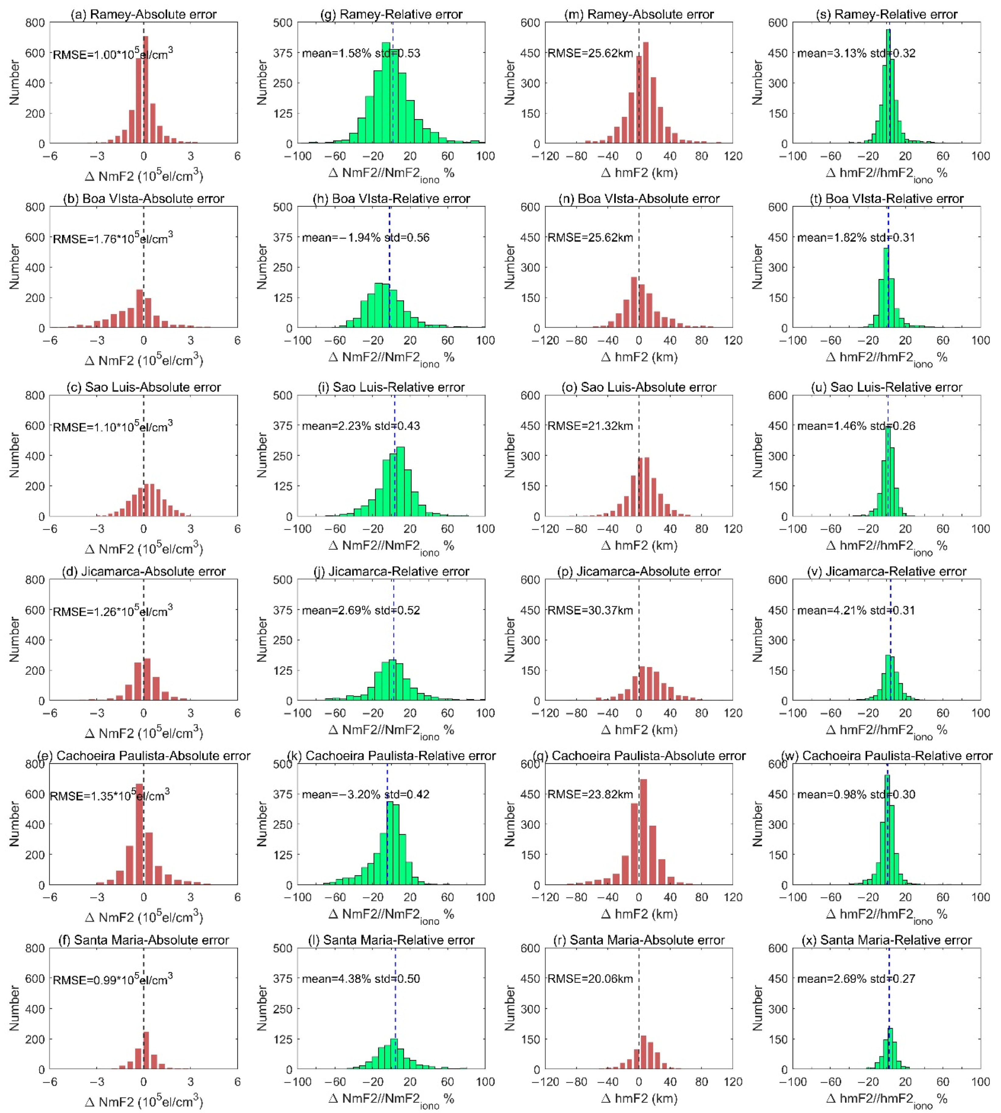
3.1. Latitudinal Dependence
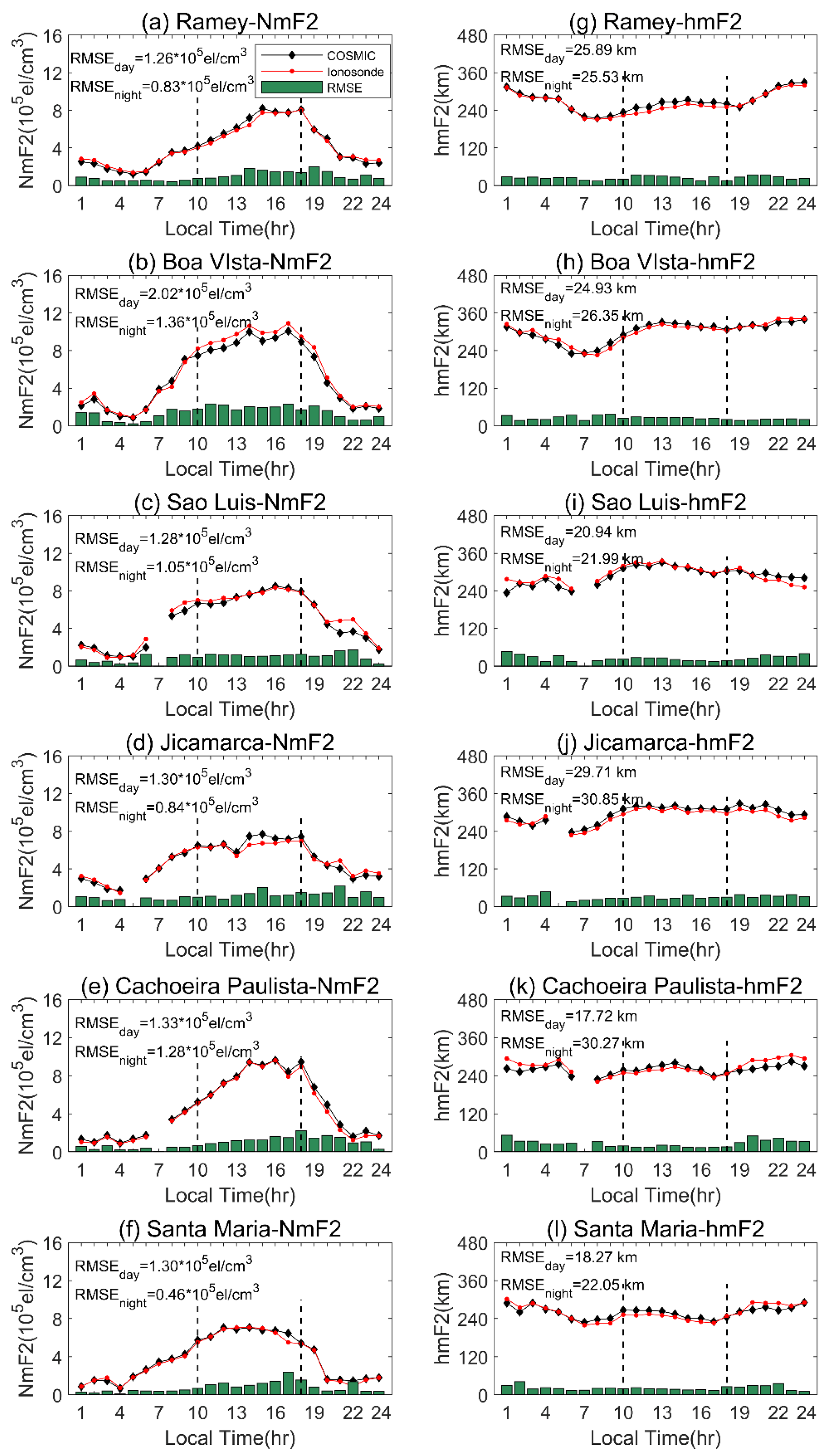
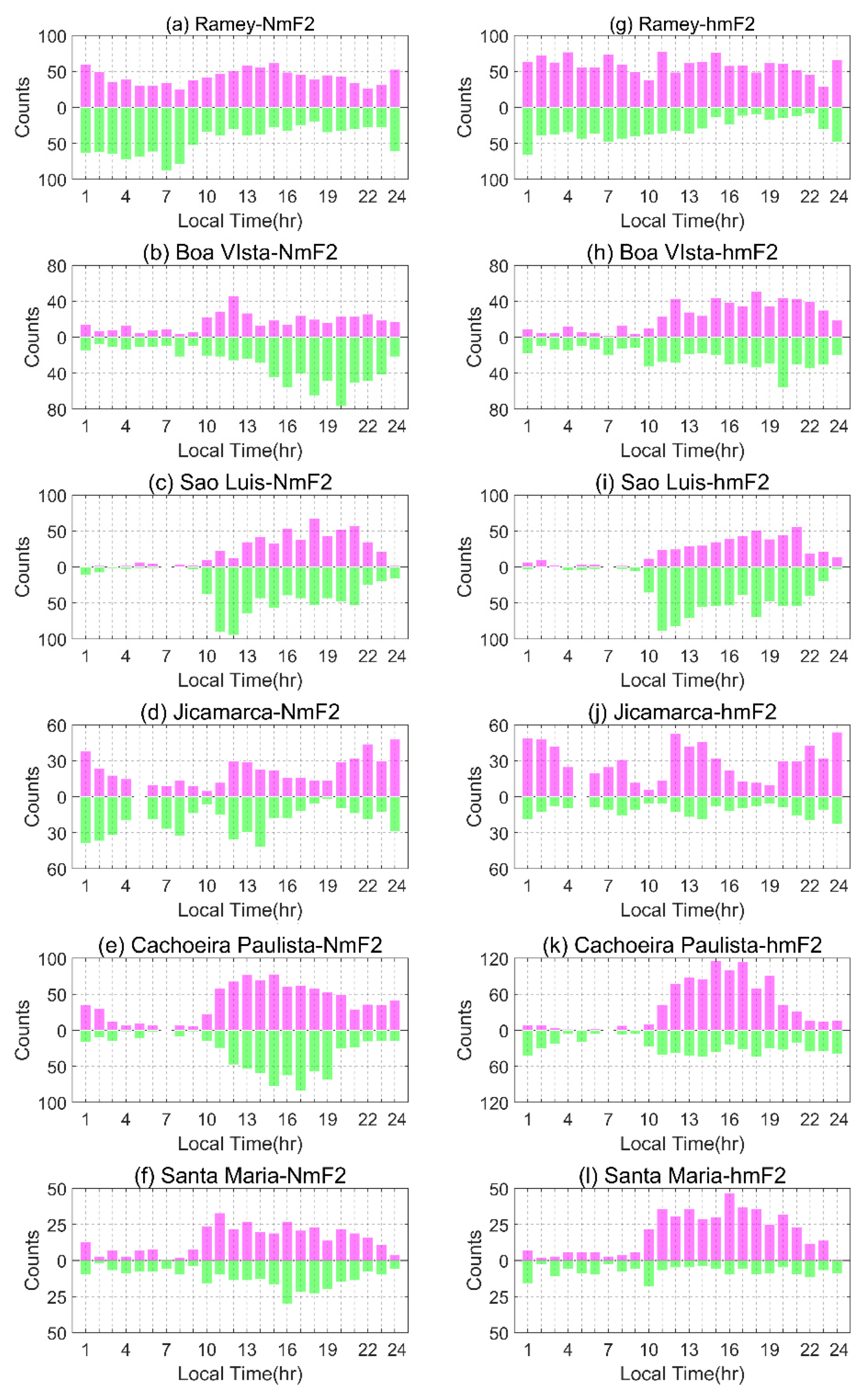
3.2. Diurnal Variation Result
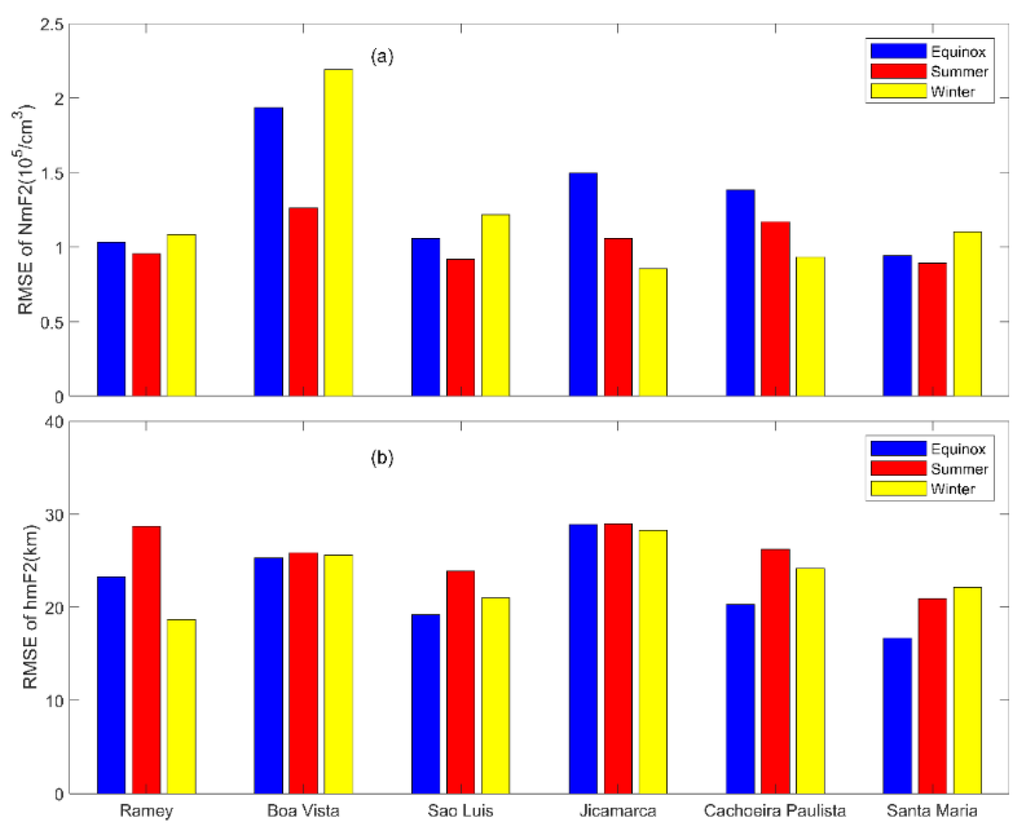
3.3. Seasonal Variation Result
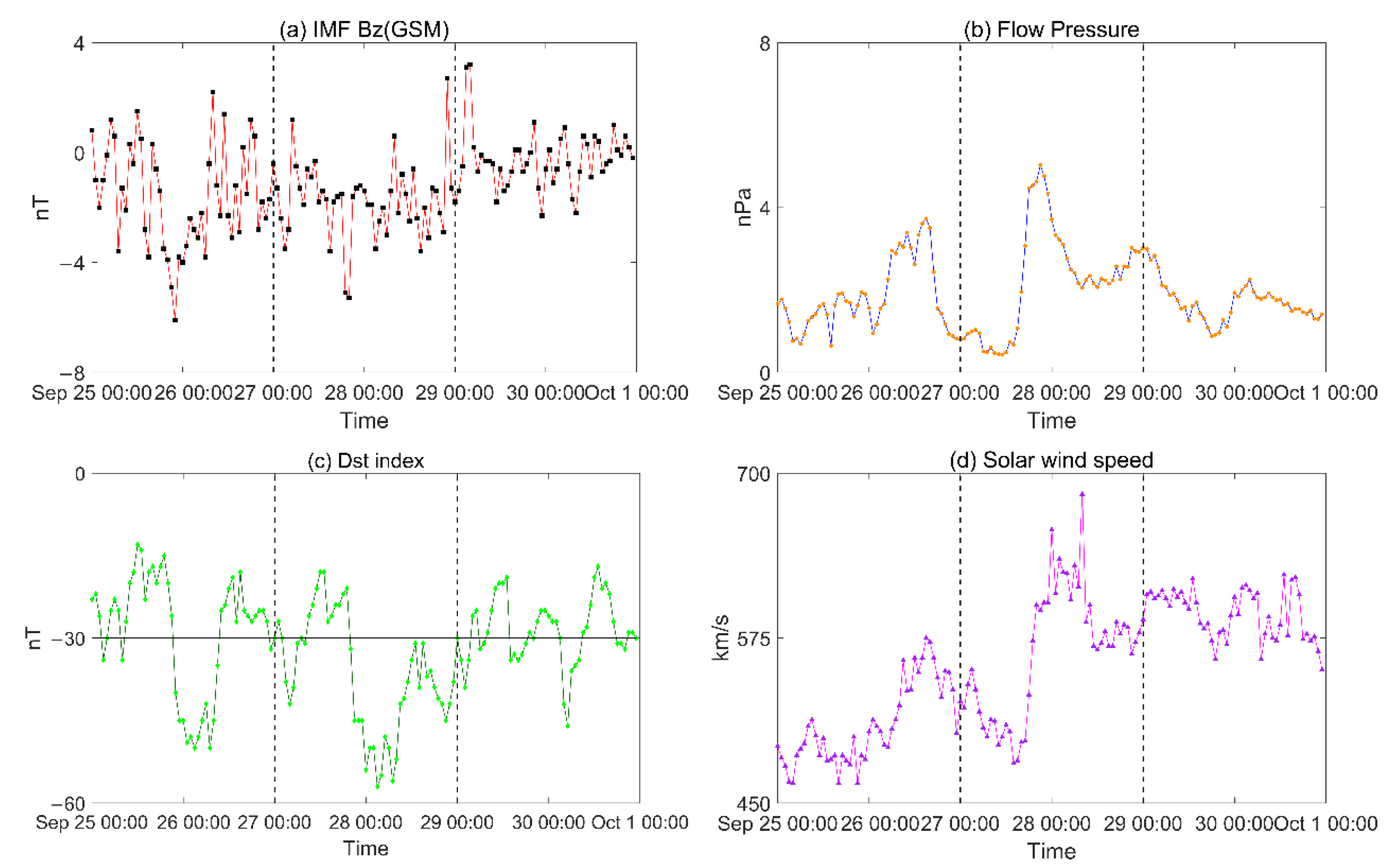
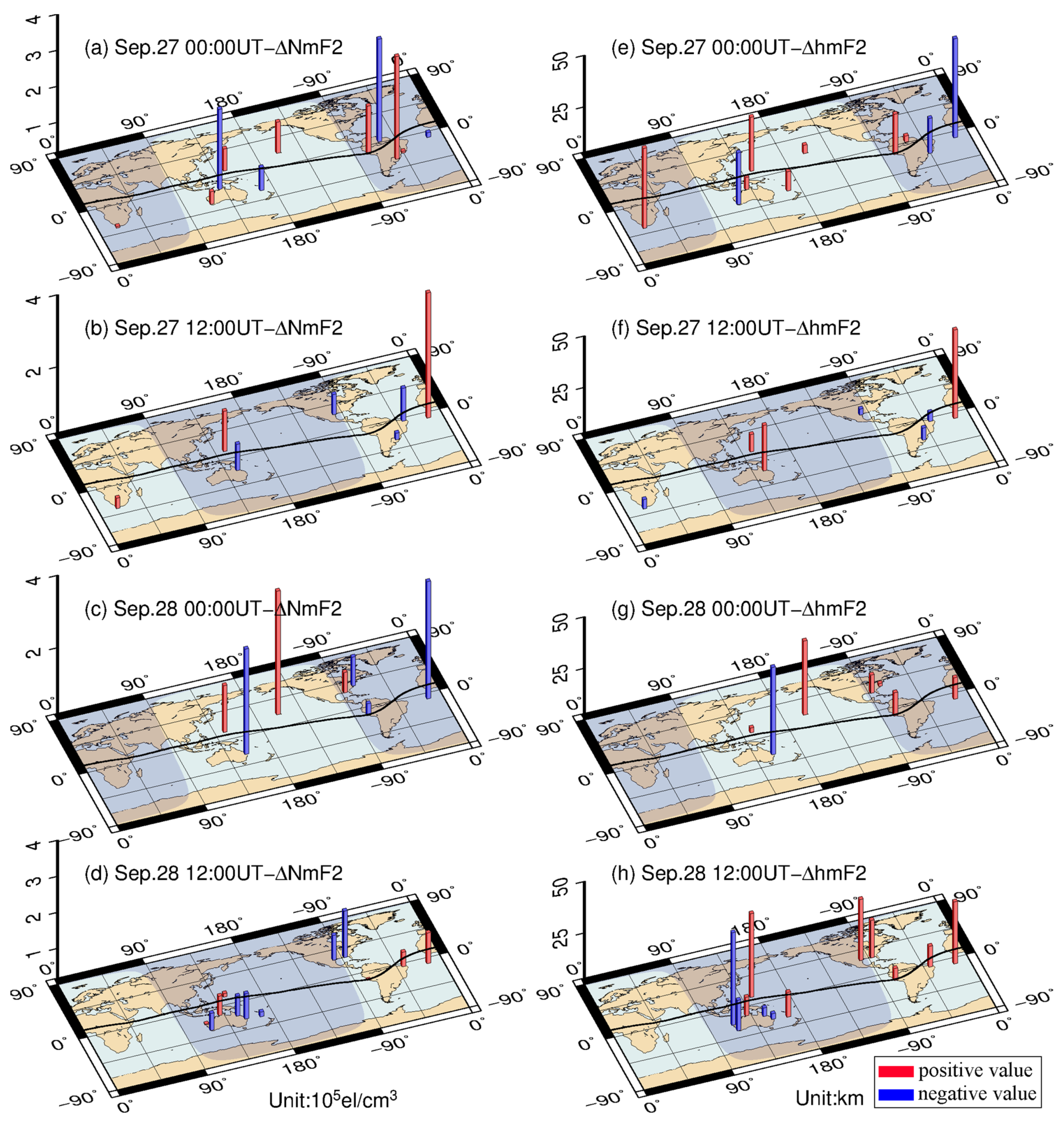
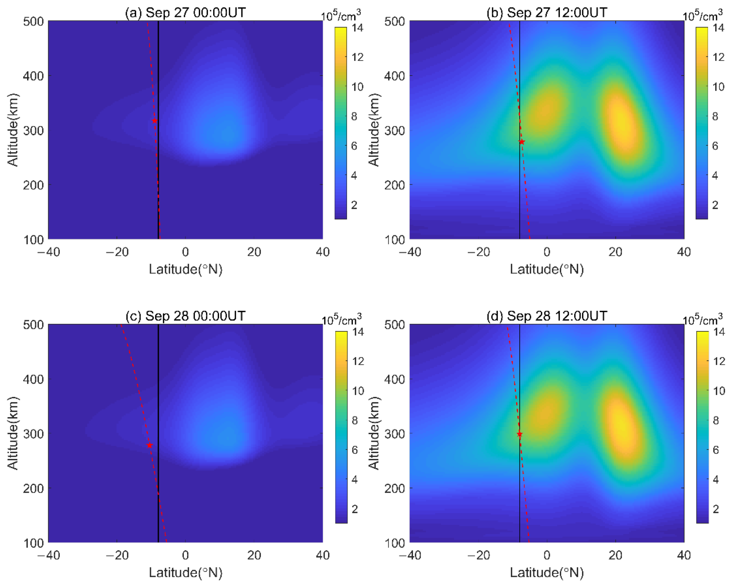
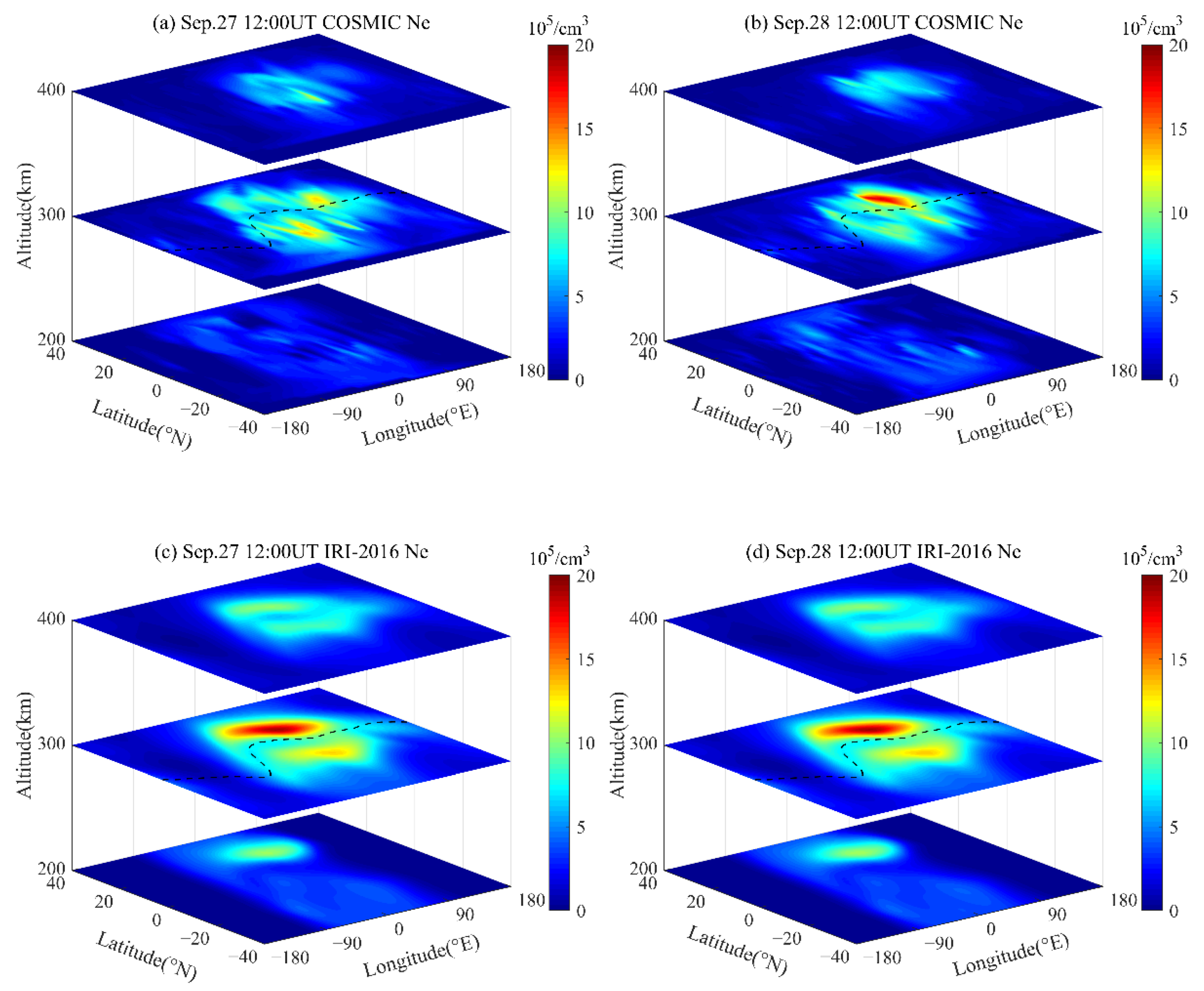
3.4. Variation Results during a Geomagnetic Storm
4. Discussion
5. Conclusions and Perspectives
Author Contributions
Funding
Institutional Review Board Statement
Informed Consent Statement
Data Availability Statement
Acknowledgments
Conflicts of Interest
Appendix A

| LT | Ramey | Boa Vista | Sao Luis | Jicamarca | Cachoeira Paulista | Santa Maria | ||||||
|---|---|---|---|---|---|---|---|---|---|---|---|---|
| RMSE | MRE | RMSE | MRE | RMSE | MRE | RMSE | MRE | RMSE | MRE | RMSE | MRE | |
| 1 | 0.90 | 20.50 | 1.39 | 29.56 | 0.66 | 29.50 | 1.07 | 23.11 | 0.60 | 61.02 | 0.28 | 18.73 |
| 2 | 0.74 | 19.85 | 1.37 | 22.24 | 0.35 | 20.41 | 0.93 | 28.04 | 0.26 | 23.21 | 0.16 | 10.08 |
| 3 | 0.52 | 18.57 | 0.43 | 19.69 | 0.52 | 55.22 | 0.64 | 24.11 | 0.65 | 47.82 | 0.39 | 17.80 |
| 4 | 0.51 | 21.30 | 0.37 | 19.05 | 0.22 | 13.93 | 0.73 | 35.94 | 0.21 | 15.01 | 0.11 | 16.18 |
| 5 | 0.48 | 20.91 | 0.23 | 22.28 | 0.34 | 30.81 | 0.25 | 16.04 | 0.44 | 21.29 | ||
| 6 | 0.61 | 26.88 | 0.48 | 26.68 | 1.25 | 37.99 | 0.92 | 29.80 | 0.42 | 29.01 | 0.39 | 18.81 |
| 7 | 0.47 | 14.93 | 1.06 | 22.28 | 0.71 | 14.34 | 0.38 | 9.91 | ||||
| 8 | 0.41 | 9.84 | 1.74 | 39.87 | 0.92 | 12.10 | 0.67 | 10.76 | 0.47 | 10.67 | 0.41 | 10.05 |
| 9 | 0.57 | 12.37 | 1.57 | 30.72 | 1.22 | 14.63 | 1.04 | 12.13 | 0.52 | 9.67 | 0.49 | 11.11 |
| 10 | 0.76 | 13.41 | 1.78 | 18.35 | 0.94 | 11.37 | 1.00 | 13.48 | 0.67 | 10.65 | 0.67 | 10.82 |
| 11 | 0.80 | 14.77 | 2.33 | 20.53 | 1.25 | 13.40 | 1.09 | 13.92 | 0.87 | 11.57 | 1.07 | 14.74 |
| 12 | 0.91 | 13.95 | 2.19 | 19.03 | 1.18 | 13.01 | 0.79 | 9.30 | 1.02 | 11.80 | 1.21 | 14.48 |
| 13 | 1.08 | 13.95 | 1.70 | 14.01 | 1.19 | 14.02 | 1.20 | 12.90 | 1.19 | 14.97 | 0.82 | 9.46 |
| 14 | 1.81 | 18.13 | 2.02 | 14.06 | 1.00 | 11.35 | 1.36 | 15.83 | 1.25 | 12.89 | 1.00 | 13.20 |
| 15 | 1.62 | 16.54 | 1.97 | 14.92 | 1.04 | 11.13 | 2.00 | 24.22 | 1.26 | 12.81 | 1.20 | 16.75 |
| 16 | 1.44 | 13.17 | 2.01 | 14.25 | 1.09 | 10.47 | 1.14 | 13.32 | 1.65 | 15.11 | 1.42 | 20.16 |
| 17 | 1.46 | 14.38 | 2.31 | 16.22 | 1.19 | 12.25 | 1.20 | 13.92 | 1.51 | 16.26 | 2.37 | 38.69 |
| 18 | 1.39 | 13.95 | 1.70 | 14.81 | 1.24 | 16.74 | 1.46 | 16.52 | 2.24 | 25.64 | 1.54 | 31.83 |
| 19 | 2.02 | 27.07 | 2.14 | 18.02 | 1.04 | 18.51 | 1.35 | 20.73 | 1.44 | 24.28 | 0.80 | 16.08 |
| 20 | 1.50 | 27.56 | 1.63 | 23.65 | 1.08 | 19.81 | 1.45 | 24.46 | 1.73 | 50.46 | 0.40 | 10.81 |
| 21 | 0.88 | 20.74 | 0.98 | 20.55 | 1.64 | 25.81 | 2.20 | 31.24 | 1.54 | 49.40 | 0.45 | 14.26 |
| 22 | 0.66 | 15.59 | 0.60 | 19.01 | 1.71 | 26.32 | 0.97 | 20.79 | 0.97 | 49.22 | 1.37 | 38.92 |
| 23 | 1.12 | 21.05 | 0.63 | 23.67 | 0.73 | 22.99 | 1.56 | 24.33 | 1.06 | 48.97 | 0.36 | 16.72 |
| 24 | 0.75 | 17.20 | 0.99 | 19.94 | 0.21 | 9.73 | 0.96 | 19.46 | 0.29 | 21.59 | 0.33 | 15.69 |
| LT | Ramey | Boa Vista | Sao Luis | Jicamarca | Cachoeira Paulista | Santa Maria | ||||||
|---|---|---|---|---|---|---|---|---|---|---|---|---|
| RMSE | MRE | RMSE | MRE | RMSE | MRE | RMSE | MRE | RMSE | MRE | RMSE | MRE | |
| 1 | 27.39 | 6.41 | 33.00 | 7.47 | 38.40 | 15.72 | 32.81 | 9.46 | 42.38 | 11.08 | 29.34 | 6.09 |
| 2 | 24.06 | 6.30 | 17.11 | 4.79 | 37.83 | 11.52 | 27.32 | 7.89 | 34.32 | 9.82 | 40.92 | 6.99 |
| 3 | 27.11 | 7.10 | 21.20 | 5.25 | 29.84 | 9.28 | 34.05 | 9.10 | 34.30 | 9.86 | 18.03 | 5.38 |
| 4 | 23.24 | 6.46 | 19.84 | 4.93 | 13.62 | 4.05 | 37.68 | 13.10 | 25.96 | 6.12 | 22.14 | 6.54 |
| 5 | 25.02 | 6.57 | 28.13 | 8.39 | 32.57 | 9.46 | 24.38 | 5.87 | 19.74 | 6.06 | ||
| 6 | 26.57 | 7.80 | 33.55 | 9.18 | 14.55 | 4.31 | 16.08 | 5.91 | 27.00 | 8.21 | 13.59 | 4.26 |
| 7 | 16.73 | 6.09 | 17.36 | 5.35 | 19.79 | 6.27 | 14.21 | 5.19 | ||||
| 8 | 13.76 | 5.32 | 35.29 | 11.78 | 17.13 | 4.68 | 21.94 | 6.18 | 32.00 | 7.57 | 19.94 | 7.34 |
| 9 | 20.21 | 7.13 | 37.89 | 11.12 | 22.54 | 5.79 | 26.38 | 7.13 | 17.24 | 5.00 | 20.56 | 7.04 |
| 10 | 19.81 | 6.85 | 24.10 | 6.61 | 22.05 | 5.30 | 27.18 | 7.83 | 19.17 | 5.35 | 18.59 | 5.85 |
| 11 | 33.07 | 11.09 | 28.38 | 7.50 | 26.76 | 6.15 | 29.75 | 8.01 | 15.68 | 4.73 | 22.43 | 7.60 |
| 12 | 32.38 | 10.08 | 26.36 | 6.70 | 25.96 | 6.01 | 33.25 | 8.22 | 15.37 | 4.77 | 18.12 | 5.62 |
| 13 | 30.09 | 9.44 | 26.71 | 6.15 | 26.01 | 5.49 | 23.41 | 6.44 | 21.26 | 7.00 | 18.01 | 6.36 |
| 14 | 27.08 | 8.32 | 26.36 | 6.00 | 21.00 | 4.94 | 26.75 | 6.81 | 19.33 | 5.55 | 16.97 | 5.49 |
| 15 | 22.65 | 6.27 | 26.67 | 6.82 | 16.47 | 4.02 | 36.58 | 9.95 | 15.09 | 4.30 | 15.05 | 4.55 |
| 16 | 14.36 | 4.27 | 22.26 | 5.31 | 17.67 | 4.66 | 27.05 | 6.29 | 13.76 | 4.52 | 16.23 | 5.80 |
| 17 | 28.10 | 7.92 | 23.96 | 5.60 | 15.10 | 4.10 | 29.49 | 6.61 | 15.64 | 4.92 | 13.60 | 4.61 |
| 18 | 15.79 | 5.19 | 19.78 | 4.87 | 17.68 | 4.31 | 29.65 | 7.71 | 15.82 | 4.76 | 25.42 | 8.10 |
| 19 | 26.63 | 6.71 | 17.40 | 4.17 | 20.41 | 4.79 | 37.93 | 8.90 | 29.57 | 6.47 | 24.03 | 7.28 |
| 20 | 33.05 | 8.43 | 18.53 | 4.70 | 24.63 | 6.96 | 29.33 | 7.45 | 50.48 | 11.83 | 29.43 | 8.00 |
| 21 | 34.17 | 8.94 | 20.59 | 4.27 | 35.98 | 10.57 | 36.98 | 9.51 | 36.71 | 9.54 | 28.20 | 7.05 |
| 22 | 28.44 | 7.07 | 20.77 | 4.42 | 31.25 | 9.39 | 32.47 | 8.95 | 43.37 | 10.29 | 35.19 | 10.09 |
| 23 | 20.61 | 4.82 | 22.53 | 4.49 | 30.23 | 9.46 | 38.02 | 10.84 | 33.84 | 8.14 | 12.92 | 4.12 |
| 24 | 22.87 | 4.85 | 20.28 | 4.78 | 39.44 | 11.66 | 31.03 | 9.42 | 33.68 | 8.86 | 10.39 | 2.82 |
| Season | Ramey | Boa Vista | Sao Luis | Jicamarca | Cachoeira Paulista | Santa Maria | ||||||
|---|---|---|---|---|---|---|---|---|---|---|---|---|
| RMSE | MRE | RMSE | MRE | RMSE | MRE | RMSE | MRE | RMSE | MRE | RMSE | MRE | |
| equinox | 1.03 | 19.99 | 1.94 | 21.74 | 1.06 | 13.80 | 1.50 | 35.18 | 1.38 | 13.99 | 0.94 | 14.20 |
| summer | 0.96 | 18.64 | 1.26 | 18.20 | 0.92 | 11.71 | 1.06 | 28.07 | 1.17 | 11.17 | 0.89 | 9.52 |
| winter | 1.09 | 22.93 | 2.19 | 24.01 | 1.22 | 22.74 | 0.85 | 22.44 | 0.93 | 10.23 | 1.10 | 18.98 |
| Season | Ramey | Boa Vista | Sao Luis | Jicamarca | Cachoeira Paulista | Santa Maria | ||||||
|---|---|---|---|---|---|---|---|---|---|---|---|---|
| RMSE | MRE | RMSE | MRE | RMSE | MRE | RMSE | MRE | RMSE | MRE | RMSE | MRE | |
| equinox | 23.30 | 6.11 | 25.29 | 5.87 | 19.22 | 4.69 | 28.90 | 7.83 | 20.30 | 5.06 | 16.71 | 5.15 |
| summer | 28.70 | 7.22 | 25.86 | 5.94 | 23.87 | 5.54 | 28.95 | 7.47 | 26.22 | 6.77 | 20.95 | 5.99 |
| winter | 18.69 | 5.57 | 25.60 | 5.74 | 21.01 | 5.43 | 28.28 | 7.22 | 24.15 | 6.21 | 22.17 | 6.38 |
| Station | Geog. Lon. (° E) | Geog. Lat. (° N) | Geom. Lat. (° N) | Sep. 27 00:00UT | Sep. 27 12:00UT | Sep. 28 00:00UT | Sep. 28 12:00UT |
|---|---|---|---|---|---|---|---|
| Ascension Island | −14.40 | −7.95 | −2.89 | x | x | x | x |
| Boa Vista | −60.70 | 2.80 | 11.98 | x | |||
| Cachoeira Paulista | −45.00 | −22.70 | −14.17 | x | |||
| Darwin | 130.95 | −12.45 | −20.96 | x | x | ||
| Guam | 144.86 | 13.62 | 6.02 | x | x | x | x |
| Hermanus | 19.22 | −34.42 | −34.03 | x | x | ||
| Jicamarca | −76.80 | −12.00 | −2.54 | x | x | x | |
| Lualualei | −158.15 | 21.43 | 21.74 | x | x | ||
| Norfolk | 167.97 | −29.03 | −33.13 | x | x | ||
| Perth | 116.13 | −32.00 | −41.11 | x | x | ||
| Santa Maria | −53.71 | −29.73 | −20.63 | x | x | ||
| Austin | −97.70 | 30.40 | 38.66 | x | x | ||
| Fortaleza | −38.40 | −3.90 | 3.91 | x | x | ||
| Townsville | 146.85 | −19.63 | −26.64 | x | x | ||
| Brisbane | 153.06 | −27.06 | −33.24 | x | x | ||
| Eglin Afb | −86.50 | 30.50 | 39.44 | x | x | ||
| Wallops Is | −75.50 | 37.90 | 47.11 | x | |||
| Learmonth | 114.10 | −21.80 | −31.01 | x |
References
- Kursinski, E.R.; Hajj, G.A.; Schofield, J.T.; Linfield, R.P.; Hardy, K.R. Observing Earth’s atmosphere with radio occultation measurements using the Global Positioning System. J. Geophys. Res. Atmos. 1997, 102, 23429–23465. [Google Scholar] [CrossRef]
- Hu, A.; Wu, S.; Wang, X.; Wang, Y.; Norman, R.; He, C.; Cai, H.; Zhang, K. Improvement of reflection detection success rate of GNSS RO measurements using artificial neural network. IEEE Trans. Geosci. Remote Sens. 2018, 56, 760–769. [Google Scholar] [CrossRef]
- Banos, I.H.; Sapucci, L.F.; Cucurull, L.; Bastarz, C.F.; Silveira, B.B. Assimilation of GPSRO bending angle profiles into the Brazilian global atmospheric model. Remote Sens. 2019, 11, 256. [Google Scholar] [CrossRef]
- Sokolovskiy, S.V.; Rocken, C.; Lenschow, D.H.; Kuo, Y.H.; Anthes, R.A.; Schreiner, W.S.; Hunt, D.C. Observing the moist troposphere with radio occultation signals from COSMIC. Geophys. Res. Lett. 2007, 34, 1–6. [Google Scholar] [CrossRef]
- Foelsche, U.; Pirscher, B.; Borsche, M.; Kirchengast, G.; Wickert, J. Assessing the climate monitoring utility of radio occultation data: From CHAMP to FORMOSAT-3/COSMIC. Terr. Atmos. Ocean. Sci. 2009, 20, 155–170. [Google Scholar] [CrossRef][Green Version]
- Tsuda, T.; Lin, X.; Hayashi, H. Analysis of vertical wave number spectrum of atmospheric gravity waves in the stratosphere using COSMIC GPS radio occultation data. Atmos. Meas. Tech. 2011, 4, 1627–1636. [Google Scholar] [CrossRef]
- Johnston, B.; Xie, F. Characterizing extratropical tropopause bimodality and its relationship to the occurrence of double tropopauses using COSMIC GPS radio occultation observations. Remote Sens. 2020, 12, 1109. [Google Scholar] [CrossRef]
- Lin, C.H.; Liu, J.Y.; Fang, T.W.; Chang, P.Y.; Tsai, H.F.; Chen, C.H.; Hsiao, C.C. Motions of the equatorial ionization anomaly crests imaged by FORMOSAT-3/COSMIC. Geophys. Res. Lett. 2007, 34, L19101. [Google Scholar] [CrossRef]
- Lin, C.H.; Wang, W.; Hagan, M.E.; Hsiao, C.C.; Immel, T.J.; Hsu, M.L.; Liu, J.Y.; Paxton, L.J.; Fang, T.W.; Liu, C.H. Plausible effect of atmospheric tides on the equatorial ionosphere observed by the FORMOSAT-3/COSMIC: Three-dimensional electron density structures. Geophys. Res. Lett. 2007, 34, 1–5. [Google Scholar] [CrossRef]
- He, M.; Liu, L.; Wan, W.; Ning, B.; Zhao, B.; Wen, J.; Yue, X.a.; Le, H. A study of the Weddell Sea Anomaly observed by FORMOSAT-3/COSMIC. J. Geophys. Res. Space Phys. 2009, 114, 1–10. [Google Scholar] [CrossRef]
- Liu, J.Y.; Lin, C.Y.; Lin, C.H.; Tsai, H.F.; Solomon, S.C.; Sun, Y.Y.; Lee, I.T.; Schreiner, W.S.; Kuo, Y.H. Artificial plasma cave in the low-latitude ionosphere results from the radio occultation inversion of the FORMOSAT-3/COSMIC. J. Geophys. Res. Space Phys. 2010, 115, 1–8. [Google Scholar] [CrossRef]
- Zakharenkova, I.E.; Krankowski, A.; Shagimuratov, I.I.; Cherniak, Y.V.; Krypiak-Gregorczyk, A.; Wielgosz, P.; Lagovsky, A.F. Observation of the ionospheric storm of October 11, 2008 using FORMOSAT-3/COSMIC data. EarthPlanets Space 2012, 64, 505–512. [Google Scholar] [CrossRef][Green Version]
- Lin, C.-H.; Liu, J.-Y.; Hsiao, C.-C.; Liu, C.-H.; Cheng, C.-Z.; Chang, P.-Y.; Tsai, H.-F.; Fang, T.-W.; Chen, C.-H.; Hsu, M.-L. Global ionospheric structure imaged by FORMOSAT-3/COSMIC: Early results. Terr. Atmos. Ocean. Sci. 2009, 20, 171–179. [Google Scholar] [CrossRef]
- Zhao, B.; Wan, W.; Yue, X.; Liu, L.; Ren, Z.; He, M.; Liu, J. Global characteristics of occurrence of an additional layer in the ionosphere observed by COSMIC/FORMOSAT-3. Geophys. Res. Lett. 2011, 38, 1–5. [Google Scholar] [CrossRef]
- Liu, J.-Y.; Lee, C.-C.; Yang, J.-Y.; Chen, C.-Y.; Reinisch, B.W. Electron density profiles in the equatorial ionosphere observed by the FORMOSAT-3/COSMIC and a digisonde at Jicamarca. GPS Solut. 2010, 14, 75–81. [Google Scholar] [CrossRef]
- Krankowski, A.; Zakharenkova, I.; Krypiak-Gregorczyk, A.; Shagimuratov, I.I.; Wielgosz, P. Ionospheric electron density observed by FORMOSAT-3/COSMIC over the European region and validated by ionosonde data. J. Geod. 2011, 85, 949–964. [Google Scholar] [CrossRef]
- Hajj, G.A.; Romans, L.J. Ionospheric electron density profiles obtained with the Global Positioning System: Results from the GPS/MET experiment. Radio Sci. 1998, 33, 175–190. [Google Scholar] [CrossRef]
- Yue, X.; Schreiner, W.S.; Lei, J.; Sokolovskiy, S.V.; Rocken, C.; Hunt, D.C.; Kuo, Y.H. Error analysis of Abel retrieved electron density profiles from radio occultation measurements. Ann. Geophys. 2010, 28, 217–222. [Google Scholar] [CrossRef]
- Tsai, L.C.; Tsai, W.H.; Schreiner, W.S.; Berkey, F.T.; Liu, J.Y. Comparisons of GPS/MET retrieved ionospheric electron density and ground based ionosonde data. EarthPlanets Space 2001, 53, 193–205. [Google Scholar] [CrossRef]
- Lei, J.; Syndergaard, S.; Burns, A.G.; Solomon, S.C.; Wang, W.; Zeng, Z.; Roble, R.G.; Wu, Q.; Kuo, Y.-H.; Holt, J.M.; et al. Comparison of COSMIC ionospheric measurements with ground-based observations and model predictions: Preliminary results. J. Geophys. Res. Space Phys. 2007, 112, 1–10. [Google Scholar] [CrossRef]
- Yang, K.-F.; Chu, Y.-H.; Su, C.-L.; Ko, H.-T.; Wang, C.-Y. An examination of FORMOSAT-3/COSMIC ionospheric electron density profile: Data quality criteria and comparisons with the IRI model. Terr. Atmos. Ocean. Sci. 2009, 20, 193–206. [Google Scholar] [CrossRef]
- Ely, C.V.; Batista, I.S.; Abdu, M.A. Radio occultation electron density profiles from the FORMOSAT-3/COSMIC satellites over the Brazilian region: A comparison with Digisonde data. Adv. Space Res. 2012, 49, 1553–1562. [Google Scholar] [CrossRef]
- Cherniak, I.V.; Zakharenkova, I.E. Validation of FORMOSAT-3/COSMIC radio occultation electron density profiles by incoherent scatter radar data. Adv. Space Res. 2014, 53, 1304–1312. [Google Scholar] [CrossRef]
- Hu, L.; Ning, B.; Liu, L.; Zhao, B.; Chen, Y.; Li, G. Comparison between ionospheric peak parameters retrieved from COSMIC measurement and ionosonde observation over Sanya. Adv. Space Res. 2014, 54, 929–938. [Google Scholar] [CrossRef]
- Hu, L.; Ning, B.; Liu, L.; Zhao, B.; Li, G.; Wu, B.; Huang, Z.; Hao, X.; Chang, S.; Wu, Z. Validation of COSMIC ionospheric peak parameters by the measurements of an ionosonde chain in China. Ann. Geophys. 2014, 32, 1311–1319. [Google Scholar] [CrossRef]
- McNamara, L.F.; Thompson, D.C. Validation of COSMIC values of foF2 and M(3000)F2 using ground-based ionosondes. Adv. Space Res. 2015, 55, 163–169. [Google Scholar] [CrossRef]
- Luo, J.; Sun, F.; Xu, X.; Wang, H. Ionospheric F2-Layer critical frequency retrieved from COSMIC radio occultation: A statistical comparison with measurements from a meridional ionosonde chain over Southeast Asia. Adv. Space Res. 2019, 63, 327–336. [Google Scholar] [CrossRef]
- Bilitza, D.; Altadill, D.; Truhlik, V.; Shubin, V.; Galkin, I.; Reinisch, B.; Huang, X. International Reference Ionosphere 2016: From ionospheric climate to real-time weather predictions. Space Weather 2017, 15, 418–429. [Google Scholar] [CrossRef]
- Bilitza, D. IRI the International Standard for the Ionosphere. Adv. Radio Sci. 2018, 16, 1–11. [Google Scholar] [CrossRef]
- Lin, C.Y.; Lin, C.C.H.; Liu, J.Y.; Rajesh, P.K.; Matsuo, T.; Chou, M.Y.; Tsai, H.F.; Yeh, W.H. The early results and validation of FORMOSAT-7/COSMIC-2 space weather products: Global ionospheric specification and Ne-Aided Abel electron density profile. J. Geophys. Res. Space Phys. 2020, 125, e2020JA028028. [Google Scholar] [CrossRef]
- Cherniak, I.; Zakharenkova, I.; Braun, J.; Wu, Q.; Pedatella, N.; Schreiner, W.; Weiss, J.-P.; Hunt, D. Accuracy assessment of the quiet-time ionospheric F2 peak parameters as derived from COSMIC-2 multi-GNSS radio occultation measurements. J. Space Weather Space Clim. 2021, 11, 18. [Google Scholar] [CrossRef]
- Okoh, D.; Seemala, G.; Rabiu, B.; Habarulema, J.B.; Jin, S.; Shiokawa, K.; Otsuka, Y.; Aggarwal, M.; Uwamahoro, J.; Mungufeni, P.; et al. A neural network-based ionospheric model over Africa from Constellation Observing System for Meteorology, Ionosphere, and Climate and ground Global Positioning System observations. J. Geophys. Res. Space Phys. 2019, 124, 10512–10532. [Google Scholar] [CrossRef]
- Li, W.; Zhao, D.; He, C.; Hu, A.; Zhang, K. Advanced machine learning optimized by the genetic algorithm in ionospheric models using long-term multi-instrument observations. Remote Sens. 2020, 12, 866. [Google Scholar] [CrossRef]
- Cander, L.R.; Mihajlovic, S.J. Forecasting ionospheric structure during the great geomagnetic storms. J. Geophys. Res. Space Phys. 1998, 103, 391–398. [Google Scholar] [CrossRef]
- Kumar, S.; Singh, R.P.; Tan, E.L.; Singh, A.K.; Ghodpage, R.N.; Siingh, D. Temporal and spatial deviation in F2 peak parameters derived from FORMOSAT-3/COSMIC. Space Weather 2016, 14, 391–405. [Google Scholar] [CrossRef]
- Schreiner, W.S.; Sokolovskiy, S.V.; Rocken, C.; Hunt, D.C. Analysis and validation of GPS/MET radio occultation data in the ionosphere. Radio Sci. 1999, 34, 949–966. [Google Scholar] [CrossRef]
- Reinisch, B.W.; Huang, X. Automatic calculation of electron density profiles from digital ionograms: 3. Processing of bottomside ionograms. Radio Sci. 1983, 18, 477–492. [Google Scholar] [CrossRef]
- Galkin, I.A.; Khmyrov, G.M.; Kozlov, A.V.; Reinisch, B.W.; Huang, X.; Paznukhov, V.V. The ARTIST 5. AIP Conf. Proc. 2008, 974, 150–159. [Google Scholar] [CrossRef]
- Reinisch, B.W.; Galkin, I.A. Global Ionospheric Radio Observatory (GIRO). EarthPlanets Space 2011, 63, 377–381. [Google Scholar] [CrossRef]
- Chu, Y.-H.; Su, C.-L.; Ko, H.-T. A global survey of COSMIC ionospheric peak electron density and its height: A comparison with ground-based ionosonde measurements. Adv. Space Res. 2010, 46, 431–439. [Google Scholar] [CrossRef]
- Chuo, Y.J.; Lee, C.C.; Chen, W.S.; Reinisch, B.W. Comparison of the characteristics of ionospheric parameters obtained from FORMOSAT-3 and digisonde over Ascension Island. Ann. Geophys. 2013, 31, 787–794. [Google Scholar] [CrossRef]
- Tsurutani, B.T.; Verkhoglyadova, O.P.; Mannucci, A.J.; Saito, A.; Araki, T.; Yumoto, K.; Tsuda, T.; Abdu, M.A.; Sobral, J.H.A.; Gonzalez, W.D.; et al. Prompt penetration electric fields (PPEFs) and their ionospheric effects during the great magnetic storm of 30–31 October 2003. J. Geophys. Res. Space Phys. 2008, 113, 1–10. [Google Scholar] [CrossRef]
- Boudouridis, A.; Zesta, E.; Lyons, L.R.; Anderson, P.C.; Lummerzheim, D. Enhanced solar wind geoeffectiveness after a sudden increase in dynamic pressure during southward IMF orientation. J. Geophys. Res. 2005, 110, 1–15. [Google Scholar] [CrossRef]
- Adebesin, B.O.; Ikubanni, S.O.; Kayode, J.S. Solar wind dynamic pressure depency on the plasma flow speed and IMF Bz during different geomagnetic activities. World J. Young Res. 2012, 2, 43–54. [Google Scholar]
- Wu, X.; Hu, X.; Gong, X.; Zhang, X.; Wang, X. Analysis of inversion errors of ionospheric radio occultation. GPS Solut. 2009, 13, 231–239. [Google Scholar] [CrossRef]
- Kumar, S.; Tan, E.L.; Razul, S.G.; See, C.M.S.; Siingh, D. Validation of the IRI-2012 model with GPS-based ground observation over a low-latitude Singapore station. EarthPlanets Space 2014, 66, 1–17. [Google Scholar] [CrossRef]
- Timoçin, E.; Ünal, İ.; Göker, Ü.D. A comparison of IRI-2016 foF2 predictions with the observations at different latitudes during geomagnetic storms. Geomagn. Aeron. 2019, 58, 846–856. [Google Scholar] [CrossRef]
- Endeshaw, L. Testing and validating IRI-2016 model over Ethiopian ionosphere. Astrophys. Space Sci. 2020, 365, 1–13. [Google Scholar] [CrossRef]


| Station | Geographic Longitude (° E) | Geographic Latitude (° N) | Geomagnetic Latitude (° N) |
|---|---|---|---|
| Ramey | −67.10 | 18.50 | 27.75 |
| Boa Vista | −60.70 | 2.80 | 11.98 |
| Sao Luis | −44.20 | −2.60 | 5.69 |
| Jicamarca | −76.80 | −12.00 | −2.54 |
| Cachoeira Paulista | −45.00 | −22.70 | −14.17 |
| Santa Maria | −53.71 | −29.73 | −20.63 |
| Station | NmF2 | hmF2 | ||||||
|---|---|---|---|---|---|---|---|---|
| R | RMSE (105 el/cm3) | MAE (105 el/cm3) | Mean|RelE| (%) | R | RMSE (km) | MAE (km) | Mean|RelE| (%) | |
| Ramey | 0.93 | 1.00 | 0.62 | 17.86 | 0.84 | 25.62 | 17.80 | 7.06 |
| Boa Vista | 0.91 | 1.76 | 1.25 | 20.01 | 0.85 | 25.62 | 18.11 | 6.46 |
| Sao Luis | 0.91 | 1.10 | 0.86 | 18.99 | 0.88 | 21.32 | 15.90 | 5.25 |
| Jicamarca | 0.88 | 1.26 | 0.82 | 19.26 | 0.79 | 30.37 | 22.60 | 7.95 |
| Cachoeira Paulista | 0.96 | 1.35 | 0.90 | 19.64 | 0.83 | 23.82 | 15.81 | 6.08 |
| Santa Maria | 0.96 | 0.99 | 0.61 | 16.00 | 0.87 | 20.06 | 14.90 | 5.99 |
Publisher’s Note: MDPI stays neutral with regard to jurisdictional claims in published maps and institutional affiliations. |
© 2021 by the authors. Licensee MDPI, Basel, Switzerland. This article is an open access article distributed under the terms and conditions of the Creative Commons Attribution (CC BY) license (https://creativecommons.org/licenses/by/4.0/).
Share and Cite
Shi, S.; Li, W.; Zhang, K.; Wu, S.; Shi, J.; Song, F.; Sun, P. Validation of COSMIC-2-Derived Ionospheric Peak Parameters Using Measurements of Ionosondes. Remote Sens. 2021, 13, 4238. https://doi.org/10.3390/rs13214238
Shi S, Li W, Zhang K, Wu S, Shi J, Song F, Sun P. Validation of COSMIC-2-Derived Ionospheric Peak Parameters Using Measurements of Ionosondes. Remote Sensing. 2021; 13(21):4238. https://doi.org/10.3390/rs13214238
Chicago/Turabian StyleShi, Shuangshuang, Wang Li, Kefei Zhang, Suqin Wu, Jiaqi Shi, Fucheng Song, and Peng Sun. 2021. "Validation of COSMIC-2-Derived Ionospheric Peak Parameters Using Measurements of Ionosondes" Remote Sensing 13, no. 21: 4238. https://doi.org/10.3390/rs13214238
APA StyleShi, S., Li, W., Zhang, K., Wu, S., Shi, J., Song, F., & Sun, P. (2021). Validation of COSMIC-2-Derived Ionospheric Peak Parameters Using Measurements of Ionosondes. Remote Sensing, 13(21), 4238. https://doi.org/10.3390/rs13214238