Abstract
Agricultural greenhouses (AGs) are an important component of modern facility agriculture, and accurately mapping and dynamically monitoring their distribution are necessary for agricultural scientific management and planning. Semantic segmentation can be adopted for AG extraction from remote sensing images. However, the feature maps obtained by traditional deep convolutional neural network (DCNN)-based segmentation algorithms blur spatial details and insufficient attention is usually paid to contextual representation. Meanwhile, the maintenance of the original morphological characteristics, especially the boundaries, is still a challenge for precise identification of AGs. To alleviate these problems, this paper proposes a novel network called high-resolution boundary refined network (HBRNet). In this method, we design a new backbone with multiple paths based on HRNetV2 aiming to preserve high spatial resolution and improve feature extraction capability, in which the Pyramid Cross Channel Attention (PCCA) module is embedded to residual blocks to strengthen the interaction of multiscale information. Moreover, the Spatial Enhancement (SE) module is employed to integrate the contextual information of different scales. In addition, we introduce the Spatial Gradient Variation (SGV) unit in the Boundary Refined (BR) module to couple the segmentation task and boundary learning task, so that they can share latent high-level semantics and interact with each other, and combine this with the joint loss to refine the boundary. In our study, GaoFen-2 remote sensing images in Shouguang City, Shandong Province, China are selected to make the AG dataset. The experimental results show that HBRNet demonstrates a significant improvement in segmentation performance up to an IoU score of 94.89%, implying that this approach has advantages and potential for precise identification of AGs.
1. Introduction
Agricultural greenhouses (AGs) are a common cultivation facility of modern installation agriculture and are also an important managing object for facility agriculture. With the advantage of reducing the impacts of the external environment, such as adverse climate conditions, AGs could extend the growing season and increase crop yield significantly [1,2,3,4], and are considered an evolutionary transition from extensive to intensive farming [5].
Since the first generation of AGs was used in 1950s [6], the total coverage of AGs has reached 3.019 million hectares globally [7], mostly distributed in North Africa, the Middle East, Europe (Mediterranean areas) and China [1,8,9]. According to statistical reports released by officials in 2017, the cover area of AGs in China is up to 0.981 million hectares and the proportion has been ranked first worldwide for a long time [10]. However, since most materials used are difficult to be completely degraded by the natural environment [11,12], AGs raise wide concerns and criticism from many for posing environmental issues caused by rapid expansion, such as soil pollution, plastic waste, biological degradation and farmland destruction [13,14]. As a result, it is necessary to map and estimate AG coverage accurately and effectively, as it is significant to the sustainable development of regional agriculture and environmental conservation [15].
Remote sensing images (RSIs) from satellites and aerial platforms are widely used in various fields, such as land-use mapping [16], disaster monitoring [17] or urban planning [18,19]. AG mapping using high resolution imagery has attracted increased attention. However, features of RSIs obtained by sensors vary greatly under different atmospheric conditions or solar illuminance. Moreover, construction materials vary in transmittance and reflectivity, and together with pixel confusion caused by semitransparent film and plant crops present a highly dispersed and heterogeneous appearance and bring challenges to the identification of AGs [20].
Traditional manual acquisition methods, such as visual interpretation implemented according to image characteristics by interpretation experts, are time-consuming and laborious [21]. The accuracy is decided by expertise and experience, which cannot meet the demand of automated large-scale extraction. Recently, many approaches for AG extraction by using RSIs have been proposed, which can be divided into pixel-based and object-oriented classification methods in terms of the types of basic units. The pixel-based (PB) method [22,23,24] is performed on a single pixel and considers only spectral characteristics of different wavebands, which can cause “salt and pepper noise” [25] and deterioration in accuracy. Unlike the PB approach, the object-oriented method [26,27] focuses on units composed of several homogeneous and adjacent pixels [28]. This method can not only make use of the spectral information but also takes into account the texture, shape and structure of greenhouse patches, which effectively avoids noise and minimizes confusion of similar types [29]. Nevertheless, because of the requirement to manually design and filter features, that is, to analyze their relationship and select an optimal combination of features, there are still shortcomings of insufficient intelligence and unreasonable segmentation, such as under-segmentation and over-segmentation.
In recent years, deep learning technology [30,31], particularly deep convolutional neural networks (DCNN), has been applied to various fields such as semantic segmentation and object detection. DCNN can automatically and effectively extract hierarchical features from initial input, which surpasses traditional methods in many visual tasks [32]. Since the fully convolutional network (FCN) [33] was first proposed, semantic segmentation [34,35,36,37,38], a pixel-level classification task which aims to assign each pixel to a componential category [39], has been developed rapidly. On the basis of FCN, some state-of-the-art (SOTA) semantic segmentation frameworks have been proposed, such as UNet [40], SegNet [41], PSPNet [42] and DeepLab series [43,44,45,46], remarkably improving the performance of segmentation. In the latest research, HRNetV1 [47] and HRNetV2 [48] were proposed successively to address multiscale feature extraction through high-resolution DCNN and reached a new achievement in semantic segmentation. Drawing inspiration from human vision, the attention mechanism [49] was gradually applied to DCNN, especially in natural language processing and computer vision [50], which has become a popular strategy for increasing the accuracy of semantic segmentation networks. Some particular modules have been designed, such as the squeeze and excitation network [51], which focus on the independence between channels. A nonlocal neural network [52] was put forward to capture the long-distance spatial dependence between pixels, thus enhancing the expression by gathering specific global information for each pixel. Some of the latest research includes GCNet [53], CBAM [54] and DANet [55], which combine attention blocks of both spatial and channel dimensions.
Enlightened by the great success of DCNN in natural images [56,57,58], researchers have extended it to remote sensing image processing in diverse applications, such as land use land cover (LULC) [59], which shows that AGs extraction from RSIs can also highly benefit from semantic segmentation. For example, Yang et al. [60] compared the performance of SegNet and FCN in identifying plastic agricultural mulches on UAV aerial images. Baghirli et al. [61] employed two modified variations based on UNet architecture incorporating dilated convolutions and skip connections to identify AGs on images obtained by SPOT-7. Sun et al. [62] utilized two-temporal Sentinel-2 imageries acquired in different seasons and a one-dimensional DCNN for mapping.
In previous research, encoder–decoder frameworks [40,41] have mainly been adopted in DCNN-based AG identification algorithms. Although the resolution of an image is gradually rebuilt by fusing shallow features at the decoder stage, these methods still lose details of the spatial information through down-sampling operations, such as precise localized edges and geometric shapes. Specifically, since low-level coarse features could introduce noise, incorrect identification often occurs; for example, some buildings and factories with similar characteristics are misclassified as AGs. In addition, although some attempts have been made to solve multiscale problems [63,64,65], the local receptive fields (RFs) still limit the feature expression to a certain extent, leading to insufficient context aggregation information, thereby small AGs may be ignored, and some large-scale measures are discontinuous and holey. Moreover, multispan greenhouses (the overall AGs with large area integrated by original independent single-room greenhouses through reasonable design and excellent materials) are distributed in dense blocks, while most independent greenhouses are scattered and fragmented. How to maintain original morphological features, such as right angles and straight lines, is still a challenge to face. Some studies [66,67] have made efforts to obtain boundary information or utilize extra processing to improve the results of segmentation, yet the tedious operations, such as separate two-stream architecture or two subnets, cost more time.
To address the problems mentioned above, in this study a novel framework called high-resolution boundary refined network (HBRNet) is proposed on the basis of HRNetV2 aiming to extract AGs from RSIs more accurately, especially for boundary regions. First, we proposed the Pyramid Cross Channel Attention (PCCA) module and combined it with the basic residual module of ResNet [68] to generate two new residual units, which serve as basic elements of new backbone characterized by more powerful feature extraction capability. Then, the Spatial Enhancement (SE) module is introduced to aggregate multiscale information, eliminating problems arising from AGs of various sizes, namely scale inconsistency. Finally, the Boundary Refined (BR) module is designed to pay close attention to the edge pixels, correspondingly, the joint loss function derived from segmentation loss (SegLoss) and boundary constraint loss (BCLoss) is designed to supervise the learning procedure.
The main three contributions in this study are summarized as follows:
- We develop a parallel resolution-preserved convolutional network named HBRNet to accurately and effectively extract multiscale AGs. Unlike HRNetV2 and other approaches, two new residual blocks embedded with the PCCA module are employed to form a new backbone, realizing the interaction of cross-channel information.
- Based on the parallel multibranch architecture, we develop the SE module to capture more dense multiscale contextual information. This module is a combination of the Dense Cascaded Atrous Spatial Pyramid Pooling (DCASPP), a global encoding module and a skip connection, improving the segmentation accuracy of categories at different scales.
- We propose the BR module and the joint loss composed of SegLoss and BCLoss. Under the restriction, the edge morphology maintenance is significantly improved. Specifically, the Spatial Gradient Variation (SGV) unit and the joint loss both combine the segmentation task and the boundary task so that they can interact with each other, facilitating the convergence of the framework.
2. Study Area and Dataset
The study area is briefly introduced in Section 2.1 and Section 2.2 describes the data sources and the process of data preprocessing in detail.
2.1. Study Area
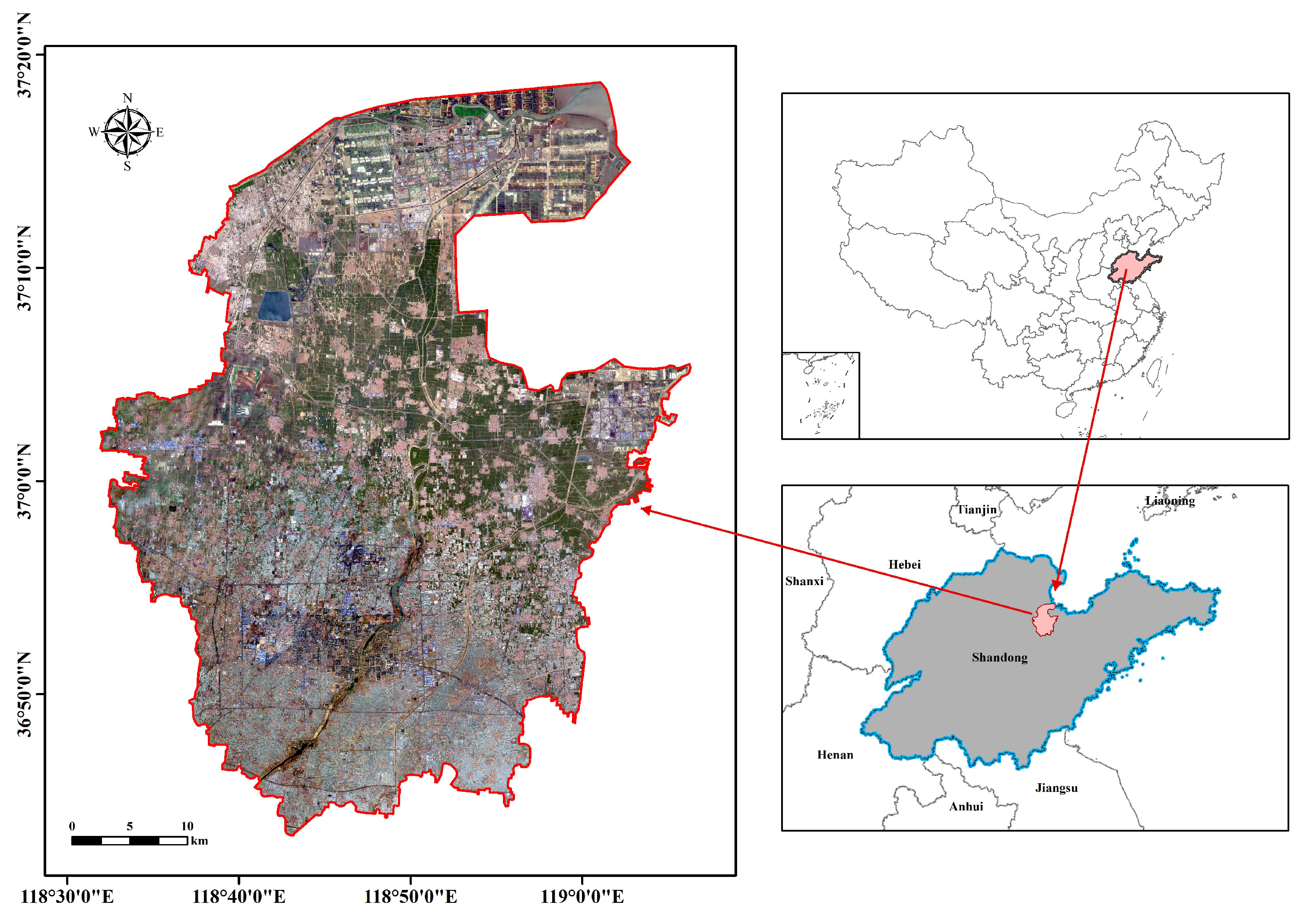
The study area is Shouguang City (36°41′~37°19′N, 118°32′~119°10′E), which is located in the northwest of Weifang, Shandong Province, China (Figure 1). It is an agricultural region adjoining cities of Hanting, Changle, Qingzhou and GuangRao, covering 2072 square kilometers in total. This area is located in a temperate zone with a continental monsoon climate characterized by four distinct seasons, where the hot rainy summer is particularly favorable for crop growth. Therefore, AGs have expanded rapidly in the past few decades and gradually have become the largest vegetable production base in China, so that the city is known as “China’s Vegetable Township” [69]. According to our field survey, the most widely used materials for AGs are transparent and translucent plastics and March to May is the high production period of crops by AGs [15].

Figure 1.
The location of the study area. Coordinate system: WGS_1984_UTM_Zone_50N.
2.2. Dataset and Preprocessing
In this study, GaoFen-2 (GF-2) images were collected to create the experimental dataset. Since the platform is equipped with two high-resolution scanners, the GF-2 images contain four multispectral bands with a spatial resolution of 3.2 m and a panchromatic band with 0.8 m. Table 1 introduces the payload parameters of the GF-2 satellite [70].

Table 1.
Payload parameters of GF-2 satellite.
To take full advantage of all spectral information, geometric orthorectification was conducted using Rational Polynomial Coefficient polynomial [71], then the pansharpening method [72] was adopted to fuse multispectral and panchromatic bands, obtaining a 0.8 m resolution image with four wavebands including blue (B), green (G), red (R) and near infrared (NIR); the bit depth is unified to 8 bits. All the above preprocessing processes were implemented based on PCI Geo Imaging Accelerator software. The ground-truth binary maps, denoting AGs and background, were manually labeled via visual interpretation with Photoshop CC 2017. In our experiment, 20 images for regions of interest were selected for the dataset, which were acquired at different times and evenly distributed over the study region to guarantee the diversity and adequacy of samples. The size of each image ranged from 1604 × 1465 pixels to 6477 × 7557 pixels. Due to their large size, we randomly clipped them to patches of 512 × 512 pixels. To fit in with the GPU’s capacity, all patches were randomly divided into training and test sets at a ratio of 8:2 and all four wavelengths were employed to evaluate the performance of our method. Note that a small part of the training samples was used for validation. Finally, 6700 tiles of images were generated totally, with 4020, 670 and 2010 tiles in the training, validation and test sets, respectively.
3. Methodology
In this section, we introduce the proposed method in detail. An overview of the network structure is first briefly presented in Section 3.1. Then Section 3.2 exhaustively describes the basic HRNetV2 and the improvements on it including the PCCA module, two new residual blocks and the new backbone. The SE module is illustrated in Section 3.3; and, finally, the BR module and the loss functions used in this article are elaborated on in Section 3.4 and Section 3.5, respectively.
3.1. Overview of Network Architecture
As shown in Figure 2, the overall pipeline of HBRNet is mainly composed of three components including backbone, segmentation head and boundary refined module.
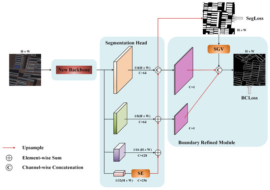
Figure 2.
The overall pipeline of the proposed high-resolution boundary refined network (HBRNet) for AGs detection.
First, the new backbone, a parallel multipath network combining the idea of multiscale grouped convolution and attention mechanism together, is designed and served as a feature extractor, which inherits the advantages of HRNetV2, acquiring multiscale high-layer semantic information while retaining spatial detail information. Second, the segmentation head employs up-sampling and summation operations along the structure from the bottom up to fuse branches after SE module, aiming to rebuild high-resolution feature maps and output segmentation probability maps. Then, the primary boundary mask obtained after SGV operation is fused with the features extracted from the aggregated semantics to generate the finer boundary. Finally, the joint loss integrated by SegLoss and BCLoss is used to supervise the training phase. The resolution and dimension of the feature maps channels are marked as H, W and C in Figure 2. H and W refer to the height and width of input.
3.2. Backbone
In this section, the basic HRNetV2 is firstly introduced and then the PCCA module is described in detail. Finally, we elaborate on two new residual blocks and the novel backbone.
3.2.1. The Basic HRNetV2
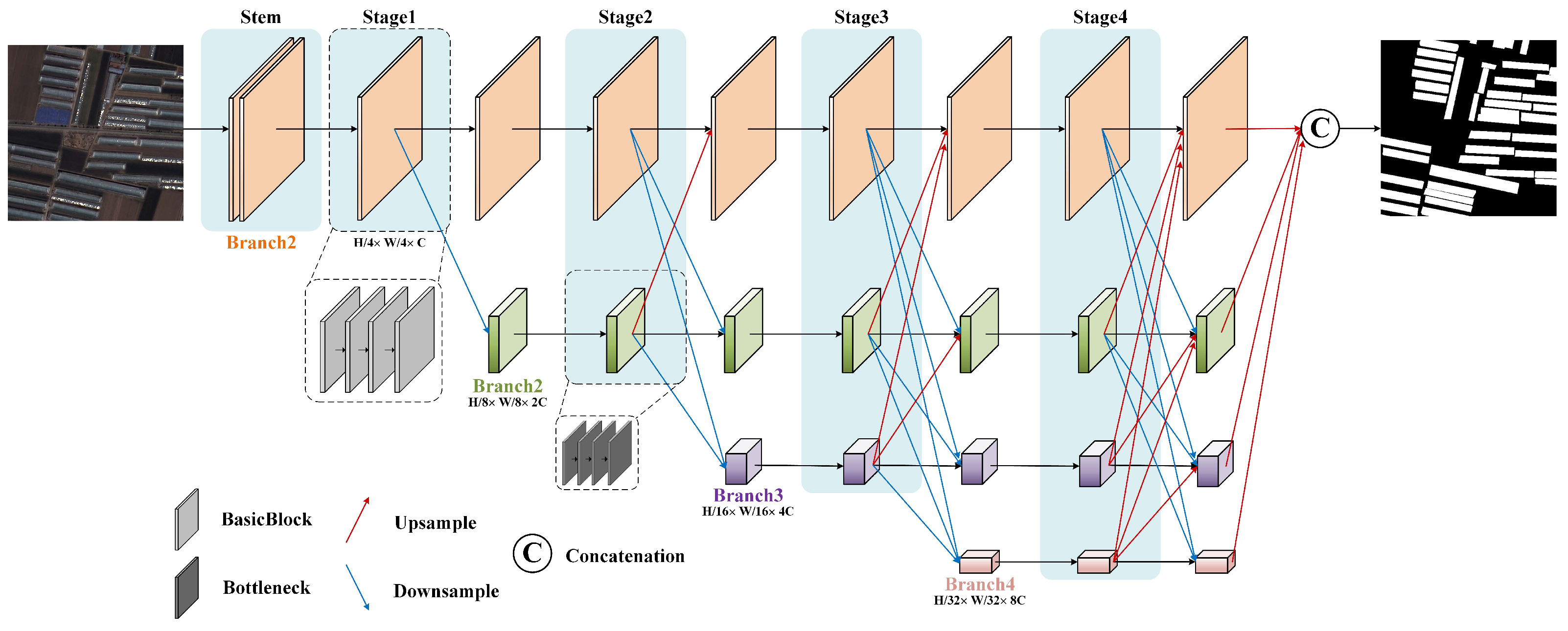
As pictured in Figure 3, HRNetV2 consists of several parallel branches (here four branches) in the architecture corresponding to the gradually descending spatial resolutions. The upper branch can retain a high resolution and preserve the details of spatial information, while the lower branches, gradually added one by one through stride convolution, can obtain richer semantic information benefiting from larger receptive fields. The single resolution feature is acquired by a set of residual blocks in each branch at every stage. Subsequently, the fusion of different branches is realized through a fully connected way so that each resolution can repeatedly get information from others. It is worth nothing that, unlike the basic residual block as the basic element of stage one, all other stages employ the bottleneck block as unit. Finally, the feature maps of all parallel low-resolution subnets are up-sampled to the spatial size of the top branch, then concatenation is employed along the channel dimension to generate the segmentation result. After the input, two 3 × 3 layers with a stride of 2 (see Stem in Figure 3) down-sample the feature map to 1/4 of the original resolution and increase the width (channel number) to C to reduce the memory cost. Therefore, the resolution in different branches decreases to 1/4, 1/8, 1/16 and 1/32 of the original image, and the corresponding width increases to C, 2C, 4C and 8C, respectively.
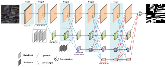
Figure 3.
The structure of basic HRNetV2.
3.2.2. Pyramid Cross Channel Attention Module
The latest research has suggested that the performance for segmentation can be appropriately improved by the attention mechanism [73,74]. Therefore, we drew inspiration from [51,75,76] and developed the PCCA module so as to understand the relevance between multiscale features and to measure the importance of each channel.
As displayed in Figure 4, there are four steps for the execution of the PCCA. First, we can gain multiscale feature maps on all channels through the proposed Pyramid Squeeze Mechanism module (PSM). Secondly, the Channel Attention Mechanism module (CAM) is adopted to extract channel-wise attention vectors of feature maps with different scales. Then, the softmax function is operated on channel-wise attention vectors to generate the whole recalibrated weight, which can be interpreted as a cross channel attention descriptor for all multiscale channels. In the fourth step, the recalibrated weight and corresponding feature map are subjected to an element-wise product and the optimized feature maps with richer scale information will be output.
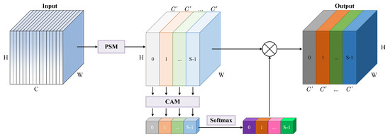
Figure 4.
The structure of the proposed Pyramid Cross Channel Attention module (PCCA).
- Pyramid Squeeze Mechanism Module
The Pyramid Squeeze Mechanism module (PSM), a fundamental operator in the proposed PCCA, is implemented for multiscale feature extraction. As presented in Figure 5, the spatial information of the input feature map is obtained from multiple branches and there are the same number of input channels in each branch.
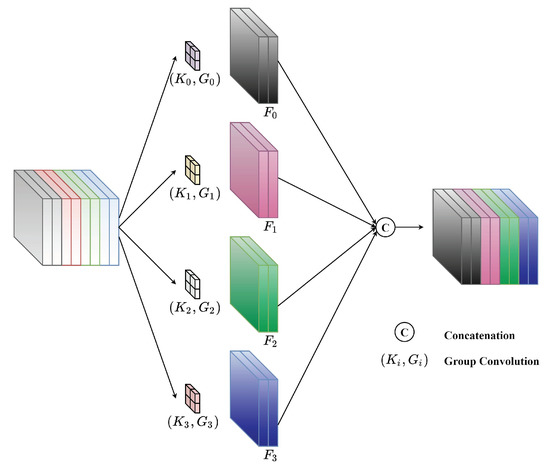
Figure 5.
An example of the Pyramid Squeeze Mechanism module (PSM) with where refers to the kernel size and represents the corresponding group size.
The input features are first squeezed through multiscale convolution kernels and multisize group convolutions in a pyramid structure, and then branches with different scales are obtained. For each branch , the output channel dimension is . Note that must be divisible by .
Specifically, the multiscale feature maps are generated by:
where and indicate the -th kernel size and group size, respectively, and denotes the feature maps with different scales. Furthermore, considering the computational cost, we follow the default settings from the author and employ a novel criterion for selecting the group size and the kernel size without increasing the number of parameters [76]. The relationship between the two can be formulated as:
In our study, is set to 4, so is calculated as 3, 5, 7 and 9 by the formula above, the corresponding are 2, 4, 8 and 16. By employing different kernels to group convolution, the input can be squeezed and multiscale spatial information is learned independently.
- Cross Channel Attention
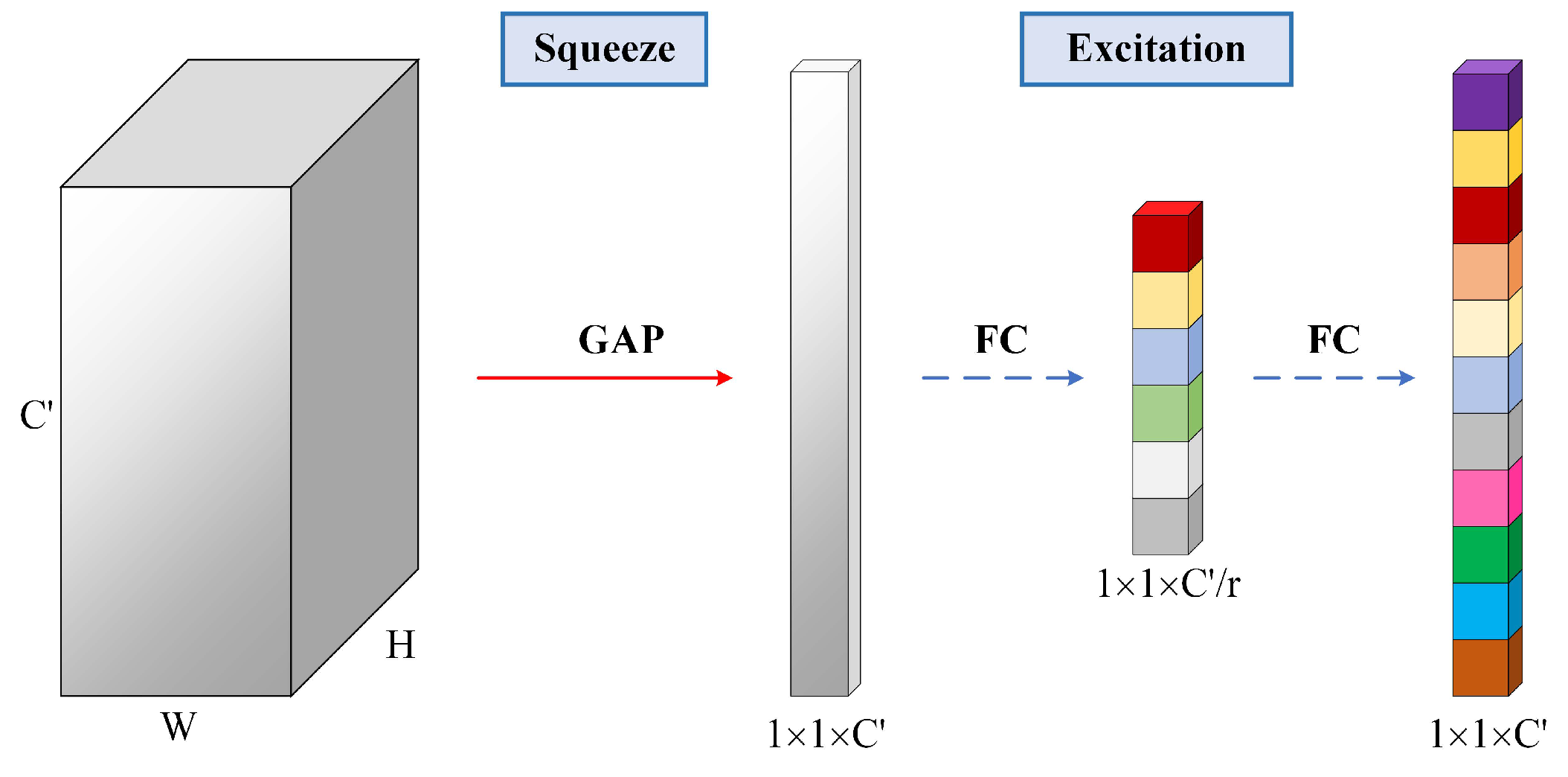
The channel attention mechanism allows the network to increasingly stimulate related channels and suppress fewer effective channels. Therefore, we adopted the Channel Attention Mechanism module (CAM) of SENet [51], which is comprised of squeeze and excitation operations. The diagram is illustrated in Figure 6.

Figure 6.
The Channel Attention Mechanism (CAM) module of SENet.
Firstly, based on the features after PSM module, a channel descriptor is calculated by the global average pooling operation to integrate channel-wise global information. The -th element of can be calculated by the equation:
Then, the excitation operation is implemented for adaptively recalibrating the channel-wise relationship. Formally, the vector of attention weight is defined as:
where is the ReLU [77] function, and refer to two fully-connected layers and represents a sigmoid function. By learning a nonlinear interaction between channels, the attention weight vector with different scales is obtained.
Subsequently, assuming not destroying the original channel attention vector, in order to realize the integration of the cross-dimensions vector and the interaction of attention information, a soft attention mechanism is employed to adaptively select information at different spatial scales, which is under the guidance of the descriptor , as shown in Figure 4. It is given by:
where the re-calibrated weight of all multiscale channels is produced by the softmax function, thus the interaction between local and global channels attention is enabled. Then, the re-calibrated weight of multiscale channel attention is multiplied by the corresponding feature map as:
in which ⊙ denotes channel-wise multiplication and refers to the re-calibrated feature map. Finally, we can generate the refined feature maps by:
where represents the concatenation operation along the channel dimension and represents the whole final output.
Generally, it can be seen from the above reasoning process that the proposed PCCA module can not only integrate spatial information in different scales, but also focuses much on cross channel attention, which can achieve better information interaction between local and global channels.
3.2.3. New Residual Blocks and New Backbone
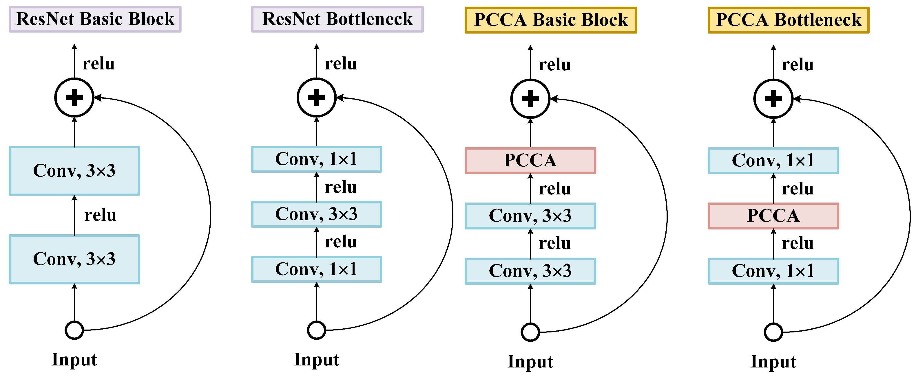
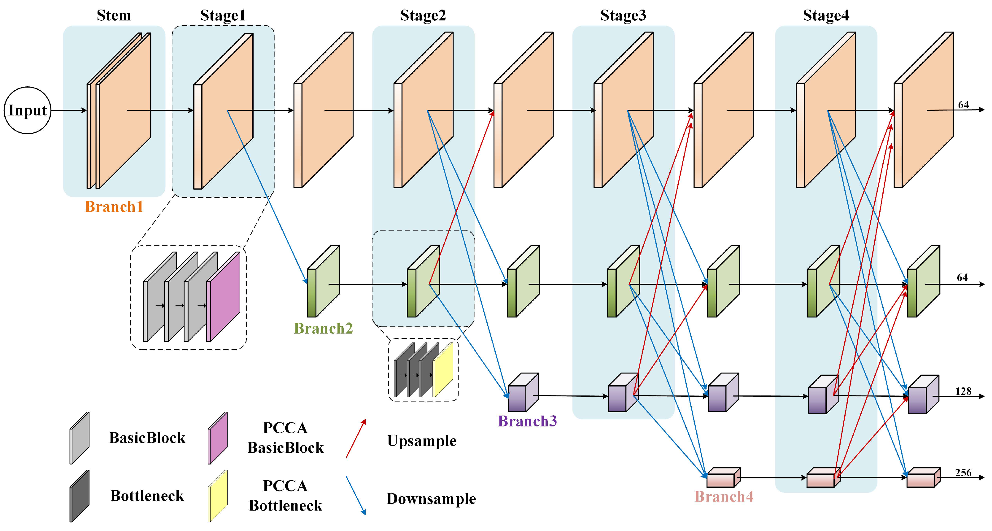
As shown in Figure 7, two brand new blocks named PCCA Basic block and PCCA Bottleneck are proposed and the former adds a PCCA module to the basic block while the latter replaces the 3 × 3 convolution with the PCCA module in the bottleneck of ResNet. Owing to the ability of the PCCA module to integrate multiscale spatial information and cross-channel attention, new residual blocks can extract multiscale spatial information at a finer-grained level and form a long-range channel dependency.

Figure 7.
The architecture of residual blocks. (a) denotes the standard basic block and bottleneck of ResNet and (b) denotes our proposed PCCA basic block and PCCA bottleneck.
Correspondingly, a novel backbone is formed by applying the new proposed residual blocks above to the original HRNetV2. Specifically, different from HRNetV2, the minimum number of residual units (four) are kept in each branch of same stage and the last is replaced with one of the two new units, aiming to make the network lightweight and efficient. Then, we modified the width of the top branch (branch 1) to 64 for high-resolution feature enhancement so as to better restore spatial detail information later. It is worth noting that, referring to the location of the basic unit in HRNetV2, PCCA Basic block is only embedded at stage 1 while PCCA Bottleneck is adopted at the other three stages. Similar to HRNeTv2, there are four parallel branches in the new backbone, and each sub-branch is generated through stride convolution from the upper-branch. The resolution of the feature maps is down-sampled to 1/4 of the original input after Stem. As can be followed from Figure 8, the feature map sizes of the four branches are respectively 1/4, 1/8, 1/16, 1/32 of the input and the corresponding widths are set to 64, 64, 128, 256.
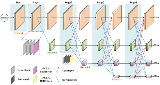
Figure 8.
The architecture of the new backbone.
3.3. Spatial Enchancement Module
As we all know, in complicated scenes, frequent scale changes of AGs result in limited extraction accuracy and problems such as omission of small greenhouses and incomplete large-scale greenhouses often occur. To alleviate this phenomenon, a theoretically ideal context module needed to be designed. Therefore, we developed a unit called Spatial Enhancement (SE) module combining the ideas of dense connection [78] and ASPP [46], which aims to gain denser multiscale features of RSIs. As shown in Figure 9, the SE module is composed of a Dense Cascaded Atrous Spatial Pyramid Pooling (DCASPP), a global encoding module and a skip connection.
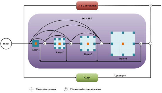
Figure 9.
The structure of the Spatial Enhancement (SE) module.
The global encoding module is implemented through global average pooling operation to generate a representation of the whole feature map, which can effectively prevent overfitting [79]. The skip connection, an element-wise summation followed by a simple 1 × 1 convolution operation, is adopted to take full advantage of high-level semantic features and promote model convergence. The DCASPP uses hybrid multiple cascade 3 × 3 atrous depth-wise separable convolutions [80] with different dilation rates and densely connects them, which can be expressed by the formula:
in which stands for the dilation rate of -th layer, represents the concatenation operation in channel dimension and is the depth-wise separable convolution operation. Note that refers to the input. It has been proved that depth-wise separable convolution can effectively reduce the number of trainable parameters without deteriorating performance [80]. In this paper, the dilation rates are set 1, 2, 3, 5. The RFs calculated by the common ASPP are 3, 5, 7, 11, respectively, while the maximum RF of each layer in the DCASPP can reach 3, 7, 13, 23. DCASPP has the ability to acquire larger RFs and capture denser multiscale contextual information compared to the common ASPP, implying it is more robust to scale changes of AGs.
3.4. Boundary Refined Module
Enlightened by the block designed in [81], we propose the Spatial Gradient Variation (SGV) unit by modifying it, where semantic boundaries of AGs can be easily generated from a segmentation mask by spatial gradient deriving. Herein, adaptive pooling is used to derive spatial gradient :
where represents the position of pixel in the segmentation mask probability map; denotes the absolute value function and is the max-pooling operation with kernel size and stride . The derived boundary width is decided by the parameter . In our study, is set to 3 and to 1.
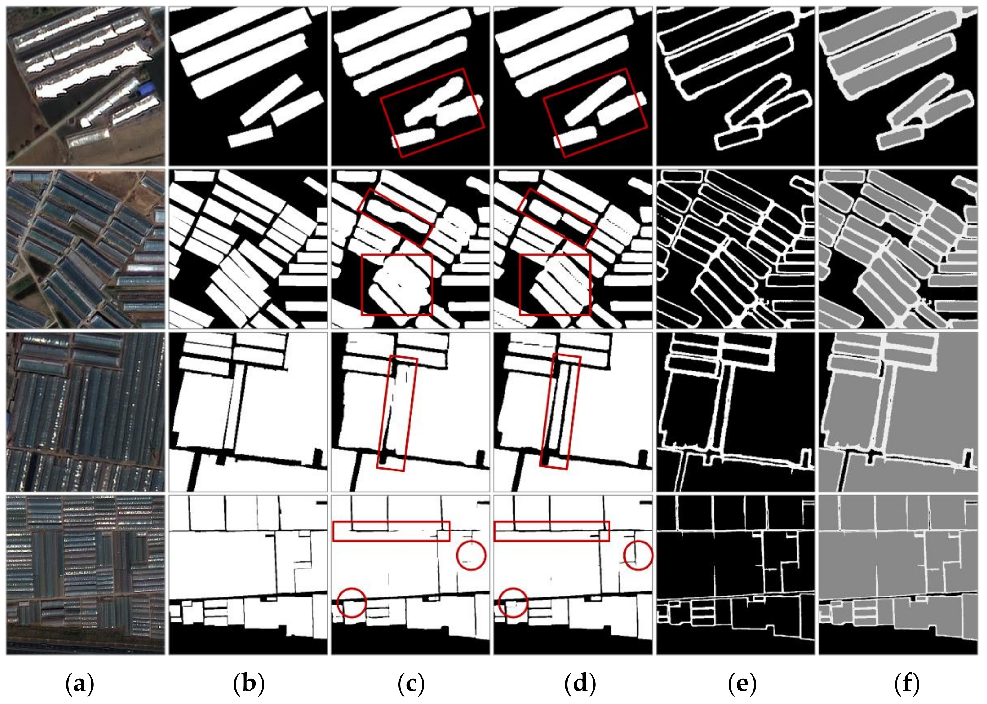
The reason why we use the max-pooling operation instead of the Global Average Pooling (GAP) is that it can produce more precise semantic boundary results. Some examples are shown in Figure 10.
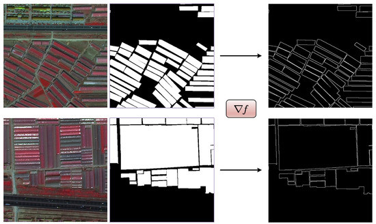
Figure 10.
Typical visualization examples of segmentation masks and derived boundaries through Spatial Gradient Variation (SGV) unit (Column 1 represents the original images in false color composite and the ground truth and boundary are listed in column 2 and column 3, respectively).
As illustrated in Figure 2, in the segmentation head, the feature maps at various resolutions are used to generate the final segmentation probability map combining up-sampling and summation operations. Then, the boundary mask derived from segmentation probability map through SGV is fused in a concatenation way with those single-channel features generated by 1 × 1 convolution, followed by which, the concatenated feature is fed into a convolution layer to finally obtain the boundary probability map. We only choose high-resolution single-channel features from branch 1 and branch 2 (1/4, 1/8 of the input) to better preserve details, which are conducive to boundary extraction.
The SGV module establishes a prototype for boundary extraction, while the derived boundary serves as the constraint for segmentation learning. Compared with independent segmentation and boundary detection, the two tasks can interact with and benefit from each other, so the training becomes easier.
3.5. Loss Functions
As is shown in Figure 2, both segmentation and boundary probability maps are generated from our proposed network. Accordingly, we put forward two loss functions for different tasks.
SegLoss: The standard cross-entropy loss, referred to as , is most commonly adopted in semantic segmentation, which treats each pixel equally. We apply it to segmentation task and compute as follows:
BCLoss: Considering the ambiguity and sparsity of pixels around the boundary, boundary extraction suffers from a higher missing rate. Obviously, it is unreasonable to treat each pixel equally. In order to mitigate this effect, the following class-balanced cross-entropy loss function named is employed, drawing inspiration from [82,83,84]:
Joint loss: Therefore, we couple SegLoss with BCLoss and finally propose the joint loss function as the following formula:
in which stands for a weight parameter for measuring the contribution of BCLoss. In this paper, we tested four different values including 0.5, 1, 2, 5 and the results prove setting it to 2 is the best choice. In this way, the boundary mask can perform auxiliary supervision for the segmentation task of AGs.
4. Experiments
In this section, we present the experiments of our study, i.e., experimental details in Section 4.1, evaluation metric in Section 4.2, comparison to SOTA studies in Section 4.3 and mapping of study area in Section 4.4.
4.1. Experimental Details
Configurations: The proposed network was implemented using Pytorch1.1 framework in the Ubuntu 18.04.5LTS environment. All work was performed on a single NVIDIA GTX TITAN X GPU with 12G memory.
Training Settings: For optimization, the Adam optimizer [85] with an initial learning rate 0.001 () was chosen for training, where weight decay was set to default as recommended. We adopted an exponential weight-decay strategy with a decay rate of 0.9 to adjust the learning rate for each epoch formulated as (). In our study, all models for comparison were trained from scratch for about 50 epochs up to convergence. In view of the limitation of GPU memory, the batch size was set to 4 and same parameter settings were guaranteed to equally evaluate the performance of different approaches.
Dataset settings: Given the risk of overfitting, we apply some common data augmentation methods on each image of 512 × 512 pixels, such as vertical–horizontal flipping and random rotation within a range of [90, 180, 270]. In addition, the pixel values were rescaled between 0 and 1 before being fed into networks.
Inference settings: In the inference phase, the flipping inference strategy was used for evaluation, so we can get final results by averaging all predictions.
4.2. Evaluation Metric
To objectively evaluate the performance of HBRNet and other methods, four common pixel-level metrics consisting of precision, recall, score and Intersection over Union (IoU), were used in our experiments. The precision and recall are formulated as follows:
where , and represent the number of correctly detected AGs pixels (true positives), missed AGs pixels (false positives) and falsely classified background pixels (false negatives), respectively. Precision means the proportion of in all positive predictions, while recall represents the proportion of on all positive samples. Based on them, the score and IoU are expressed as below:
where the former is the weighted average of the precision and recall and the latter calculates the ratio that AGs pixels are correctly recognized.
4.3. Comparison to SOTA Studies
In this section, we illustrate the quantitative comparisons in Section 4.3.1 and then Section 4.3.2 provides the visualization results.
4.3.1. Quantitative Comparisons
To demonstrate the effectiveness of the proposed network, we conducted contrastive experiments on an AG dataset to compare HBRNet with several recent SOTA methods for semantic segmentation in the computer vision community, including FCN8s, UNet, SegNet, PSPNet, DeepLabV3+ and HRNetV2.
Table 2 exhibits the quantitative comparisons of various algorithms with the best results highlighted in bold. According to the results, our proposed HBRNet shows a great improvement and outperforms other SOTA methods in all metrics on the AG dataset. We can clearly observe that the IoU score has been improved by 1.93% over the latest model HRNetV2, which showed the second-best performance. Especially, the proposed approach obtains approximately 4.41%, 10.77%, 7.7% and 13.6% improvement in precision, re-call, score and IoU, compared with FCN8s, and achieves 97.22%, 97.53%, 97.38% and 94.89%, respectively. The near-perfect performance demonstrates that our HBRNet has enough robustness to be applied for AG extraction of RSIs with complex scenarios.

Table 2.
Quantitative comparison (%) vs. SOTA methods on the AG dataset. The records in bold represent the best on the test set.
Furthermore, we compared our method with some recent research including ResUNet [86], LANet [87], MAP-Net [88] and GSCA-UNet [89]. These algorithms all focus on the recognition of various kinds of ground objects in RSIs, which has a certain similarity with AGs extraction and, for fairness, they were reproduced in the same framework.
ResUNet combined advantages of residual learning and UNet. MAP-Net generated multiscale features by a modified multipath neural network and obtained global dependency through a pyramid spatial pooling module to exactly extract building footprints, achieving an IoU accuracy of 90.86% on the WHU datasets. LaNet introduced two light modules including Patch Attention Module (PAM) and Attention Embedding Module (AEM) on the basis of FCN, which aims at tackling the gap between low and high features and improves the precision of segmentation. GASC-UNet developed a global spatial context attention (GSCA) module and embedded it into the U-shaped structure of the encoder and decoder network to adaptively aggregate the global context information of each pixel in the spatial dimension. A better balance was achieved between automation and accuracy.
The segmentation results are reported in Table 3 and the best entries are marked in bold. As we have seen, compared with these approaches, our HBRNet achieves the best performance. Especially, Score metric and IoU metric are boosted by 1.43% and 2.67%, respectively, slightly over the second-best MAP-Net.

Table 3.
Quantitative comparison (%) vs. several other methods on the AG dataset. The best performance are marked as bold.
4.3.2. Visualization Results
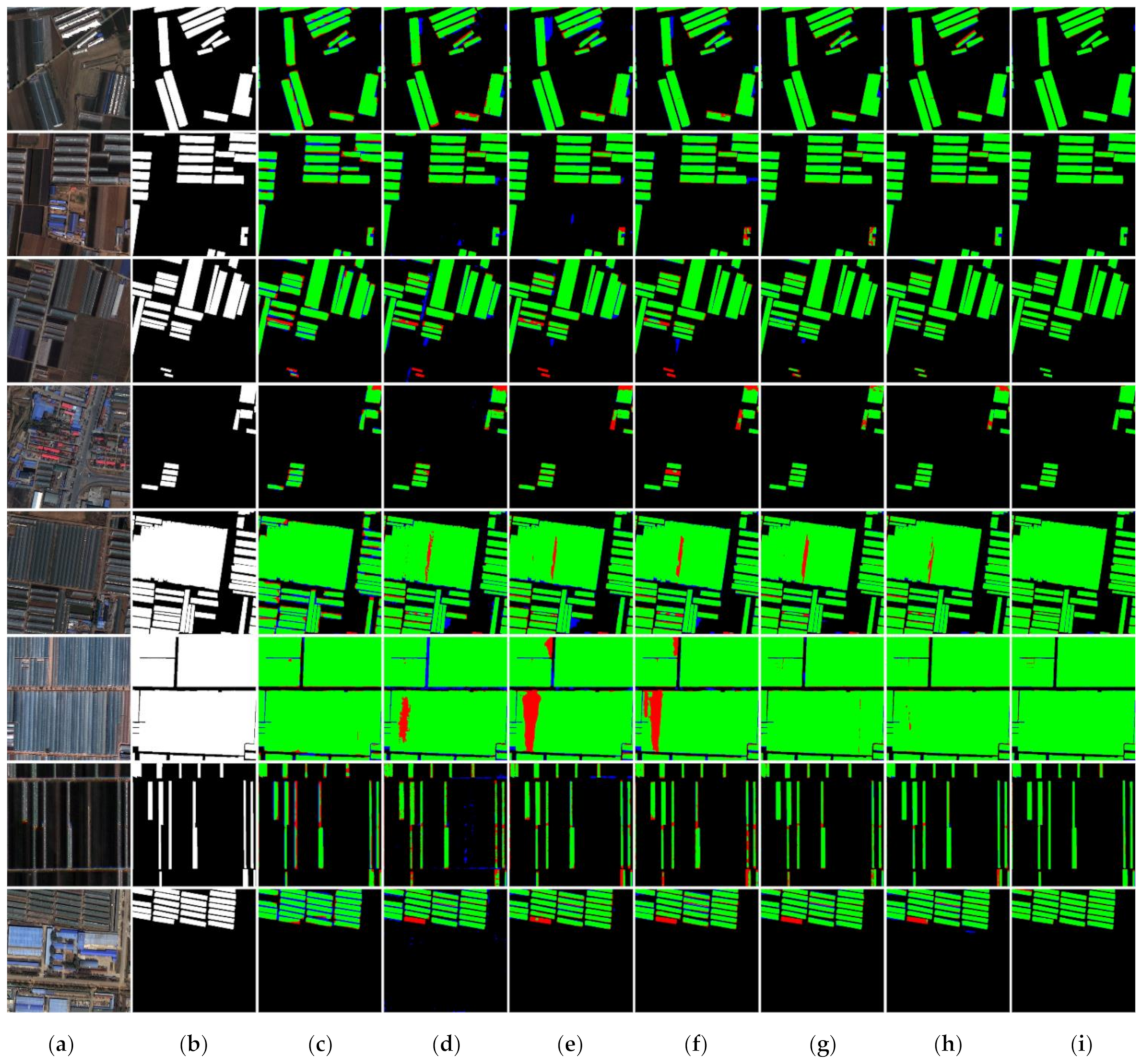
To visually compare different methods, we display some sample results in Figure 11. There are seven examples including AGs with a variety of scales and appearances listed in seven rows. Obviously, compared with other SOTA approaches, HBRNet obtained the most consistent results with ground truth and has strong robustness for greenhouse identification in different complex scenarios. On the contrary, the generalization capacity of other methods is insufficient.
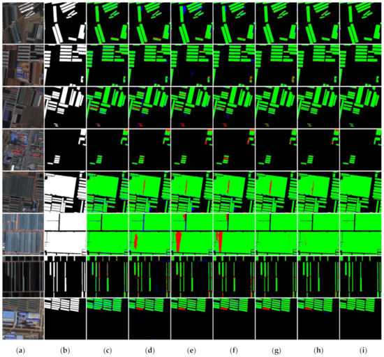
Figure 11.
Examples of AG extraction results produced by multiple approaches. (a) Original image; (b) Ground truth; (c) FCN; (d) SegNet; (e) PSPNet; (f) DeepLabV3+; (g) UNet; (h) HRNetV2; (i) HBRNet. Notably in column (c–i), green, blue and red stand for true positive, false negative and false positive, respectively.
On the whole, FCN shows the poorest performance. As presented in Figure 11c, there exist numerous errors in AG extraction results, which is mainly due to the loss of spatial information through down-sampling operation. Owing to noise introduced from coarse low-level feature maps, SegNet produces blurred and jagged edges, implying the boundary localization is not sufficiently accurate. Meanwhile, “salt and pepper noise” always appears in the results. A striking illustration is listed in the last row of Figure 11d, where parts of farmland and roads are confused as AGs. Compared with the two models above, PSPNet, DeepLabV3+ and UNet gained better segmentation performance and all obtained a reasonable result in a simple scenario. However, with more diverse AGs and more complex scenes, parts were misclassified or missed. For example, it can be clearly observed that small greenhouses suffer a high miss rate according to the third and fourth row in Figure 11 and large greenhouses are always incompletely extracted and holey, as displayed in the fifth and sixth row, suggesting that these methods are sensitive to the variation of scales and difficult to accurately recognize as AGs. Benefiting from multibranch parallel architecture, HRNetV2 can easily reserve spatial details, which means the integrity of AGs of various scales can be maintained to some extent. Nevertheless, the effect of edge extraction is not ideal. We realize that AGs with irregular structure may contain multiple corners, and HRNetV2 cannot correctly distinguish other adjacent pixels with similar features, possibly contributing to over-extraction (see the first and second row of Figure 11h).
Despite the gradual progress, these classic semantic segmentation algorithms have their own limitations and shortcomings. On the contrary, HBRNet combines three improved modules including the PCCA, SE and BR module, which respectively strengthen the interpretation capability of the network, overcome multiscale identification problems, reduce the probability of omission and misrecognition and provide simple but effective solutions for edge problems. As shown in Figure 11i, our method not only obtains the best extraction results but restores the geometric shape and spatial distribution of AGs to the greatest extent, which verifies its superiority and accuracy.
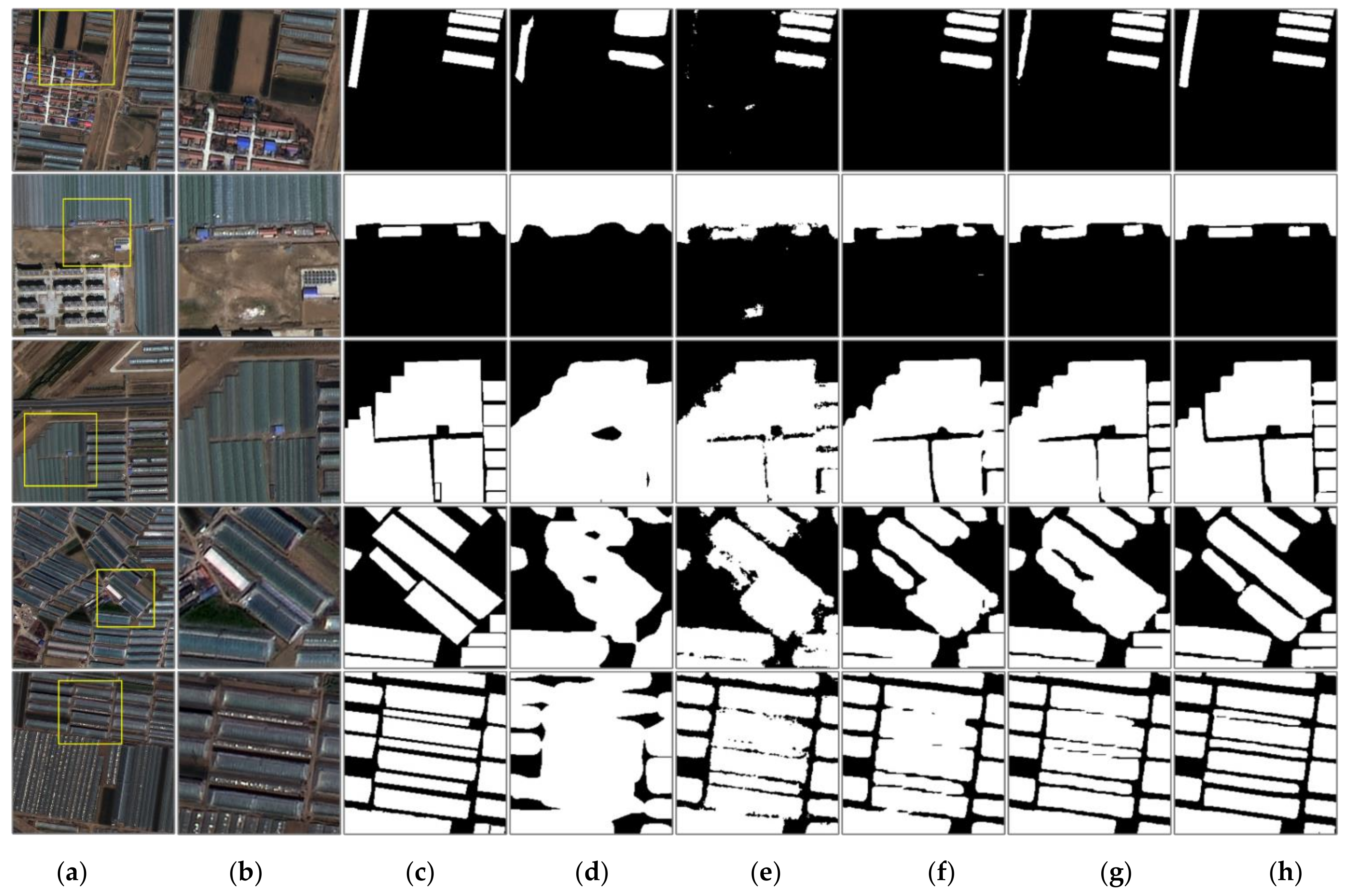
To demonstrate the details clearly, Figure 12 presents the results of typical areas on the images in a closer perspective, circled by the yellow rectangle. We chose representative models including FCN, SegNet, PSPNet, HRNetV2 and our HBRNet for comparison.
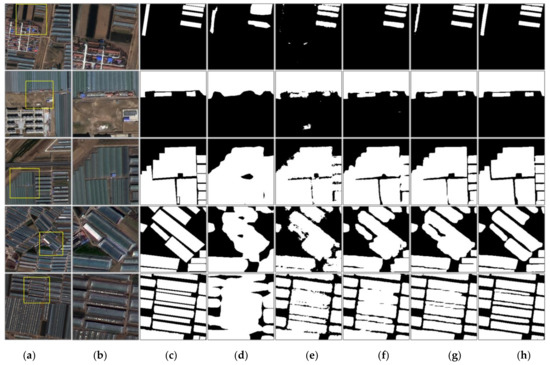
Figure 12.
Results extracted by part of the SOTA methods in a closer perspective. Images and results presented in column (b–h) correspond to the selected regions circled by the yellow rectangle in (a). (a) Original image. (b) Image of typical area. (c) Ground truth; (d) FCN; (e) SegNet; (f) PSPNet; (g) HRNetV2; (h) Ours.
From close observation, we can find:
- Our network can detect all AGs more comprehensively than other approaches. As presented in the first row of Figure 12, AGs with inconspicuous characteristics were successfully identified and plastic film mulch with similar spectral response could be separated, implying that the proposed model has been equipped with strong feature extraction capability, which is superior to other methods.
- We can see from the segmentation results that it is difficult for other SOTA methods to distinguish the easily confused adjacent non-greenhouse objects. Especially, as displayed in the middle columns in Figure 12, “adhesion” phenomena usually appear, that is, the background between AGs distributed more densely can be easily misidentified as greenhouse because of a short distance, thus AGs existing as independent individuals cannot be recognized correctly. However, boundary supervision implemented through the joint of the BR module and BCloss in our network can alleviate the indistinguishability and present the truth, as can be seen from the last column in Figure 12.
- The geometric shapes of AGs are diverse, most of which are rectangular or irregular blocks, and the boundaries always contain multiple straight lines and right-angles. Because other approaches cannot accurately locate positions, the edges extracted appear curved, which is not consistent with the label. However, HBRNet can generate a smoother boundary and basically maintain the geometrical morphology of AGs. This should be attributed to the BR module which revised the segmentation results in the later stage and refined the precision of the boundary (typical examples can be found in the second and third rows).
4.4. Mapping of Study Area
Compared with natural images, RSIs have huge data magnitudes. The size of an orthorectified GF-2 image is more than 30,000 × 30,000 pixels, which greatly exceeds the 512 × 512 size of patches used in the training process. As mentioned in the previous section, the sufficiency of contextual information affects segmentation performance, which suggests that pixels close to the edge cannot be classified as confidently as ones close to the center, because the lack of information outside the patch limits the contextual information of the edge region. There may appear stitching traces if a regular grid is adopted for cropping, predicting and mosaicking.
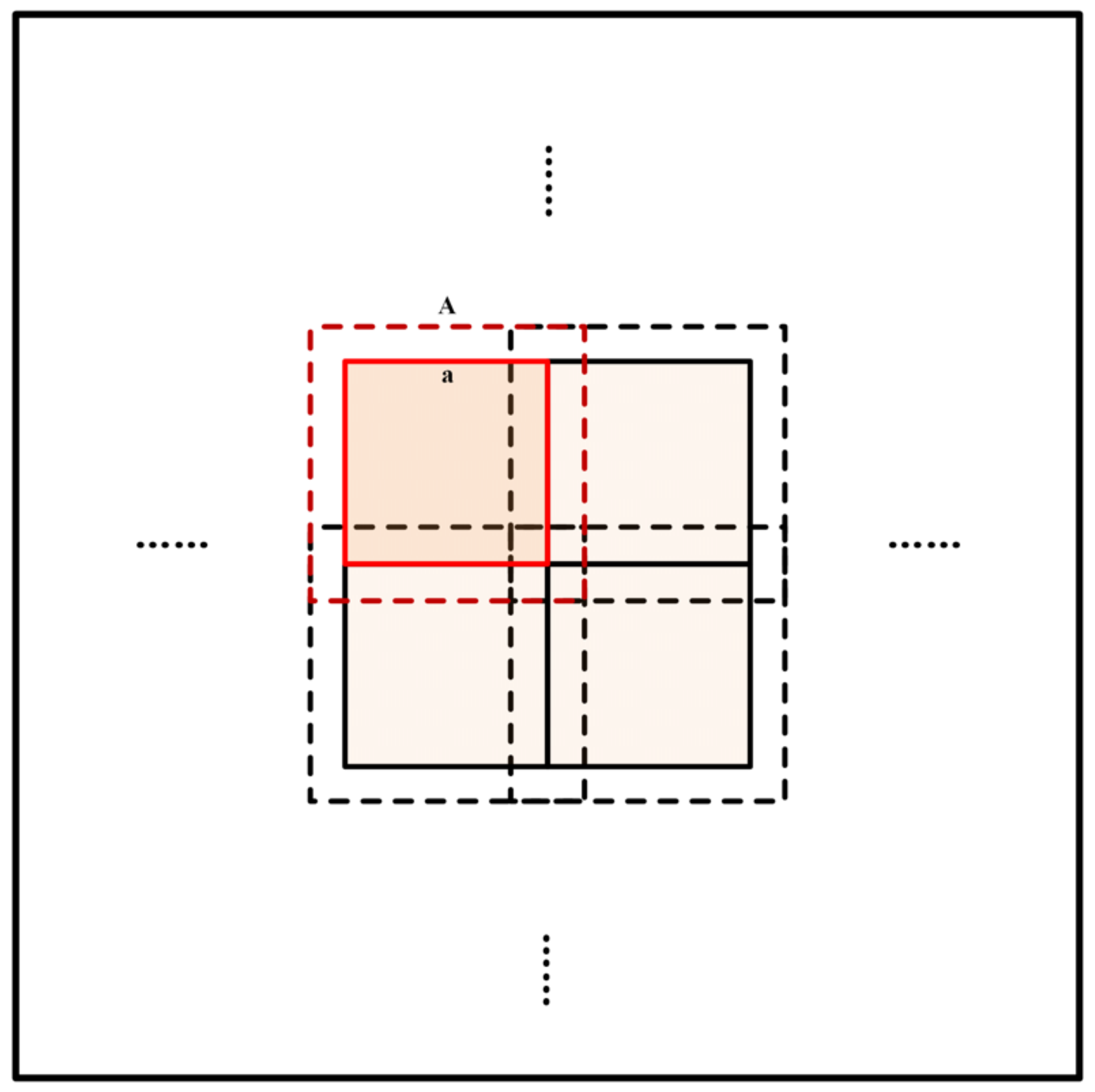
To further improve the segmentation performance and obtain smooth masks, we adopt the strategy of edge-ignoring prediction, that is, employing the sliding window to crop the image with overlapping and ignoring part of the edge area during the mosaicking. As shown in Figure 13, the actual prediction result of cropped patch has a size of A × A, yet the final size used for stitching is a × a.
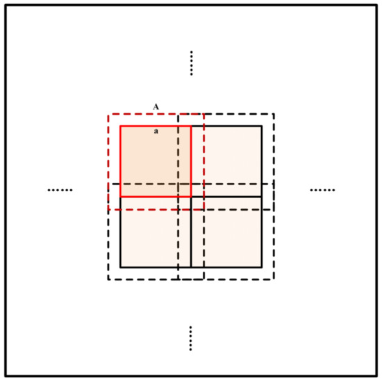
Figure 13.
The strategy of edge-ignoring prediction.
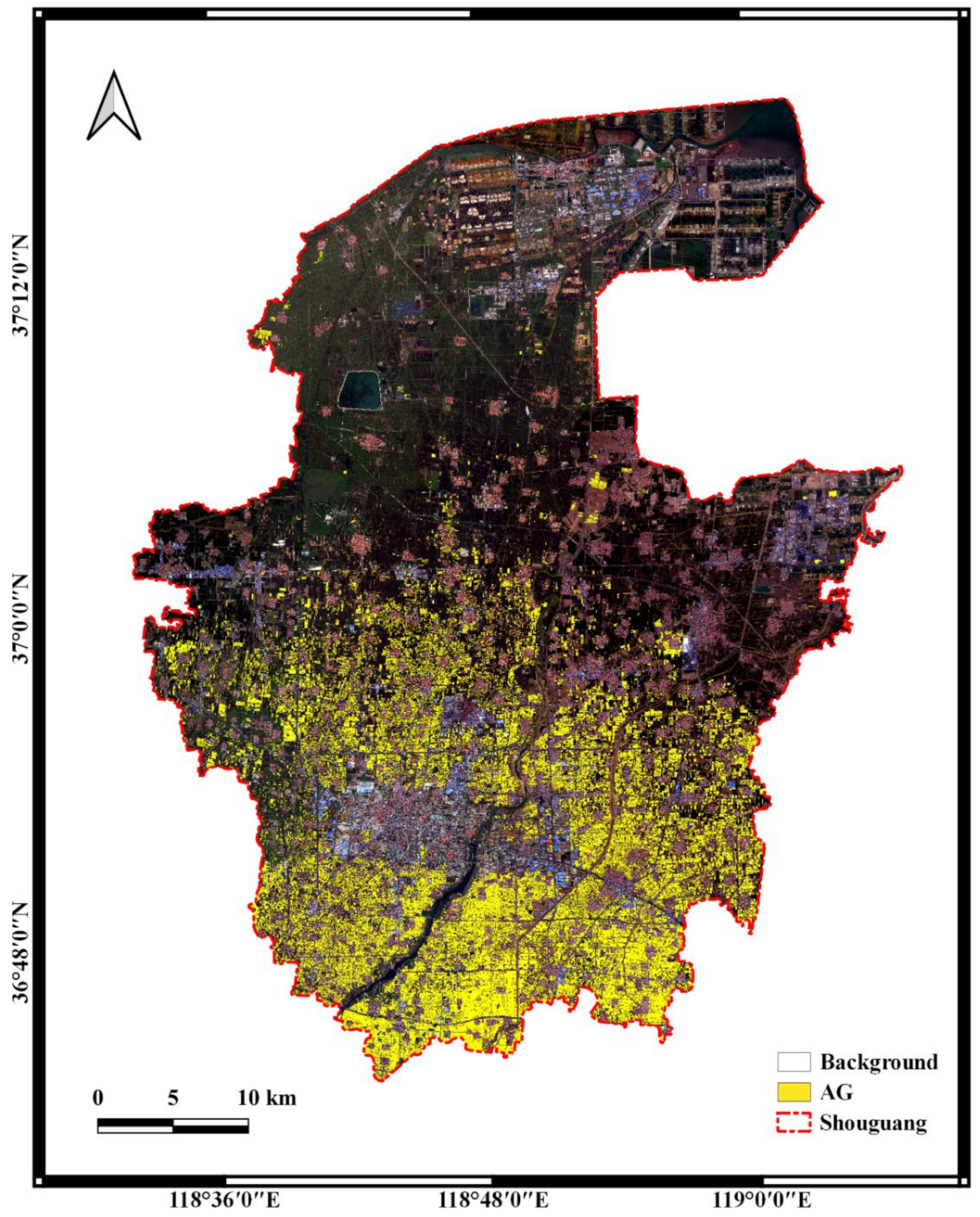
In our experiment, the size of the sliding window is 512 × 512 and the number of edge pixels ignored in the four directions of the patch is 56. In other words, the 400 × 400 square part centrally is used for stitching. Finally, we mosaic multiple segmentation masks to obtain the distribution mapping of the entire study area. As presented in Figure 14, we can observe that the south is a concentrated district of AGs in Shouguang while it is relatively sparse in the north, implying that our method can identify AGs in different scenarios, which is applicable for large-scale automated mapping.

Figure 14.
The distribution map of AGs in Shouguang District.
5. Discussion
In this section, the comparative experiment is firstly used to verify the generalization of the BR module and then we analyze the roles of each proposed module. Finally, the complexity analysis of related methods and the limitations of our method are discussed.
5.1. Effectiveness of the Boundary Refined Module
To verify the generalization of the BR module, we applied it to UNet and the corresponding BCLoss was also introduced for training. According to records in Table 4, whether embedded in UNet or in our framework, this module can improve the performance with little increase in computational cost. The comparison results strongly demonstrate its effectiveness and certain applicability. Note that the flipping inference strategy is not adopted in this contrast experiment.

Table 4.
Comparison of performance by only SegLoss and the Joint Loss; the difference is whether BR module was employed in UNet or HBRNet. ✓ means the corresponding component is adopted.
As mentioned in Section 3.5, the proposed joint loss function may affect the segmentation performance; to further investigate the contribution of the boundary auxiliary task, we used different joint loss functions with varying weight in Equation (12) to train HBRNet on the AG dataset. The network was trained eventually to get five sets of results in total, four for AGs extraction and boundary detection simultaneously and the remaining one for only AGs extraction task. All training processes took 50 epochs to converge and the performances with different parameter configurations are displayed in Table 5.

Table 5.
Comparison of networks with different joint loss functions varying in weight on the AG dataset. λi = 0 denotes that the network only implements segmentation task. The best entries are highlighted in bold.
The weight decides how much the network focuses on the edge and the degree of emphasis increases as grows. Table 5 clearly shows that no matter what the value is set to, our approach can obtain better results on all metrics with the auxiliary constraint of boundary learning. Figure 15 also proves that the network with boundary learning is beneficial to maintain the morphological characteristics of AGs, with more complete edge, clearer straight and right angles and fewer misclassified pixels. However, we find that a too big or too small value can affect the stability of performance, so for a tradeoff, it is recommended to set this parameter to 2 to maximize the overall performance.

Figure 15.
Examples of AG identification results differ whether the BR module participates in training. From left to right: (a) Original image. (b) Ground truth. (c) Prediction by only segmentation task. (d) Prediction by the joint of segmentation task and boundary learning (). (e) Boundary prediction; (f) Combination of two predictions.
5.2. Ablation Experiments
For the purpose of analyzing the roles of different modules of HBRNet, ablation studies were conducted on the AG dataset and we adopted precision, recall, Score and IoU for evaluation. The ablation experimental results are shown in Table 6 with the best entries highlighted in bold.

Table 6.
Ablation experiments for the network design, where HRNetV2 serves as baseline. ✓ means the corresponding component is adopted.
First, based on the baseline HRNetV2, the new backbone described in Section 3.2 was applied to optimize its structure. The modified framework, with a fusion operation at the end that was the same as in HRNetV2, outperforms HRNeV2 by 0.67%., which is contributed to by the powerful feature extraction capability of the PCCA module. Then, after embedding the SE module in the segmentation head to capture multiscale information, the IoU is improved by 0.18%, indicating that SE is robust in addressing crucial scale issues for AG objects. Finally, as expected, compared only with the segmentation task, the combination of boundary extraction and the BCLoss function boosted the IoU performance by 0.83%; and, furthermore, with the assistance of flipping inference strategy, our proposed method achieves a 94.89% IoU, which is a 1.93% arise compared to the baseline.
5.3. Complexity Analysis
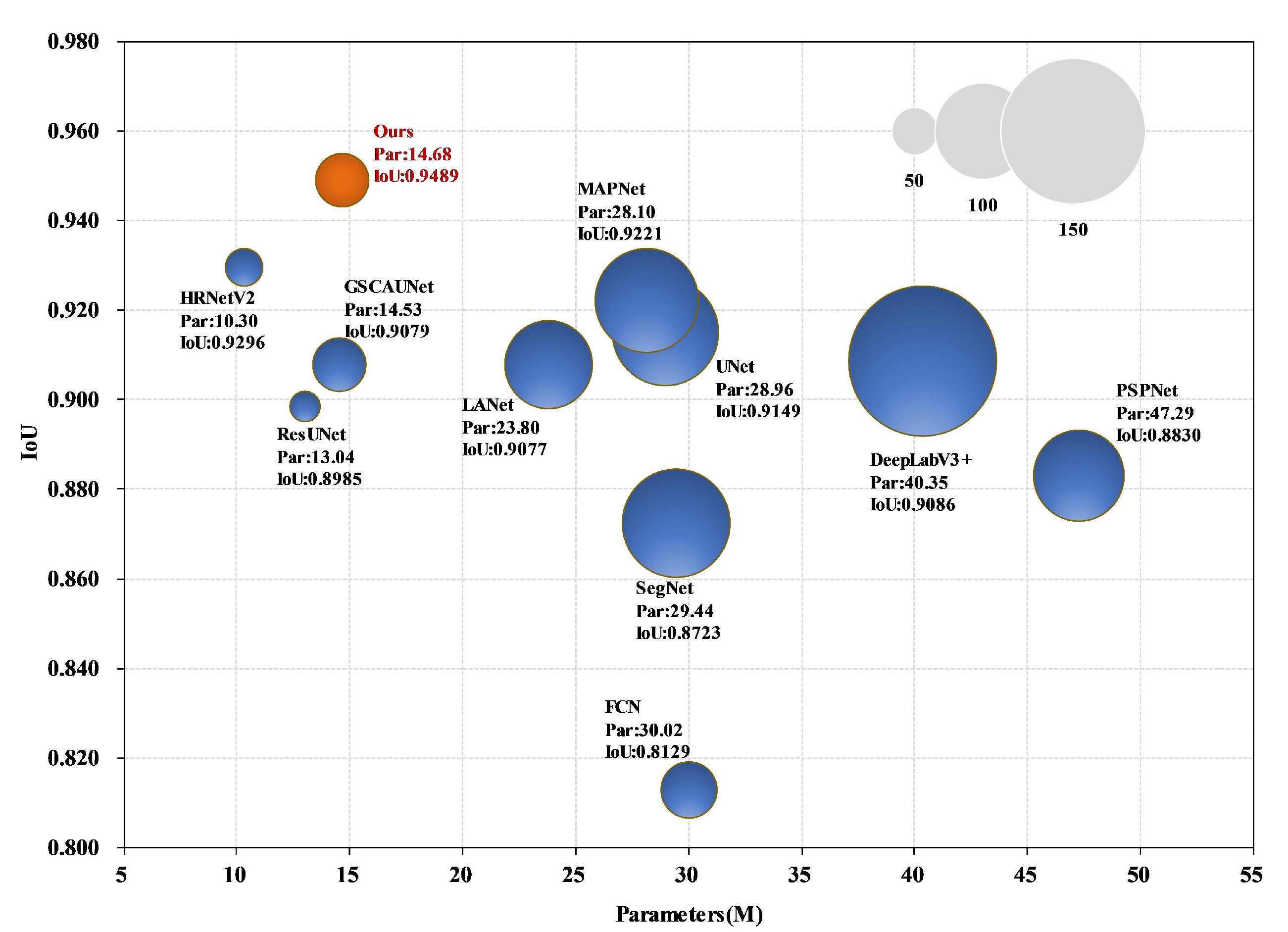
Our proposed approach adopts a parallel multipath structure; some branches are needed to process high-resolution feature maps to maintain accurate localization information, which may result in a mass of parameters. To verify the tradeoff between the complexity and performance of HBRNet, three indexes including parameter, FLOPs and IoU of related algorithms are compared on the AG dataset.
As presented in Table 7, HRNetV2 contains the fewest parameters but relatively lower extraction accuracy. Due to a large number of convolution operations, PSPNet and DeeplabV3+ with ResNet50 as encoder have higher complexity, whereas their performance is poor. The reasonable explanation is that its decoder structure does not rebuild high resolution feature maps step by step. It is also clearly observed that ResUNet has a small number of parameters but still numerous FLOPs, which poses more requirements for hardware.

Table 7.
Comparison of related algorithms on parameters, FLOPs and IoU on the AG dataset. The fewest parameters, smallest FLOPs and highest IoU are marked in bold.
After the redesign of the backbone and introduction of SE module and BR module, the complexity of HBRNet slightly increased based on HRNetV2; however, compared with other methods, better performance was achieved with far fewer parameters.
To visually compare the complexity and performance, we display the experimental results on a scatter plot as shown in Figure 16, in which diameter of blue circle denotes the size of the model file and the number of parameters and IoU metric stand for the complexity and accuracy of each other method. It can be concluded that compared with other related methods, our proposed HBRNet maintains the highest accuracy and relatively lower complexity.

Figure 16.
Comparison of complexity and performance obtained by different methods. IoU and the number of parameters of each approach are marked.
6. Conclusions
Effective and accurate AG extraction is crucial to monitor the distribution and estimate coverage of AGs. However, due to diverse geometric appearances and different spectral features, traditional semantic segmentation has limited accuracy and inaccurate boundary localization. Therefore, we set up an AG dataset and a novel framework named HBRNet was proposed to conduct experiments on this dataset. In this method, the PCCA module was introduced into a parallel multibranch architecture to form a new backbone. While maintaining high-resolution detailed information, it also recalibrated the contribution of each channel through cross channel attention, enhancing its capability of feature extraction. Furthermore, the SE module further rebuilds and optimizes features in the space domain and thus the network can attach more importance to small-size greenhouses and restrain the holes that appear on the larger scale. In particular, the BR module was combined with the BCLoss to prompt the model to pay more attention to the pixel classification around the boundary. The comprehensive experiments demonstrated that our method outperforms other typical semantic segmentation approaches in performance with relatively less complexity. In addition, we conducted ablation experiments to evaluate the consequences of each proposed module. Although a small number of parameters cost less memory, our HBRNet is relatively inefficient because of the existence of group convolution. In future research, we will further improve our algorithm in computational efficiency towards a lighter convolution structure. Our current experiments mainly focus on AG extraction and we hope it will be employed to various target recognition tasks such as building and aquaculture areas to verify its applicability.
Author Contributions
X.Z. designed the experiments and wrote the manuscript. B.C. provided the original data, supervised the study and reviewed the draft paper. C.L. and J.C. revised the manuscript and gave some appropriate suggestions. All authors have read and agreed to the published version of the manuscript.
Funding
This research was funded by the National Natural Science Foundation of China (61731022, 61860206004).
Institutional Review Board Statement
Not applicable.
Informed Consent Statement
Not applicable.
Data Availability Statement
Not applicable.
Acknowledgments
This work was partially funded by the National Natural Science Foundation of China (61731022, 61860206004) and the Strategic Priority Research Program of the Chinese Academy of Sciences (Grant Numbers XDA19010401). The authors also thank the anonymous reviewers and the editors for their insightful comments and helpful suggestions to improve our manuscript.
Conflicts of Interest
The authors declare no conflict of interest.
Abbreviations
The following abbreviations are used in this manuscript:
| HBRNet | High-Resolution Boundary Refined Network |
| AGs | Agricultural Greenhouses |
| DCNN | Deep Convolutional Neural Network |
| PCCA | Pyramid Cross Channel Attention |
| SE | Spatial Enhancement |
| SGV | Spatial Gradient Variation |
| BR | Boundary Refined |
| RSIs | Remote Sensing images |
| FCN | Fully Convolutional Network |
| SegLoss | Segmentation Loss |
| BCLoss | Boundary Constraint Loss |
| DCASPP | Dense Cascaded Atrous Spatial Pyramid Pooling |
| SGV | Spatial Gradient Variation |
| PSM | Pyramid Squeeze Mechanism |
| CAM | Channel Attention Mechanism |
| IoU | Intersection over Union |
References
- Cantliffe, D.J. Protected agriculture—A regional solution for water scarcity and production of high-value crops in the Jordan Valley. In Proceedings of the Water in the Jordan Valley: Technical Solutions and Regional Cooperation Conference, Norman, OK, USA, 13–14 November 2001; pp. 13–14. [Google Scholar]
- Levin, N.; Lugassi, R.; Ramon, U.; Braun, O.; Ben-Dor, E. Remote sensing as a tool for monitoring plasticulture in agricultural landscapes. Int. J. Remote. Sens. 2007, 28, 183–202. [Google Scholar] [CrossRef]
- Picuno, P.; Tortora, A.; Capobianco, R.L. Analysis of plasticulture landscapes in Southern Italy through remote sensing and solid modelling techniques. Landsc. Urban Plan. 2011, 100, 45–56. [Google Scholar] [CrossRef]
- Picuno, P. Innovative material and improved technical design for a sustainable exploitation of agricultural plastic film. Polym.-Plast. Technol. Eng. 2014, 53, 1000–1011. [Google Scholar] [CrossRef]
- González-Yebra, Ó.; Aguilar, M.A.; Nemmaoui, A.; Aguilar, F.J. Methodological proposal to assess plastic greenhouses land cover change from the combination of archival aerial orthoimages and Landsat data. Biosyst. Eng. 2018, 175, 36–51. [Google Scholar] [CrossRef]
- Garnaud, J. “Plasticulture” magazine: A milestone for a history of progress in plasticulture. Plasticulture 2000, 1, 30–43. [Google Scholar]
- Briassoulis, D.; Dougka, G.; Dimakogianni, D.; Vayas, I. Analysis of the collapse of a greenhouse with vaulted roof. Biosyst. Eng. 2016, 151, 495–509. [Google Scholar] [CrossRef]
- Aguilar, M.A.; Bianconi, F.; Aguilar, F.J.; Fernández, I. Object-Based Greenhouse Classification from GeoEye-1 and WorldView-2 Stereo Imagery. Remote. Sens. 2014, 6, 3554–3582. [Google Scholar] [CrossRef] [Green Version]
- Chaofan, W.; Jinsong, D.; Ke, W.; Ligang, M.; Tahmassebi, A.R.S. Object-based classification approach for greenhouse mapping using Landsat-8 imagery. Int. J. Agric. Biol. Eng. 2016, 9, 79–88. [Google Scholar] [CrossRef]
- National Bureau of Statistics. Communiqué on Major Data of the Third National Agricultural Census (No. 2). Available online: http://www.stats.gov.cn/tjsj/tjgb/nypcgb/qgnypcgb/201712/t20171215_1563539.html (accessed on 15 December 2017).
- Sica, C.; Picuno, P. Spectro-radiometrical characterization of plastic nets for protected cultivation. In Proceedings of the International Symposium on High Technology for Greenhouse System Management: Greensys, Naples, Italy, 4–6 October 2007; pp. 245–252. [Google Scholar]
- Picuno, P.; Sica, C.; Laviano, R.; Dimitrijević, A.; Scarascia-Mugnozza, G. Experimental tests and technical characteristics of regenerated films from agricultural plastics. Polym. Degrad. Stab. 2012, 97, 1654–1661. [Google Scholar] [CrossRef]
- Knickel, K. Changes in Farming Systems, Landscape, and Nature: Key Success Factors of Agri-Environmental Schemes (AES); na: 2000. Available online: https://eurekamag.com/research/003/378/003378043.php (accessed on 21 October 2021).
- Du, X.; Wu, Z.; Zhang, Y.; Pei, X. Study on changes of soil salt and nutrient in greenhouse of different planting years. J. Soil Water Conserv. 2007, 2, 78–80. [Google Scholar] [CrossRef]
- Yang, D.; Chen, J.; Zhou, Y.; Chen, X.; Chen, X.; Cao, X. Mapping plastic greenhouse with medium spatial resolution satellite data: Development of a new spectral index. ISPRS J. Photogramm. Remote Sens. 2017, 128, 47–60. [Google Scholar] [CrossRef]
- Xu, Z.; Su, C.; Zhang, X. A semantic segmentation method with category boundary for Land Use and Land Cover (LULC) mapping of Very-High Resolution (VHR) remote sensing image. Int. J. Remote Sens. 2021, 42, 3146–3165. [Google Scholar] [CrossRef]
- Rudorff, N.; Rudorff, C.M.; Kampel, M.; Ortiz, G. Remote sensing monitoring of the impact of a major mining wastewater disaster on the turbidity of the Doce River plume off the eastern Brazilian coast. ISPRS J. Photogramm. Remote Sens. 2018, 145, 349–361. [Google Scholar] [CrossRef]
- Lynch, P.; Blesius, L.; Hines, E. Classification of Urban Area Using Multispectral Indices for Urban Planning. Remote Sens. 2020, 12, 2503. [Google Scholar] [CrossRef]
- Wellmann, T.; Lausch, A.; Andersson, E.; Knapp, S.; Cortinovis, C.; Jache, J.; Scheuer, S.; Kremer, P.; Mascarenhas, A.; Kraemer, R.; et al. Remote sensing in urban planning: Contributions towards ecologically sound policies? Landsc. Urban Plan. 2020, 204, 103921. [Google Scholar] [CrossRef]
- Li, M.; Zhang, Z.; Lei, L.; Wang, X.; Guo, X. Agricultural Greenhouses Detection in High-Resolution Satellite Images Based on Convolutional Neural Networks: Comparison of Faster R-CNN, YOLO v3 and SSD. Sensors 2020, 20, 4938. [Google Scholar] [CrossRef] [PubMed]
- Giri, C.; Pengra, B.; Long, J.; Loveland, T.R. Next generation of global land cover characterization, mapping, and monitoring. Int. J. Appl. Earth Obs. Geoinf. 2013, 25, 30–37. [Google Scholar] [CrossRef]
- Koc-San, D. Evaluation of different classification techniques for the detection of glass and plastic greenhouses from WorldView-2 satellite imagery. J. Appl. Remote Sens. 2013, 7, 073553. [Google Scholar] [CrossRef]
- Lu, L.; Hang, D.; Di, L. Threshold model for detecting transparent plastic-mulched landcover using moderate-resolution imaging spectroradiometer time series data: A case study in southern Xinjiang, China. J. Appl. Remote Sens. 2015, 9, 097094. [Google Scholar] [CrossRef]
- Hasituya; Chen, Z.; Li, F.; Hongmei. Mapping Plastic-Mulched Farmland with C-Band Full Polarization SAR Remote Sensing Data. Remote Sens. 2017, 9, 1264. [Google Scholar] [CrossRef] [Green Version]
- Xu, Y.; Wu, L.; Xie, Z.; Chen, Z. Building Extraction in Very High Resolution Remote Sensing Imagery Using Deep Learning and Guided Filters. Remote Sens. 2018, 10, 144. [Google Scholar] [CrossRef] [Green Version]
- Novelli, A.; Aguilar, M.A.; Nemmaoui, A.; Aguilar, F.J.; Tarantino, E. Performance evaluation of object based greenhouse detection from Sentinel-2 MSI and Landsat 8 OLI data: A case study from Almería (Spain). Int. J. Appl. Earth Obs. Geoinf. 2016, 52, 403–411. [Google Scholar] [CrossRef] [Green Version]
- Balcik, F.B.; Senel, G.; Goksel, C. Greenhouse Mapping using Object Based Classification and Sentinel-2 Satellite Imagery. In Proceedings of the 2019 8th International Conference on Agro-Geoinformatics (Agro-Geoinformatics), Istanbul, Turkey, 16–19 July 2019; pp. 1–5. [Google Scholar]
- Jiménez-Lao, R.; Aguilar, F.J.; Nemmaoui, A.; Aguilar, M.A. Remote Sensing of Agricultural Greenhouses and Plastic-Mulched Farmland: An Analysis of Worldwide Research. Remote Sens. 2020, 12, 2649. [Google Scholar] [CrossRef]
- Wang, C.; Chen, J.; Wu, J.; Tang, Y.; Shi, P.; Black, T.A.; Zhu, K. A snow-free vegetation index for improved monitoring of vegetation spring green-up date in deciduous ecosystems. Remote Sens. Environ. 2017, 196, 1–12. [Google Scholar] [CrossRef]
- LeCun, Y.; Bengio, Y.; Hinton, G. Deep learning. Nature 2015, 521, 436–444. [Google Scholar] [CrossRef]
- Reichstein, M.; Camps-Valls, G.; Stevens, B.; Jung, M.; Denzler, J.; Carvalhais, N. Deep learning and process understanding for data-driven Earth system science. Nature 2019, 566, 195–204. [Google Scholar] [CrossRef]
- Hongtao, L.; Qinchuan, Z. Applications of deep convolutional neural network in computer vision. J. Data Acquis. Process. 2016, 31, 1–17. [Google Scholar] [CrossRef]
- Long, J.; Shelhamer, E.; Darrell, T. Fully convolutional networks for semantic segmentation. In Proceedings of the IEEE Conference on Computer Vision and Pattern Recognition, Boston, MA, USA, 7–12 June 2015; pp. 3431–3440. [Google Scholar]
- Eigen, D.; Fergus, R. Predicting depth, surface normals and semantic labels with a common multi-scale convolutional architecture. In Proceedings of the IEEE International Conference on Computer Vision, Santiago, Chile, 7–13 December 2015; pp. 2650–2658. [Google Scholar]
- Mostajabi, M.; Yadollahpour, P.; Shakhnarovich, G. Feedforward semantic segmentation with zoom-out features. In Proceedings of the IEEE Conference on Computer Vision and Pattern Recognition, Boston, MA, USA, 7–12 June 2015; pp. 3376–3385. [Google Scholar]
- Li, L. Deep Residual Autoencoder with Multiscaling for Semantic Segmentation of Land-Use Images. Remote Sens. 2019, 11, 2142. [Google Scholar] [CrossRef] [Green Version]
- Wang, J.; Ding, C.H.Q.; Chen, S.; He, C.; Luo, B. Semi-Supervised Remote Sensing Image Semantic Segmentation via Consistency Regularization and Average Update of Pseudo-Label. Remote Sens. 2020, 12, 3603. [Google Scholar] [CrossRef]
- Liu, W.; Chen, X.; Ran, J.; Liu, L.; Wang, Q.; Xin, L.; Li, G. LaeNet: A Novel Lightweight Multitask CNN for Automatically Extracting Lake Area and Shoreline from Remote Sensing Images. Remote Sens. 2021, 13, 56. [Google Scholar] [CrossRef]
- Ghosh, S.; Das, N.; Das, I.; Maulik, U. Understanding Deep Learning Techniques for Image Segmentation. ACM Comput. Surv. 2019, 52, 73. [Google Scholar] [CrossRef] [Green Version]
- Ronneberger, O.; Fischer, P.; Brox, T. U-net: Convolutional networks for biomedical image segmentation. In Proceedings of the International Conference on Medical Image Computing and Computer-Assisted Intervention, Munich, Germany, 5–9 October 2015; pp. 234–241. [Google Scholar]
- Badrinarayanan, V.; Kendall, A.; Cipolla, R. SegNet: A Deep Convolutional Encoder-Decoder Architecture for Image Segmentation. IEEE Trans. Pattern Anal. Mach. Intell. 2017, 39, 2481–2495. [Google Scholar] [CrossRef] [PubMed]
- Zhao, H.; Shi, J.; Qi, X.; Wang, X.; Jia, J. Pyramid scene parsing network. In Proceedings of the IEEE Conference on Computer Vision and Pattern Recognition, Honolulu, HI, USA, 21–26 July 2017; pp. 2881–2890. [Google Scholar]
- Chen, L.-C.; Papandreou, G.; Kokkinos, I.; Murphy, K.; Yuille, A.L. Semantic image segmentation with deep convolutional nets and fully connected crfs. arXiv 2014, arXiv:1412.7062. [Google Scholar]
- Chen, L.-C.; Papandreou, G.; Schroff, F.; Adam, H. Rethinking atrous convolution for semantic image segmentation. arXiv 2017, arXiv:1706.05587. [Google Scholar]
- Chen, L.C.; Papandreou, G.; Kokkinos, I.; Murphy, K.; Yuille, A.L. DeepLab: Semantic Image Segmentation with Deep Convolutional Nets, Atrous Convolution, and Fully Connected CRFs. IEEE Trans. Pattern Anal. Mach. Intell. 2018, 40, 834–848. [Google Scholar] [CrossRef] [PubMed]
- Chen, L.-C.; Zhu, Y.; Papandreou, G.; Schroff, F.; Adam, H. Encoder-decoder with atrous separable convolution for semantic image segmentation. In Proceedings of the European Conference on Computer Vision (ECCV), Munich, Germany, 8–14 September 2018; pp. 801–818. [Google Scholar]
- Sun, K.; Xiao, B.; Liu, D.; Wang, J. Deep high-resolution representation learning for human pose estimation. In Proceedings of the IEEE/CVF Conference on Computer Vision and Pattern Recognition, Long Beach, CA, USA, 15–20 June 2019; pp. 5693–5703. [Google Scholar]
- Sun, K.; Zhao, Y.; Jiang, B.; Cheng, T.; Xiao, B.; Liu, D.; Mu, Y.; Wang, X.; Liu, W.; Wang, J. High-resolution representations for labeling pixels and regions. arXiv 2019, arXiv:1904.04514. [Google Scholar]
- Vaswani, A.; Shazeer, N.; Parmar, N.; Uszkoreit, J.; Jones, L.; Gomez, A.N.; Kaiser, Ł.; Polosukhin, I. Attention is all you need. In Proceedings of the Advances in Neural Information Processing Systems, Long Beach, CA, USA, 4–9 September 2017; pp. 5998–6008. [Google Scholar]
- Russakovsky, O.; Deng, J.; Su, H.; Krause, J.; Satheesh, S.; Ma, S.; Huang, Z.; Karpathy, A.; Khosla, A.; Bernstein, M. Imagenet large scale visual recognition challenge. Int. J. Comput. Vis. 2015, 115, 211–252. [Google Scholar] [CrossRef] [Green Version]
- Hu, J.; Shen, L.; Sun, G. Squeeze-and-excitation networks. In Proceedings of the IEEE Conference on Computer Vision and Pattern Recognition, Salt Lake City, UT, USA, 18–23 June 2018; pp. 7132–7141. [Google Scholar]
- Wang, X.; Girshick, R.; Gupta, A.; He, K. Non-local neural networks. In Proceedings of the IEEE Conference on Computer Vision and Pattern Recognition, Salt Lake City, UT, USA, 18–23 June 2018; pp. 7794–7803. [Google Scholar]
- Cao, Y.; Xu, J.; Lin, S.; Wei, F.; Hu, H. Gcnet: Non-local networks meet squeeze-excitation networks and beyond. In Proceedings of the IEEE/CVF International Conference on Computer Vision Workshops, Seoul, Korea, 27–28 October 2019; pp. 1971–1980. [Google Scholar]
- Woo, S.; Park, J.; Lee, J.-Y.; Kweon, I.S. Cbam: Convolutional block attention module. In Proceedings of the European Conference on Computer Vision (ECCV), Munich, Germany, 8–14 September 2018; pp. 3–19. [Google Scholar]
- Fu, J.; Liu, J.; Tian, H.; Li, Y.; Bao, Y.; Fang, Z.; Lu, H. Dual attention network for scene segmentation. In Proceedings of the IEEE/CVF Conference on Computer Vision and Pattern Recognition, Long Beach, CA, USA, 16–17 June 2019; pp. 3146–3154. [Google Scholar]
- Albawi, S.; Mohammed, T.A.; Al-Zawi, S. Understanding of a convolutional neural network. In Proceedings of the 2017 International Conference on Engineering and Technology (ICET), Antalya, Turkey, 21–24 August 2017; pp. 1–6. [Google Scholar]
- Pelt, D.l.M.; Sethian, J.A. A mixed-scale dense convolutional neural network for image analysis. Proc. Natl. Acad. Sci. USA 2018, 115, 254–259. [Google Scholar] [CrossRef] [PubMed] [Green Version]
- Sultana, F.; Sufian, A.; Dutta, P. Advancements in Image Classification using Convolutional Neural Network. In Proceedings of the 2018 Fourth International Conference on Research in Computational Intelligence and Communication Networks (ICRCICN), Kolkata, India, 22–23 November 2018; pp. 122–129. [Google Scholar]
- Onim, M.S.H.; Ehtesham, A.R.B.; Anbar, A.; Islam, A.N.; Rahman, A.M. LULC classification by semantic segmentation of satellite images using FastFCN. In Proceedings of the 2020 2nd International Conference on Advanced Information and Communication Technology (ICAICT), Dhaka, Bangladesh, 28–29 November 2020; pp. 471–475. [Google Scholar]
- Yang, Q.; Liu, M.; Zhang, Z.; Yang, S.; Ning, J.; Han, W. Mapping Plastic Mulched Farmland for High Resolution Images of Unmanned Aerial Vehicle Using Deep Semantic Segmentation. Remote Sens. 2019, 11, 2008. [Google Scholar] [CrossRef] [Green Version]
- Baghirli, O.; Ibrahimli, I.; Mammadzada, T. Greenhouse Segmentation on High-Resolution Optical Satellite Imagery Using Deep Learning Techniques. arXiv 2020, arXiv:2007.11222. [Google Scholar]
- Sun, H.; Wang, L.; Lin, R.; Zhang, Z.; Zhang, B. Mapping Plastic Greenhouses with Two-Temporal Sentinel-2 Images and 1D-CNN Deep Learning. Remote Sens. 2021, 13, 2820. [Google Scholar] [CrossRef]
- Lin, T.-Y.; Dollár, P.; Girshick, R.; He, K.; Hariharan, B.; Belongie, S. Feature pyramid networks for object detection. In Proceedings of the IEEE Conference on Computer Vision and Pattern Recognition, Honolulu, HI, USA, 21–26 July 2017; pp. 2117–2125. [Google Scholar]
- Ji, S.; Wei, S.; Lu, M. A scale robust convolutional neural network for automatic building extraction from aerial and satellite imagery. Int. J. Remote Sens. 2019, 40, 3308–3322. [Google Scholar] [CrossRef]
- Sun, G.; Huang, H.; Zhang, A.; Li, F.; Zhao, H.; Fu, H. Fusion of Multiscale Convolutional Neural Networks for Building Extraction in Very High-Resolution Images. Remote Sens. 2019, 11, 227. [Google Scholar] [CrossRef] [Green Version]
- Yu, C.; Wang, J.; Peng, C.; Gao, C.; Yu, G.; Sang, N. Learning a discriminative feature network for semantic segmentation. In Proceedings of the IEEE Conference on Computer Vision and Pattern Recognition, Salt Lake City, UT, USA, 18–23 June 2018; pp. 1857–1866. [Google Scholar]
- Takikawa, T.; Acuna, D.; Jampani, V.; Fidler, S. Gated-scnn: Gated shape cnns for semantic segmentation. In Proceedings of the IEEE/CVF International Conference on Computer Vision, Seoul, Korea, 27 October–3 November 2019; pp. 5229–5238. [Google Scholar]
- He, K.; Zhang, X.; Ren, S.; Sun, J. Deep residual learning for image recognition. In Proceedings of the IEEE Conference on Computer Vision and Pattern Recognition, Las Vegas, NV, USA, 26 June–1 July 2016; pp. 770–778. [Google Scholar]
- Ou, C.; Yang, J.; Du, Z.; Liu, Y.; Feng, Q.; Zhu, D. Long-term mapping of a greenhouse in a typical protected agricultural region using landsat imagery and the google earth engine. Remote Sens. 2020, 12, 55. [Google Scholar] [CrossRef] [Green Version]
- China Centre for Resources Satellite Data and Application. GaoFen-2. Available online: http://www.cresda.com/CN/Satellite/3128.shtml (accessed on 15 October 2014).
- Tong, X.; Liu, S.; Weng, Q. Bias-corrected rational polynomial coefficients for high accuracy geo-positioning of QuickBird stereo imagery. ISPRS J. Photogramm. Remote Sens. 2010, 65, 218–226. [Google Scholar] [CrossRef]
- Vivone, G.; Alparone, L.; Chanussot, J.; Mura, M.D.; Garzelli, A.; Licciardi, G.A.; Restaino, R.; Wald, L. A Critical Comparison Among Pansharpening Algorithms. IEEE Trans. Geosci. Remote Sens. 2015, 53, 2565–2586. [Google Scholar] [CrossRef]
- Guo, M.; Yu, Z.; Xu, Y.; Huang, Y.; Li, C. ME-Net: A Deep Convolutional Neural Network for Extracting Mangrove Using Sentinel-2A Data. Remote Sens. 2021, 13, 1292. [Google Scholar] [CrossRef]
- Yin, W.; Diao, W.; Wang, P.; Gao, X.; Li, Y.; Sun, X. PCAN—Part-Based Context Attention Network for Thermal Power Plant Detection in Remote Sensing Imagery. Remote Sens. 2021, 13, 1243. [Google Scholar] [CrossRef]
- Huang, Z.; Wang, X.; Huang, L.; Huang, C.; Wei, Y.; Liu, W. Ccnet: Criss-cross attention for semantic segmentation. In Proceedings of the IEEE/CVF International Conference on Computer Vision, Seoul, Korea, 27 October–3 November 2019; pp. 603–612. [Google Scholar]
- Zhang, H.; Zu, K.; Lu, J.; Zou, Y.; Meng, D. Epsanet: An efficient pyramid split attention block on convolutional neural network. arXiv 2021, arXiv:2105.14447. [Google Scholar]
- Nair, V.; Hinton, G.E. Rectified linear units improve restricted boltzmann machines. In Proceedings of the 27th International Conference on Machine Learning (Icml), Haifa, Israel, 21–24 June 2010. [Google Scholar]
- Huang, G.; Liu, Z.; Van Der Maaten, L.; Weinberger, K.Q. Densely connected convolutional networks. In Proceedings of the IEEE Conference on Computer Vision and Pattern Recognition, Honolulu, HI, USA, 21–26 July 2017; pp. 4700–4708. [Google Scholar]
- Lin, M.; Chen, Q.; Yan, S. Network in network. arXiv 2013, arXiv:1312.4400. [Google Scholar]
- Chollet, F. Xception: Deep learning with depthwise separable convolutions. In Proceedings of the IEEE Conference on Computer Vision and Pattern Recognition, Honolulu, HI, USA, 21–26 July 2017; pp. 1251–1258. [Google Scholar]
- Zhen, M.; Wang, J.; Zhou, L.; Li, S.; Shen, T.; Shang, J.; Fang, T.; Quan, L. Joint semantic segmentation and boundary detection using iterative pyramid contexts. In Proceedings of the IEEE/CVF Conference on Computer Vision and Pattern Recognition, Seattle, WA, USA, 13–19 June 2020; pp. 13666–13675. [Google Scholar]
- Xie, S.; Tu, Z. Holistically-nested edge detection. In Proceedings of the IEEE International Conference on Computer Vision, Santiago, Chile, 13–16 December 2015; pp. 1395–1403. [Google Scholar]
- Yu, Z.; Feng, C.; Liu, M.-Y.; Ramalingam, S. Casenet: Deep category-aware semantic edge detection. In Proceedings of the IEEE Conference on Computer Vision and Pattern Recognition, Honolulu, HI, USA, 21–26 July 2017; pp. 5964–5973. [Google Scholar]
- Acuna, D.; Kar, A.; Fidler, S. Devil is in the edges: Learning semantic boundaries from noisy annotations. In Proceedings of the IEEE/CVF Conference on Computer Vision and Pattern Recognition, Long Beach, CA, USA, 15–20 June 2019; pp. 11075–11083. [Google Scholar]
- Zhang, Z. Improved adam optimizer for deep neural networks. In Proceedings of the 2018 IEEE/ACM 26th International Symposium on Quality of Service (IWQoS), Banff, AB, Canada, 4–6 June 2018; pp. 1–2. [Google Scholar]
- Zhang, Z.; Liu, Q.; Wang, Y. Road Extraction by Deep Residual U-Net. IEEE Geosci. Remote Sens. Lett. 2018, 15, 749–753. [Google Scholar] [CrossRef] [Green Version]
- Ding, L.; Tang, H.; Bruzzone, L. LANet: Local Attention Embedding to Improve the Semantic Segmentation of Remote Sensing Images. IEEE Trans. Geosci. Remote Sens. 2021, 59, 426–435. [Google Scholar] [CrossRef]
- Zhu, Q.; Liao, C.; Hu, H.; Mei, X.; Li, H. MAP-Net: Multiple Attending Path Neural Network for Building Footprint Extraction From Remote Sensed Imagery. IEEE Trans. Geosci. Remote Sens. 2021, 59, 6169–6181. [Google Scholar] [CrossRef]
- Jin, Y.; Xu, W.; Hu, Z.; Jia, H.; Luo, X.; Shao, D. GSCA-UNet: Towards Automatic Shadow Detection in Urban Aerial Imagery with Global-Spatial-Context Attention Module. Remote Sens. 2020, 12, 2864. [Google Scholar] [CrossRef]
Publisher’s Note: MDPI stays neutral with regard to jurisdictional claims in published maps and institutional affiliations. |
© 2021 by the authors. Licensee MDPI, Basel, Switzerland. This article is an open access article distributed under the terms and conditions of the Creative Commons Attribution (CC BY) license (https://creativecommons.org/licenses/by/4.0/).

