Possibilities of Estimating F2 Layer Peak Plasma Frequency Using HF Radiation from High Apogee Satellites over Arctic Region

Abstract

Based on the results of mathematical modeling, we consider the possibility to estimate the plasma frequency F2 layer maximum of the polar ionosphere (critical frequency, foF2) using frequency-sweeping radiation from a highly elliptical spacecraft orbit in the Arctic zone. Our modeling concerning the energy problem of radio sensing consisted of analyzing wave field parameters, received field strength, and SNR on two radio paths with the distances 1900 and 2500 km along the earth’s surface, with the satellite height varying from 10,000 to 30,000 km. Radio path orientations were selected to be close to the classical limit cases of radio wave propagation in the anisotropic ionospheric plasma: quasi-longitudinal approximation and, to a large extent, the quasi-transversal one for the quiet midday and midnight conditions. As a result of these simulations and following specific spacecraft conditions, working with an optimal probing signal was proposed for the appropriate emission power for the onboard transmitter. In the inverse problem of radio sounding of an ionized media, common mathematical inaccuracy in foF2 calculated from the transionogram, frequency dependence of the probing signals magneto-ionic group delay, was estimated. Considering and founding a possible realization of the method, physical prerequisites are discussed based on the experimental data of radio waves passing the 16,000 km long radio path for Moscow–Antarctica (UAS Vernadsky).

1. Introduction

Vertical incidence sounding of the ionosphere (VIS) remains the dominant method in the ionized part of the Earth’s atmosphere diagnostics due to the correctness and reliability of received data. However, the contribution of alternative research in this area, using artificial space vehicles, is steadily growing. The entire spectrum of the radio-physical studies from satellite platforms can be divided into two fundamental classes: (a) radio translucence measurements at fixed, as a rule, very high frequencies, and (b) radio sounding with operating frequency sweeping in the range characteristic for the ionosphere plasma frequencies (2–20 MHz). The first class includes a large number of studies based on GPS-total electron content (TEC) technology and radio occultation (RO) technique, for instance [1,2], while the second one may refer to (a) external (topside) vertical radio sounding and (b) multifrequency radio scanning through (transionospheric radio probing) the ionosphere. The latter approach to experimental investigation of the ionospheric plasma, in common, is built on a principle of traditional VIS, in which either the entire ionosonde or some of its part is located on a satellite board. For the first time, the idea of topside radio sounding with a low power ionosonde placed on a satellite was implemented in 1962 [3,4] in the frames of the Alouette satellite project. After the first successful mission, several more launches were performed with an orbital altitude from 500 to 3500 km (International Satellite for Ionospheric Studies (ISIS) project [5], Intercosmos-19 [6]). By placing only the transmitting part of the sounder on a satellite and synchronizing the receiving one on the Earth’s surface, it is possible to obtain a spatially distributed diagnosing system. The results of such a scheme are not as evident as in the case of topside vertical radio sounding, but to some extent it expands the satellite research capabilities, including its application to the unobserved, through cosmic ionosonde, lower part of the ionosphere [7].

The topside radio sounding and occultation measurements data, mainly concerning the main ionospheric maximum and the electron density distribution above it, were served as the basis for improving ionospheric models, particularly the most popular global model, the international reference ionosphere (IRI) [8,9,10]. It is especially important that the extension of the experimental data set by involvement of the key ionospheric parameter, a position of the F2 layer peak (foF2 and hmF2), has improved its modeling representation in the auroral region also [11,12]. Moreover, it provided the possibility to take the next step in the mathematical modeling of the ionosphere, creating dynamic models [13], and considering current geomagnetic and solar activity conditions. The IRI model is positioned as the international standard for the climatological model of the ionosphere in the joint project of URSI and COSPAR [14], so particular ionospheric models are being verified, and they may be integrated into IRI as compatible, optionally executed parts.

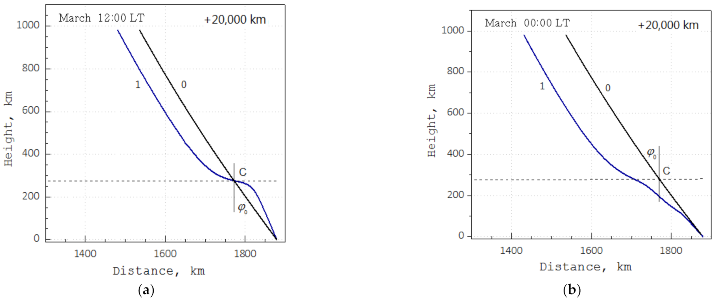
A modern trend in developing the mathematical representation of the upper atmosphere’s ionized part consists in modeling its high-latitude region. The polar ionosphere has a significantly more complicated structure than at middle latitudes. In particular, it is characterized by such large-scale plasma inhomogeneity as the auroral oval and the main ionospheric trough (MIT). The position of MIT and its geometrical parameters depend on the heliogeophysical activity level and the local time of the day. 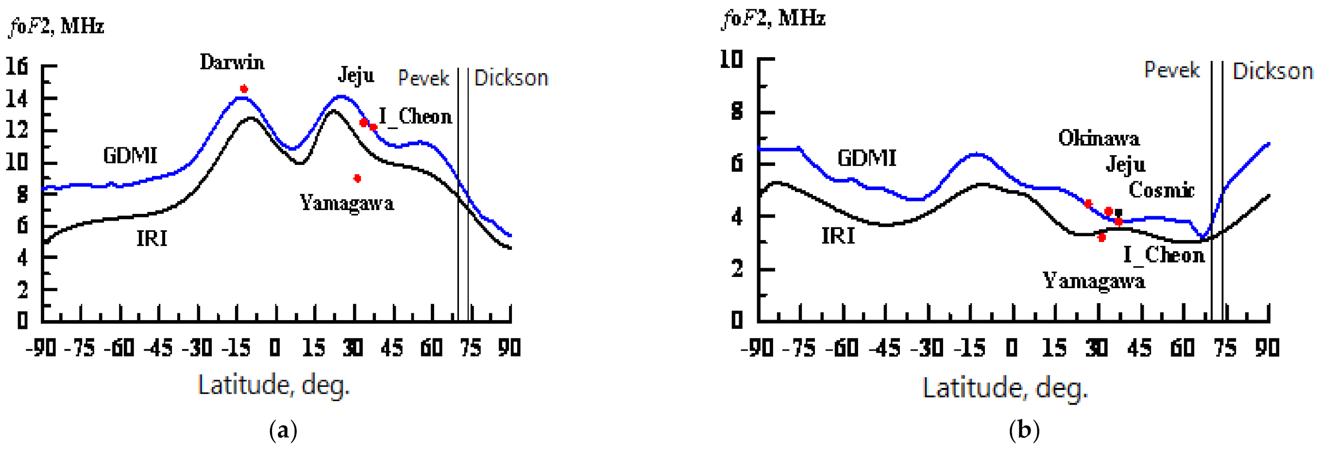For the first time, the presence of a trough in the electron density in the auroral region was shown experimentally by data from the Alouette satellite [15]. A typical example of foF2 longitudinal section for quiet geomagnetic conditions (Kp ~0) in the day and night times is shown in the plots of Figure 1, obtained from the median (monthly average) model IRI and its proposed development, the dynamic global model for the F2 layer (GDMI), taking into account the geomagnetic activity during the current and two previous days in the form of 3-h Kp-indices and current solar radiation in the form of radio flux (generalized index F10.7) [13]. Correspondently, the updated model pretends to be more accurate in an application to the daily time interval, including the polar areas. It can be seen that the dynamic model reflects in more detail the structure of the ionosphere at high latitudes. In particular, it describes the position of the main ionospheric trough, obtained analytically in [13]. With the growth of geomagnetic activity, MIT shifts to the equator. In addition to the main ionospheric trough, although not so regularly, a considerably weaker high latitude trough (HLT) is sometimes observed in satellite data [11].

The statistical (empirical) modeling is based on large arrays of experimental data about the spatial distribution of ionospheric parameters, covering various levels of solar and geomagnetic activity, which are rather difficult to collect in the conditions of the desert Arctic region. One of the possible ways to expand the experimental data is the multifrequency radio scanning of the ionosphere from geostationary or high-elliptical orbit (HEO) satellites [16]. The energy aspects of the high-orbit remote radio sensing problem and the peculiarities of its implementation in the geostationary mode were considered in [17].

In this paper, this method of basic radio and geophysical aspects are discussed as applied to the Arctic region, assuming radiation from having a highly elongated orbit satellite with an apogee in the vicinity of the Geographic North Pole.

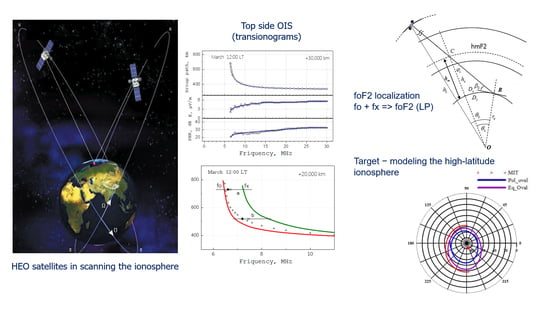
2. Multifrequency Radio Probing through the Ionosphere

This method consists of radio probing the ionosphere at frequencies, a typical characteristic of its plasma density, lying in the radio transparency range. With the separation of radio transmitting and receiving devices, their synchronization must be performed when scanning the operating frequency varying from 2 to 20 MHz. Thus, a system of one onboard transmitting module and independent ground-based receivers, synchronized with the emitter, becomes a diagnostic tool for the ionized medium. By analogy with VIS, the ionospheric information is taken from the registration of frequency-dependent group path of the radio signal, passing through the ionosphere, to the receiving point, assuming that the satellite spatial position is known (Figure 2).

The function describing the dependence of the group path versus the frequency, P’(f), of the ionogram of radio translucence (radio probing through), or transionogram, can be an object even simpler than the classical ionograms of VIS or oblique incidence sounding (OIS). This circumstance allows us to hope the automation of the process of its structure recognizing, interpretation, and processing, as it is a regular procedure in the VIS case. In this method, by analogy with the critical frequency foF2 in VIS or the maximum usable frequency (MUF) in OIS, the key point of the transionogram is the cut-off frequency, fc, equal to the lowest frequency that passes through the ionosphere by some propagation path, for instance, in the case of the F2 layer, by the 1F2 mode. As shown below, for the basic propagation mode, 1F2 (the shortest direct path from the satellite to the receiving point), this integral parameter can be related to the foF2 value at the intersection of the main ionospheric maximum with the line of sight to the satellite (sub-ionospheric point). Thus, there might be a potential opportunity for measuring the plasma frequency in the F2 layer peak.

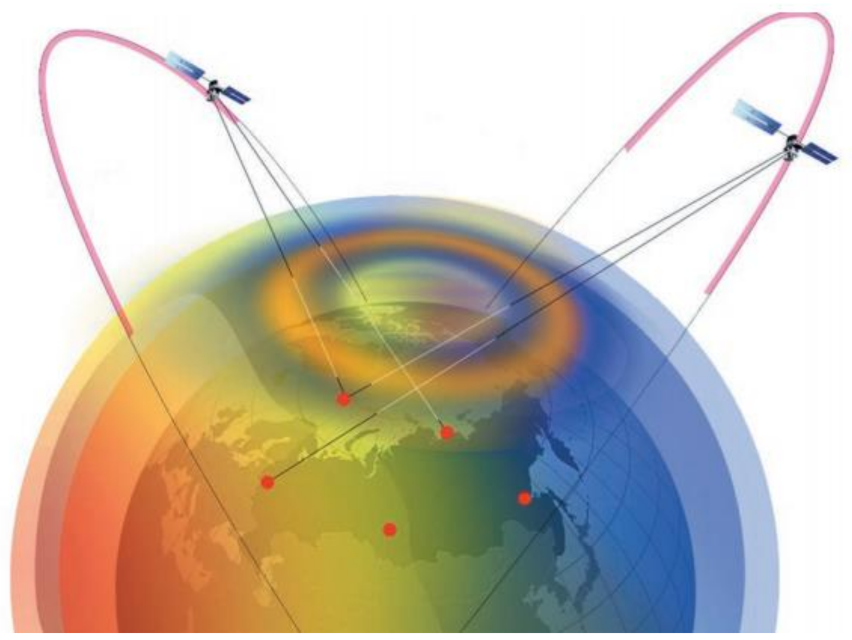
It is assumed this method can be implemented by mounting a wideband transmitter module on a highly elliptical spacecraft for hydro-meteorological monitoring of the Earth’s surface with an apogee over the Arctic zone, as shown in Figure 2. For the satellite with a 12-h synchronous orbital period, a working section of the orbit is 6–7 h, with an apogee altitude of 35,000–40,000 km. In the frames of the Russian Arctic-M program, the first such spacecraft for environmental monitoring in the Arctic zone was launched on 28 February 2021.

3. Mathematical Modeling

Similar to any other type of remote sensing of the ionospheric plasma, this technology of radio probing through the ionosphere with frequency scanning has the radio-physical and geophysical aspects of its application, mathematically related to the solutions for corresponding direct and inverse problem of radio wave propagation in the ionized medium. The technology’s radio-physical part consists in synthesizing the experimentally measured objects basing on the passage of radio waves in an inhomogeneous ionospheric plasma and extracting the signals from the background electromagnetic noises. The geophysical part is to reconstruct local values of the accessible ionospheric parameters by solving the corresponding inverse problem of radio sounding. In the method of multifrequency radio translucence, this object is a transionogram, and the estimated ionospheric parameter is the plasma frequency value at the maximum of the F2 layer. By analogy with the radio translucence method in GPS-TEC measurements, we consider the sub-ionospheric point as a localization point, where the optical line to the satellite intersects the level of the F2 layer maximum.

The energy problem, i.e., ensuring a sufficient level of the wave intensity for the received probing signals, is a decisive factor in the reliability and quality of transionograms in this method. We considered it in the frameworks of an idealized numerical experiment with a satellite located: (a) above the North Pole, and (b) close to Iceland (70°, 0°) with the heights of 10,000, 20,000, and 30,000 km. The reception of the probing signal was carried out in Dickson (73°N, 80°E). The global geomagnetic field was set in dipole approximation, with geomagnetic and Geographic North Poles coinciding. Two considered radio paths were oriented as follows: the first in the magnetic meridian plane (meridional direction) and the second in the latitudinal direction. So, we cover two limiting cases of wave propagation: (a) predominantly quasi-longitudinal and (b) close to the quasi-transversal approximation [18,19]. The paths’ length along the Earth’s surface are ~1900 and ~2600 km, respectively.

The modeling experiment technology is based on the geometric optics approximation in the point-to-point problem of radio waves propagation via the ionosphere, and a complex refractive index presentation [18,19] in the form of real and imaginary components was taken. The real part determines spatial divergence of the scalar wave field; the much smaller imaginary one determines the absorption of the wave energy by the medium plasma through the electron elastic collisions with ions and molecules of the atmospheric gases. For the field amplitude of a single mode, the solution of the transport equation has the form [20]:

$$A(\overrightarrow{r})\hspace{0.17em}=\hspace{0.17em}\frac{A_0^0}{\sqrt{J}}\sqrt{G_t{G}_r}\exp \left\{-k_0{\displaystyle \underset{L}{\int }\chi ds}\right\},$$

(1)

where is $A_0^0$ the initial value of the amplitude on a certain surface, empirically determined in millivolts per meter at a distance of 1 km for an isotropic antenna, with the radiation power in kW, $A_0^0=245\sqrt{P_t}$ [21]; $J=\hspace{0.17em}\frac{\mu da}{{\mu }_{0}d{a}_0}$ is the beam tube divergence (evolution of the beam cross-section along the ray trajectory); $G_t$, $G_r$ are the antenna gains; $k_0 = 2\pi /\lambda$ is the wave number; $\lambda$ is the wavelength; $\chi = -{\left.\frac{Z}{2\mu }\frac{\partial n^2}{\partial (Z)}\right|}_{Z=0}$ is the linear absorption coefficient; $X={\omega }_N^2/{\omega }^2$, $Y={\omega }_H/\omega$, $Z={\nu }_e/\omega$, ${\omega }_N$ is the plasma (cyclic) frequency, ${\omega }_H$ is the gyrofrequency, ${\nu }_e$ is the effective electron collision frequency with molecules and ions of the atmospheric gases; $L$ is the ray trajectory, connecting the terminal points of the radio path (propagation mode), determined by the canonical ray equations with the appropriate boundary conditions. The evolution of the beam tube is calculated using two orthogonal ray variations to this basic ray trajectory.

For the isotropic case ($Y=0$) and the refractive index in the Appleton–Hartree form [18,19], the attenuation coefficient has a simple form, convenient for the understanding of the physical principles and obtaining estimates in the radiation transfer problem [19]:

$${\mu }^2=1-X,\chi =XZ/2\mu ,$$

(2)

The group path, as well as the integral absorption, is determined by the integration along the basic ray path to a large extent, as in [22].

In this work, we analyze the principal possibility of getting localized estimates of the foF2 in the proposed method; therefore, we used averaged heliogeophysical conditions for the wavefield modeling. The calculations were carried out in the global median model of the ionosphere IRI (in its basic version), supplemented with the necessary additional ionospheric parameter, effective frequency of electron collisions [23], determining the wave energy absorption in the ionospheric plasma. The model selected time is the vernal equinox period (March); which has a middle level of solar activity, the sunspot number Rz = 50, and calm geomagnetic conditions. The analyzed results present two local times: noon, 12:00 LT (07:00 UT), and midnight, 00:00 LT (19:00 UT) in Dickson; at this point, there is a stationary ionospheric observatory.

The ray paths, along which the wave field transfers, for frequencies in the vicinity of the ionospheric radio transparency boundary on the meridional radio path, with the satellite localization height in 20,000 km, are shown in Figure 3 (curves 1). One can see that the greatest refraction effect by radio waves, passing through the medium, occurs in the vicinity of the main ionospheric maximum, where the real part of the refractive index becomes very small as the operating frequency approaches the radio transparency boundary. In this region, rapidly growing absorption of the wave energy also takes place, despite the relatively small value of effective electron collisions frequency (~10² s⁻¹) relation (2). For daytime and nighttime, the longitudinal gradients of electron density have opposite signs (Figure 1), defining the ray trajectories arrival at the receiving point. For the positive slope (electron density increases from the satellite to the receiving point), as in Figure 3a, the vertical arrival angle is slightly higher than the principal one (optical bearing to the satellite), and for the negative one, as in Figure 3b, vice versa.

The calculation of the energy characteristics was carried out under the following parameters and conditions (fundamental solution): The standard emitted power is 1 kW in the bandwidth of 1 kHz, the isotropic antennas are in the radiation and reception. The spatial divergence was determined with an account of the electron density inhomogeneity, absorption in the ionosphere, through the electron collision frequency. The longest path of the radio waves is under conditions of very low collision frequency.

The divergence factor is decisive in the resulting wave field strength; it significantly exceeds the collisional losses in plasma. However, the resonant absorption in the vicinity of the F2 layer maximum for the frequencies close to the radio transparency boundary can already have a comparable value. For this reason, we cannot register the accurate cut-off frequency, it has an asymptotic character. Both antennas transmitting on the satellite and receiving on the Earth’s surface were assumed isotropic; in the case of the real antennas, especially at the receiving end of the radio path, they may provide a significant gain in the problem of the probing signal extracting from background electromagnetic noises. The signal-to-noise ratio (SNR) was calculated as $SNR= 20\lg E_S/E_N$, where $E_S$ is the wave field strength of the probing signal, and $E_N$ is the root-mean-square field strength of the electromagnetic noise, which is determined in a given bandwidth [21] based on the global empirical EM noises model. A characteristic of the Arctic region is in a low level of anthropogenic noise, and as a rule it can be neglected. As a result, for example, at the frequency of 10 MHz for the meridional radio path with the transmitter height in 30,000 km – $E_S$~ 4.7 μV/m, the RMS value of the background noise in the 1 kHz bandwidth – $E_N$~ 0.25 μV/m, and accordingly SNR ~ 25 dB.

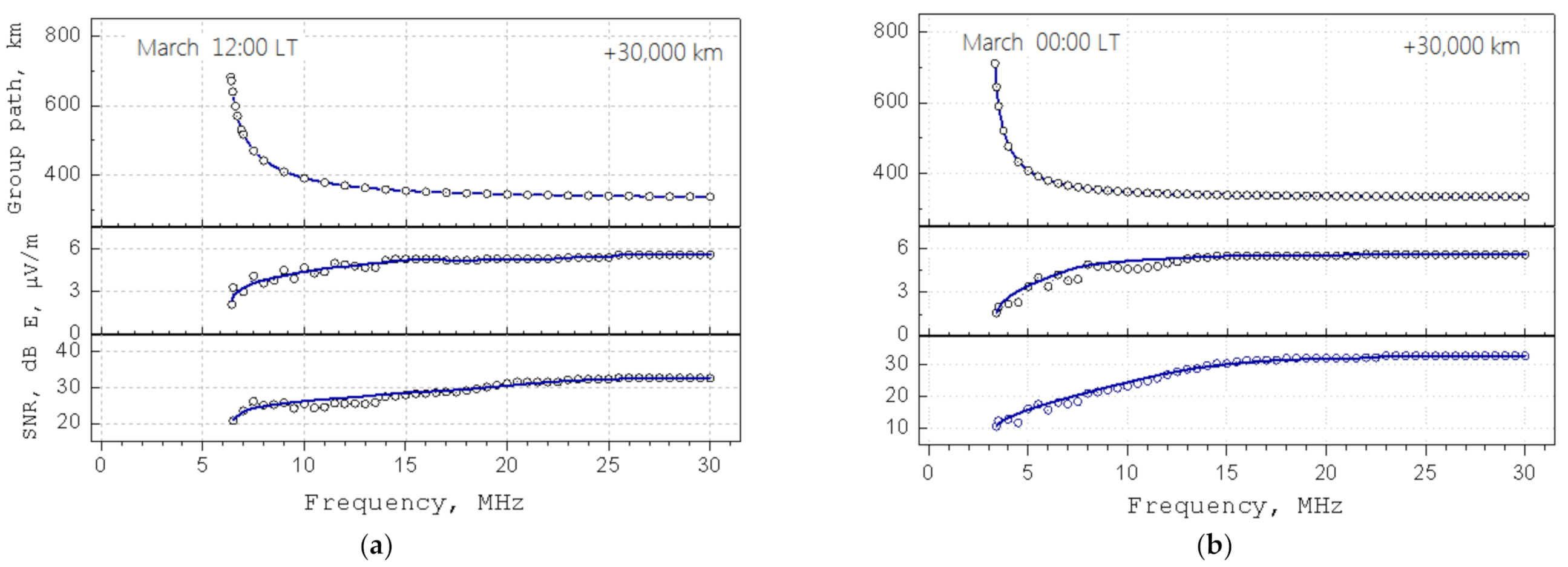
Figure 4 illustrates the general data, including the synthesized transionograms with the SNR and wave field strength obtained in the isotropic approximation of radio wave propagation with the refractive index and absorption (2). Figure 4a illustrates the data for local noontime, and Figure 4b—for local midnight. One can see that at frequencies in the close vicinity of the cut-off frequency, both the wave field strength and SNR sharply decrease. Moreover, for midnight the SNR is even less than for noontime due to a general pattern; with decreasing frequency, the level of electromagnetic noise increases together with the increasing wave energy absorption by the medium [21]. In addition, the nighttime ionosphere is characterized by higher values for both the maximum height (Figure 3) and the half-thickness of the F2 layer resulting in an increase in the passable path under conditions of the low refractive index. It should be noted that there are visible fluctuations in the wave field strength and in the SNR, which is apparently associated with anti-waveguide propagation along the maximum of the F2 layer. This process is characterized: (a) by a large divergence of the radio waves and (b) by high sensitivity to electron density irregularities (it may also be caused by some mathematical inaccuracy in the medium representation), leading to an appearance of the ray tube instability. Limiting the values of the field strength in both cases are ~6 μV/m, and the SNR is ~30 dB.

In practical realization of radio sensing methods in ionospheric research, the used frequency band is significantly wider than 1 kHz. For instance, a simple classical impulse with ~100 μs has a bandwidth (BW) ~10 kHz. Broadening BW leads to strengthening the background noise level, so for the frequency 10 MHz and 10 kHz BW, its RMS field strength increases to ~0.77 μV/m, and accordingly, SNR becomes ~15 dB, i.e., drops down significantly. Such a signal will already be close to the noise level near the cut-off frequency, especially for local midnight conditions (Figure 4b). In addition, the emission of pulsed signals of relatively high power can create problems in electromagnetic compatibility with other measuring and control equipment on the satellite board. An alternative approach is to use structured signals, now widely applied in radio sensing the ionosphere and radio communications via the ionosphere. However, in the highly elliptical spacecraft case, it is difficult to count on the phase-code-manipulated PCM signal consisting of the basis of modern ionosondes, such as the DPS-4 type [24] and some others, since its application requires an extended receiver bandwidth of up to 30 kHz. The gain due to the increased signal base is ~13–15 dB [24,25]. In addition, an inevitable influence of a chaotization and dispersive broadening of the signal elements (chips) during propagation over long distances in a dispersive medium on the correctness of the signal assembly at a receiving point is poorly studied. This effect, apparently, is noticeable in the OIS data obtained by this type of ionosonde [26].

At present, in the practice of ionospheric radio sensing, including experimental studies of probing waves scattering on small-scale irregularities, artificially generated by powerful radio waves, a proven tool is the usage of a frequency-modulated continuous-wave FMCW signal (chirp signal) [27,28,29]. Together with the high resolution, the chirp-signal technique requires a longer temporal interval in carrying out the sounding session. For instance, at the standard chirp speed of 100 kHz/s, it increases up to 3–4 min. In the case of the HEO satellite, the required frequency operating range is 2–20 MHz, and, accordingly, the session time will be equal to 3 min. Taking into account that the spacecraft position in the working area changes very little during this time scale, such an extension is not unacceptable. The actual increase in SNR, using FMCW signal technology, compared with a simple pulse one, can be up to ~30 dB [27], and this estimation was confirmed by the practice of radio-physical research of the ionosphere. Thus, the standard power of transmitting part ground-based VIS equipment works with: a simple classical pulse of ~10 kW, the PCM signal of 100–500 W, and 10–100 W in the FMCW case. Decreasing the radiation power to a level acceptable in the spacecraft conditions to 100 W (with several discrete levels from 10 to 100 W) lowers the SNR by 10 dB. At the same time, even reducing the benefit by order of magnitude to 20 dB (BW increases at the stage of the FMCW signal spectral processing), one can expect an increase in the SNR by 10 dB, which already allows us to hope for successful extraction of the signal from noises. Further ascending in receiving conditions is possible only due to an improvement of the receiving antenna gain. So, for example, for acceptable stationary observatory conditions, the phased array antenna (PAA) consisting of the four horizontal orthogonal wideband dipoles, the gain can be up to 10–12 dB. An application of orthogonal magnetic antennas is an equipment in the VIS research on DPS-4 ionosonde [24], which can provide a gain of ~3–4 dB in the case of individual application; overall lower EM noises characterize them, so this may be sufficient, for example, for the mobile receiving units.

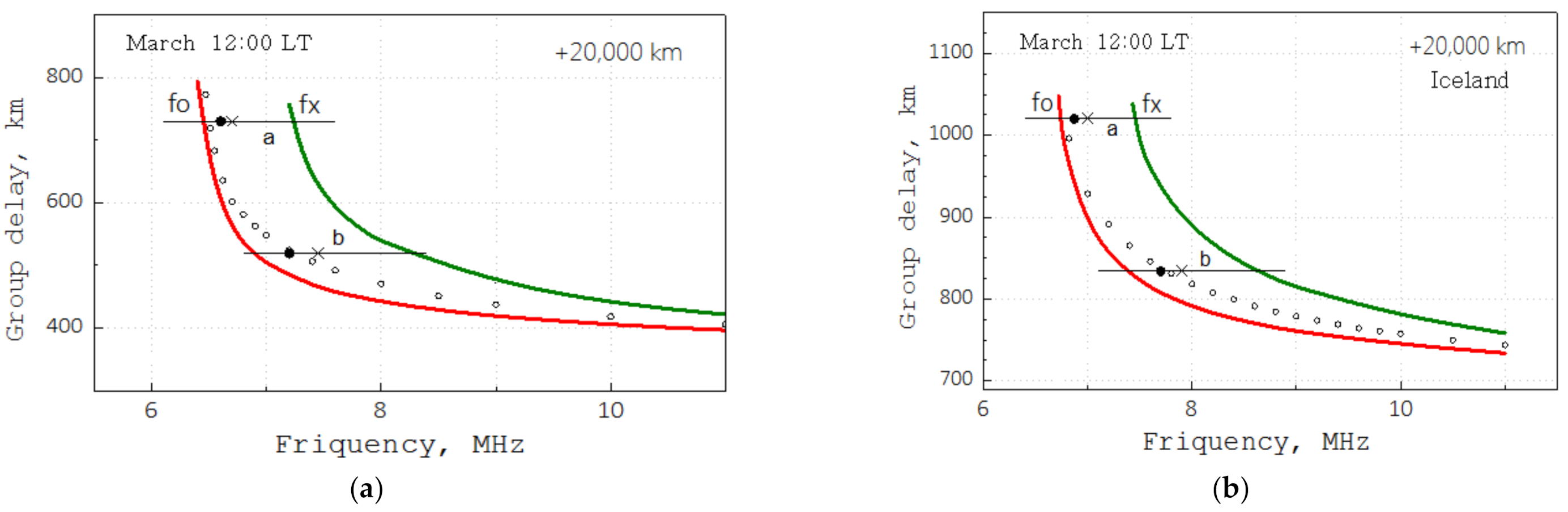
Due to the properties of magnetoactive plasma, the decisive factor complicating the transionogram structure is the geomagnetic field. Magnetoionic splitting appears in the form of ordinary (O-) and extraordinary (X-) components (in Figure 5, red color is the O-, and green is the X-component of the transionogram). The magnitude of the frequency split is slightly larger than, for example, at middle latitudes, which may equal ~0.8–1.0 MHz; this is associated with the enlarged value of the electron gyrofrequency and weakly depends on the radio path orientation to the geomagnetic field. For the radio path lying in the geomagnetic meridian plane, the case of quasi-longitudinal propagation of radio waves is almost realized, the ratio of the longitudinal and transversal components of the gyrofrequency at the sub-ionospheric point C (Figure 3) is about 3. For the latitudinal radio path, this ratio is ~1. However, as shown in Figure 2, the curvature of ray trajectories near the maximum of the F2 layer practically leads to a quasi-transverse type of propagation on both analyzed paths. It leads to a deformation of the O-branch in the transionogram so that its asymptotic become close. A similar picture takes place with the transionogram branches for the latitudinal radio paths (Figure 5).

Another factor that can lead to additional traces in a transionogram is the large-scale horizontal inhomogeneity of the ionosphere at high latitudes. Such modes may exist only in a narrow frequency range and have significantly lower energy than the main mode trace. So, in local noon time (Figure 3a), there is a certain probability of a combined mode appearance with a second jump caused by intermediate reflection from the Earth’s surface due to increasing the electron density in the longitudinal direction. In addition, under specific spatial configurations of the radio path, the ionospheric trough walls, for which the horizontal inhomogeneity (transverse gradient) is quite significant at nighttime (Figure 1), may form additional reflections. This can lead to duplicating tracks on the transionogram, similar to the propagation along the trough in terrestrial conditions.

4. Localization of the Critical Frequency Estimates

From physical considerations, it is clear that the determining factor in forming the cut-off frequency is the plasma frequency at the region of crossing the F2 layer peak by ray trajectories, and seen in Figure 3. The ray tube’s physical size, defining the spatial resolving ability, is determined by the radius of the first Fresnel zone ~$\sqrt{\lambda z}$, where $\lambda$ is the wavelength, and $z$ is the actual satellite height, reaching a value of ~50–70 km.

The actual location of this region on the Earth’s surface depends on the sub-satellite point position, the altitude of the satellite itself, and the longitudinal gradient of electron density. With the positive electron density gradient along the satellite-receiver arc, the typical case is shown in Figure 3a and a small or negative one in Figure 3b. 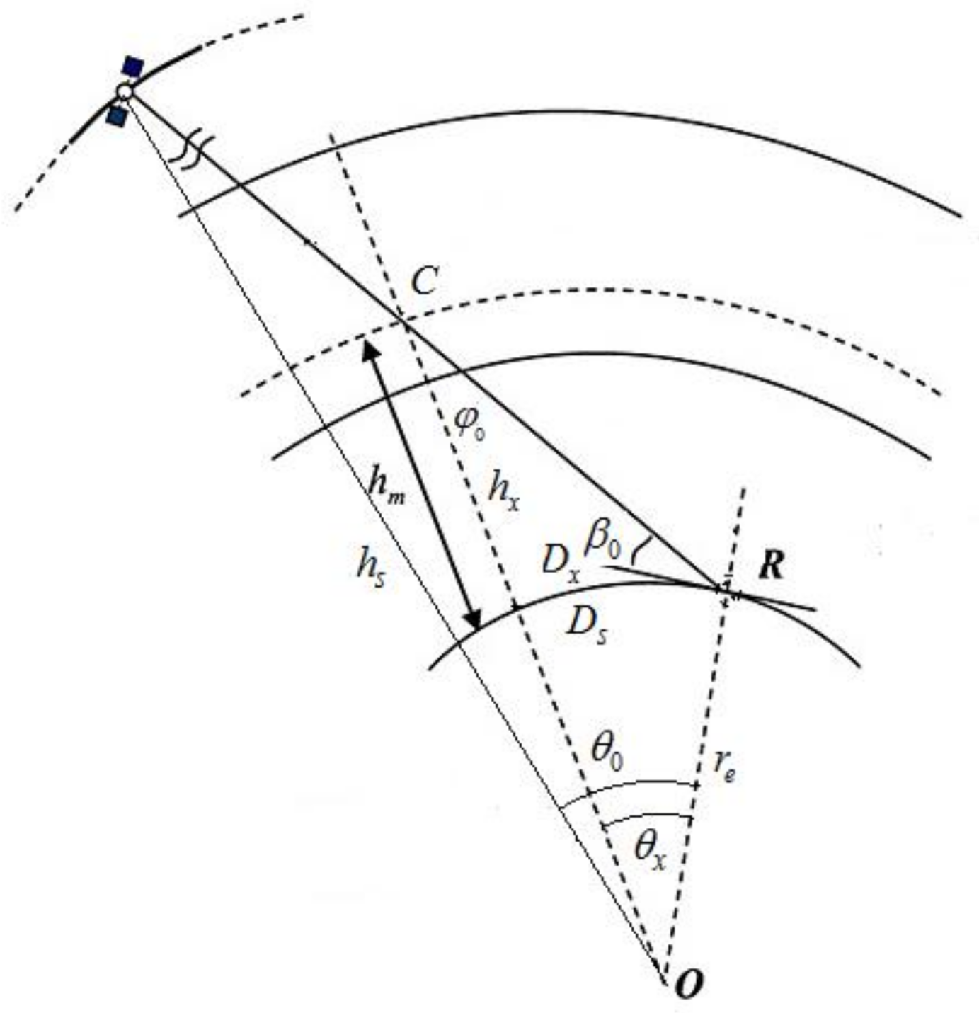In an actual situation, as a rule, it is difficult to account for the factor of longitudinal inhomogeneity, and it seems feasible to consider a simplification when the localization region is defined as the intersection point by a line-of-sight and the curve of the F2 layer ionospheric maximum, indicated as point C in Figure 3. Mathematically, this point with coordinates in the great circle plane $\left(D_x, h_x\right)$, $h_x$ being the height above the Earth’s surface and $D_x$ is the distance from the receiving end (Figure 6), which is determined by the equations:

$$\begin{array}{l}\left(r_e+h_x\right)\sin ({\theta }_x) - \cos {\beta }_0\sqrt{r_e^2 + {(r_e+h_x)}^2-2r_e(r_e+h_x)\cos {\theta }_x } = 0\\ h_x= h_{m}F2\left(D_x\right) .\end{array}$$

(3)

where ${\theta }_x=D_x/r_e$; ${\theta }_0=D_s/r_e$; $\left(D_s, h_s\right)$ is the satellite position in the two-dimensional coordinate system; $r_e$ is the Earth’s radius; $h_{m}F2\left(D\right)$ is the F2 layer maximum (taken from a model representation); and ${\beta }_0$ is the elevation angle of the line of sight on a satellite, defined as:

$$\cos {\beta }_0= \left(r_e+h_s\right)\sin {\theta }_0/\left(\sqrt{2r_e\left(r_e+h_s\right)\left(1-\cos {\theta }_0\right) +h_s^2}\right).$$

(4)

One can find a solution of the equations (3) numerically through the method of successive approximations. The initial value $h_x^0$ can be set equal to 300 km (both for day and night conditions), then $D_x^0$ can be obtained from the first equation, and the next approximation for the height $h_x^1$, from the second etc. Usually, three iterations are enough to obtain a solution $\left(D_x, h_x\right)$. Then it is possible to determine the geographic coordinates of the solution point, knowing the azimuth and the distance to the sub-satellite point from geographic coordinates of terminal points. The model critical frequency at the localization point is defined as $f_{o}F{2}_{\mathrm{mod}}= f_{o}F2\left(D_x\right)$. Functions $f_{o}F2\left(D\right)$ and $h_{m}F2\left(D\right)$ are model interpolation functions of the main ionospheric peak along the arc connecting the receiving and sub-satellite points.

In our case, as in the general situation of oblique radio waves propagation, the cut-off frequency is greater than the plasma frequency at the point where its trajectory is crossing the hmF2 level. For the isotropic one-dimensional media, this effect is expressed by the equivalence theorem [19]:

$$f_{obl}=f_v\cdot \sec {\phi }_0,$$

(5)

where $f_{obl}$ is the probing frequency, $f_v$ is the equivalent vertical reflection frequency, ${\phi }_0$ is the angle of ray trajectory intersection with the lower boundary of the ionosphere, determined by the angle of arrival. Based on the results obtained from the first oblique incidence experiments [29] some correction was introduced:

$$f_{obl}=k_{eff} f_v\cdot \sec {\phi }_0,$$

(6)

where $k_{eff}$ is the correction factor for sphericity, depending on the path length and lying in the range 1.0–1.2 [30]. At path lengths up to 300 km, the correction factor is close to 1.0. Assuming the localization point, the sub-ionospheric point C (Figure 3), we obtain:

$${\phi }_0=\pi /2- {\beta }_0-{\theta }_x,$$

(7)

As follows from the magneto-ionic theory [17] and is evident from Figure 5, the cut-off frequency of the ordinary component should be the lower boundary for its value in the isotropic approximation. Only in the limiting case of genuine transversal propagation, their values are equal. The following procedure can estimate the upper boundary based on a significant similarity of the transionogram traces—“isotropic”, O- and X-components (Figure 5). One can assume that there are the frequencies belonging for each branch, for which, under the condition of their group paths equality, the sounding radio waves pass approximately along the same ray trajectories. As shown above, the greatest influence on propagating radio waves causes the F2 layer maximum. So, supposing it defines the localization point, one can write down:

$${\mu }^2\left({\overrightarrow{p}}_o,f_o,{\overrightarrow{r}}_l\right) \approx {\mu }^2\left({\overrightarrow{p}}_x,f_x,{\overrightarrow{r}}_l\right) \approx {\mu }^2\left(\overrightarrow{p},f,{\overrightarrow{r}}_l\right),$$

(8)

where $\overrightarrow{p}$,${\overrightarrow{p}}_o$,${\overrightarrow{p}}_x$ are unit wave vectors of characteristic waves, ${\overrightarrow{r}}_l$ is the localization point. For the passing through modes, the parameter $X=f_N^2({\overrightarrow{r}}_l)/f_{}^2 <\hspace{0.33em}1$, where $f_N({\overrightarrow{r}}_l)$ is the plasma frequency, and $f$ is the operating frequency. Expanding the real part of the refractive index in the Appleton–Hartree form [18,19] in powers $X$ up to the first order, we obtain:

$${\mu }^2\left(\overrightarrow{k},\omega ,\overrightarrow{r}\right)\simeq {\left.{\mu }^2\left(\overrightarrow{k},\omega ,\overrightarrow{r}\right)\right|}_{X=0}+{\left.\frac{\partial {\mu }^2\left(\overrightarrow{k},\omega ,\overrightarrow{r}\right)}{\partial X}\right|}_{X=0}\cdot X= 1-\frac{f_N^2}{f_{0,x}^2-\frac{f_T^2}{2}\pm {\left(\frac{f_T^4}{4}+f_{0,x}^2{f}_L^2\right)}^{1/2}}$$

(9)

where $\overrightarrow{k}$ is the wave vector, $f_L$ and $f_T$ are the longitudinal and transverse components of the electron gyrofrequency to the direction of the wave vector, from which it follows that under fulfilling the following relationship between the frequencies for isotropic and magneto-ionic components:

$$f^2=f_{0,x}^2-\frac{f_T^2}{2}\pm {\left(\frac{f_T^4}{4}+f_{0,x}^2{f}_L^2\right)}^{1/2},$$

(10)

the refractive index corresponds to the form typical for the case of isotropic propagation mode.

The relations (6) with the gyrofrequency components in the sub-ionospheric point (Figure 3, point C) perform well enough in the situation when the curvature of the ray trajectories is insignificant (Figure 5b). Thus, in the case of quasi-longitudinal propagation (Figure 5a,b): for the O-component the pair meanings $f_o$ and $f_i$ (isotropic) in (6) are [6.9;7.4], for the X-component, respectively [8.2;7.6]. The genuine frequency value for the isotropic branch in this cross-section is 7.3, i.e., the estimates from the magneto-ionic points of the transionogram are close enough to it. The averaged “isotropic” frequencies, with equal weights from both “experimental” branches near the cut-off frequency (Figure 5, cross-sections a) and at some distance from it (Figure 5b), are plotted by crosses. It can be seen that their values indeed are the upper limits for the virtual points of “isotropic” transionograms. The arithmetic mean of the upper and lower boundaries (marked by solid points) for the cross-sections (a) in Figure 5 was used as a frequency value $f_{obl}$ in (4), then $f_v$ is an estimation for the critical frequency foF2.

Such an approach improves the stability of the problem as a whole, and the results of foF2 estimation in the meridional sounding plane are summarized in

Table 1. Inaccuracy in the estimation of foF2, 12:00 LT.

Height,	fo,	fx,	foF2(m),	foF2(c),
km	MHz	MHz	MHz	MHz
10,000	6.4	7.2	6.1	6.0
20,000	6.4	7.2	6.2	6.1
30,000	6.3	7.1	6.2	6.1

and

Table 2. Inaccuracy in the estimation of foF2, 00:00 LT.

Height,	fo,	fx,	foF2(m),	foF2(c),
km	MHz	MHz	MHz	MHz
10,000	3.5	4.2	3.1	3.2
20,000	3.4	4.1	3.1	3.2
30,000	3.3	4.1	3.1	3.2

. Here fo, fx are the taken estimates for the cut-off frequencies from magnetoionic components (Figure 5), foF2(m)-model (seen as a reference), and foF2(c)-calculated (according to described above procedure) critical frequencies in the sub-ionospheric point. For noon, the calculated values for both types of radio paths are somewhat smaller than the true ones and slightly larger for midnight. Such a peculiarity in the foF2 estimation inaccuracy seems to be related to the angle value by direct line on the satellite crossing hmF2, ${\phi }_0$ (in Figure 6). For noon conditions, its actual meaning is less than the basic angle due to a larger elevation angle ${\beta }_0$ (6) ($f_{obl}\cos {\phi }_0$ will accordingly be larger); the situation is the opposite for half-night (Figure 3b). This circumstance is a consequence of simplifying the problem by replacing a complex trajectory with the asymptotic representation based on the line-of-sight approximation. Possible improvements, including the hmF2 estimation aspect, may be achieved based on the existence of analytical solutions for ray trajectories in simplified cases of the ionospheric layer models, such as, for instance, the quasi-parabolic approximation.

The overall estimated RMS deviation of critical frequency obtained from the simulation results (12 satellite-receiver point combinations) does not exceed 0.2 MHz, being slightly larger than the standard mathematical error for VIS ionosonde (~0.1 MHz) but significantly smaller than the error in the method using TEC measurements (~0.4 MHz) [31]. This approach of obtaining the localized estimation of the plasma frequency in the F2 layer peak from the measured cut-off frequencies seems universal independently from an orientation of the radio path plane. It also can be applied to radio sensing data from geostationary satellites in the middle and low latitudes.

5. Discussion

The results of the numerical modeling of the radio-physical and geophysical aspects of the proposed method for a diagnostics of the ionosphere from high apogee spacecraft aimed to an environment control over the Arctic region provides information for the following conclusions:

(a) The technical implementation of the method is quite possible founded on an application of the approved version of structured signals with acceptable emission power in satellite compatibility conditions;

(b) Registration of the cut-off frequencies on the magnetoionic components of the transionogram allows one to estimate the local (in the sub-ionosphere point) value of the fundamental ionospheric parameter, the plasma frequency in the F2 layer maximum.

The possibility of the physical implementation of the radio translucence method in the ionospheric plasma frequency range between high-orbit satellites and Earth’s surface can be supported by experimental data. The method peculiarity is a long satellite-ground point radio path, but it lies in rarefied plasma with a low electron collision frequency, which to a certain extent corresponds to the radio waves passage.

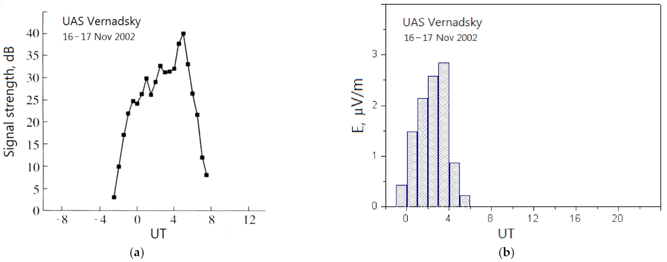
As an analog in terrestrial conditions, one can consider the experimental results of registering referenced frequencies from the exact time in Moscow, RWM at the Ukrainian Antarctic station “Academician Vernadsky” (65°15′S, 64°16′W) in 2002–2005; in particular, a propagation of 4996 kHz radio waves [32]. The shortest distance between the terminal points is ~16,000 km; the emitted power is 5 kW. The working frequency of 5 MHz is low enough, resulting in the wave’s strong attenuation due to the absorption in the D and E layers during the hop-mode propagation. For this reason, there is a time interval of quasi-antipodal passaging in the diurnal period (Figure 7a), the signal was registered only under almost entirely nocturnal conditions along the radio path [33]. The calculated field strength (Figure 7b) is comparable with the values characteristic for the radiation from a high-orbital satellite in basic solution (Figure 4). A similar situation takes place with the signal-to-noise ratio, in the satellite case; it is ~25 dB, which is comparable with the experimental data on the measured signal intensity (Figure 7a).

A realization of experimental research with a transmitter on the high-orbital satellite over the Arctic region may have an extended radio-physical aspect concerning the probing radio waves attenuation when propagating via ionospheric plasma. It is known that, in contrast to the electron density plasma models, the models for the effective electron collisions frequency are much less reliable and justified, and the Banks formula [23] used in this work are not the only option for representing this property of the ionosphere; neither is the introduction of alternative representations of the refractive index (Sen Wyller formulation) when calculating radio wave absorption in the ionosphere [34]. Obtaining the radio-translucence data in a wide frequency range practically in the static experiment with well-known parameters of radiation, antennas, and propagation conditions monochromatic radio waves may significantly improve knowledge of the key ionospheric parameter.

6. Conclusions

Our mathematical simulation results and analysis of experimental data on super long radio paths show the real possibility of estimating the plasma frequency in the F2 layer peak of the ionosphere (sub-ionospheric point) according to a radio translucence of the Arctic ionosphere with the use of radiation with frequency sweeping from a highly elliptical spacecraft. According to the measurements of the cut-off frequencies from the transionograms, the expected potential mathematical accuracy of the method concedes to the most reliable data of vertical radio sounding of the ionosphere in the ground-based conditions, but in general, surpasses the technique using the measurements of the total electron content in the GPS technology. This method can be implemented by setting the specialized transmitting module on the satellites specified for hydro-meteorological control of the Earth’s surface with the apogee and working section of the orbit over the Arctic zone.