Abstract
Radar instruments have been widely used to measure snow water equivalent (SWE) and Interferometric Synthetic Aperture Radar is a promising approach for doing so from spaceborne platforms. Electromagnetic waves propagate through the snowpack at a velocity determined by its dielectric permittivity. Velocity estimates are a significant source of uncertainty in radar SWE retrievals, especially in wet snow. In dry snow, velocity can be calculated from relations between permittivity and snow density. However, wet snow velocity is a function of both snow density and liquid water content (LWC); the latter exhibits high spatiotemporal variability, there is no standard observation method, and it is not typically measured by automated stations. In this study, we used ground-penetrating radar (GPR), probed snow depths, and measured in situ vertically-averaged density to estimate SWE and bulk LWC for seven survey dates at Cameron Pass, Colorado (~3120 m) from April to June 2019. During this cooler than average season, median LWC for individual survey dates never exceeded 7 vol. %. However, in June, LWC values greater than 10 vol. % were observed in isolated areas where the ground and the base of the snowpack were saturated and therefore inhibited further meltwater output. LWC development was modulated by canopy cover and meltwater drainage was influenced by ground slope. We generated synthetic SWE retrievals that resemble the planned footprint of the NASA-ISRO L-band InSAR satellite (NISAR) from GPR using a dry snow density model. Synthetic SWE retrievals overestimated observed SWE by as much as 40% during the melt season due to the presence of LWC. Our findings emphasize the importance of considering LWC variability in order to fully realize the potential of future spaceborne radar missions for measuring SWE.
1. Introduction
At its seasonal maxima, snow covers more than 60% of the land surface in the Northern Hemisphere [1,2] and influences hydrologic, biologic, and climate systems in far-reaching ways [3,4,5,6,7]. Snowpacks in mountainous regions provide a critical water resource to over 1.2 billion people globally [5], but these regions are responding rapidly to climate change and are warming at faster rates than low-elevation temperate and equatorial regions [8,9]. Over the past half-century in the western USA, snow water equivalent (SWE), the amount of water stored in the snowpack, has declined by 15–30% and melt onset is occurring 2–3 weeks earlier [10,11,12,13,14]. This decline in SWE agrees with the observed decline in Northern Hemisphere snow-covered area during spring and summer months, but contrasts with the observed increase in snow-covered area during winter months [15]. Additionally, warming temperatures are projected to change the dominant precipitation phase that falls during traditionally snow-dominated months and drive the rain–snow transition zone higher in elevation (e.g., [16]). Collectively, these changes indicate a pronounced shift in the historic baseline for mountain snowpacks, but these changes are not well understood globally (e.g., [17]). Thus, improved monitoring at the global scale is required for informed water resource management decisions.
SWE is the defining variable of the snowpack that is used in runoff forecasting, water resource management, and drought predictions [18]. Numerous remote sensing approaches are used to measure SWE, but each approach has associated limitations and uncertainties, and no single approach has proven successful across the diverse range of snow environments and conditions that exist [19]. Passive microwave sensors are traditionally limited to shallow (SWE < 200 mm) snowpacks [19,20] and have increased uncertainty in complex topography given their large spatial footprint [21,22]. The GlobSnow product, a long-term hemisphere-scale dataset of snow parameters, masks out mountain regions for the passive microwave data, due to highly varying topography within the sensor footprint [23].
Airborne light detection and ranging (lidar) methods are capable of resolving fine-scale (<1 m) snow depth heterogeneity, but are currently limited to regional-scale studies [24,25]. Satellite-based lidar instruments (e.g., ICESat-2) show promise, but current repeat orbits (91 days) provide insufficient temporal resolution for monitoring SWE. Satellite-based photogrammetry methods [26,27,28] are increasingly being utilized, but coregistration in completely snow-covered landscapes remains a challenge, and thus are most suited to environments free of tree-cover [29,30]. Radar methods, including Interferometric Synthetic Aperture Radar (InSAR), are a viable means of estimating SWE [31] and snow depth [32], but there are uncertainties regarding radar performance in various environments, especially wet snow. Current radar approaches that use backscatter observations at C-, X-, and Ku-band to estimate SWE and depth are not applied during wet snow conditions due to the complexity in interpretation and limited penetration; however, changes in backscatter magnitude can be used to identify wet and dry snow from spaceborne radar (e.g., [33]). Data fusion methods are a promising path towards increasing the accuracy of SWE estimates (e.g., [34]), yet such methods inherently require multiple sources of data input, such as snow reanalysis products and in situ SWE observations, and therefore cannot operate in isolation. The global solution to SWE estimation will require a combination of multiple remote sensing approaches, in situ measurements, and models.
Radar transmissibility through snow is a function of snow grain size and wavelength of the radar frequency, where L-band (1–2 GHz; 15–30 cm wavelength) is highly transmissible [35], C-band (4–8 GHz; 3.75–7.5 cm wavelength) scatters with larger snow grains [36], and Ka-band (26.5–40 GHz; 0.75–1.11 cm wavelength) has limited penetration [37]. InSAR methods have been used to map snow cover extent in C-band and X-band (8–12 GHz; 3.75–2.5 cm wavelength; [38]), snow depth from airborne Ka-band [37], and snow depth in non-forested regions from Sentinel-1 C-band cross-polarization and co-polarization backscatter ratios [39]. Given the transmissibility of L-band radar in snow and the potential for mapping SWE through InSAR methods, recent NASA SnowEx campaigns have focused on evaluating NASA’s UAVSAR L-band (1.26 GHz) sensor for measuring changes in SWE. These campaigns consisted of: (1) a ~2 week long SnowEx 2017 campaign at Grand Mesa, CO, (2) a weekly to bi-weekly SnowEx 2020 Time Series campaign at thirteen sites in the western USA, and (3) a weekly SnowEx 2021 Time Series campaign at six sites in the western USA. Minimal changes in SWE during the SnowEx 2017 campaign precluded a thorough assessment of InSAR phase-change vs. SWE-change [40,41]. The SnowEx 2020 and 2021 Time Series campaigns, with a longer duration and a greater number of study sites in diverse snow climates, provide the opportunity for a more thorough assessment of this phase-change approach. This assessment is pressing given the NASA-ISRO L-band InSAR satellite mission (NISAR) is scheduled for launch in early 2023. However, a principal uncertainty in L-band radar SWE remote sensing is the variability in radar velocity introduced by wet snow conditions.
Radar velocity depends on the dielectric permittivity of the snowpack and is sensitive to snow properties. Permittivity in dry snow, a mixture of air and ice, is primarily a function of snow density [42], but in wet snow, permittivity is a function of both density and liquid water content (LWC; [43]). GPR is an established method for measuring snow depth and SWE (e.g., [29,44,45]), making it an ideal instrument to evaluate L-band velocity uncertainties in snow. The radar physics in snow is similar between GPR and InSAR, although key differences exist between the specific methods. GPR produces geolocated radargrams where the snow–ground interface must be identified, while InSAR is a change detection approach, requiring repeat overpasses to measure changes in radar phase that occur from one acquisition to the next [31,46] and are related to changes in the travel time through the snowpack.
LWC is primarily generated through surface melt when the net energy balance is positive (e.g., [47]), although rain-on-snow events can also be a significant source (e.g., [48]). In the spring, the snowpack ripens to 0 °C as the positive energy balance in the upper strata produces meltwater at the surface that percolates through the snowpack, where it either refreezes or is stored. This process warms the temperature of lower strata and lowers the cold content of the snowpack [49]. After ripening, meltwater production rates that exceed snowpack porosity, result in water that can move laterally (e.g., [50,51]) or vertically, and are eventually output at the base of the snowpack [52,53,54]. During this generalized sequence, and especially during the transition from dry to ripe snow, there is high temporal and spatial variability in LWC, with complex relations between LWC and slope, aspect, elevation, and canopy cover (e.g., [52,55,56]).
Temporally, LWC has both a diurnal and seasonal response to variations in the net energy balance [43,54,57]. During the ripening phase of the melt season, LWC diurnal change is limited to 0–1 vol. % [54]. As the melt season progresses, the wetting front moves through the snowpack [58]. At the end of the melt season, LWC diurnal change can be 3–4 vol. % [54]. At the hillslope to plot scale, preferential flowpaths develop (e.g., [59,60]) to transport meltwater along strata or via vertical piping. This results in highly heterogenous patterns of LWC and meltwater delivery to the base of the snowpack (e.g., [60,61]). Preferential flowpaths can also develop along the snow–ground interface, causing water to pool where local surface slopes flatten (e.g., [50,60]).
Unlike snow density, LWC is not typically measured at automated stations (e.g., SNOTEL stations), so most LWC observations are collected in snowpits, using either capacitive sensors that measure the dielectric permittivity of the snow (e.g., [53,62,63]) or calorimetry methods (e.g., [64]). However, snowpits disturb the snowpack stratigraphy and likely alter LWC patterns, thus new methods based on GPS signal attenuation (e.g., [35]), upward looking GPR (e.g., [43,58]), and the combination of GNSS and upward looking GPR (e.g., [54]) provide non-destructive observations but have not been deployed operationally. In our study, LWC is measured non-destructively along transects using a combination of distributed independent snow depth measurements and GPR travel times, an approach implemented by Webb et al. (2018c).
Radar velocity in snow, as defined by a three-phase (i.e., ice, water, and air) mixing formula ([65]; Figure 1), is more sensitive to changes in LWC than changes in density. Therefore, the presence and spatiotemporal variability of LWC in seasonal snowpacks is a greater source of uncertainty for radar velocity estimates than snow density assumptions [54,57,66]. Consider a scenario (Figure 1b) where a radar signal’s one-way travel time through a snowpack of 400 kg m–3 density was 5 ns, but the presence/magnitude of LWC is unknown and assumed to be 0 vol. %. In this case, if this snowpack had 7 vol. % LWC, SWE would be overestimated by 40%. In comparison, if the density of this snowpack was 250 kg m–3, SWE would be overestimated by 25%. LWC influences the accuracy of radar SWE retrievals so substantially because the relative permittivity of water is 35–60-fold greater than the relative permittivity of seasonal snow.
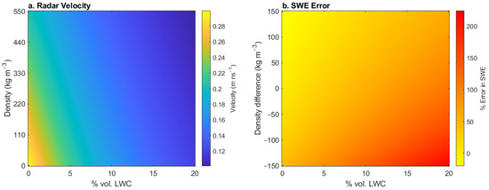
Figure 1.
(a) Radar velocity in snow as a function of snow density and LWC. (b) SWE error calculated as the percent difference between an “assumed” SWE and a “true” SWE for a radar signal with a travel time of 5 ns in snow. “Assumed” SWE was calculated using 400 kg m−3 and 0% vol. LWC. “True” SWE was calculated using densities from 250 to 550 kg m−3 and LWC from 0 to 20% vol. These figures use Equation (3) to relate permittivity, density, and LWC.
Here, we quantify the uncertainties associated with radar SWE retrievals, at a footprint approximating that of NISAR, by examining (1) the spatiotemporal variability of LWC at 9 m intervals along three transects that total ~850 m, (2) the influence of terrain and canopy cover on LWC in a continental seasonal snowpack, and (3) the error in radar SWE retrievals when LWC is unknown and assumed to be zero. To address these objectives, we used a Sensors and Software PulseEkko Pro 1 GHz surface-coupled common-offset GPR, in situ snow measurements, terrestrial lidar, and nearby automated meteorological and stream gauge stations.
2. Study Area
Cameron Pass (3120 m) is located between the Medicine Bow and Never Summer Mountain Ranges of north-central Colorado and is a headwater region for the Cache la Poudre River Basin. The study area is within the subarctic climate (Dfc) of the Köppen-Geiger Climate Classification [67] and is forested with Engleman spruce (Picea engelmanii), subalpine fir (Abies lasiocarpa), lodgepole pine (Pinus contorta), and Aspen (Populus tremuloides), with interspersed meadows (Figure 2; [68]). Field surveys were completed along three transects, each representing a unique set of terrain parameters and canopy densities. The North Transect has an elevation range of 3120–3126 m, 0–5° slopes, NE aspect, and 20–70% canopy cover. The Meadow Transect has an elevation range of 3121–3126 m, flat aspect and no canopy cover, but is shaded until mid-morning (~09:00 MDT in June) by the north ridge of Iron Mountain (3670 m). A tributary to the Michigan River, a ~1 m wide meandering stream, parallels the Meadow Transect and intersects it twice. The South Transect has an elevation range of 3111–3123 m, 3–14° slopes, W–S aspect, and canopy that varies from 0% in the southernmost portion of the transect to ~70% in the western portion of the transect.
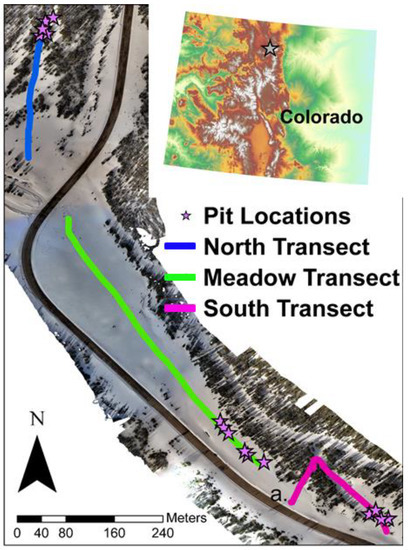
Figure 2.
Cameron Pass field site. The three transects are shown by the colored lines and snowpit locations are marked by stars. The inset shows the location for Cameron Pass within Colorado, USA. Orthomosaic derived from sUAS survey in March 2020. DEM in inset obtained from the Shuttle Radar Topography Mission (https://srtm.csi.cgiar.org/, accessed on 14 May 2019). Marker a. denotes the western terminus of the South Transect.
3. Methods
3.1. Nearby Automated Stations
We calculated median SWE, snow depth, air temperature, and length of melt season (defined as the temporal interval between peak SWE and snow off) for April-June using the 1978–2018 daily records from the Joe Wright SNOTEL station (https://wcc.sc.egov.usda.gov/nwcc/site?sitenum=551, accessed 2 April 2021), located 1.4 km to the northeast of our study site at 3084 m elevation, and compared them with the 2019 daily records. We estimated hourly snow depth loss during select survey dates using a least-squares regression. We calculated positive degree days (PDD; [69]) from hourly SNOTEL air temperatures as the scaled cumulative sum of positive hourly temperatures, as:
where is the time in hours after 00:00 MDT and is a positive temperature (°C) at time .
We used streamflow data to assess meltwater output from the local watershed, specifically Joe Wright Creek (https://waterdata.usgs.gov/nwis/uv?site_no=06746095, accessed on 9 April 2020) ~2.4 km to the northeast of the field site. This watershed receives trans-basin inflow from the Michigan Ditch (https://dwr.state.co.us/Tools/Stations/MICDCPCO?params=DISCHRG, accessed on 9 April 2020). The Michigan Ditch discharge was subtracted from Joe Wright Creek discharge to remove this trans-basin water input. The discharge was converted to a daily depth of water by dividing discharge by the basin area (8.13 km2).
3.2. Observational Period
At Joe Wright SNOTEL station, median peak SWE for 1978–2018 occurs on 5 May (standard deviation = ±27 days) and the median snow off date is 17 June (standard deviation = ±13 days). Field surveys captured LWC variability throughout the 2019 melt season, consisting of a pre-melt dry snow survey on 5 April, an initial melt season survey on 25 April, and five middle to late season surveys conducted from 17 May to 19 June (Table 1).

Table 1.
Observations performed for each survey date. Depth transects were collected once per survey date and were acquired as either a complete transect or a partial transect. GPR transects were performed up to three times per survey date.
3.3. Field Methods
For each survey date, we sampled one to three snowpits, manually probed snow depth along the transects, and collected GPR observations along the transects. Snow depth measurements were acquired at 3 m intervals using a Snowmetrics depth probe and every tenth probe location was recorded in the GPR control unit so the locations of the measurements could be co-located with the GPR track and then interpolated within ±0.5 m accuracy. Four standard observations were made in snowpits: (1) snow stratigraphy, (2) snow density measured at 10 cm intervals down two adjacent vertical columns using a 1000 cm3 wedge cutter, and (3) snow temperature measured at 10 cm intervals along one vertical profile using a digital thermometer (±0.5 °C accuracy). Two snow density measurements were acquired per interval, unless the second measurement was greater than ±20 kg m−3 from the first measurement, in which case we took a third measurement and neglected the outlier in layer averaging. We conducted morning (08:00–12:00 MDT), midday (12:00–16:00 MDT), and evening (16:00–19:00 MDT) surveys (Table 1). On 5 April and 17 May, we only conducted a single survey, as the air temperature was less than 0 °C and cloud cover inhibited melt.
We conducted common-offset GPR surveys using a Sensors & Software ProEx system with 1 GHz center-frequency antennas. The GPR unit was mounted in the base of a plastic sled, thereby coupling the antennas to the snow surface, and was manually pulled at ~1 m s−1. Traces were recorded every 0.1 s with a time-sampling interval of 0.1 ns. We used an Emlid RS+ RTK receiver (±0.25 m accuracy) to geolocate GPR traces. The rover files were post-processed using RTKLib and a second Emlid RS+ receiver that was deployed as a temporary base station during each field day.
3.4. Radargram Processing
Radar systems record travel time between signal transmission and return, i.e., two-way travel time (twt), and plot the amplitude value of each signal return as a radargram. The vertical resolution is often estimated as 1/4th the wavelength, or 5 cm in snow using a 1 GHz GPR system [70]. Reflections occur with changes in the medium’s dielectric permittivity and the high contrast between ground and snow dielectric permittivities enables easy identification of the ground surface [29,41,44,45,71]. GPR processing steps are outlined in Figure 3. Radargrams were processed in ReflexW [72] using a trace-varying time-zero correction, a dewow filter, a subtracting average filter, and an equidistant trace interpolation to remove sample bias from the varying sled velocity (Figure 4). In the radargrams, the snow–ground interface was manually picked following the deepest high-amplitude semi-continuous reflector at depth. Picked twt was exported and then, using the National Elevation Dataset 10 m DEM [73], we adjusted the twt to mimic a vertical ray path, instead of the off-vertical ray path recorded by the GPR control unit. This correction was negligible for the North and Meadow Transects, but increased twt by up to 8% on the South Transect, which has surface slopes of 3–14°. We then calculated snow depth and SWE from the picked twt (ns). In snow, radar velocity, . (m ns−1), is a function of snow permittivity (εs) and c, the speed of electromagnetic radiation in a vacuum (m ns−1):
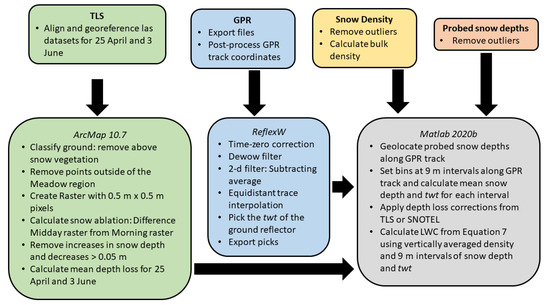
Figure 3.
Schematic diagram of the methods for processing terrestrial laser scanning (TLS), GPR, and field measurements, and calculating LWC.
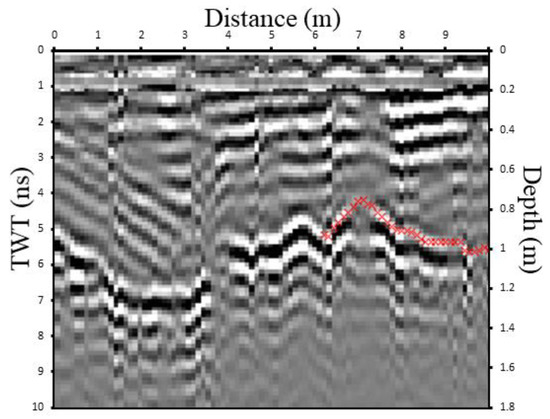
Figure 4.
Processed radargram from the midday North Transect survey on 19 June 2019. The bright white reflector, that varies from 4 to 7 ns depth was identified as the snow–ground interface, as the reflector’s brightness indicates a large shift in permittivity. We picked this continuous reflector, as is noted by the red line. Depth was calculated using a radar velocity of 0.14 m ns−1.
The real component of snow permittivity, as defined by a three-phase mixing formula [65], is defined as:
where is the bulk dry snow density (kg m−3), is the density of ice (kg m−3), LWC is the % volumetric (vol.) liquid water, and , , and are the known relative permittivities of ice, water, and air, respectively. Snow depth, (m), is calculated from and the measured twt as follows:
Here, we assume that snow density and LWC is vertically integrated in the measured twt, and therefore is a function of the bulk snow density and bulk LWC. Finally, SWE (kg m−2) is calculated as:
where is the density of water.
3.5. TLS Processing
We used repeat terrestrial laser scanning (TLS) surveys of the Meadow and South Transects to measure snow ablation that occurred during the 25 April and 3 June survey dates. TLS surveys were acquired using a Riegl VZ-6000 from 10:00 to 11:00 MDT and 14:00 to 15:00 MDT on 25 April and 3 June. We processed the TLS datasets following a methodology similar to Deems et al. [74]; these steps are outlined in Figure 3. Scans were aligned and georeferenced to the NAD 1983 UTM Projected Coordinate System (EPSG:26913) and a surface classification was completed in ArcMap 10.7 to remove above-snow vegetation from the point cloud, using a surface classification algorithm. The remaining points were rasterized at 0.5 m resolution. We then differenced the lidar-derived digital surface models (DSMs) acquired from 10:00 to 11:00 MDT and those from 14:00 to 15:00 MDT to produce distributed fields of snow depth loss/ablation during a single field day. Erroneous depth loss values, identified as increases in snow depth or decreases in snow depth by >0.05 m, were caused by a scanning position that shifted due to an unstable platform, and were filtered from the analysis. We calculated the mean depth loss throughout the scanned area to subtract from probed snow depths acquired during the Morning surveys of the Meadow and South Transects.
3.6. LWC Calculations
3.6.1. Probed Snow Depth Adjustments
We compared GPR-derived snow depths (using a velocity calculated from density observations; Equations (2) and (3)) with spatially coincident probed depths (n = 73) for the 5 April survey to evaluate our permittivity assumptions. This survey consisted of dry snow conditions, as indicated by subzero temperatures measured in the snowpit. We assume the temperatures measured in this snowpit were representative of the three transects at this time. The GPR-derived snow depths were less than the spatially coincident probed depths by an average of 0.14 ± 0.02 m at the 95% confidence interval established using the t-distribution (Figure 5). Possibilities for this observed GPR–probe difference include the spatial footprint over which the two methods measure the base of the snowpack, the potential for overprobing into a thawed ground surface [75], and possible vegetation mats and/or void spaces beneath the snowpack created by various Salix (willow) species that heavily vegetate the area [76]. The latter would likely allow the probe to penetrate through, whereas the GPR would be sensitive to the snow–vegetation interface. In addition, there is also significant variability in published permittivity–density relations (e.g., [77]), such that permittivity can vary by >10% for a given density depending on which equation is used. To account for the observed probe-GPR difference (Figure 5), which we attribute to some combination of the above reasons, we subtracted 0.14 m from each probed snow depth for all surveys. This correction, based on dry snow conditions, is essential to calculate LWC for later surveys, because these surveys rely on the probe-measured snow depths.
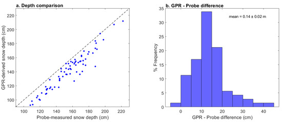
Figure 5.
(a) Probe-measured snow depth compared to GPR-derived snow depths (n = 73). GPR-derived snow depths were calculated using bulk snow density measured in the snowpit and Equation (3). (b) Histogram for the difference between probe-derived snow depths and GPR-derived snow depths. Confidence interval calculated using the t-distribution.
Ablation occurred on 25 April, 3 June, 10 June, and 19 June due to warmer than freezing air temperatures. Because in situ snow depths were acquired during the Morning survey, the snow depths did not accurately reflect the ablating snowpack during the Midday and Evening surveys. Thus, we used two methods to adjust the in situ snow depths to reflect the ablating snowpack. First, we used TLS scans to calculate the mean depth loss (described in Section 3.5) on 25 April (−0.028 m) and 3 June (−0.025 m) in the Meadow and South Transect regions (Figure 6a,b). We applied the mean depth loss uniformly for the Meadow and South Transects. Second, for the 10 June and 19 June surveys, we fit a linear least-squares regression to the Joe Wright SNOTEL hourly snow depths to calculate ablation (Figure 6c,d). The data show scatter, as the accuracy of the SNOTEL sonic depth sensor is ~0.05 m [78], but the 10 June regression has an r2 = 0.4 and a slope estimate = −0.006 m h−1 and the 19 June regression has an r2 = 0.6 and a slope estimate of −0.006 cm h−1. The slopes of these regressions were used to correct the probed depths used for the Midday and Evening surveys. Regressions for other survey dates did not have a strong statistical relation for depth loss, likely due to lower rates of snow depth loss for those dates, and were not used.
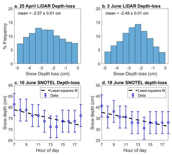
Figure 6.
(a) Snow depth loss histogram for 25 April TLS morning (10:00–11:00 MDT) and midday (14:00–15:00 MDT) surveys. (b) Snow depth loss histogram for 3 June TLS morning and midday surveys. 95% confidence interval calculated using t-distribution. (c) 10 June least-squares regression analysis for snow depth loss plotted with SNOTEL measured depths with 5 cm uncertainty. (d) 19 June least-squares regression analysis for snow depth loss plotted with SNOTEL measured depths with 5 cm uncertainty. Regression performed on hourly Joe Wright SNOTEL station snow depth data between 08:00 and 18:00 MDT.
3.6.2. Constraining Radar Velocity to Calculate LWC
Radar velocity was calculated using coincidently measured snow depths and twt (Equation (4)) and permittivity was calculated from the velocity (Equation (2)). Snowpit-measured density () was unadjusted for LWC and was defined as:
We reformulated Equation (3) with Equation (6) to define LWC as:
This approach is outlined in Figure 3 and is similar to the methodology used by Schmid et al. [54,58] and Webb et al. [57], and assumes the snowpack has spatially varying LWC and snow depth, but is homogeneous with respect to density.
We averaged probed depth measurements and twt over 9 m intervals to minimize the impact of any outlying GPR–probe differences and account for the distinct difference in the spatial footprints of the GPR and probe. In addition, this interval approximates the expected spatial footprint of NISAR. LWC was calculated from transect-specific snowpit density and depth-derived permittivity (Equation (7)). In a few instances, transect-specific snowpits were not available. We thus applied the Meadow Transect density to all transects on 5 April and we averaged the North and South Transect densities for the Meadow Transect on 25 April.
3.7. Synthetic Radar SWE Retrieval Calculations
We first calculated SWE using the adjusted probed snow depths (Section 3.6.1) and snowpit-measured densities (Equation (5)), yielding the best or “true” estimate of SWE, since it accounts for LWC and includes a site-specific estimate of snow density. We generated synthetic SWE retrievals at 9 m intervals from observed twt to investigate the sensitivity of radar SWE retrievals to both LWC and density at the approximated footprint of NISAR, using two methods. Both methods used a velocity based on the assumption that the snow is dry to calculate snow depth from observed twt (Equations (3) and (4)), therefore neglecting the velocity attenuation effect of LWC. The calculated snow depths were then converted to SWE using two different density estimates (Equation (5)): (1) bulk density from snowpit measurements and (2) density calculated from the Joe Wright SNOTEL station. These three methods for calculating SWE highlight the significant impact LWC has on radar velocity, since LWC is not typically measured by automated stations and thus would not be widely available for future spaceborne radar missions.
3.8. Uncertainty in LWC Calculations
Potential measurement errors can arise through snow depth probing, measuring snow density, and picking the ground reflector in radargrams, which affects the uncertainty range for LWC calculations. In depth probing, depths can either be under-probed due to the presence of ice lenses, or over-probed due to a thawed and potentially saturated wet ground surface [75]. Snow density can be under-sampled where ice lenses are present or oversampled in less cohesive intervals [79]. For the GPR, twt errors arise when picking a reflector that is not the ground reflector, or picking the ground reflector when there is a void space between the snowpack and the ground reflector. We estimated uncertainty in LWC calculations through a Monte Carlo analysis. For this calculation, we used the mean values across all survey dates for snow depth (0.82 m), density (439 kg m−3), and twt (9.13 ns). We assume errors are normally distributed and have a standard deviation equal to ±0.05 m for probed snow depths [75], ±5% for bulk density [79], and four samples for twt (0.4 ns). The three variables are sampled 100,000 times assuming a random normal distribution. The standard deviation of LWC for this Monte Carlo analysis is ~2.4 vol. %, which we use as the uncertainty range for our calculations. Negative LWC values were calculated for ~1% of the dataset. These values were within the uncertainty range and were corrected to 0 vol. % since negative LWC is not physically realistic.
4. Results
4.1. Overview of the Study Period
On the 5 April survey, snow temperatures in the snowpit ranged from 0 °C near the ground to –3.1 °C at the surface. The mean snow temperature was −0.9 °C, and the upper 0.8 m of the snowpack had a temperature <–1.0 °C. Ice lenses were absent, but a ~0.03 m melt-freeze crust was present at the surface. These observations indicate that LWC was negligible. By 25 April, observed snowpits were isothermal at 0 °C and we noted multiple ice lenses, indicating that significant melt had occurred in the prior 20 days. However, between this date and 6 June, a series of late-season storms impacted the study site, each adding SWE that partially offset prior melt and caused SWE at the Joe Wright SNOTEL station to remain within 20% of peak SWE, which occurred previously on 18 April. During this interval, the mean basin-wide melt rate calculated from the Joe Wright Stream gauge was 1.3 mm water equivalent (WE) day−1. From 7 June to 30 June, the end of the melt season, melt occurred more rapidly at a mean rate of 14.9 mm WE day−1 (Figure 7). The 2019 melt season lasted 73 days, which is 27 days longer than the 1978–2018 average. This longer than normal melt season is attributed to two factors: (1) temperatures in May and June were cooler than the 1978–2018 average temperatures by about 1.4 °C and (2) there were six late-season storm events that each added >10 mm of SWE (Table 2), each causing an inferred increase in albedo. Collectively, these factors delayed SWE loss and the corresponding increase in stream discharge until after 1 June. Light rainfall was observed on the afternoons of 4 June and 10 June, but was not recorded by the SNOTEL station.
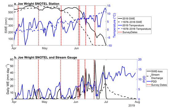
Figure 7.
(a) Joe Wright SNOTEL station 2019 daily observations of SWE and average air temperature, compared with 1978–2018 daily averages. (b) Joe Wright SNOTEL station 2019 hourly air temperatures, converted to PDD, compared with SWE loss from Joe Wright SNOTEL station and stream discharge from Joe Wright Creek stream gauge, converted to water equivalent (WE). Michigan Ditch stream gauge data was subtracted from Joe Wright Stream gauge to remove regulated inflow.
Table 2.
Late-season storm events recorded at the Joe Wright SNOTEL Station for the 2019 season.
4.2. In Situ Observations
Snow depth values, within published accuracies (±0.05 m; [75]), decreased throughout the spring (Figure 8). The highest median snow depths were observed on the North Transect (Figure 9a), while the Meadow (Figure 9b) and South (Figure 9c) Transects displayed similar snow depth ranges and medians. Higher snow depths were observed over the first 25 m of the north ends of the Meadow and South Transects, likely due to additional deposition by snowplow operations along the road.
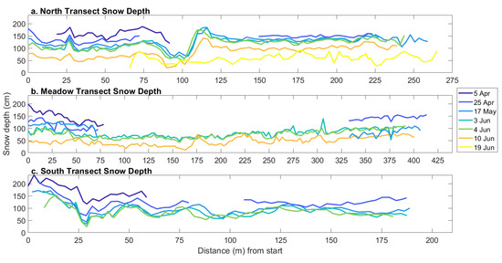
Figure 8.
Probed snow depth measurements on the (a) North, (b) Meadow, and (c) South Transects. Snow depths on 5 April (a–c), 25 April (a–c), and 17 May (b) surveys were acquired on a subset of the transect. Transect terminus varied by up to 5 m in length throughout the survey period.
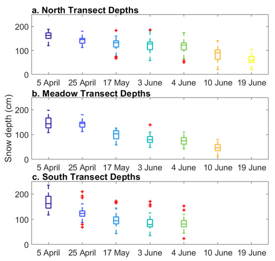
Figure 9.
Boxplots displaying probed snow depth variability for the (a) North, (b) Meadow, and (c) South Transects. The boxes extend to the upper and lower quartiles, while the whiskers extend to extreme values not considered outliers. Red crosses denote outliers.
Temporal changes in snow density differed for each transect (Figure 10). Snow density on the North Transect generally increased throughout the season and closely resembled the Joe Wright SNOTEL density (mean absolute difference = 6%), with two of the initial surveys yielding higher densities than the SNOTEL station and the final four surveys yielding lower densities. For the Meadow Transect, density increased from 5 April to 3 June and then decreased for each subsequent survey date. Meadow Transect densities also followed Joe Wright SNOTEL densities closely (mean absolute difference = 6%), with three surveys yielding greater densities than the SNOTEL station and two surveys yielding lower densities. The largest difference occurred late in the melt season (10 June difference = 11%). South Transect densities decreased from 25 April to 3 June, showing an opposite trend than the other transects and Joe Wright SNOTEL densities (mean difference = 9%).
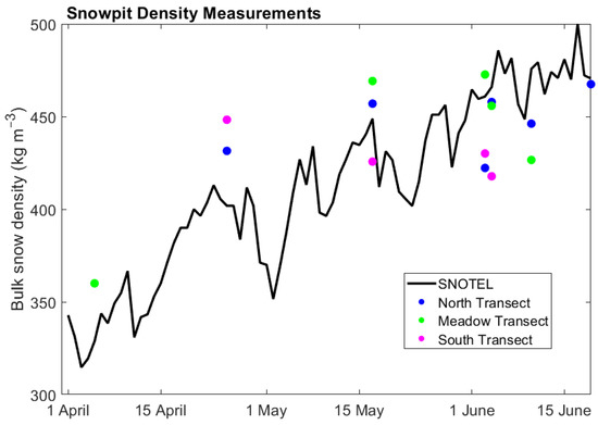
Figure 10.
Snowpit density measurements compared with Joe Wright SNOTEL station density observations. The Meadow Transect snowpit was the only snowpit dug for 5 April.
4.3. GPR-Derived LWC
LWC calculated along the North Transect (Figure 11a) was 0 vol. % on 5 April. Median values for morning surveys (Table 3) increased by survey date from 0 vol. % on 5 April to 3.2 vol. % on 3 June, decreased to 2.4 vol. % on 10 June, and increased to 5.4 vol. % on 19 June. The median ΔLWC (Figure 11b) from morning to midday was positive on 25 April (+0.2 vol. %) and 10 June (+1.1 vol. %), negative on 4 June (−0.7 vol. %), and 19 June (−0.2 vol. %), and negligible on 3 June (0 vol. %). The median ΔLWC from midday to evening was negative for 25 April (−0.2 vol. %), 4 June (−0.1 vol. %), 10 June (−0.5 vol. %), and 19 June (−0.2 vol. %). The interquartile range for ΔLWC was smallest for morning to midday on 25 April (0.4 vol. %) and largest for midday to evening on 10 June (2.1 vol. %). For every morning survey, observed LWC at the southern end (0−50 m), where the transect crosses an open meadow, was consistently higher than the survey’s median LWC value. The highest LWC values were observed on 19 June (11.5 vol. %).
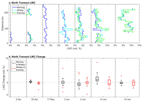
Figure 11.
(a) North Transect LWC averaged along 9 m intervals for morning, midday, and evening surveys, plotted with distance along transect. Explainable outliers were removed and are represented as breaks in the line. (b) Boxplots of ΔLWC along the North Transect from morning to midday and from midday to evening. Positive values represent an increase in LWC, and negative values represent a decrease in LWC. The 3 June evening survey GPR track exhibited poor GPS quality and was not included in the analysis.
Table 3.
Morning survey median vol. % LWC by transect.
LWC calculated along the Meadow Transect (Figure 12a) was 0 vol. % on 5 April and generally increased throughout the observation period. Median values for morning surveys (Table 3) increased from 5 April to 17 May, decreased from 17 May to 3 June, and increased from 3 June to 10 June. The median ΔLWC (Figure 12b) from morning to midday was positive on 25 April (+0.8 vol. %), 3 June (+1.6 vol. %), and 10 June (+1.2 vol. %), and negligible on 4 June (~0 vol. %). The median ΔLWC from midday to evening was negative on 25 April (−0.3 vol. %), 3 June (−1.1 vol. %), 4 June (−0.5 vol. %), and 10 June (−0.3 vol. %). The ΔLWC interquartile range increased significantly on the 10 June surveys to 3.3 vol. % for morning to midday and 1.9 vol. % for midday to evening. Observed LWC at the northern (Figure 12a, 0−50 m) and southern (Figure 12a, 350−400 m) ends of the transect were consistently greater than the survey’s median for every date, except 10 June, when LWC values at the southern end were less than the survey’s median. In the middle region, where the transect crosses the stream twice, we observed lower LWC values at the start of the season, but this region’s LWC progressively developed such that it contained the highest LWC values across all transects. The highest LWC values were observed on 10 June (maximum = 19.5 vol. %) at a location close to the stream and at a time when the near-surface soil was saturated such that 0.05 m of standing water was observed in the snowpit.
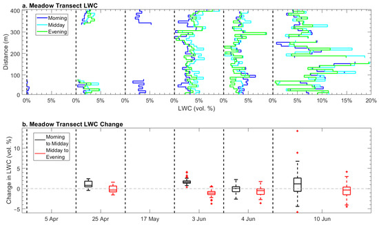
Figure 12.
(a) Meadow Transect LWC averaged along 9 m intervals for morning, midday, and evening surveys, plotted with distance along transect. Explainable outliers were removed and are represented as breaks in the line. (b) Box plots of ΔLWC along the Meadow Transect from morning to midday and from midday to evening. Positive values represent an increase in LWC, and negative values represent a decrease in LWC.
Median LWC calculated along the South Transect (Figure 13a) was <1 vol. % on 5 April and progressively increased during the observation period (Table 3). The median ΔLWC (Figure 13b) from morning to midday was positive on 25 April (+0.4 vol. %) and negative on 3 June (−0.1 vol. %) and 4 June (−1.7 vol. %). The median ΔLWC from midday to evening was negative on 25 April (−0.3 vol. %), 3 June (−0.2 vol. %), and negligible on 4 June (~0 vol. %). The highest LWC values were observed on 3 June (maximum = 11 vol. %), on a forested, south-facing slope at ~60 m distance from the western terminus of the transect (a. on Figure 2), where surface slopes are lower and the transect moves out of canopy cover and crosses into an open meadow. Here, we observed LWC values that exceeded the morning survey’s median LWC value for every survey date except 5 April, when LWC in this region was observed at 0 vol. %.
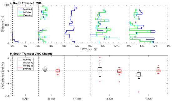
Figure 13.
(a) South Transect LWC averaged along 9 m intervals for morning, midday, and evening surveys, plotted with distance along transect. Explainable outliers were removed and are represented as breaks in the line. (b) Box plots of ΔLWC along the South Transect from morning to midday and from midday to evening, where positive values represent an increase in LWC, and negative values represent a decrease in LWC.
4.4. Sensitivity of Synthetic Radar SWE Retrievals to LWC
We explored the sensitivity of synthetic SWE retrievals to LWC based on the snowpit densities and the Joe Wright SNOTEL station density, neglecting the velocity attenuation effects of LWC (Figure 14). In the dry snow conditions of 5 April, the synthetic SWE retrievals using snowpit-measured density underestimate SWE by a mean of 1%, while synthetic SWE retrievals that use the SNOTEL density overestimate SWE by a mean of 6%. In all surveys after 5 April (i.e., when LWC was present in the snowpack), the use of the dry snow density model for permittivity overestimated SWE by a mean of 16 and 18% for the snowpit and SNOTEL densities, respectively. The disagreement increased throughout the season, reflecting the increase in LWC, and at its maximum, resulted in a 40% overestimation of SWE. In a few cases, synthetic SWE retrievals using SNOTEL densities are closer to the true SWE, resulting from SNOTEL densities that were higher than snowpit densities, causing higher permittivity values/lower velocities. Snow pillows have an impermeable surface that could result in ponding water at the base of the snowpack during the melt season, thereby yielding increased density measurements.
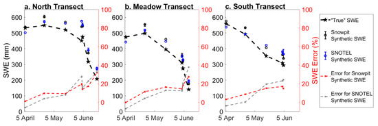
Figure 14.
SWE calculations from probe and snowpit datasets (“True” SWE) compared to synthetic SWE retrievals based on a 0 vol. % LWC assumption for snowpit densities and SNOTEL densities. Percent error shown in red represents the synthetic SWE retrievals using the local snowpit density. Percent error shown in gray represents the synthetic SWE retrievals using the Joe Wright SNOTEL station density. Percent error given as the mean percent error from the transect.
5. Discussion
5.1. Variability in GPR and In Situ Observations
5.1.1. Temporal Variability
Snowpit-measured bulk density showed opposing seasonal patterns between the three transects, with the peak observed density occurring first on the South Transect (25 April), then on the Meadow Transect (3 June), and last on the North Transect (19 June). The South Transect snowpit densities declined throughout our field surveys. The highest SWE observed (Figure 14) on the South Transect was observed on 5 April, which contrasts with the North and Meadow Transects, where we recorded our highest SWE observations on 25 April. This indicates that the snowpack in this area likely ripened earlier than other transects due to a more positive net energy balance related to its slope and aspect, and likely developed preferential flowpaths [80], which drained meltwater through the snowpack and lowered the density [53]. The North Transect density was lower than the South Transect density on 25 April and the Meadow Transect density on 17 May. This agrees with Rasmus [81], who found that snowpack density is lower in forested plots than in open plots. In contrast to this initial relation, we found that the snowpits on the Meadow and South Transects, which were in the open, had lower densities than the North Transect snowpits after significant SWE losses in the open. We infer that more efficient flowpaths developed in the open areas, due to higher exposure to shortwave radiation causing increased melt rates.
The Meadow and South Transects exhibited consistent diurnal LWC variability, such that ~60% (7 of 12) of morning to midday intervals (Figure 12, Figure 13 and Figure 14) exhibited positive median ΔLWC and 100% of midday to evening intervals exhibited negative median ΔLWC. This result is expected, as incoming shortwave radiation, a primary driver of LWC development, increases from morning to midday and decreases from midday to evening [82]. Similar increases in plot-scale LWC from 12:40 to 15:00 MDT were observed by Webb et al. [56] at an alpine site in central Colorado, with a subsequent overnight decline in LWC effectively resetting its distribution. Limited diurnal variability during the early part of the melt season was observed at Davos, Switzerland [54] and in Boise, Idaho, USA [43] when air temperatures were ~0 °C. Later in the season, both studies observed diurnal fluctuations that were typified by an LWC increase in 1−2 vol. % when daytime air temperatures were 5−12 °C, and a decrease of 1−2 vol. % overnight when air temperatures dropped, but rarely to 0 °C. At our site, the median diurnal variability from 25 April to 4 June and on 19 June was limited in magnitude. This is likely explained by the lower air temperatures observed at our site and the presence of canopy on two of our transects, which would attenuate shortwave radiation and strongly influence the snowpack energy balance [83,84].
5.1.2. Spatial Variability
In this study, we considered only the lateral spatial variability of LWC, since the measured twt integrates the vertical variability of LWC. Median LWC values did not exceed 7 vol. % on any of the field surveys. This is comparable to the findings of Webb et al. [57], who presented spatially variable LWC values for two survey dates in May 2017 that did not exceed 10 vol. % and had means of ~4 vol. %. In our study, LWC standard deviation exceeded 2.0 vol. % on three morning surveys: 4 June South Transect (standard deviation = 3.0 vol. %), 10 June Meadow Transect (standard deviation = 5.8 vol. %), and 19 June North Transect (standard deviation = 2.7 vol. %). Notably, these were the last dates that surveys were performed on the transects, as melt-out occurred prior to the next survey. This suggests that LWC variability may be fairly limited during longer-than-average melt seasons at sites similar to our field site. Contrary to our expectations, we found comparable LWC between our South and Meadow Transects. The median South Transect LWC values were within 0.4 vol. % of the median Meadow Transect LWC values until 3 June. On 4 June, the South Transect median LWC was 2.9 vol. % less than the Meadow Transect median. The South Transect had higher maximum LWC values for only three of its five survey dates (5 April, 3 June, and 4 June), even though the snow depth declined more rapidly on the South Transect during the study interval, which suggests a higher rate of ablation along this transect. We propose that the lack of aspect-related LWC differences between these transects can be attributed to two primary factors: (1) differences in surface slope and (2) the proximity of the stream to the Meadow Transect. The Meadow Transect has a ~0° slope and parallels and crosses the stream, where ground saturation and streamflow likely saturated the base of the snowpack and inhibited water drainage to the snow–ground interface, whereas the steeper slopes of the South Transect likely aided in drainage development at the base of the snowpack and along dipping snow stratigraphic layers [50,85]. Thus, any aspect related differences in meltwater production were compensated for by differences in meltwater drainage.
Snow depths declined more slowly on the North Transect than the other transects and LWC values were consistently lower along the 150 m section, which follows a narrow alley where canopy cover is 50–70%, than the 75 m section which is in open canopy. This variability was likely caused by the modulation of incoming shortwave radiation by canopy cover (e.g., [56,83]). The highest LWC values for the North Transect were observed on 19 June, the day prior to the highest 24-h SWE-loss recorded at the Joe Wright SNOTEL station during the 2019 season (Figure 8b). In this case, the near-surface soil was saturated and standing water was observed at 0.05 m height in the snowpit, suggesting that the base of the snowpack was saturated and likely prevented output of meltwater. This was also reflected by the stream gauge, which recorded higher discharge than the SNOTEL reported SWE-loss for two days prior to 19 June. The highest LWC values for the Meadow Transect were observed in the middle portion, where it crosses the stream channel. Here, early-season streamflow, likely starting on 16 May when the stream gauge recorded WE-loss that exceeded base flow, saturated the base of the snowpack. Less than 4% of our observations of LWC were greater than 10 vol. % during the 2019 season. These instances include observations near the melt out date, near a stream, or where topographic lows and saturated ground prevent meltwater drainage from the snowpack [56]. However, LWC development exhibits year-to-year variability and is influenced by temperature trends and late-season storms [43], and since the 2019 melt season at Cameron Pass was >50% longer than average and characterized by less-than-average air temperatures, meltwater production/output was likely lower than during years characterized by a shorter duration and more intense melt season. Thus, the isolated instances of ground saturation leading to elevated LWC values at the base of the snowpack would perhaps be more expansive during other years.
5.2. Implications for Radar Remote Sensing
Spatiotemporal variability in density is a significant source of uncertainty in depth-based SWE retrievals [86], but less so for radar-based methods, as radar velocity is less sensitive to density variations (e.g., [29,87]). Our density measurements showed good agreement (mean difference = 6%; Figure 10) with the Joe Wright SNOTEL station, which supports the use of SNOTEL station density observations for estimating radar velocity in small basins [88,89], although there may be larger variations on slopes due to more complex terrain, as two of the three snowpits and the SNOTEL station are located in flat terrain. Furthermore, in cases where the SNOTEL density varied more considerably from the snowpit density (e.g., the 9% mean difference observed across all survey dates on the South Transect), the impact that density has on SWE retrievals is less than the impact of LWC.
If LWC is present in the snowpack but not explicitly accounted for in the SWE retrievals, the actual SWE on the ground will be overestimated (Figure 14). As the melt-season progressed, greater LWC values produced larger errors in the synthetic SWE retrievals, demonstrating that, in wet snow, the use of a velocity based solely on dry snow density would add significant uncertainty to the identification of the peak SWE date, the progression of the melt season, and the monitoring of remaining SWE for water resources. In this analysis, the highest observed SWE on the South Transect occurred on 5 April and for the North and Meadow Transects on 25 April (Joe Wright SNOTEL station peak SWE was observed on 18 April). The synthetic SWE retrievals, which do not account for the presence of LWC, observe negligible SWE change between 25 April and 3 June on the North Transect, whereas “true” SWE, informed by LWC calculations, decreased by 18%. The highest mean percent error is 38%, observed on the Meadow Transect on 10 June (using SNOTEL density). These results indicate that radar SWE retrievals, in the absence of supporting observations, are most suitable to dry snow conditions and that significant caution is required when interpreting retrievals during the melt-season even when coherence is maintained.
Typically, LWC was lowest during the morning surveys, peaked during midday surveys, and dropped during evening surveys. Lower LWC during morning surveys resulted from below-freezing overnight temperatures and lower amounts of shortwave radiation at this time of day. Lower LWC during evening surveys resulted from declining air temperatures and a reduction in incoming shortwave radiation. Collectively, these observations indicate that the diurnal variability of LWC is an important factor to consider when trying to minimize the uncertainty of radar SWE retrievals [87]. NISAR, with its planned dawn-dusk overpasses, is aligned optimally with when snowpack LWC is at a minimum. However, as we have shown, low LWC values can still introduce error into radar SWE retrievals. Therefore, as methods for using InSAR to measure SWE continue to develop, previously established methods for identifying wet snow from SAR imagery (e.g., [33]) may be useful for establishing regions of higher SWE uncertainty.
6. Conclusions
In our study, we examined the diurnal and seasonal variability of bulk LWC using GPR, snow depths, and bulk snow density acquired along three transects with varying aspect, slope, and canopy cover in a continental snow climate. During this cooler than average melt season, median LWC remained below 7 vol. % on all transects from 5 April to 19 June. Less than 4% of the calculated LWC values exceeded 10 vol. % and were observed on and after 4 June, and usually in areas where a saturated ground limited further meltwater output. LWC varied from morning to midday by 0.5–1.5 vol. % and from midday to evening by –1.0–0.0 vol. %. The open meadows on the Meadow and South Transects exhibited identical LWC values despite different ablation rates. We suggest the similarity for LWC values is likely caused by differences in drainage efficiency. On the North Transect, which is forested, LWC values were lower than open areas, highlighting the important role of canopy cover for modulating shortwave radiation. The presence of LWC can result in upwards of a ~40% overestimation of SWE using phase-based radar techniques late in the season, but even moderate LWC (e.g., 5–7 vol. %) values can cause significant uncertainty in radar SWE retrievals. Continued research on the spatiotemporal patterns of LWC development is essential in order to fully realize the potential of spaceborne radar based SWE retrievals.
Author Contributions
Conceptualization, R.B., D.M., R.W. and H.-P.M.; Methodology, R.B., D.M., R.W., S.R.F., K.W. and H.-P.M.; Software, R.B. and D.M.; Validation, R.B. and D.M.; Formal Analysis, R.B., D.M., K.W. and S.R.F.; Investigation, R.B. and D.M.; Resources, D.M.; Data Curation, R.B., D.M., and K.W.; Writing—Original Draft Preparation, R.B.; Writing—Review and Editing, R.B., D.M., S.R.F., R.W., H.-P.M. and K.W.; Visualization, R.B., D.M. and S.R.F.; Supervision, D.M.; Project Administration, D.M.; Funding Acquisition, D.M., H.-P.M. and R.W. All authors have read and agreed to the published version of the manuscript.
Funding
R.B., D.M., R.W. and H.-P.M. acknowledge NASA THP award 80NSSC18K0877. R.B acknowledges NASA FINESST award 80NSSC20K1624 for support.
Institutional Review Board Statement
Not Applicable.
Informed Consent Statement
Not Applicable.
Data Availability Statement
Lidar data are available through UNAVCO at https://doi.org/10.7283/048n-jw94 for 25 April 2019 and https://doi.org/10.7283/j4rf-2924 for 3 June 2019. Last accessed 29 April 2020. Raw GPR data, in situ observations, and calculated liquid water content values are available through Mountain Scholar at https://hdl.handle.net/10217/233636. Last accessed 1 September 2021.
Acknowledgments
We thank Caroline Duncan, Will Gnesda, Tyler Miller, Alex Olsen-Mikitowicz, and Brianna Rick for their fieldwork contributions. We acknowledge the services provided by the GAGE Facility, operated by UNAVCO, Inc., with support from the National Science Foundation and the National Aeronautics and Space Administration under NSF Cooperative Agreement EAR-1724794. Additionally, we would like to thank three anonymous reviewers and the Editor, Ana Barros, for providing valuable suggestions which helped improve the clarity of this work.
Conflicts of Interest
The authors declare no conflict of interest.
References
- Hammond, J.C.; Saavedra, F.A.; Kampf, S.K. Global snow zone maps and trends in snow persistence 2001–2016. Int. J. Clim. 2018, 38, 4369–4383. [Google Scholar] [CrossRef]
- Kim, E. How Can We Find Out How Much Snow Is in the World? Eos 2018, 99. [Google Scholar] [CrossRef]
- Warren, S.G. Optical properties of snow. Rev. Geophys. 1982, 20, 67–89. [Google Scholar] [CrossRef]
- Doesken, N.; Judson, A. The Snow Booklet: A Guide to the Science, Climatology, and Measurement of Snow in the United States; Colorado State University: Fort Collins, CO, USA, 1996; p. 86. [Google Scholar]
- Barnett, T.P.; Adam, J.C.; Lettenmaier, D.P. Potential impacts of a warming climate on water availability in snow-dominated regions. Nature 2005, 438, 303–309. [Google Scholar] [CrossRef]
- Keller, F.; Goyette, S.; Beniston, M. Sensitivity Analysis of Snow Cover to Climate Change Scenarios and Their Impact on Plant Habitats in Alpine Terrain. Clim. Chang. 2005, 72, 299–319. [Google Scholar] [CrossRef]
- Niittynen, P.; Heikkinen, R.K.; Luoto, M. Snow cover is a neglected driver of Arctic biodiversity loss. Nat. Clim. Chang. 2018, 8, 997–1001. [Google Scholar] [CrossRef]
- Pepin, N.; Bradley, R.S.; Diaz, H.F.; Baraer, M.; Caceres, E.B.; Forsythe, N.; Fowler, H.; Greenwood, G.; Hashmi, M.Z.; Liu, X.D.; et al. Elevation-dependent warming in mountain regions of the world. Nat. Clim. Chang. 2015, 5, 424–430. [Google Scholar] [CrossRef]
- Huang, J.; Zhang, X.; Zhang, Q.; Lin, Y.; Hao, M.; Luo, Y.; Zhao, Z.; Yao, Y.; Chen, X.; Wang, L.; et al. Recently amplified arctic warming has contributed to a continual global warming trend. Nat. Clim. Chang. 2017, 7, 875–879. [Google Scholar] [CrossRef]
- Dettinger, M.D.; Cayan, D.R.; Meyer, M.K.; Jeton, A.E. Simulated Hydrologic Responses to Climate Variations and Change in the Merced, Carson, and American River Basins, Sierra Nevada, California, 1900–2099. Clim. Chang. 2004, 62, 283–317. [Google Scholar] [CrossRef]
- Stewart, I.T.; Cayan, D.R.; Dettinger, M.D. Changes toward Earlier Streamflow Timing across Western North America. J. Clim. 2005, 18, 1136–1155. [Google Scholar] [CrossRef]
- Clow, D. Changes in the Timing of Snowmelt and Streamflow in Colorado: A Response to Recent Warming. J. Clim. 2010, 23, 2293–2306. [Google Scholar] [CrossRef]
- Hall, D.K.; Crawford, C.J.; DiGirolamo, N.E.; Riggs, G.A.; Foster, J.L. Detection of earlier snowmelt in the Wind River Range, Wyoming, using Landsat imagery, 1972–2013. Remote Sens. Environ. 2015, 162, 45–54. [Google Scholar] [CrossRef]
- Mote, P.W.; Li, S.; Lettenmaier, D.P.; Xiao, M.; Engel, R. Dramatic declines in snowpack in the western US. Npj Clim. Atmos. Sci. 2018, 1. [Google Scholar] [CrossRef]
- Estilow, T.W.; Young, A.H.; Robinson, D.A. A long-term Northern Hemisphere snow cover extent data record for climate studies and monitoring. Earth Syst. Sci. Data 2015, 7, 137–142. [Google Scholar] [CrossRef]
- Klos, P.Z.; Link, T.E.; Abatzoglou, J.T. Extent of the rain-snow transition zone in the western U.S. under historic and projected climate. Geophys. Res. Lett. 2014, 41, 4560–4568. [Google Scholar] [CrossRef]
- Kirkham, J.D.; Koch, I.; Saloranta, T.M.; Litt, M.; Stigter, E.E.; Møen, K.; Thapa, A.; Melvold, K.; Immerzeel, W.W. Near Real-Time Measurement of Snow Water Equivalent in the Nepal Himalayas. Front. Earth Sci. 2019, 7. [Google Scholar] [CrossRef]
- Livneh, B.; Badger, A.M. Drought less predictable under declining future snowpack. Nat. Clim. Chang. 2020, 10, 452–458. [Google Scholar] [CrossRef]
- Dozier, J.; Bair, E.H.; Davis, R.E. Estimating the spatial distribution of snow water equivalent in the world’s mountains. Wiley Interdiscip. Rev. Water 2016, 3, 461–474. [Google Scholar] [CrossRef]
- Takala, M.; Luojus, K.; Pulliainen, J.; Derksen, C.; Lemmetyinen, J.; Kärnä, J.-P.; Koskinen, J.; Bojkov, B. Estimating northern hemisphere snow water equivalent for climate research through assimilation of space-borne radiometer data and ground-based measurements. Remote Sens. Environ. 2011, 115, 3517–3529. [Google Scholar] [CrossRef]
- Mote, T.L.; Grundstein, A.J.; Leathers, D.J.; Robinson, D.A. A comparison of modeled, remotely sensed, and measured snow water equivalent in the northern Great Plains. Water Resour. Res. 2003, 39. [Google Scholar] [CrossRef]
- Shi, J.; Xiong, C.; Jiang, L. Review of snow water equivalent microwave remote sensing. Sci. China Earth Sci. 2016, 59, 731–745. [Google Scholar] [CrossRef]
- Pulliainen, J.; Luojus, K.; Derksen, C.; Mudryk, L.; Lemmetyinen, J.; Salminen, M.; Ikonen, J.; Takala, M.; Cohen, J.; Smolander, T.; et al. Patterns and trends of Northern Hemisphere snow mass from 1980 to 2018. Nat. Cell Biol. 2020, 581, 294–298. [Google Scholar] [CrossRef]
- Painter, T.H.; Berisford, D.F.; Boardman, J.W.; Bormann, K.J.; Deems, J.; Gehrke, F.; Hedrick, A.; Joyce, M.; Laidlaw, R.; Marks, D.; et al. The Airborne Snow Observatory: Fusion of scanning lidar, imaging spectrometer, and physically-based modeling for mapping snow water equivalent and snow albedo. Remote Sens. Environ. 2016, 184, 139–152. [Google Scholar] [CrossRef]
- Currier, W.R.; Pflug, J.; Mazzotti, G.; Jonas, T.; Deems, J.S.; Bormann, K.J.; Painter, T.H.; Hiemstra, C.A.; Gelvin, A.; Uhlmann, Z.; et al. Comparing Aerial Lidar Observations with Terrestrial Lidar and Snow-Probe Transects from NASA’s 2017 SnowEx Campaign. Water Resour. Res. 2019, 55, 6285–6294. [Google Scholar] [CrossRef]
- Shean, D.; Alexandrov, O.; Moratto, Z.M.; Smith, B.E.; Joughin, I.; Porter, C.; Morin, P. An automated, open-source pipeline for mass production of digital elevation models (DEMs) from very-high-resolution commercial stereo satellite imagery. ISPRS J. Photogramm. Remote Sens. 2016, 116, 101–117. [Google Scholar] [CrossRef]
- Shaw, T.; Gascoin, S.; Mendoza, P.A.; Pellicciotti, F.; McPhee, J. Snow Depth Patterns in a High Mountain Andean Catchment from Satellite Optical Tristereoscopic Remote Sensing. Water Resour. Res. 2020, 56. [Google Scholar] [CrossRef]
- Eberhard, L.A.; Sirguey, P.; Miller, A.; Marty, M.; Schindler, K.; Stoffel, A.; Bühler, Y. Intercomparison of photogrammetric platforms for spatially continuous snow depth mapping. Cryosphere 2021, 15, 69–94. [Google Scholar] [CrossRef]
- McGrath, D.; Webb, R.; Shean, D.; Bonnell, R.; Marshall, H.; Painter, T.H.; Molotch, N.P.; Elder, K.; Hiemstra, C.; Brucker, L. Spatially Extensive Ground-Penetrating Radar Snow Depth Observations During NASA’s 2017 SnowEx Campaign: Comparison with In Situ, Airborne, and Satellite Observations. Water Resour. Res. 2019, 55, 10026–10036. [Google Scholar] [CrossRef]
- Harder, P.; Pomeroy, J.W.; Helgason, W.D. Improving sub-canopy snow depth mapping with unmanned aerial vehicles: Lidar versus structure-from-motion techniques. Cryosphere 2020, 14, 1919–1935. [Google Scholar] [CrossRef]
- Deeb, E.J.; Forster, R.R.; Kane, D.L. Monitoring snowpack evolution using interferometric synthetic aperture radar on the North Slope of Alaska, USA. Int. J. Remote Sens. 2011, 32, 3985–4003. [Google Scholar] [CrossRef]
- Marshall, H.P.; Deeb, E.; Forster, R.; Vuyovich, C.; Elder, K.; Hiemstra, C.; Lund, J. L-band InSAR depth retrieval during the NASA SnowEx 2020 campaign: Grand Mesa, Colorado. In Proceedings of the IEEE International Geoscience and Remote Sensing Symposium, Brussels, Belgium, 11–16 July 2021; pp. 625–627. [Google Scholar] [CrossRef]
- Lund, J.; Forster, R.R.; Rupper, S.B.; Deeb, E.J.; Marshall, H.P.; Hashmi, M.Z.; Burgess, E. Mapping Snowmelt Progression in the Upper Indus Basin with Synthetic Aperture Radar. Front. Earth Sci. 2020, 7. [Google Scholar] [CrossRef]
- Huning, L.S.; AghaKouchak, A. Approaching 80 years of snow water equivalent information by merging different data streams. Sci. Data 2020, 7, 333. [Google Scholar] [CrossRef]
- Koch, F.; Prasch, M.; Schmid, L.; Schweizer, J.; Mauser, W. Measuring Snow Liquid Water Content with Low-Cost GPS Receivers. Sensors 2014, 14, 20975–20999. [Google Scholar] [CrossRef]
- Dozier, J.; Shi, J. Estimation of snow water equivalence using SIR-C/X-SAR. I. Inferring snow density and subsurface properties. IEEE Trans. Geosci. Remote Sens. 2000, 38, 2465–2474. [Google Scholar] [CrossRef]
- Moller, D.; Andreadis, K.M.; Bormann, K.J.; Hensley, S.; Painter, T.H. Mapping Snow Depth from Ka-Band Inter-ferometry: Proof of Concept and Comparison with Scanning Lidar Retrievals. IEEE Geosci. Remote Sens. Lett. 2017, 14, 886–890. [Google Scholar] [CrossRef]
- Tsai, Y.-L.S.; Dietz, A.; Oppelt, N.; Kuenzer, C. Remote Sensing of Snow Cover Using Spaceborne SAR: A Review. Remote Sens. 2019, 11, 1456. [Google Scholar] [CrossRef]
- Lievens, H.; Demuzere, M.; Marshall, H.-P.; Reichle, R.H.; Brucker, L.; Brangers, I.; De Rosnay, P.; Dumont, M.; Girotto, M.; Immerzeel, W.W.; et al. Snow depth variability in the Northern Hemisphere mountains observed from space. Nat. Commun. 2019, 10, 4629. [Google Scholar] [CrossRef] [PubMed]
- Marshall, H.P.; Vuyovich, C.; Hiemstra, C.; Brucker, L.; Elder, K.; Deems, J.; Newlin, J. NASA SnowEx 2020 Experiment Plan (Science Plan). 2019. Available online: https://snow.nasa.gov/campaigns/snowex/experimental-plan-2021 (accessed on 23 June 2020).
- Manickam, S.; Barros, A. Parsing Synthetic Aperture Radar Measurements of Snow in Complex Terrain: Scaling Behaviour and Sensitivity to Snow Wetness and Landcover. Remote Sens. 2020, 12, 483. [Google Scholar] [CrossRef]
- Lundberg, A.; Richardson-Näslund, C.; Andersson, C. Snow density variations: Consequences for ground-penetrating radar. Hydrol. Process. 2005, 20, 1483–1495. [Google Scholar] [CrossRef]
- Heilig, A.; Mitterer, C.; Schmid, L.; Wever, N.; Schweizer, J.; Marshall, H.; Eisen, O. Seasonal and diurnal cycles of liquid water in snow—Measurements and modeling. J. Geophys. Res. Earth Surf. 2015, 120, 2139–2154. [Google Scholar] [CrossRef]
- Koh, G.; Yankielun, N.E.; Baptista, A.I. Snow Cover Characterization Using Multiband Fmcw Radars. Hydrol. Process. 1996, 10, 1609–1617. [Google Scholar] [CrossRef]
- Marshall, H.-P.; Koh, G. FMCW radars for snow research. Cold Reg. Sci. Technol. 2008, 52, 118–131. [Google Scholar] [CrossRef]
- Guneriussen, T.; Hogda, K.; Johnsen, H.; Lauknes, I. InSAR for estimation of changes in snow water equivalent of dry snow. IEEE Trans. Geosci. Remote Sens. 2001, 39, 2101–2108. [Google Scholar] [CrossRef]
- Cline, D.W. Snow surface energy exchanges and snowmelt at a continental, midlatitude Alpine site. Water Resour. Res. 1997, 33, 689–701. [Google Scholar] [CrossRef]
- McCabe, G.J.; Clark, M.P.; Hay, L.E. Rain-on-Snow Events in the Western United States. Bull. Am. Meteorol. Soc. 2007, 88, 319–328. [Google Scholar] [CrossRef]
- Jennings, K.S.; Kittel, T.G.F.; Molotch, N.P. Observations and simulations of the seasonal evolution of snowpack cold content and its relation to snowmelt and the snowpack energy budget. Cryosphere 2018, 12, 1595–1614. [Google Scholar] [CrossRef]
- Eiriksson, D.; Whitson, M.; Luce, C.H.; Marshall, H.P.; Bradford, J.; Benner, S.G.; Black, T.; Hetrick, H.; McNamara, J.P. An evaluation of the hydrologic relevance of lateral flow in snow at hillslope and catchment scales. Hydrol. Process. 2013, 27, 640–654. [Google Scholar] [CrossRef]
- Webb, R.W.; Fassnacht, S.R.; Gooseff, M.N.; Webb, S.W. Simulating Water Flow through a Layered Snowpack. Transp. Porous Media 2018, 123, 457–476. [Google Scholar] [CrossRef]
- DeWalle, D.R.; Rango, A. Principles of Snow Hydrology; Cambridge University Press: Cambridge, UK, 2008; p. 410. [Google Scholar]
- Techel, F.; Pielmeier, C. Point observations of liquid water content in wet snow—Investigating methodical, spatial and temporal aspects. Cryosphere 2011, 5, 405–418. [Google Scholar] [CrossRef]
- Schmid, L.; Koch, F.; Heilig, A.; Prasch, M.; Eisen, O.; Mauser, W.; Schweizer, J. A novel sensor combination (upGPR-GPS) to continuously and nondestructively derive snow cover properties. Geophys. Res. Lett. 2015, 42, 3397–3405. [Google Scholar] [CrossRef]
- Webb, R.W.; Williams, M.W.; Erickson, T.A. The Spatial and Temporal Variability of Meltwater Flow Paths: Insights from a Grid of Over 100 Snow Lysimeters. Water Resour. Res. 2018, 54, 1146–1160. [Google Scholar] [CrossRef]
- Webb, R.W.; Wigmore, O.; Jennings, K.; Fend, M.; Molotch, N.P. Hydrologic connectivity at the hillslope scale through intra-snowpack flow paths during snowmelt. Hydrol. Process. 2020, 34, 1616–1629. [Google Scholar] [CrossRef]
- Webb, R.W.; Jennings, K.S.; Fend, M.; Molotch, N.P. Combining Ground-Penetrating Radar With Terrestrial LiDAR Scanning to Estimate the Spatial Distribution of Liquid Water Content in Seasonal Snowpacks. Water Resour. Res. 2018, 54, 10,339–10,349. [Google Scholar] [CrossRef]
- Schmid, L.; Heilig, A.; Mitterer, C.; Schweizer, J.; Maurer, H.; Okorn, R.; Eisen, O. Continuous snowpack monitoring using upward-looking ground-penetrating radar technology. J. Glaciol. 2014, 60, 509–525. [Google Scholar] [CrossRef]
- Bengtsson, L. Percolation of meltwater through a snowpack. Cold Reg. Sci. Technol. 1982, 6, 73–81. [Google Scholar] [CrossRef]
- Webb, R.W.; Fassnacht, S.R.; Gooseff, M.N. Hydrologic flow path development varies by aspect during spring snowmelt in complex subalpine terrain. Cryosphere 2018, 12, 287–300. [Google Scholar] [CrossRef]
- Avanzi, F.; Johnson, R.C.; Oroza, C.A.; Hirashima, H.; Maurer, T.; Yamaguchi, S. Insights into Preferential Flow Snowpack Runoff Using Random Forest. Water Resour. Res. 2019, 55, 10727–10746. [Google Scholar] [CrossRef]
- Sihvola, A.; Tiuri, M. Snow Fork for Field Determination of the Density and Wetness Profiles of a Snow Pack. IEEE Trans. Geosci. Remote Sens. 1986, GE-24, 717–721. [Google Scholar] [CrossRef]
- Denoth, A. An electronic device for long-term snow wetness recording. Ann. Glaciol. 1994, 19, 104–106. [Google Scholar] [CrossRef]
- Kawashima, K.; Endo, T.; Takeuchi, Y. A portable calorimeter for measuring liquid-water content of wet snow. Ann. Glaciol. 1998, 26, 103–106. [Google Scholar] [CrossRef]
- Roth, K.; Schulin, R.; Flühler, H.; Attinger, W. Calibration of time domain reflectometry for water content measurement using a composite dielectric approach. Water Resour. Res. 1990, 26, 2267–2273. [Google Scholar] [CrossRef]
- Bradford, J.H.; Harper, J.T.; Brown, J. Complex dielectric permittivity measurements from ground-penetrating radar data to estimate snow liquid water content in the pendular regime. Water Resour. Res. 2009, 45, 12. [Google Scholar] [CrossRef]
- Beck, H.E.; Zimmermann, N.E.; McVicar, T.R.; Vergopolan, N.; Berg, A.; Wood, E.F. Present and future Köppen-Geiger climate classification maps at 1-km resolution. Sci. Data 2018, 5, 180214. [Google Scholar] [CrossRef] [PubMed]
- Fassnacht, S.R.; Brown, K.S.J.; Blumberg, E.J.; Lopez-Moreno, J.I.; Covino, T.P.; Kappas, M.; Huang, Y.; Leone, V.; Kashipazha, A.H. Distribution of snow depth variability. Front. Earth Sci. 2018, 12, 683–692. [Google Scholar] [CrossRef]
- Wake, L.; Marshall, S. Assessment of current methods of positive degree-day calculation using in situ observations from glaciated regions. J. Glaciol. 2015, 61, 329–344. [Google Scholar] [CrossRef]
- Blindow, N. Ground Penetrating Radar. In Groundwater Geophysics; Springer: Berlin/Heidelberg, Germany, 2009. [Google Scholar]
- Gubler, H.; Weilenmann, P. Seasonal Snow Cover Monitoring Using FMCW Radar. Int. Snow Sci. Workshop 1986, 87–97. Available online: https://arc.lib.montana.edu/snow-science/objects/issw-1986-087-097.pdf (accessed on 23 June 2020).
- Sandmeier, K.J. (2019), Reflexw—GPR and Seismic Processing Software, Sandmeier. Available online: https://www.sandmeier-geo.de/reflexw.html (accessed on 23 June 2020).
- Gesch, D.; Oimoen, M.; Greenlee, S.; Nelson, C.; Steuck, M.; Tyler, D. The National Elevation Dataset. Photogramm. Eng. Remote Sens. 2002, 68, 5–11. [Google Scholar]
- Deems, J.S.; Painter, T.H.; Finnegan, D.C. Lidar measurement of snow depth: A review. J. Glaciol. 2013, 59, 467–479. [Google Scholar] [CrossRef]
- Sturm, M.; Holmgren, J. An Automatic Snow Depth Probe for Field Validation Campaigns. Water Resour. Res. 2018, 54, 9695–9701. [Google Scholar] [CrossRef]
- Peinetti, H.R.; Kalkhan, M.A.; Coughenour, M.B. Long-term changes in willow spatial distribution on the elk winter range of Rocky Mountain National Park (USA). Landsc. Ecol. 2002, 17, 341–354. [Google Scholar] [CrossRef]
- Di Paolo, F.; Cosciotti, B.; Lauro, S.E.; Mattei, E.; Pettinelli, E. Dry snow permittivity evaluation from density: A critical review. In Proceedings of the 2018 17th International Conference on Ground Penetrating Radar (GPR), Rapperswil, Switzerland, 18–21 June 2018; pp. 1–5. [Google Scholar]
- Ryan, W.A.; Doesken, N.J.; Fassnacht, S.R. Evaluation of Ultrasonic Snow Depth Sensors for U.S. Snow Measurements. J. Atmos. Ocean. Technol. 2008, 25, 667–684. [Google Scholar] [CrossRef]
- Proksch, M.; Rutter, N.; Fierz, C.; Schneebeli, M. Intercomparison of snow density measurements: Bias, precision, and vertical resolution. Cryosphere 2016, 10, 371–384. [Google Scholar] [CrossRef]
- Marsh, P.; Woo, M.-K. Meltwater Movement in Natural Heterogeneous Snow Covers. Water Resour. Res. 1985, 21, 1710–1716. [Google Scholar] [CrossRef]
- Rasmus, S. Spatial and Temporal Variability of Snow Bulk Density and Seasonal Snow Densification Behavior in Finland. Geophysica 2013, 49, 53–74. [Google Scholar]
- Samimi, S.; Marshall, S.J. Diurnal Cycles of Meltwater Percolation, Refreezing, and Drainage in the Supraglacial Snowpack of Haig Glacier, Canadian Rocky Mountains. Front. Earth Sci. 2017, 5. [Google Scholar] [CrossRef]
- Pomeroy, J.W.; Dion, K. Winter Radiation Extinction and Reflection in a Boreal Pine Canopy: Measurements and Modelling. Hydrol. Process. 1996, 10, 1591–1608. [Google Scholar] [CrossRef]
- Link, T.E.; Marks, D. Point simulation of seasonal snow cover dynamics beneath boreal forest canopies. J. Geophys. Res. Space Phys. 1999, 104, 27841–27857. [Google Scholar] [CrossRef]
- Kattelmann, R. Spatial Variability of Snow-Pack Outflow at a Site in Sierra Nevada, USA. Ann. Glaciol. 1989, 13, 124–128. [Google Scholar] [CrossRef]
- Raleigh, M.S.; Small, E.E. Snowpack density modeling is the primary source of uncertainty when mapping basin-wide SWE with lidar. Geophys. Res. Lett. 2017, 44, 3700–3709. [Google Scholar] [CrossRef]
- Griessinger, N.; Mohr, F.; Jonas, T. Measuring snow ablation rates in alpine terrain with a mobile multioffset ground-penetrating radar system. Hydrol. Process. 2018, 32, 3272–3282. [Google Scholar] [CrossRef]
- López-Moreno, J.; Fassnacht, S.; Heath, J.; Musselman, K.; Revuelto, J.; Latron, J.; Morán-Tejeda, E.; Jonas, T. Small scale spatial variability of snow density and depth over complex alpine terrain: Implications for estimating snow water equivalent. Adv. Water Resour. 2013, 55, 40–52. [Google Scholar] [CrossRef]
- Meromy, L.; Molotch, N.P.; Link, T.E.; Fassnacht, S.R.; Rice, R. Subgrid variability of snow water equivalent at operational snow stations in the western US. Hydrol. Process. 2013, 27, 2383–2400. [Google Scholar] [CrossRef]


Publisher’s Note: MDPI stays neutral with regard to jurisdictional claims in published maps and institutional affiliations. |
© 2021 by the authors. Licensee MDPI, Basel, Switzerland. This article is an open access article distributed under the terms and conditions of the Creative Commons Attribution (CC BY) license (https://creativecommons.org/licenses/by/4.0/).