High-Accuracy Detection of Maize Leaf Diseases CNN Based on Multi-Pathway Activation Function Module

Abstract

Maize leaf disease detection is an essential project in the maize planting stage. This paper proposes the convolutional neural network optimized by a Multi-Activation Function (MAF) module to detect maize leaf disease, aiming to increase the accuracy of traditional artificial intelligence methods. Since the disease dataset was insufficient, this paper adopts image pre-processing methods to extend and augment the disease samples. This paper uses transfer learning and warm-up method to accelerate the training. As a result, three kinds of maize diseases, including maculopathy, rust, and blight, could be detected efficiently and accurately. The accuracy of the proposed method in the validation set reached 97.41%. This paper carried out a baseline test to verify the effectiveness of the proposed method. First, three groups of CNNs with the best performance were selected. Then, ablation experiments were conducted on five CNNs. The results indicated that the performances of CNNs have been improved by adding the MAF module. In addition, the combination of Sigmoid, ReLU, and Mish showed the best performance on ResNet50. The accuracy can be improved by 2.33%, proving that the model proposed in this paper can be well applied to agricultural production.

1. Introduction

Maize belongs to Gramineae, whose cultivated area and total output rank third only to wheat and rice. In addition to food for humans, maize is an excellent feed for animal husbandry. Additionally, it is an important raw material for the light industry and medical industry. Diseases are the primary disaster affecting maize production, and the annual loss caused by disease is 6–10%. According to statistics, there are more than 80 maize diseases worldwide. At present, some diseases such as sheath blight, rust, northern leaf blight, curcuma leaf spot, stem base rot, head smut, etc., occur widely and cause serious consequences. Among these diseases, the lesions of sheath blight, rust, northern leaf blight are found in maize leaves, whose characteristics are apparent. For these diseases, rapid and accurate detection is critical to improve yields, which can help monitor the crop and take timely action to treat the diseases. With the development of machine vision and deep learning technology, machine vision can quickly and accurately identify these maize leaf diseases.

Accurate detection of maize leaf lesions is the crucial step for the automatic identification of maize leaf diseases. However, using machine vision technology to identify maize leaf diseases is complicated. Because the appearance of maize leaves, such as shape, size, texture, and posture, varies significantly between maize varieties and stages of growth. Growth edges of maize leaves are highly irregular, and the color of the stem is similar to that of the leaves. Different maize organs and plants block each other in the actual field environment. The natural light is nonuniform and constantly changing, increasing the difficulty of accurate automatic recognition of maize leaf diseases. Therefore, models that identify maize leaf diseases need to be developed for better generalization in different environments.

In the field of crop research based on traditional machine learning, researchers have made some explorations. Jody Yu et al. [1] used machine learning methods to evaluate soil properties, topographic metrics, plant height, and unmanned aerial vehicle multispectral imagery to estimate canopy nitrogen weight in corn, its topographic variables with an $R^2$ could reach 0.73. Additionally, the Root Mean Square Error (RMSE) could reach 2.21 g/m${}^2$. Qinghua Xie et al. [2] presented a demonstration of crop height retrieval based on space-borne PolSAR data, the prediction performance for corn height mapping at a large scale could reach RMSE around 40–50 cm. Hwang Lee et al. [3] used traditional machine learning methods, such as linear regression (LR), random forest (RF), support vector machine (SVM). The unmanned aerial vehicle (UAV) remote sensing images were also used to predict canopy nitrogen weight in corn, the $R^2$ of the proposed method in the validation set could reach 0.85. The RMSE could reach 4.52 g/m${}^2$. Ahmed Kayad et al. [4] used Sentinel-2 satellite and machine learning methods, such as RF and SVM, to monitor the within-field variability of corn yield. This method could make the $R^2$ value exceed 0.5 in some test cases.

Many achievements have been made in the field of crop disease identification using the plant disease analysis model in recent years. Giraudo et al. extracted features from images, such as colors, shapes, textures, or combinations of these features. They then used classifiers, such as Linear Discriminant Analysis (LDA), SVM, Least Square (LS), Decision Tree (DT), for classification training. Sendin et al. detected maize defects by collecting hyperspectral images rather than RGB images [5]. However, Cui et al. [6] pointed out huge background information and image noise in the actual agricultural environment. Moreover, Balaji et al. [7] used the CNN and optimized its parameters to study the monitoring of plant diseases, which significantly improved the detection speed and accuracy. This study proposed the MAF module based on the CNN framework, and experiments showed excellent performance.

The rest of this paper is divided into four parts: Materials and Methods section introduces the design details of data sets and models used in the research; the Results section shows the experimental process and results as well as their analysis. The Conclusion section summarizes the whole paper.

2. Materials and Methods

2.1. Dataset and Pre-Processing

2.1.1. Dataset

The data set used in this paper was collected from the Science Park in the west campus of China Agriculture University and Vocational and Technical College of Inner Mongolia Agricultural University. As shown in Figure 1, there are 2735 normal images, 521 sheath blight images, 459 rust images, and 713 northern leaf blight images, altogether 4428 images.

Figure 1. Datasets were collected at two experimental sites, which were from Science Park in the west campus of China Agriculture University (right) and Vocational and Technical College of Inner Mongolia Agricultural University (left).

The images were captured in multiple locations, under various weather conditions, light conditions, and at different distances, which are shown in Figure 2.

Figure 2. Different maize organs and plants block each other in the complex field environment, and the natural light is nonuniform and constantly changing, which may increase difficulties in recognition. (A) Shows the mutual shielding of leaves; (B) Displays the shielding of leaves and interferential shadows when photographing at a close distance; (C) Shows the situation that the blade occupies the whole view when taking a close shot; (D) Shows the influence of shadow and leaf deformity on recognition; (E) Shows the condition that the main body of the image is not the leaf; (F) Shows the image containing multiple plants.

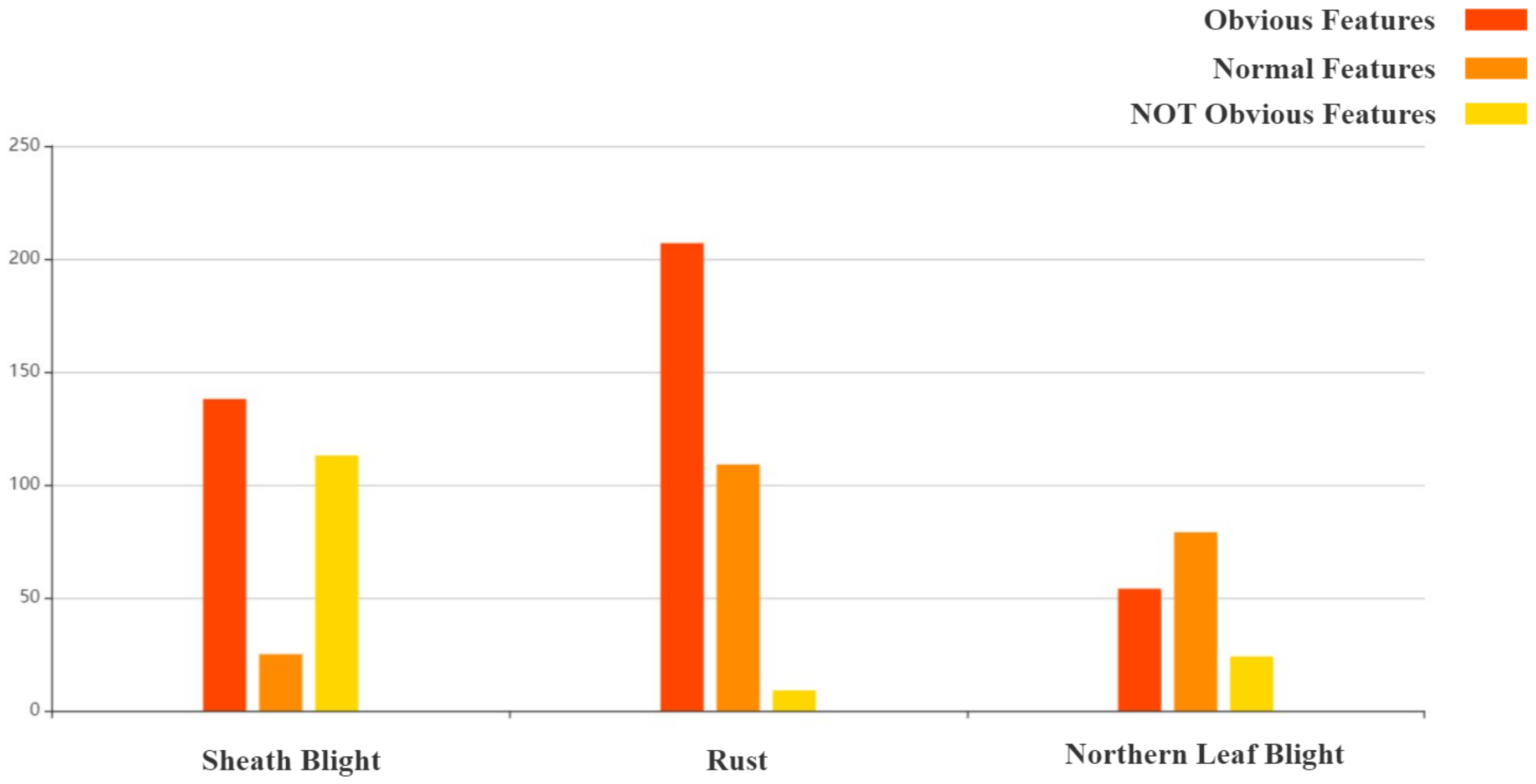
2.1.2. Dataset Analysis

There are several difficulties in the process of data pre-processing, which also brought difficulties to the application of image recognition technology in crop phenotypic analysis: there are often overlapping plants in the image of maize in the densely planted area; the shot will be blurry in windy conditions; the image characteristics of maize leaf diseases vary with the degree of disease; Some of the crops in the data set had more than one disease.

Through further statistical analysis of the dataset, we found that the distribution of the number of lesion features of the three disease images in the dataset sample is shown in Figure 3. About half of each disease image had obvious focal features, and a few had no obvious features. Among the sheath blight disease images, those without obvious lesions account for 40.9%, which will bring challenges to the training of the disease recognition model.

Figure 3. Histogram showing the number of three maize leaf disease images with obvious, normal, and not obvious features.

2.1.3. Data Augmentation

The data augmentation method is usually applied in the case of insufficient training samples. If the sample size of the training set is too small, the training of the network model will be insufficient, or the model will be overfitting. The data amplification method used in this paper includes two parts, simple amplification, and experimental amplification.

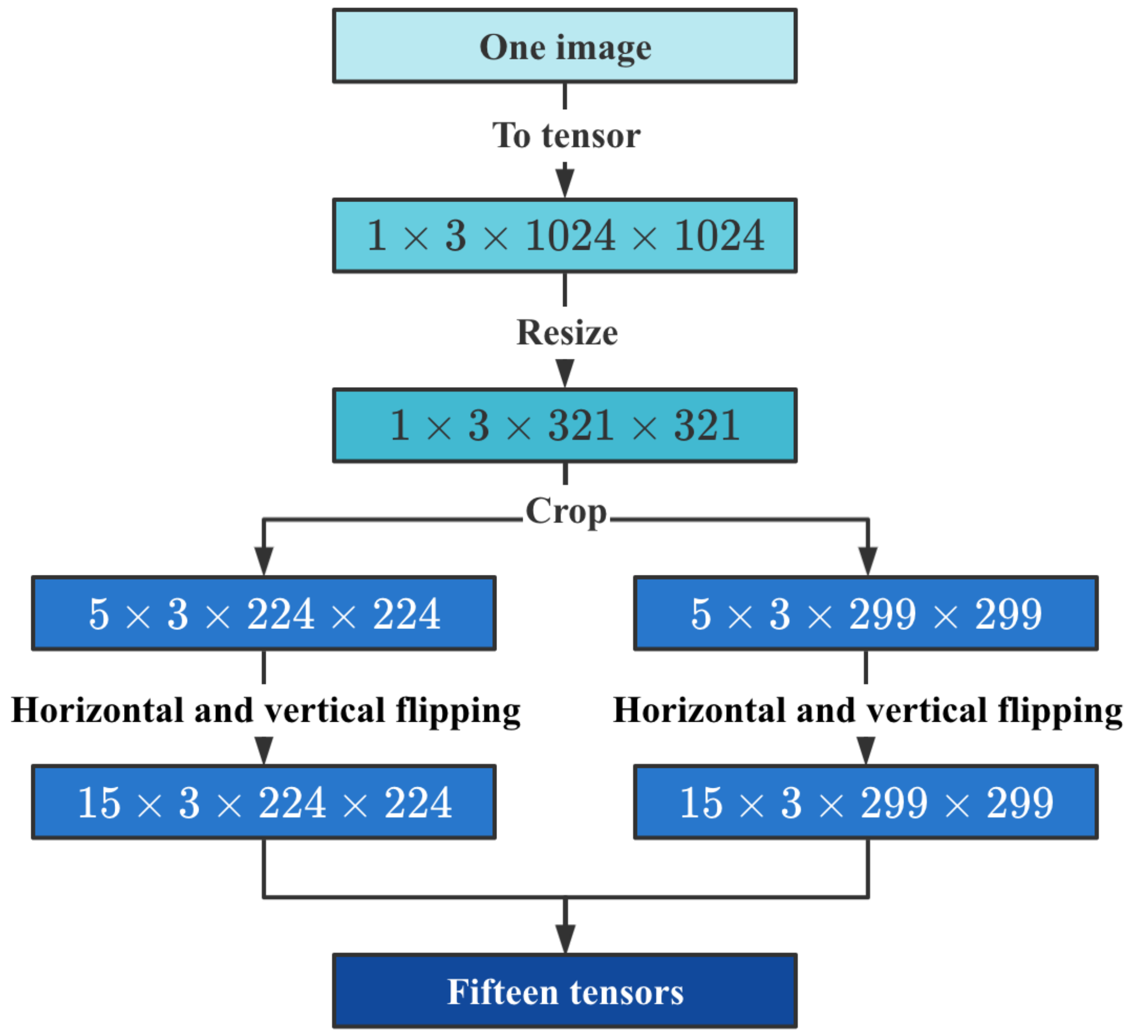
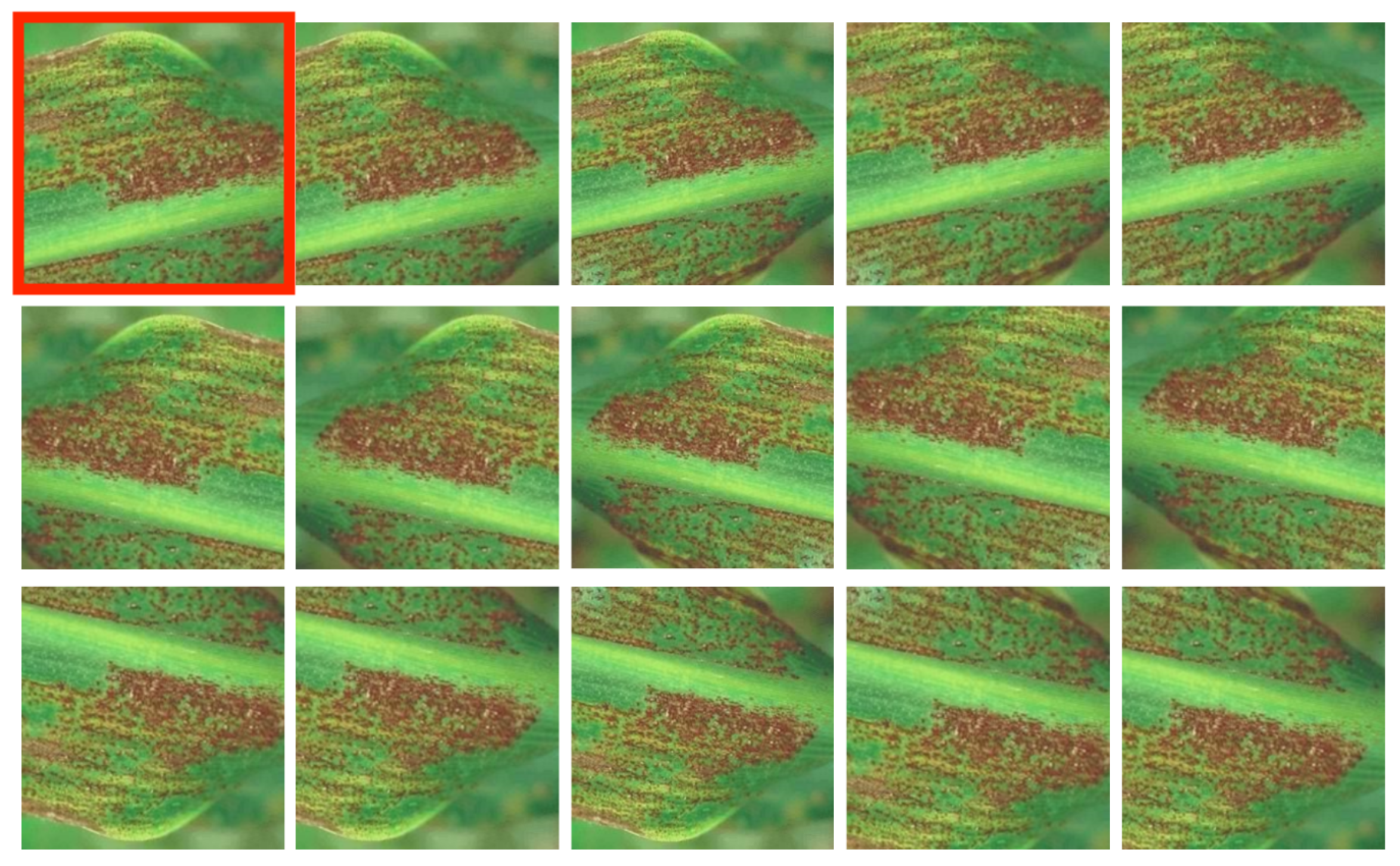
• Simple amplification. We use the traditional image geometry transform, including image translation, rotation, cutting, and other operations. In this study, the method proposed by Alex et al. [8] was explicitly adopted. First, images were cut, the original image was cut into five subgraphs, and then the five subgraphs were flipped horizontally and vertically. Outsourcing frames counted the trimmed training set image to prevent the part of outsourcing frames from being cut out. In this way, each original image will eventually generate 15 extended images and the procedure of data augmentation is illustrated in Figure 4 and Figure 5.
  

  Figure 4. Single image augments to 15 images.
  

  Figure 5. All amplified images corresponding to a single image. First, the image in the red box in the upper left corner is the original image cropped based on the center point. Then the rest four images in the first row are cropped based on the original image’s top left, top right, bottom left, and bottom right. Additionally, images in the second row are horizontally flipped images in the first row. Images in the third row are vertically flipped images in the first row.
• Image graying. The gray-scale processing is a necessary step to preprocess the image, which helps conduct later higher-level operations, such as image segmentation, image recognition, and image analysis [9]
  In this paper, the images involved are expressed in RGB color mode, of which the three RGB components are processed separately in the image procession. However, in disease detection, RGB can only blend colors from the principle of optics but fails to reveal the morphological features of the images.
  Since the visual features of the disease can be retained after gray-scale processing, the number of parameters of the model will be lessened, which can accelerate the training and inferencing process. Specifically, the RGB three-channel images were grayed in the first step. Then the number of parameters in the first convolutional layer of the model was successfully reduced to one third of the original one. Therefore, the training time of the model decreased as a result.
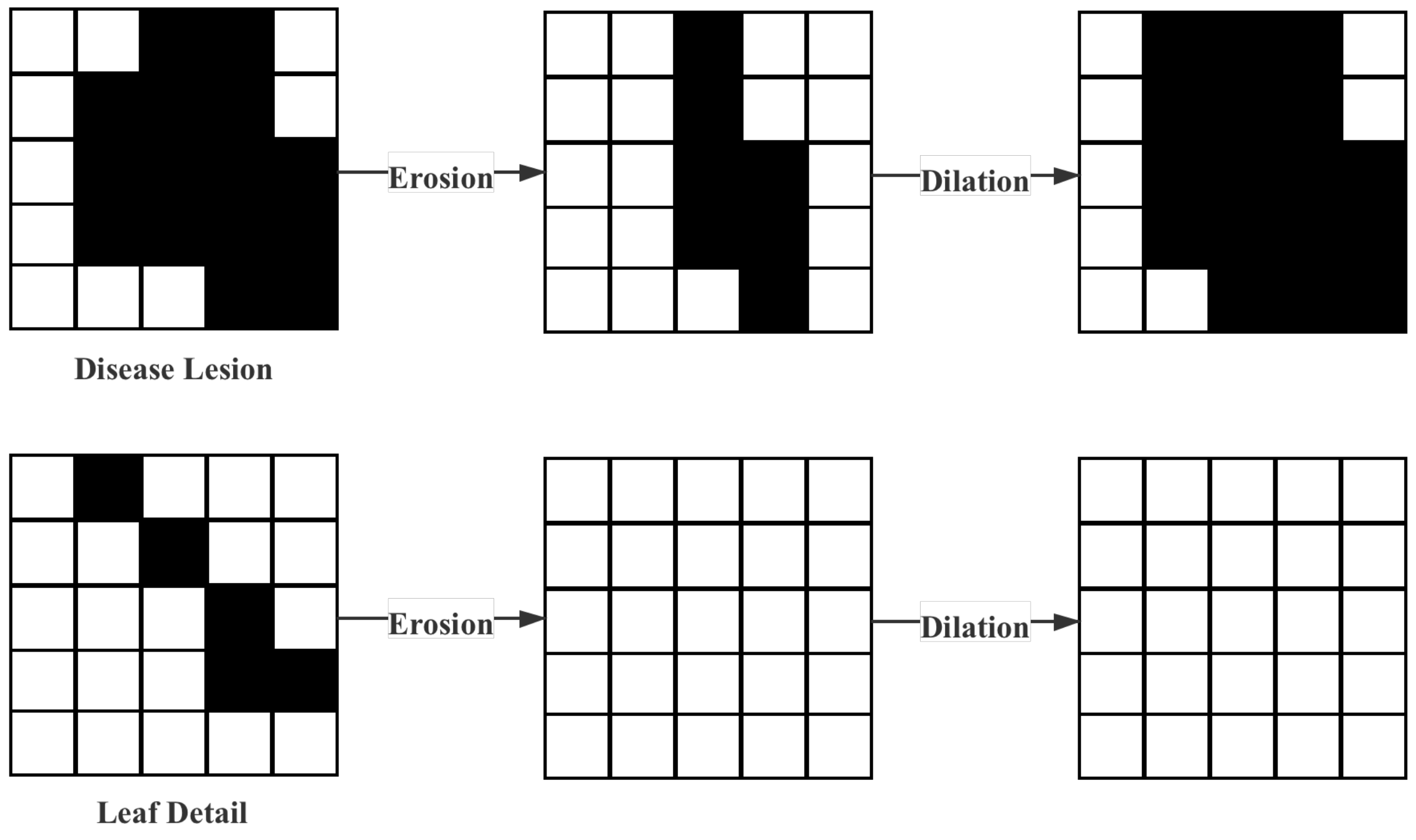
• Removal of interferential leaf details. Given the dataset’s characteristics in this paper, many details in the maize leaf images will interfere with the model, so erosion and dilation [10] were used to preprocess the data. First, the erosion operation is performed. The logical operation process is shown in Equation (1). The leaf details can be removed through the erosion operation, but this operation would also change the characteristics of the lesion. Therefore, the dilation process was necessary, and the logical operation process is shown in Equation (2). In Equations (1) and (2), A represents the original image, and B represents the operator. The original characteristics of the lesion can be restored through the expansion process. The operation process above is shown in Figure 6.

  $$A\odot B=\left\{z\right|{\left(\widehat{B}\right)}_z\subseteq A\}$$

  (1)

  $$A\oplus B=\left\{z\right|{\left(\widehat{B}\right)}_z\cap A\ne \varnothing \}$$

  (2)
  

  Figure 6. Processing of removal of interferential leaf details.
• Snapmix and Mosaic. Currently, popular data amplification methods in deep learning research include Snapmix [11] and Mosaic [12]. In this study, these two methods were used for further data amplification based on 59,778 training samples. Different amplification methods were used to evaluate the comparative experimental results. The Snapmix method randomly cuts out some areas in the sample and fills them with a particular patch from other images stochastically and the classification label remains unchanged. The mosaic method could use multiple pictures at once, and its most significant advantage lies in the fact that it could enrich the background of the detected objects.
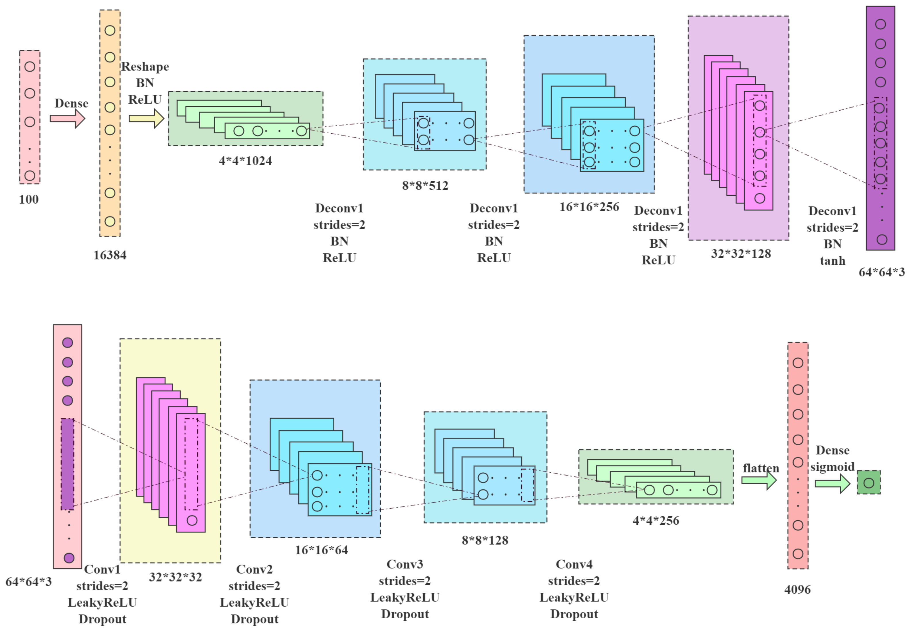
• In this paper, the generation of synthetic data plays a vital role in model training. As for the missing data, many measures have been proposed to tackle these problems. Suppose there is a limitation on the training data. In that case, it is necessary to generate three kinds of data, i.e., three disease images of maize leave sick with sheath blight, rust, and northern leaf blight. A Gaussian-based sampling method will be adopted to generate imagers based on available images. The two required parameters include the mean and standard deviation. The probability density distribution of the Gaussian distribution is displayed as Equation (3):

  $$p\left(x\right)=\frac{1}{\sqrt{2\pi }\sigma }{e}^{-\frac{{(x-\mu )}^2}{2{\sigma }^2}}$$

  (3)
  The x is the eigenvector. After varying the mean and standard deviation, the desired eigenvectors of disease images will be generated based on the samples from the normal Gaussian distribution.
  Given the available eigenvectors which correspond to the normal and diseased leaves, a synthetic data generator based on DCGAN [13] is established. The generator plays the role of generating much more available feature vectors of normal and diseased leaves, and in turn, enriching the training step in reinforcement learning. In the DCGAN, there are two participants: the generator G and the discriminator D. Let $p_{d}ata$ denote the distribution of feature vectors extracted from them. The aim of the generator model G lies in generating probability distribution on the feature vector data. Commonly, two deep neural networks are designed to represent the generator and discriminator. The optimized objective of the DCGAN model can be mathematically expressed in Equation (4):

  $$\underset{G}{min}\underset{D}{max}V(D,G)={\mathbb{E}}_{\left(x\sim p_{\mathrm{data}}\right)}[logD\left(x\right)]+{\mathbb{E}}_{\left(z\sim p_{z\left(z\right)}\right)}[log(1-D\left(G\left(z\right)\right))]$$

  (4)
  The structure of DCGAN is shown in Figure 7.
  

  Figure 7. Structure of DCGAN.

As a result, the data set will be expanded from 4428 image samples to 89,420 data samples, and the result of data augmentation is shown in Table 1.

Table 1. Distribution of dataset.

	Normal	Sheath Blight	Rust	Northern Leaf Blight	Total
Original data set	2735	521	459	713	4428
After data augmentation	41,025	17,815	16,885	13,695	89,420
Training set	36,923	16,034	15,197	12,326	80,478
Validation set	4102	1781	1688	1369	8942

2.1.4. Image Quality Assessment

In this section, PSNR and SSIM [14] indexes are used to evaluate the quality of amplified images. The specific results are shown in Table 2.

Table 2. Comparison of quantitative results of different algorithms.

Index	DCGAN	Snapmix	Mosaic
PSNR	27.9 dB	16.8 dB	15.3 dB
SSIM	0.818	0.438	0.411

2.2. Multi-Activation Function Module

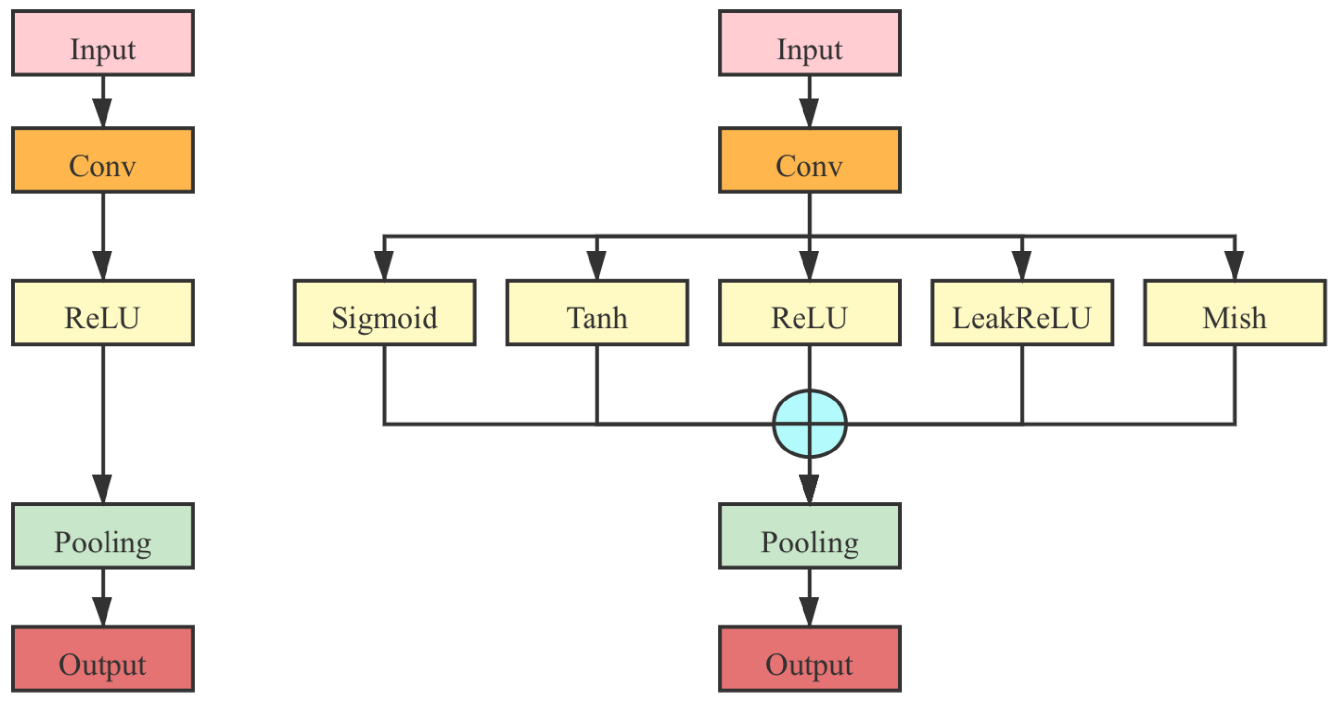
2.2.1. Combination of Different Activation Functions

In the network structure of a single activation function, the input x is passed into the convolution layer, the batch normalization layer, and the activation function layer obtains the output. The MAF module means that when x is output from the batch normalization layer, it will be divided into multiple pathways. Each branch is activated by different activation functions and then fused. The rule of fusion of multiple activation functions is displayed in Equation (5).

$$x_{w,h,c}=\sum _{i=1}^k{w}^k{f}_{\left(x_{w,h,c}\right)}^k$$

(5)

A weight $w^k$ is given for each branch, and the $softmax$ function processes the weights to ensure a probability sum.

Since the MAF module contains the ReLU function and the weight $w^k$ in the MAF participates in updating the backpropagation algorithm, the sum of weights is always 1. It can be theoretically proven that the result of the optimized network cannot be worse than the original networks in terms of performance. When the non-ReLU activation function weights are 0, the MAF module is degraded to a one-pathway ReLU activation function layer.

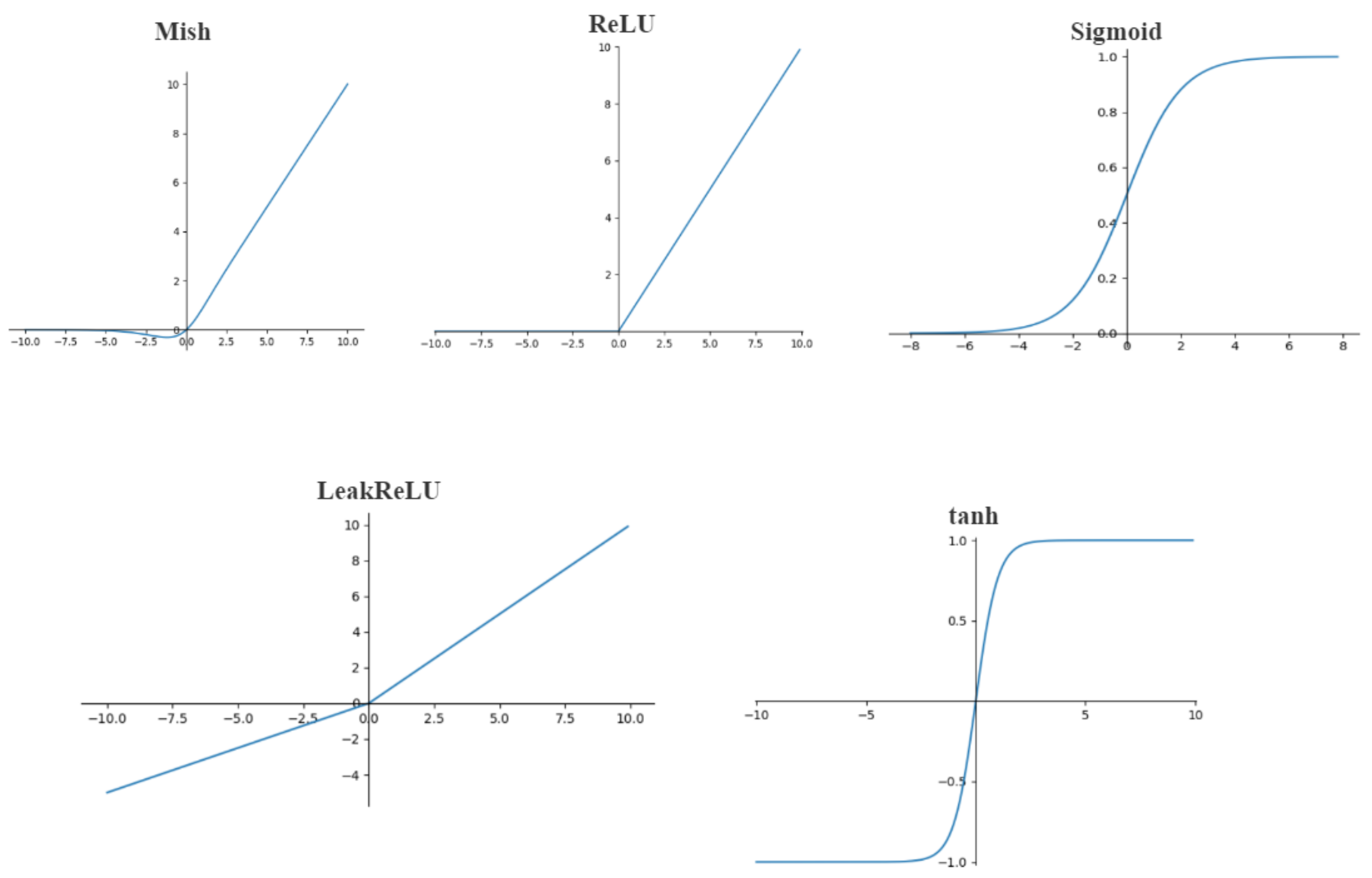
2.2.2. Base Activation Functions

• Mish [15], as shown in Figure 8, is an activation function designed to replace ReLU proposed by Diganta Misra. It was claimed that it broke a part of the previous accuracy score record on the FastAI global leaderboard. Its mathematical expression is: $y=x\times tanh\left(ln(1+e^x)\right)$.
  

  Figure 8. Base activation functions.
• ReLU function is adopted by the activation function used in many of the backbone networks mentioned above by default, and was first applied to the AlexNet.
• LeakReLU is an activation function, where the leak is a tiny constant so that some values of the negative axis are preserved, and not all information of the negative axis is lost.
• Tanh is one of the hyperbolic functions. In mathematics, the hyperbolic tangent is derived from the hyperbolic sine and hyperbolic cosine of the fundamental hyperbolic function. Its mathematical expression is $tanh\left(x\right)=\frac{sinh\left(x\right)}{cosh\left(x\right)}=\frac{e^x-e^{-x}}{e^x+e^{-x}}$.
• Sigmoid is a smooth step function that can be derived. Sigmoid can convert any value to $[0,1]$ probability and is mainly used in binary classification problems. The mathematical expression is $y=\frac{1}{1+e^{-x}}$.

2.2.3. Apply MAF Module to Different CNNs

CNNs have been developed over the years. Different model structures are generated and divided into three types: (1) AlexNet [8] and VGG [16], which form a network structure by repeatedly stacking convolutional layers, activation function layers and pooling layers; (2) ResNet [17] and DenseNet [18], residual networks; (3) GoogLeNet [19], a multi-pathway parallel network structure. To verify the effectiveness of the MAF module, it is integrated into different networks at different levels.

• In the AlexNet and VGG series, as shown in Figure 9, the activation function layer is directly replaced with the MAF module in the original networks.
  

  Figure 9. MAF module applied to the VGG series (the original one is on the left; the optimized one is on the right).
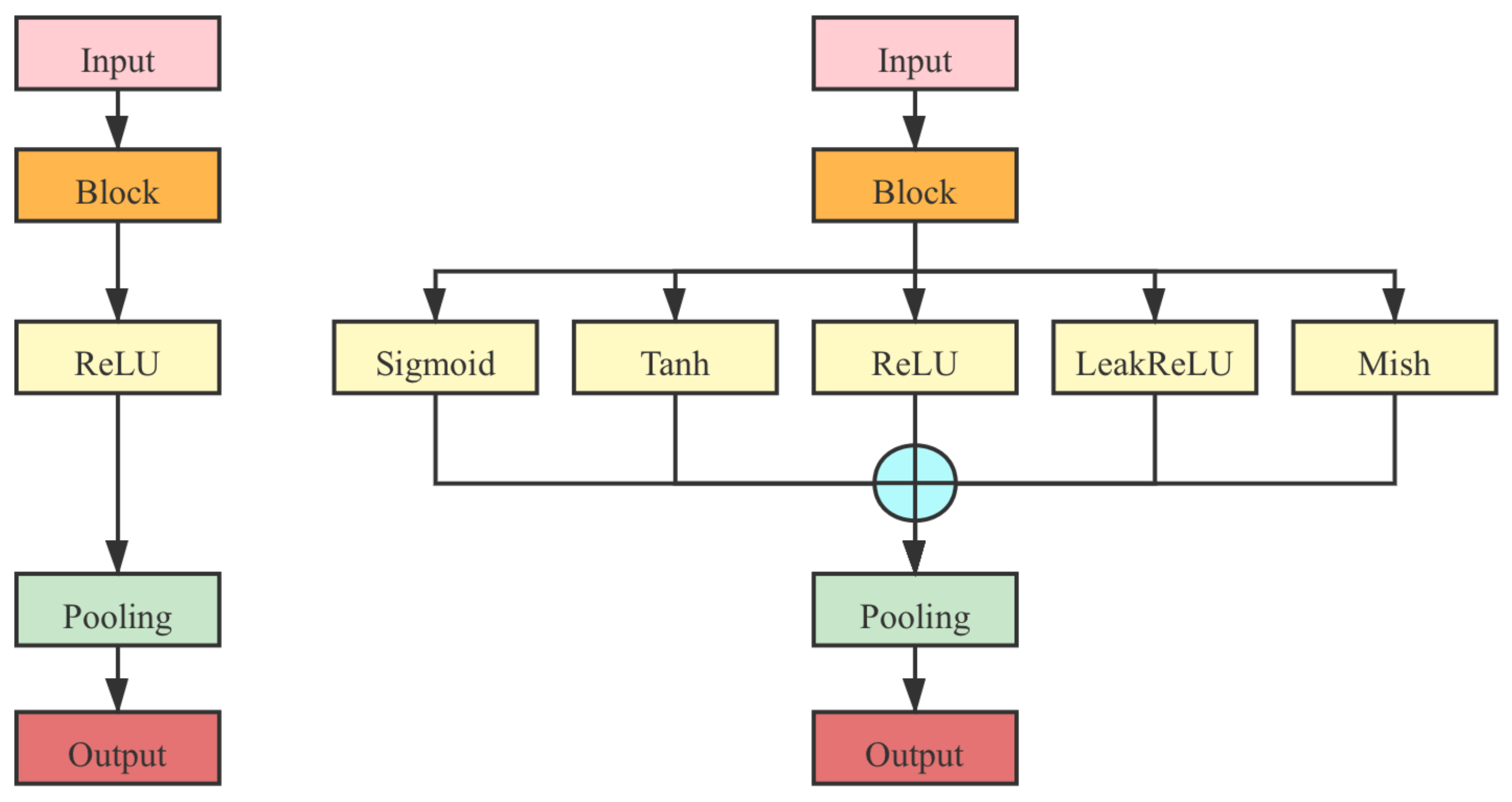
• In the ResNet series, as shown in Figure 10, the ReLU activation function layer is replaced between the block with an MAF module.
  

  Figure 10. MAF module applied to the ResNet series (the original one is on the left; the optimized one is on the right).
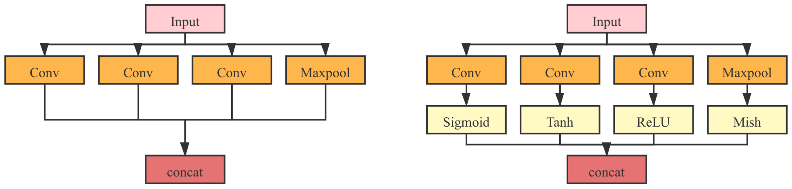
• In the GoogLeNet, as shown in Figure 11, an MAF module was applied inside the inception module. Diverse activation functions were applied to the branches inside the inception accordingly.
  

  Figure 11. MAF module applied to the GoogLeNet (the original one is on the left; the optimized one is on the right).

3. Results

3.1. Experiment

The experiment is based on the PyTorch framework. The processor is Intel (R) Core (TM) i9. The memory is 16 GB, and the graphics card is NVIDIA GeForce RTX3080 10 GB.

Since each model of the VGG series, ResNet series, and DenseNet series contained many sub-models. Moreover, the subsequent experiments to test the accuracy of different activation function combinations, which consisted of different sub-models and different functions, were too complicated. Consequently, benchmarks were performed on all sub-models of these three networks. The experimental results are shown in Figure 12, Figure 13 and Figure 14. It could be concluded that VGG19, ResNet50, and DenseNet161 performed best among the three network models. Thus, subsequent experiments would adopt these three sub-models to test the self-network models.

Figure 12. Experiment results of VGGNet series.

Figure 13. Experiment results of ResNet series.

Figure 14. Experiment results of DenseNet series.

3.1.1. Training Strategy

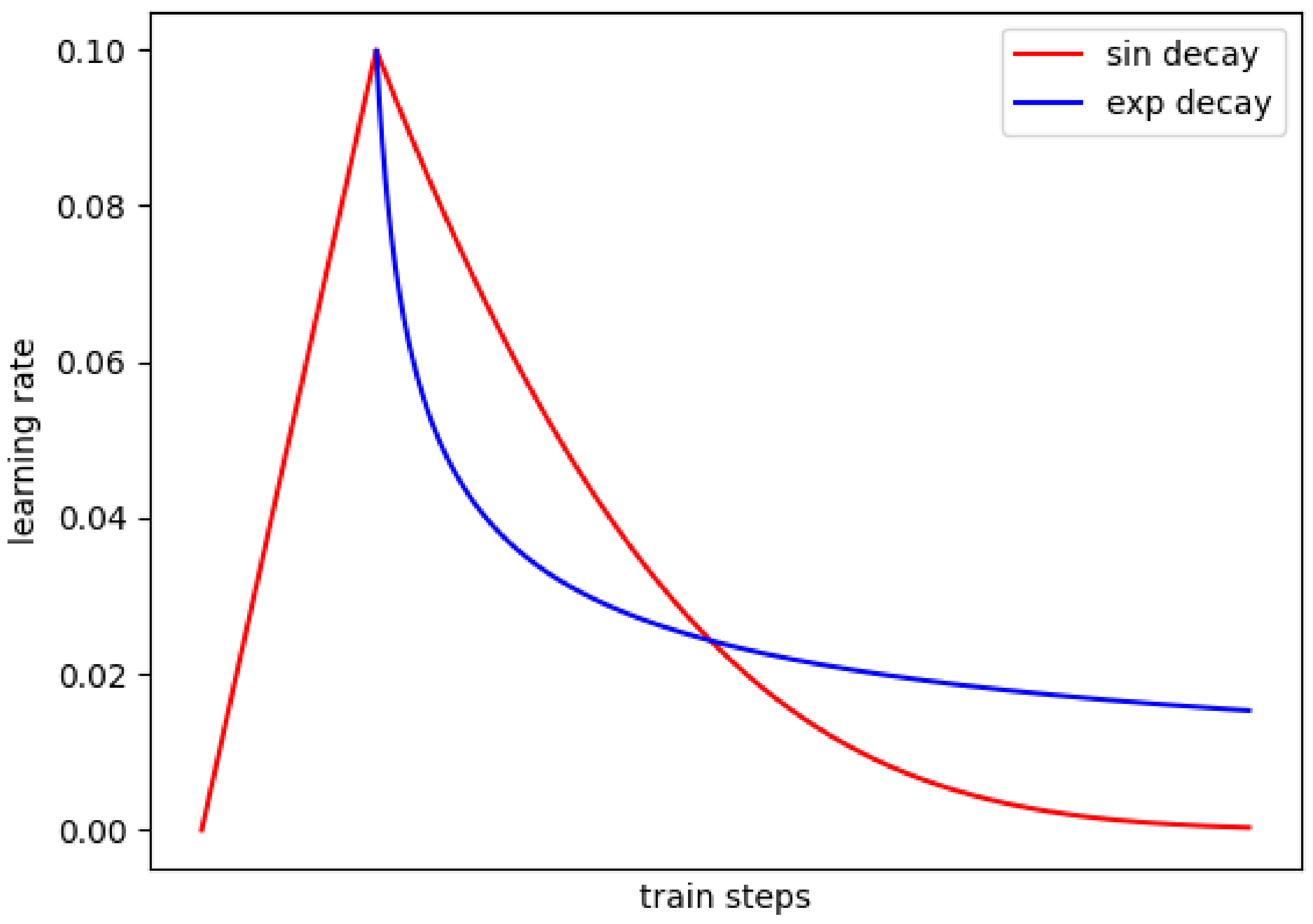
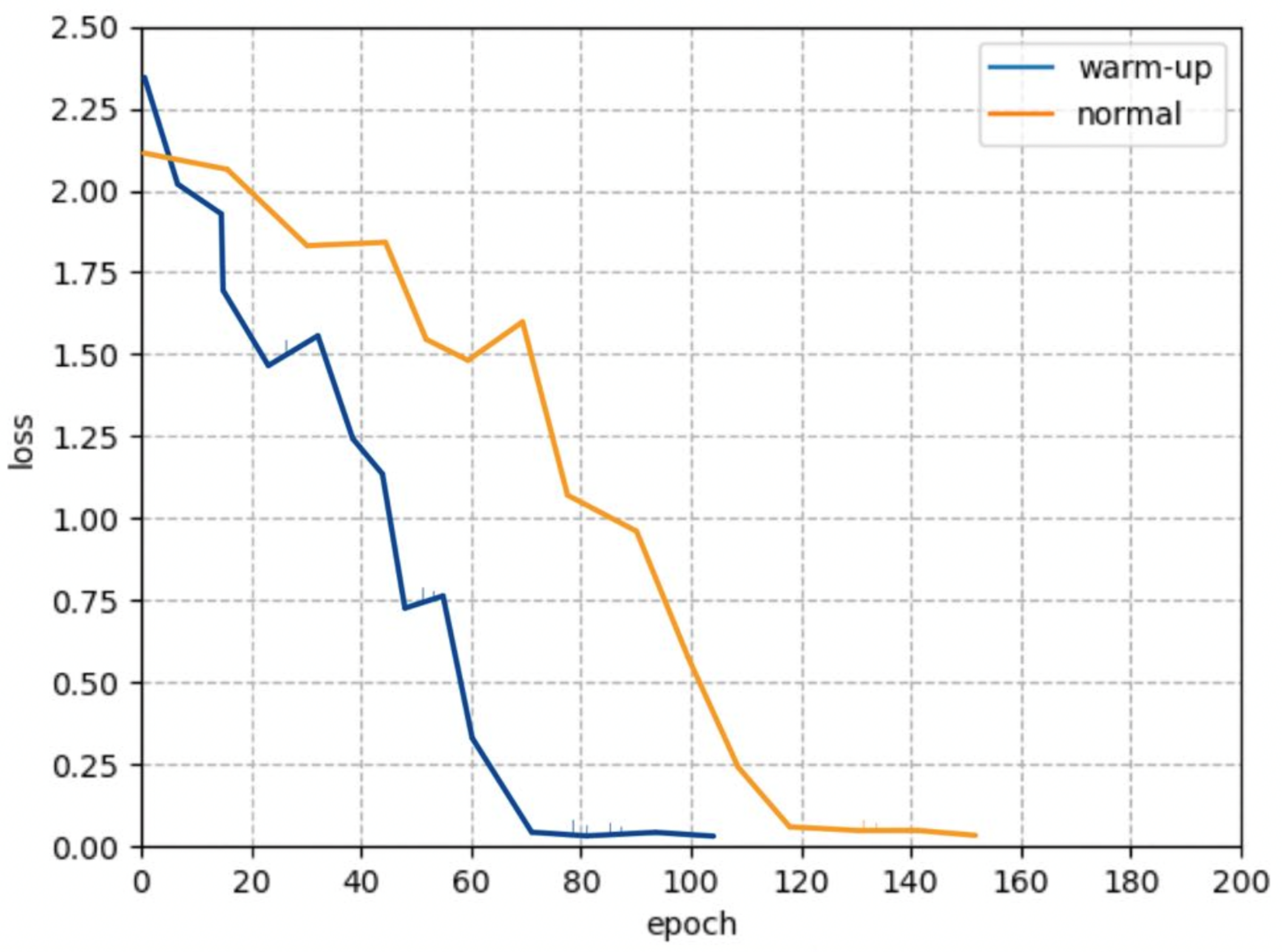
The pre-training model parameters used in this paper are provided by PyTorch based on the ImageNet dataset. ImageNet is a classification problem that demands to divide the images into 1000 classifications. The number of the parameters of network’s last fully connected layer is 1000, which needs to be modified to four in this paper.

The first convolutional layer is reduced to one third of the original number of parameters, and the last fully connected layer is reduced to one-250th of the original number of parameters. In this paper, the initialization method is the Kaiming initialization method proposed by Kaiming [20]. This method is well suited for the non-saturated activation function ReLU and its variant types.

In this paper, the samples were divided into training and validation sets according to 9:1, The loss function optimization strategy used for training was SGD (stochastic gradient descent) [21], where the momentum parameter was set as 0.9, and the batch size parameter was set as 50. After 50 iterations, the accuracy of the validation set tended to converge. Further training will lead to a decrease in the accuracy of the validation set and overfitting. Thus, the model parameters were selected as the model parameters trained after 200 iterations.

3.1.2. Warm-Up

Warm-up [17] is a training idea. In the pre-training phase, a small learning rate is first used to train some steps, and then modified to a preset learning rate for training. When the training begins, the model’s weights are randomly initialized, and the “understanding level” of the data is 0. The model may oscillate if a more extensive learning rate is used at the beginning. In preheating, training is performed with a low learning rate, so that the model has specific prior knowledge of the data, and then a preset learning rate is used for training so that the model convergence speed will be faster, and the effect can be better. Finally, a small learning rate to continue the exploration can avoid missing local optimal points. For example, during the training process, set the learning rate as 0.01 to train the model until the error is less than 80%. In addition, then set the learning rate as 0.1 to train.

The warm-up mentioned above is the constant warm-up. There may be an unexpected increase in training errors when changing from a small learning rate to a relatively large one. So in 2018, Facebook came up with a step-by-step warm-up approach to solve the problem, starting with a small initial learning rate and increasing it slightly with each step until the initial setting reached a relatively large learning rate, then it is adopted for training.

$exp$ warm-up was tested in this paper, i.e., the learning rate increases linearly from a small value to a preset learning rate, and then decays according to $exp$ function law. At the same time, the $sin$ warm-up is tested, the learning rate increases linearly from a tiny value and decays after reaching a preset value according to the $sin$ function law. For the two pre-training methods, the changes are shown in Figure 15.

Figure 15. Warmup Learning Rate Schedule.

3.1.3. Label-Smoothing

In this paper, the backbone network would output a confidence score that the current data corresponded to the foreground. The softmax function normalize these scores, as a result, the probability of each current data category could be obtained. The calculation is shown in Equation (6).

$$q_i=\frac{exp\left(z_i\right)}{{\sum }_{j=1}^K{p}_{i}log{q}_i}$$

(6)

Then calculate the cross-entropy cost function, as shown in Equation (7).

$$Loss=-\sum _{i=1}^K{p}_{i}log{q}_i$$

(7)

Among it, the calculation method of $p_i$ is shown in Equation (8).

$$p_i=\left\{\begin{array}{c}\hfill 1,if(i=y)\\ \hfill 0,if(i\ne y)\end{array}\right.$$

(8)

For the loss function, the predicted probability should be adopted to fit the true probability. However, two problems will occur after fitting the one-hot true probability function: the model’s generalization ability could not be guaranteed, and it is likely to result in overfitting. The gap between classifications tends to be as large as possible due to the total probability and 0 probability. Moreover, the bounded gradient indicated that it was challenging to adapt to this situation. It would lead to the result that the model trusted the predicted category too much. Especially when the training dataset was small, it was not enough to represent all sample features, which was helpful for the overfitting of the network model.

Based on this, the regularization strategy of label-smoothing [22] was used to solve problems mentioned above, adding noise through a soft one-hot, reducing the weight of the real sample label classification in the calculation of the loss function, and finally helping suppress overfitting.

After adding the label-smoothing, the probability distribution changed from Equation (8) to Equation (9).

$$p_i=\left\{\begin{array}{c}\hfill 1-ϵ,if(i=y)\\ \hfill \frac{ϵ}{K-1},if(i\ne y)\end{array}\right.$$

(9)

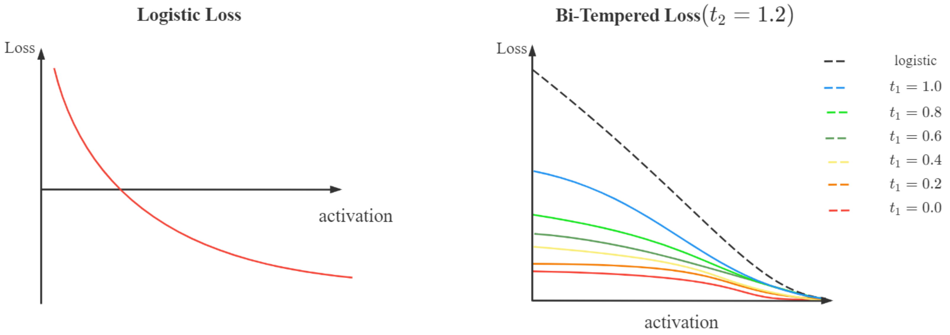
3.1.4. Bi-Tempered Logistic Loss

The original CNN’s loss function of image classification was the logistic loss function, but it possessed two drawbacks. In the dataset, the number of diseased samples was quite insufficient and likely to contain noise, which was to blame for shortcomings when the logistic loss function processed these data. The disadvantages were as follows:

• In the left-side part, close to the origin, the curve was steep, and there was no upper bound. The label samples that were incorrectly marked would often be close to the left y-axis. The loss value would become very large under this circumstance, which leads to an abnormally large error value that stretches the decision boundary. In turn, it adversely affects the training result, and sacrifices the contribution of other correct samples as well. That was, far-away outliers would dominate the overall loss.
• As for the classification problem, $softmax$, which expressed the activation value as the probability of each class, was adopted. If the output value were close to 0, it would decay quickly. Ultimately the tail of the final loss function would also exponentially decline. The unobvious wrong label sample would be close to this point. Meanwhile, the decision boundary would be close to the wrong sample because the contribution of the positive sample was tiny, and the wrong sample was used to make up for it. That was, the influence of the wrong label would extend to the boundary of the classification.

This paper adopted the Bi-Tempered loss [23] to replace Logistic loss to cope with the question above. From Figure 16, it could be concluded that both types of loss could produce good decision boundaries with the absence of noise, thus successfully separating these two classes. In the case of slight margin noise, the noise data were close to the decision boundary. It could be seen that due to the rapid decay of the $softmax$ tail, the logic loss would stretch the boundary closer to the noise point to compensate for their low probability. The bistable loss function has a heavier tail, keeping the boundary away from noise samples. Due to the boundedness of the bistable loss function, when the noise data were far away from the decision boundary, the decision boundary could be prevented from being pulled by these noise points.

Figure 16. Logistic loss and Bi-Tempered loss curves.

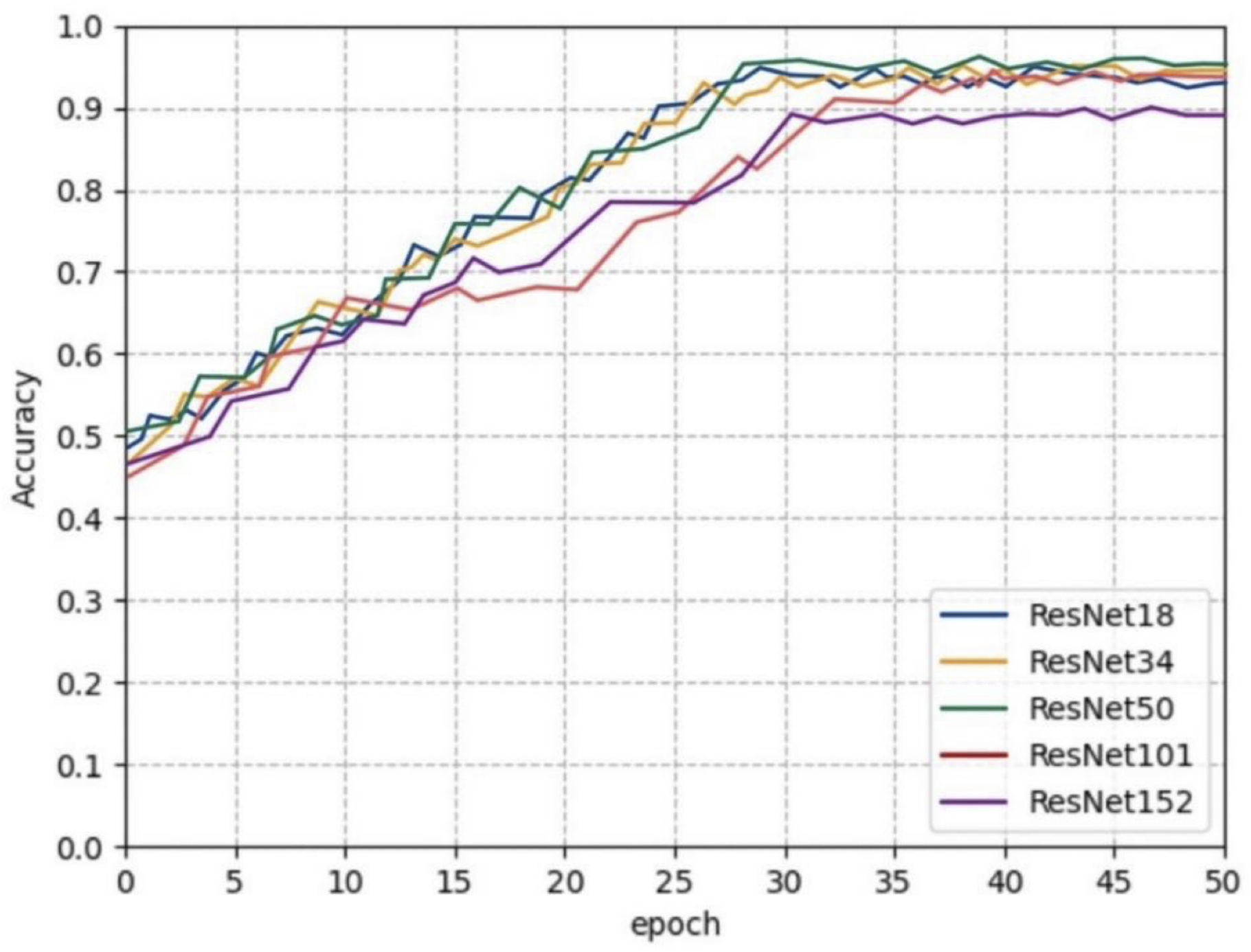
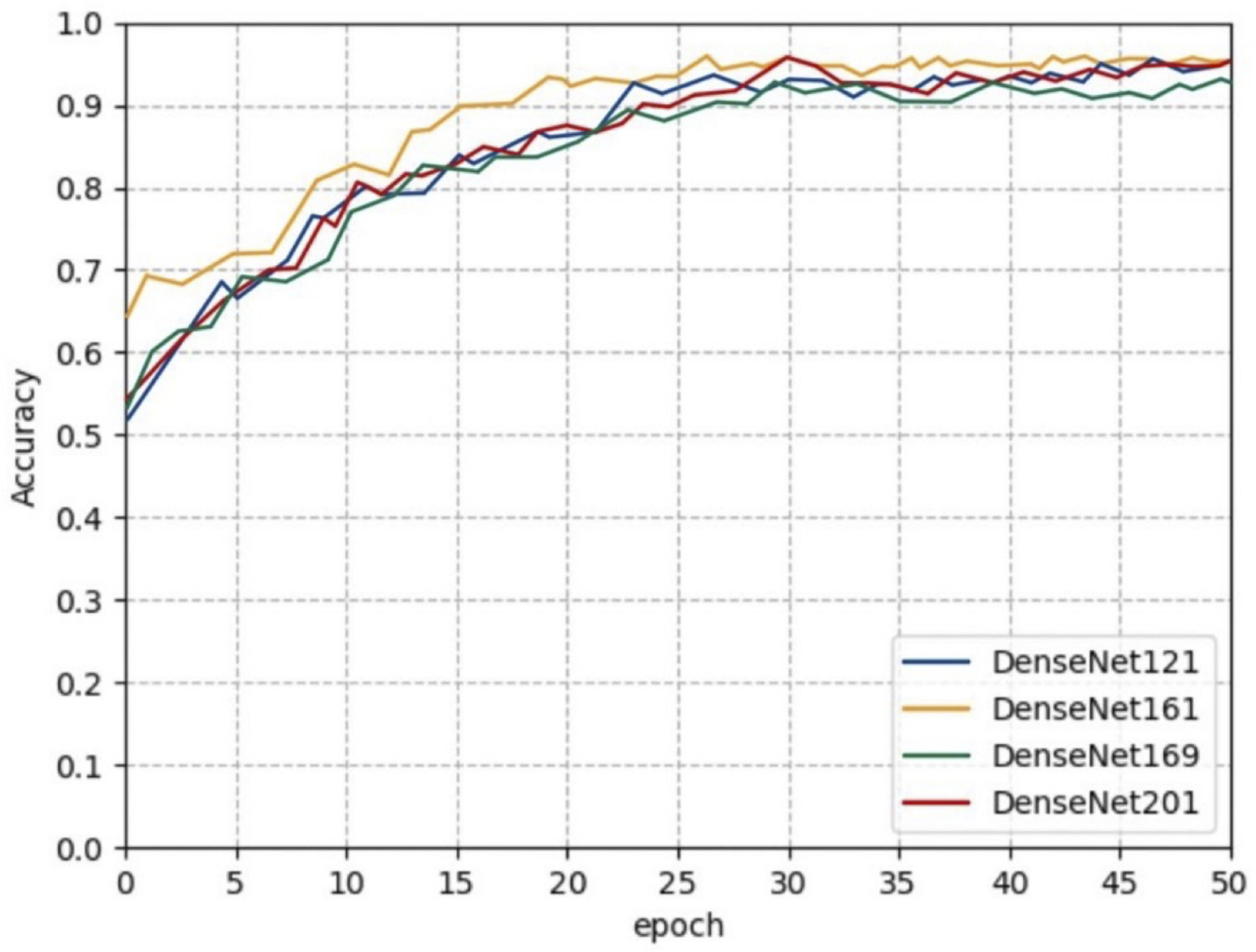
3.2. Experiment Results

This paper demonstrates the outstanding performance of CNNs in maize leaf disease detection by comparing the accuracy of plenty of CNNs, including AlexNet, VGG19, ResNet50, DenseNet161, GoogLeNet, and their optimized versions based on MAF module, with traditional machine learning algorithms, SVM [24] and RF [25]. The comparison results are shown in Table 3.

Table 3. Accuracy of different models.

Model	Tanh	ReLU	LeakyReLU	Sigmoid	Mish	Accuracy
SVM						83.18%
RF						87.13%
baseline						92.82%
	🗸	🗸	🗸	🗸	🗸	93.11%
MAF-AlexNet	🗸		🗸	🗸		93.49%
		🗸	🗸	🗸		92.80%
baseline						93.92%
	🗸	🗸	🗸	🗸	🗸	94.93%
MAF-VGG19		🗸		🗸	🗸	95.30%
	🗸			🗸	🗸	95.18%
baseline						95.08%
	🗸	🗸	🗸	🗸	🗸	95.93%
MAF-ResNet50	🗸	🗸		🗸		97.41%
			🗸	🗸	🗸	96.18%
baseline						96.18%
	🗸		🗸	🗸		95.90%
MAF-DenseNet161	🗸			🗸	🗸	96.75%
	🗸	🗸		🗸		97.01%
baseline						94.27%
MAF-GoogLeNet	🗸	🗸	🗸	🗸	🗸	95.01%
	🗸		🗸	🗸		95.09%
	🗸		🗸	🗸		94.27%

The results of experiments indicate that the accuracy of the mainstream CNNs could be improved with the MAF module, and the effect on the ResNet50 stands out, reaching 2.33%. In addition, it is also found that the promoting effect of adding all activation functions to the MAF module is not the best. Instead, the combination of Sigmoid, ReLU (or tanh), and Mish (or LeakReLU) ranks top.

3.2.1. Ablation Experiments to Verify the Effectiveness of Warm-Up

Ablation experiments were performed on multiple models to verify the validation of the warm-up method. The results are shown in Figure 17.

Figure 17. Loss curve of different models and methods.

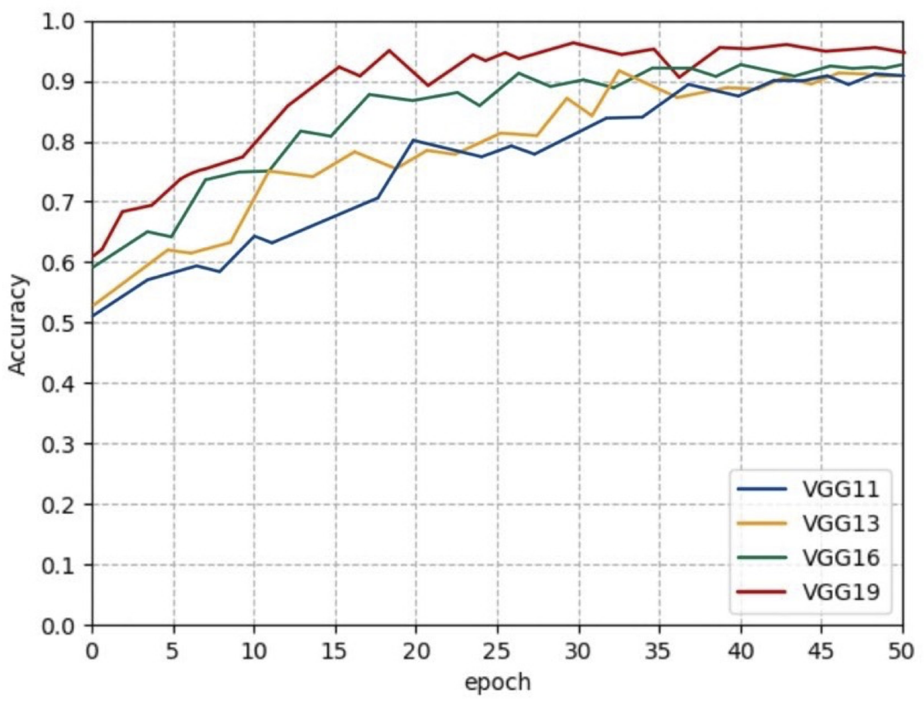
3.2.2. Ablation Experiments

To verify the effectiveness of the various pre-processing techniques proposed in this article, such as different data augmentation methods, the ablation experiments were performed on MAF-ResNet50, selected from the above experiments with the best performance. The experimental results are shown in Table 4 and Table 5.

Table 4. Ablation experiment result of different pre-processing methods.

	Removal of Details	Gray-Scale	Snapmix	Mosaic	Accuracy
baseline					95.08%
MAF-ResNet50	🗸	🗸	🗸	🗸	97.41%
	🗸	🗸	🗸		96.29%
	🗸	🗸		🗸	95.82%
	🗸		🗸	🗸	93.17%
		🗸	🗸	🗸	94.39%

Table 5. Ablation experiment result of other methods.

	DCGAN	Label-Smoothing	Bi-Tempered Loss	Accuracy
baseline				95.08%
MAF-ResNet50	🗸	🗸	🗸	96.53%
	🗸	🗸		97.41%
	🗸		🗸	95.77%
		🗸	🗸	97.22%

Through the analysis of experimental results, we can find those data enhancement methods such as Snapmix and Mosaic are of great assistance in improving the performance of the MAF-ResNet50 model. The principles of Snapmix and Mosaic are similar. It could be seen that the model performs best when warm-up, label-smoothing, and Bi-Tempered logistic loss methods are used simultaneously, as shown in Table 5.

4. Discussion

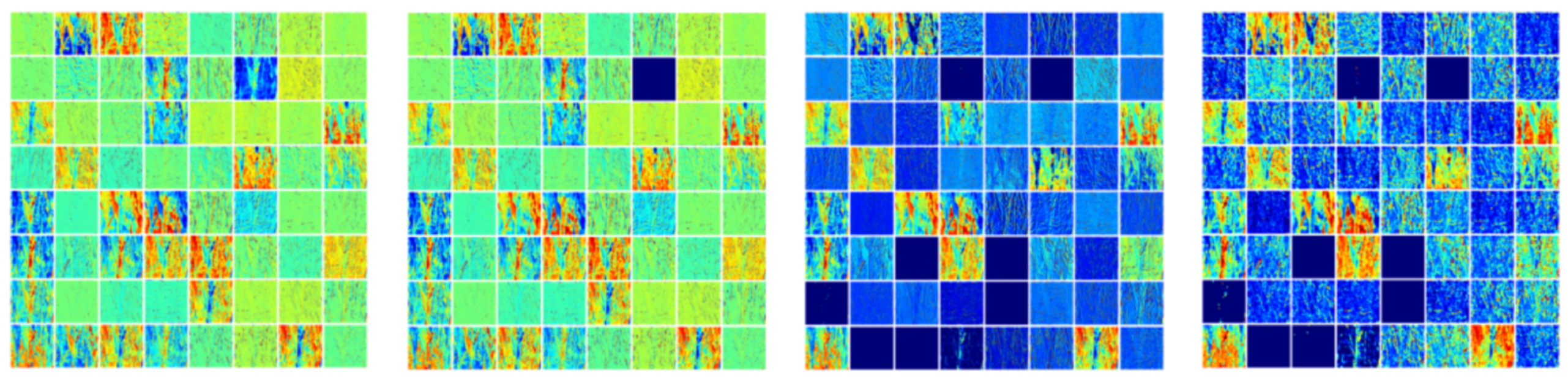
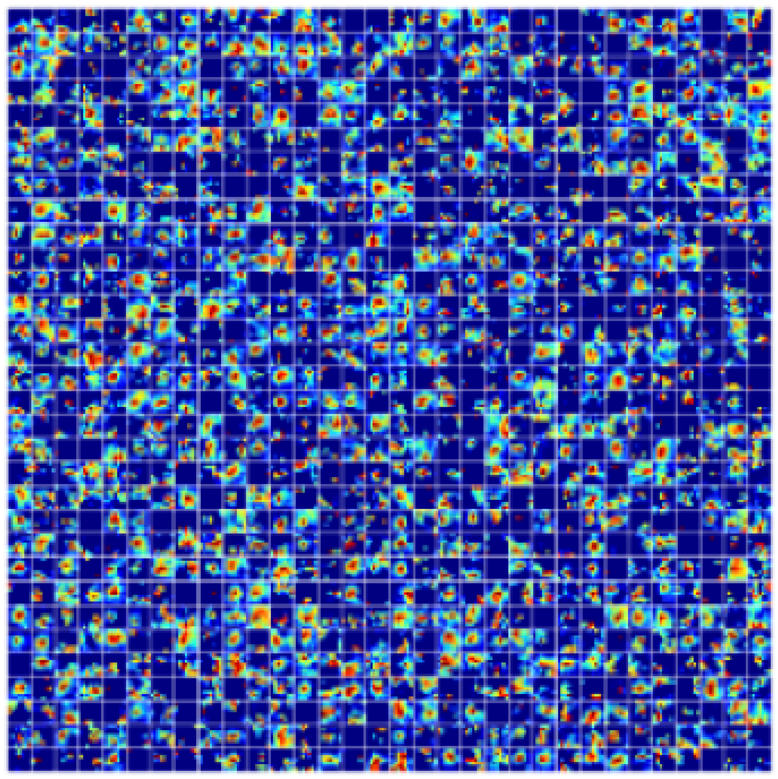
4.1. Visualization of Feature Maps

In this paper, the output of multi-channel feature graphs corresponding to eight convolutional layers of the MAF-ResNet50 was visualized with the highest accuracy in the experiment, as shown in Figure 18. As can be seen from the figure, in the shallow layer feature map, MAF-ResNet50 extracted the lesion information of the maize stalk lesion and carried out depth extraction in the subsequent feature map. As the network layer deepened, the interpretability of the feature map visualization became worse. Nevertheless, even in Figure 19, the corresponding relationship between the highlighted color block area of the feature map and the lesion area in the original image can still be observed, which further reveals the effectiveness of the MAF-ResNet50 model.

Figure 18. Visualization of shallow feature maps.

Figure 19. Visualization of the deep feature map.

4.2. Intelligent Detection System for Maize Diseases

To verify the robustness of the MAF module proposed in this paper, we also used the data set collected from the Science Park in the west campus of China Agriculture University, including the images of maize diseases such as southern leaf blight, fusarium head blight, and those three kinds mentioned above. Additionally, we developed the mobile detection device based on the iOS platform, which won the second prize in The National Computer Design Competition for Chinese College Students. As shown in Figure 20, the optimized model based on the proposed method can quickly and effectively detect maize diseases in practical application scenarios, proving the proposed model’s robustness.

Figure 20. Screenshot of launch page and detection pages.

5. Conclusions

This paper proposed an MAF module to optimize mainstream CNNs and gained excellent results in detecting maize leaf diseases with the accuracy reaching 97.41% on MAF-ResNet50. Compared with the original network model, the accuracy improved by 2.33%. Since the CNN was unstable, non-convergent and overfitting when the image set was insufficient, multiple image pre-processing methods, meanwhile, models were applied to extend and augment the data of disease samples, such as DCGAN. Transfer learning and warm-up methods were adopted to accelerate the training speed of the model.

To verify the effectiveness of the proposed method, this paper applied this model to multiple mainstream CNNs; the results indicated that the performance of networks adding the MAF module have all been improved. Afterward, this paper discussed the performance of different combinations of five base activation functions. Based on a large number of experiments, the combination of Sigmoid, ReLU (or tanh), and Mish (or LeakReLU) reached the highest rate of accuracy, which was 97.41%. The result proved the effectiveness of the MAF module, and the improvement is of considerable significance to agricultural production. The optimized module proposed in this paper can be well applied to numerous CNNs.

In the future, the author will make efforts to replace the combination of linear activation functions with that of nonlinear activation functions and make more network parameters participate in model training.

References

- Yu, J.; Wang, J.; Leblon, B. Evaluation of Soil Properties, Topographic Metrics, Plant Height, and Unmanned Aerial Vehicle Multispectral Imagery Using Machine Learning Methods to Estimate Canopy Nitrogen Weight in Corn. Remote Sens. 2021, 13, 3105. [Google Scholar] [CrossRef]
- Xie, Q.; Wang, J.; Lopez-Sanchez, J.M.; Peng, X.; Liao, C.; Shang, J.; Zhu, J.; Fu, H.; Ballester-Berman, J.D. Crop height estimation of corn from multi-year RADARSAT-2 polarimetric observables using machine learning. Remote Sens. 2021, 13, 392. [Google Scholar] [CrossRef]
- Lee, H.; Wang, J.; Leblon, B. Using linear regression, Random Forests, and Support Vector Machine with unmanned aerial vehicle multispectral images to predict canopy nitrogen weight in corn. Remote Sens. 2020, 12, 2071. [Google Scholar] [CrossRef]
- Kayad, A.; Sozzi, M.; Gatto, S.; Marinello, F.; Pirotti, F. Monitoring within-field variability of corn yield using Sentinel-2 and machine learning techniques. Remote Sens. 2019, 11, 2873. [Google Scholar] [CrossRef] [Green Version]
- Szegedy, C.; Ioffe, S.; Vanhoucke, V.; Alemi, A.A. Inception-v4, inception-resnet and the impact of residual connections on learning. In Proceedings of the Thirty-First AAAI Conference on Artificial Intelligence, San Francisco, CA, USA, 4β9 February 2017. [Google Scholar]
- Pound, M.P.; Atkinson, J.A.; Wells, D.M.; Pridmore, T.P.; French, A.P. Deep learning for multi-task plant phenotyping. In Proceedings of the IEEE International Conference on Computer Vision Workshops, Venice, Italy, 22β29 October 2017; pp. 2055β2063. [Google Scholar]
- Nazki, H.; Yoon, S.; Fuentes, A.; Park, D.S. Unsupervised image translation using adversarial networks for improved plant disease recognition. Comput. Electron. Agric. 2020, 168, 105117. [Google Scholar] [CrossRef]
- Krizhevsky, A.; Sutskever, I.; Hinton, G. ImageNet Classification with Deep Convolutional Neural Networks. Adv. Neural Inf. Process. Syst. 2012, 25, 1097β1105. [Google Scholar] [CrossRef]
- Jinhe, Z.; Futang, P. A Method of Selective Image Graying. Comput. Eng. 2006, 20, 198β200. [Google Scholar]
- Chen, S.; Haralick, R.M. Recursive erosion, dilation, opening, and closing transforms. IEEE TRansactions Image Process. 1995, 4, 335β345. [Google Scholar] [CrossRef] [PubMed]
- Huang, S.; Wang, X.; Tao, D. SnapMix: Semantically Proportional Mixing for Augmenting Fine-grained Data. arXiv 2020, arXiv:2012.04846. [Google Scholar]
- Ge, Z.; Liu, S.; Wang, F.; Li, Z.; Sun, J. Yolox: Exceeding yolo series in 2021. arXiv 2021, arXiv:2107.08430. [Google Scholar]
- Radford, A.; Metz, L.; Chintala, S. Unsupervised representation learning with deep convolutional generative adversarial networks. arXiv 2015, arXiv:1511.06434. [Google Scholar]
- Hore, A.; Ziou, D. Image quality metrics: PSNR vs. SSIM. In Proceedings of the 2010 20th International Conference on Pattern Recognition, Istanbul, Turkey, 23β26 August 2010; pp. 2366β2369. [Google Scholar]
- Misra, D. Mish: A self regularized non-monotonic neural activation function. arXiv 2019, arXiv:1908.08681. [Google Scholar]
- Simonyan, K.; Zisserman, A. Very Deep Convolutional Networks for Large-Scale Image Recognition. arXiv 2014, arXiv:1409.1556. [Google Scholar]
- He, K.; Zhang, X.; Ren, S.; Sun, J. Deep Residual Learning for Image Recognition. In Proceedings of the 2016 IEEE Conference on Computer Vision and Pattern Recognition (CVPR), Las Vegas, NV, USA, 27β30 June 2016. [Google Scholar]
- Huang, G.; Liu, Z.; Laurens, V.; Weinberger, K.Q. Densely Connected Convolutional Networks. In Proceedings of the IEEE Conference on Computer Vision and Pattern Recognition, Las Vegas, NV, USA, 27β30 June 2016. [Google Scholar]
- Szegedy, C.; Vanhoucke, V.; Ioffe, S.; Shlens, J.; Wojna, Z. Rethinking the Inception Architecture for Computer Vision. In Proceedings of the 2016 IEEE Conference on Computer Vision and Pattern Recognition (CVPR), Las Vegas, NV, USA, 27β30 June 2016; pp. 2818β2826. [Google Scholar]
- He, K.; Zhang, X.; Ren, S.; Sun, J. Delving Deep into Rectifiers: Surpassing Human-Level Performance on ImageNet Classification. In Proceedings of the CVPR, Boston, MA, USA, 7β12 June 2015. [Google Scholar]
- Bottou, L. Stochastic Gradient Descent Tricks. In Neural Networks: Tricks of the Trade; Springer: Berlin/Heidelberg, Germany, 2012. [Google Scholar]
- MΓΌller, R.; Kornblith, S.; Hinton, G. When does label smoothing help? arXiv 2019, arXiv:1906.02629. [Google Scholar]
- Amid, E.; Warmuth, M.K.; Anil, R.; Koren, T. Robust bi-tempered logistic loss based on bregman divergences. arXiv 2019, arXiv:1906.03361. [Google Scholar]
- Hearst, M.; Dumais, S.; Osman, E.; Platt, J.; Scholkopf, B. Support vector machines. IEEE Intell. Syst. Their Appl. 1998, 13, 18β28. [Google Scholar] [CrossRef] [Green Version]
- Breiman, L. Random forest. Mach. Learn. 2001, 45, 5β32. [Google Scholar] [CrossRef] [Green Version]
Publisherβs Note: MDPI stays neutral with regard to jurisdictional claims in published maps and institutional affiliations. |
Β© 2021 by the authors. Licensee MDPI, Basel, Switzerland. This article is an open access article distributed under the terms and conditions of the Creative Commons Attribution (CC BY) license (https://creativecommons.org/licenses/by/4.0/).