Article

Quasi Geoid and Geoid Modeling with the Use of Terrestrial and Airborne Gravity Data by the GGI Method—A Case Study in the Mountainous Area of Colorado

by
Marek Trojanowicz
1,*,
Magdalena Owczarek-Wesołowska
1,
Yan Ming Wang
2 and
Olgierd Jamroz
1
1
Institute of Geodesy and Geoinformatics, Wroclaw University of Environmental and Life Sciences, C. K. Norwida 25, 50-375 Wroclaw, Poland
2
National Geodetic Survey, NOAA, 1315 East-West Highway, Silver Spring, MD 20910-3282, USA
*
Author to whom correspondence should be addressed.
Remote Sens. 2021, 13(21), 4217; https://doi.org/10.3390/rs13214217
Submission received: 3 September 2021 / Revised: 28 September 2021 / Accepted: 14 October 2021 / Published: 21 October 2021

Abstract

:
This article concerns the development of gravimetric quasigeoid and geoid models using the geophysical gravity data inversion technique (the GGI method). This research work was carried out on the basis of the data used in the Colorado geoid experiment, and the mean quasigeoid ( ζ m ) and mean geoid ( N m ) heights, determined by the approaches used in the Colorado geoid experiment, were used as a reference. Three versions of the quasigeoid GGI models depending on gravity data were analyzed: terrestrial-only, airborne-only, and combined (using airborne and terrestrial datasets). For the combined version, which was the most accurate, a model in the form of a 1 × 1 grid was calculated in the same area as the models determined in the Colorado geoid experiment. For the same grid, the geoid–quasigeoid separation was determined, which was used to build the geoid model. The agreement (in terms of the standard deviation of the differences) of the determined models, with ζ m and N m values for the GSVS17 profile points, was ± 0.9   c m for the quasigeoid and ± 1.2   c m for the geoid model. The analogous values, determined on the basis of all 1 × 1 grid points, were ± 2.3   c m and ± 2.6   c m for the quasigeoid and geoid models, respectively.

1. Introduction

Regional gravimetric geoid and quasigeoid models are mainly built on the basis of Stokes and Molodensky integrals and the least squares collocation (LSC) method. A general basis for these approaches can be found in physical geodesy textbooks, e.g., [1,2,3]. It should be emphasized that the above-mentioned general solutions have many modifications that significantly improve the quality of the models determined and enable the use of a global geopotential model (GGM) and digital elevation model (DEM). These additional data are most often used in the remove-compute-restore (RCR) procedure, in which the calculation runs in three steps. In the first step, a global model part (long-wavelength part) and a part based on the DEM (short-wavelength part) are removed from the original gravity data, determining the residual gravity values. In the second step, the residual gravity data are transformed into residual geoid or quasigeoid heights by the mentioned techniques. Finally, in step three, the GGM and DEM components of geoid undulations or height anomalies are determined and added to their residual values, giving the final results. Among the ways that the RCR technique is implemented in relation to the use of topography in steps two and three, the Helmert method of condensation, e.g., [4,5,6,7] and the residual terrain model method, e.g., [8,9,10,11] are the most common. A modification to this approach is the window remove-restore technique [12]. Step two is often carried out with a fast Fourier technique, e.g., [13,14,15,16,17]. An alternative to the RCR method is the method developed at the Royal Institute of Technology in Stockholm (KTH method), which does not require gravity reduction, but consists of a least squares modification of Stokes’ formula [18,19,20,21]. An alternative solution to that presented above is the method based on spherical radial basis functions (SRBFs) [22,23], which have been applied in gravity field modeling, e.g., [24,25,26,27]. The established approaches to regional geoid and quasigeoid model determination were utilized in the Colorado geoid experiment, and a detailed description can be found in the publications on this experiment, while a general description and comparison are included in [28].
A widespread use of GNSS measurements supplemented the dataset used for local and regional gravity field modeling, with GNSS/levelling geoid undulations or height anomalies. The density of GNSS/levelling points increases very quickly and in many regions allows for geoid and quasigeoid modeling the application of common interpolation methods, such as kriging [29], polynomials [30,31], radial basis functions, and neural networks [32,33]. GNSS/levelling data are also often used for the evaluation of gravimetric geoid and quasigeoid models and the fitting of these models to the local height systems. They can also be used together with gravity and other data for geoid and quasigeoid models; e.g., in the LSC approach. The method of the local modeling of the gravity field, using GNSS/levelling and gravity data, is also a method based on the geophysical inversion of gravity data and is called the GGI method [34]. This method was developed as a method for the local modeling of a quasigeoid fitted to GNSS/levelling data. Notably, the accuracy of these types of models (models using GNSS/levelling data), used for local applications, can reach values of several millimeters [35,36]. However, such models may be burdened with long-wavelengths and systematic errors from the GNSS/levelling height anomalies or geoid undulations used to build the model. Therefore, they cannot be used to detect such errors in levelling networks. This function can be performed by the aforementioned gravimetric models, which primarily constitute a reference surface for height systems, independently of the levelling data.
As mentioned above, the GGI method was proposed as a quasigeoid modeling method using gravity and GNSS/levelling data, and it has been used with such data. The obtained accuracies of the quasigeoid model determined with this method for the area of Poland [37] were comparable or better than the gravimetric models obtained with classical methods, e.g., in [38,39]; however, this comparison is not entirely reliable, due to the use of different datasets (GNSS/levelling and gravity data for the GGI method and only gra-vity data for classical methods).
It is also worth emphasizing a certain universality of the discussed approach. For example, the paper by [40] showed the relationship between the boundaries of the mass density between the geoid and the Moho surface estimated by the GGI method with the boundaries of geological units in Poland. The high accuracy of the gravity value prediction of the GGI method, at the level of accuracy of their interpolation with the Bouguer anomaly and with the use of kriging, was also demonstrated [41]. The results of these works induced further research on the discussed solution, the next step of which is this study. The results presented in this paper concern an attempt to determine a gravimetric quasigeoid and geoid models using the GGI method. The work was carried out in an area of high mountains, on the basis of data from the Colorado geoid experiment, and is a continuation of this research, the results of which were presented in [42].

2. Materials and Methods

2.1. The Utilized Solution: Overview

In the GGI approach, the disturbing potential in the elaboration area is represented by a three component model [34,43].
The first component covers the potential of local topographic masses included in a volume Ω , usually denoted as T Ω . The second component ( T κ ) is the potential of disturbing masses located between the geoid and the compensation surface, included in the volume κ , corresponding in its horizontal ranges to the volume Ω (Figure 1).
The components T Ω and T κ are given by Newton’s integrals,
T Ω = G Ω   ρ r d V Ω
T κ = G κ   δ r d V κ
where ρ and δ are density distribution functions in defined volumes Ω and κ , respectively, r is the distance between the attracting masses and the attracted point P located on the Earth’s surface, G is Newton’s gravitational constant, and d V Ω and d V κ are elements of volumes.
Both volumes ( Ω and κ ) are horizontally limited, slightly beyond the study area; thus, they do not cover all the disturbing masses with a local disturbing potential. This makes it necessary to introduce an additional potential T E , which represents the potential of the disturbing masses not covered by the T Ω and T κ components. The T E potential also covers the systematic and long-wavelength errors of the used data. This assumes its low variability, so it can be represented in the form of low degree harmonic polynomials:
T E = a 1 + a 2 X P + a 3 Y P + a 4 X P Y P + a 5 H P
where X P ,     Y P ,   H P are the coordinates of the point P and a 1 , a 5 ,   are polynomials coefficients.
In general, the disturbing potential at a point on the terrain surface will be written as:
T = T E + T Ω + T κ
In the model presented above, the unknown parameters are the 3D density distribution functions ρ and δ , as well as the coefficients of the polynomials defining the external potential. In the original concept of the method, these parameters are determined by the least squares method, on the basis of a dense network of gravity points with known gravity anomalies or gravity disturbances and a sparse network of GNSS/levelling points with known height anomalies, converted into disturbing potential values. The gravimetric solution requires the model parameters to be determined without the use of GNSS/levelling data. The proposed process for their omission will be described at the end of this section.
The determination of the density functions ρ and δ is carried out by the procedure of the linear inversion of gravity data [44], which requires their discretization. Thus, the Ω and κ volumes are divided into finite volume blocks, and a constant density is assigned to each of the blocks. In previous and current studies, a very simple division was used, taking into account only the lateral density variation in two layers: one for the volume Ω , and one for the volume κ . Consider that the volume Ω is defined by blocks of the digital elevation model (DEM), which are grouped into zones of constant, determined densities. The κ volume consists of constant density blocks, extending from the geoid to the compensation surface. The horizontal size of these blocks corresponds to constant density zones of the volume Ω .
Due to the local nature of the GGI models built so far, the calculations were carried out in the local Cartesian coordinate system. The Z-axis of the coordinate system is directed towards the geodetic zenith, at the origin point located in the middle of the study area. The X and Y axes lie on the plane of the horizon and are directed toward the north and east, respectively. In such a defined coordinate system, the Ω and κ volumes are represented in the form of rectangular prisms, for which the solutions of Newton’s integrals for gravity potential (Equations (1) and (2)) and their derivatives are well-known, e.g., [45,46].
With the Ω and κ volumes defined in this way, Equations (1) and (2) can be written as follows [41]:
T Ω = k = 1 n ( ρ k G i = 1 m k K i ) .  
T κ = j = 1 s ( δ j G K j )
where n is the number of constant density zones of the DEM; ρ k is the searched constant density of zone k; m k is the number of rectangular prisms of the DEM in zone k; s is the number of rectangular prisms defining the κ volume; and δ j is the searched density of the rectangular prism j.
The K i and K j coefficients are solutions of Newton’s integrals for the rectangular prisms: i of the DEM and j of the κ volume:
K i = z i 1 z i 2 y i 1 y i 2 x i 1 x i 2 1 r i d x i d y i d z i
K j = z j 1 z j 2 y j 1 y j 2 x j 1 x j 2 1 r j d x j d y j d z j
where x i 1 ,   x i 2 , y i 1 ,   y i 2 , z i 1 ,   z i 2   are the coordinates defining the rectangular prism i of the DEM; r i = ( x i X P ) 2 + ( y i Y P ) 2 ( z i Z P ) 2 ; x j 1 ,   x j 2 , y j 1 ,   y j 2 , z j 1 ,   z j 2 are the coordinates defining the rectangular prism j of the κ volume; and r j = ( x j X P ) 2 + ( y j Y P ) 2 ( z j Z P ) 2 .
It should be noted that the implementation of Equations (7) and (8) takes into account the sphericity of the Earth. Therefore, for each attracted point P we assume Z P = H P , while the height coordinates defining DEM blocks and prisms of the κ volume take into account the sphericity correction Δ z = ( R R 2 d 2 ) , where d is the horizontal distance of the point P and the DEM block center, and R is the mean of the Earth’s radius.
In calculations, a certain reference density model is usually used, wherein a constant value is assumed for the volume Ω , denoted as ρ 0 . Based on this, the reference density model for the volume κ ( δ 0 ) is adopted as the density, which balances topographical masses of the volume Ω . Assuming that the constant density zone i of the Ω volume is located exactly above the constant density block j of the volume κ , the reference density of this block ( δ j 0 ) is defined by the following equation:
δ j 0 = H i ρ 0 h j
where H i is the mean height of zone i of the Ω volume and h i is the height of block j of the volume κ .
Assuming that the determined density model would be written as:
τ T = [ ρ T ,   δ T ] = [ ρ 1 , , ρ n ,   δ 1 , , δ s ]
And a reference density model is written in the form:
τ 0 T = [ ρ 0 T ,   δ 0 T ] = [ ρ 1 0 , , ρ n 0 ,   δ 1 0 , , δ s 0 ]
The vector of unknowns can be written as:
d x T = [ a T ,   d τ T ]
where d τ = τ τ 0 is the determined vector of residual density and a = [ a 1 , ,   a 5 ] T .
Assuming the vector of determined parameters defined by Equation (12), the observation equations for the disturbing potential ( T ) and gravity disturbance ( δ g ) at point P will have the following form [43]:
T + v T = f T d x + T 0
δ g + v δ g = f z T d x + δ g 0
where f and f z are the vectors of known parameters resulting from the equation of the disturbing potential model (4) and its Z P derivative respectively, and v T and v δ g are adjustment errors.
The approximate observation quantities are determined based on the vector x 0 T = [ a 0 T , τ 0 T ] , wherein a 0 is a 5-dimensional zero vector.
T 0 = f T x 0
δ g 0 = f z T x 0
For the series of observations, a system of Equations (13) is built, which we can write as:
v = A d x L
where v T = [ v T , v δ g   ] is the vector of adjustment errors, A is the design matrix of known coefficients, and L T = [ T T 0 , , δ g δ g 0 ,   ] is the vector of observations.
The use of more than one layer of the determined density distribution leads to ambiguity in the solution of the gravity inversion problem. This ambiguity is solved by introducing a deep weighting function and condition proposed by [47].
For all assigned unknowns the condition can be written as:
d x T W x d x = min
where W x = [ W a 0 0 W τ ] , W a is the zero weighting matrix assigned to the vector a and W τ is the density model weighting matrix, defined based on [47].
A detailed description of the definition and determination of the deep weighting function parameters that were used can be found in [43].
With regard to condition (16), with a defined weight observation matrix P, the least squares objective function is written as:
v T P v + d x T W x d x = min
This condition leads to the solution of equation system 15 in the following form:
d x = ( A T P A + W x ) 1 A T P L
Note that the use of a deep weighting function (matrix W τ ), not only solves the problem of solution ambiguity, but also allows for some control over the depth of the location of the designated densities. The second factor influencing density location is related to the utilized observations and can be controlled, to some extent, by the weights given to individual groups of them. Note that in the model under discussion, the gravity data are more sensitive to density variation located closer to the terrain surface, and the potential values are more sensitive to density variation in deeper locations. Hence, it is important to properly design the weight matrix P. In previous studies, it has been assumed that the weights for the disturbing potential values are closely related to their accuracy (the accuracy of the GNSS/levelling data). Regarding the gravity values, it has been assumed that their weights are related, not to the accuracy of their determination, but more to the accuracy of the GGI model in terms of gravity. For the calculations, a value 2–3 times greater than the prediction accuracy has been assumed as the basis for estimating the weights of gravity values.
Calculations can also be performed with the use of global geopotential models. In this case, the RCR procedure is used. If we calculate gravity potential values ( W ) for GNSS/levelling points, the RCR procedure may be carried out according to the following scheme:
1.
Removal from the original data of a global model part (long-wavelength part) and determination of the residual disturbing potential values δ T r and the residual gravity δ g r .
δ T r = T T G M = W W G M
δ g r = g g G M
where T G M ,   W G M , and g G M are the disturbing potential, gravity potential, and gravity from the global model, while g is the measured gravity.
2.
On the basis of the residual data, the residual model of the disturbing gravity potential is built using the GGI method.
δ T r G G I = δ T E + δ T Ω + δ T κ
where the components δ T E ,   δ T Ω , and δ T κ are residual parts of the componenets T E ,   T Ω , and T κ (after removing from them parts contained in the global geopotential model).
3.
For new points, the residual disturbing potential values from the GGI model and the gravity potential values from the global model are determined. Consequently, the values of gravity potential ( W G G I ) and gravity ( g G G I ) can be determined.
W G G I = W G M + δ T r G G I
g G G I = g G M + δ g r G G I
where δ g r G G I is the residual gravity from the GGI model.
On the basis of the gravity potential values, it is possible to determine, for example, normal heights ( H G G I N ) or height anomalies ( ζ G G I ) using known equations (Heiskanen and Moritz 1967):
H G G I N = W o W G G I γ ¯
ζ G G I = W G G I U γ Q = T G M + δ T r G G I γ Q = T G G I γ Q
where W o is the gravity potential on the geoid, γ ¯ is the mean value of the normal gravity between the ellipsoid and telluroid, and γ Q is the normal gravity on the telluroid.
The observation Equations (13) for residual values can be written as
δ T r + v T = f T d x + T 0
δ g r + v δ g = f z T d x + δ g 0
The values T 0 and δ g 0 , calculated on the basis of the reference density model (14), remain unchanged.
Since determination of the gravimetric geoid and quasigeoid models excludes the use of GNSS/levelling data, these data have to be replaced in the calculation procedure. A natural solution to the problem is to replace this data with values determined directly from the global model. In this case, the entire solution remains unchanged. We assume equality, W = W G M , so the Equation (25) will take the following form:
v T = f T d x + T 0
δ g r + v δ g = f z T d x + δ g 0
The advantage of this solution is that we can include in the calculations a regular grid of points with known disturbing potential values, the size and density of which can be freely defined. On the other hand, these data are mostly less accurate than the GNSS/levelling data, which may have a negative impact on the accuracy of the model.
Notably, as a result of the solution discussed, the gravimetric GGI model will be a model locally fitted to the global model used.
Geoid to quasigeoid separation can be determined, for example, based on an equation, e.g., in [2]:
N ζ = g ¯ γ ¯ γ ¯ H = H n H
where H and H n are the orthometric and normal heights, respectively, g ¯ is the mean gravity between the geoid and the terrain surface, and γ ¯ is the mean normal gravity between the ellipsoid and telluroid.
This value can be used for geoid model determination using the above-described solution. Therefore, we finally determine the geoid model using the following relation:
N = ζ + g ¯ γ ¯ γ ¯ H
The presented solutions for geoid and quasigeoid determination require supplementation resulting from the specific conditions applied for the analyzed area:
1.
The determined quasigeoid model should be consistent with the IHRS reference level W o = 62,636,853.400   m 2 / s 2 [48], which is different from the normal potential on the reference ellipsoid surface GRS80, U o = 62,636,860.850   m 2 / s 2 . Hence, determining the height anomaly based on the gravity potential value (24), the difference Δ W o = 7.45   m 2 / s 2 has been taken into account.
2.
Since the GM used is in the zero-tide system and the models developed in the Colorado geoid experiment were developed in the non-tidal system, for the determined height anomalies, a small correction d ζ z n was added [49].
d ζ z n = k ( 0.099 0.296   s i n 2 φ )
where φ is the point latitude, k 0.3 is the Love number, and the result is in meters.
Finally, the height anomalies were determined by the following equation:
ζ G G I = W G G I U γ Q Δ W o γ Q + d ζ z n
3.
It should be added that the mean gravity g ¯ (used in Equation (27)) should be consistent with the orthometric height type used. As in the analyzed area, Helmert orthometric heights are used, the mean gravity g ¯ in our analyses were calculated in accordance with these heights, according to the following equation [2]:
g ¯ = g + 0.0424 H
which assumes a density of the topography ρ = 2670   k g / m 3 .

2.2. The Used Data

The data provided by the US National Geodetic Survey included several datasets and were the same as used in the Colorado geoid computation experiment [28]. The data covered the area between the parallels 35° and 40° North (latitude) and the meridians 110° and 102° East (longitude) and included the following:
  • Terrestrial gravity data (59,303 points)
  • De-biased GRAV-D airborne data of the survey block MS05 (283,717 measured values)
  • SRTM v4.1 digital elevation model at 3 grid spacing
  • Historical GPS/levelling data (509 points)
  • GSVS17 GPS/levelling data set (223 points)
  • A detailed description of these datasets can be found in [28].
The GSVS17 data set consists of points forming a profile with a length of over 350 k m , in which, among others, Helmert geoid undulations, the deflection of the vertical components, and gravity values were determined. These points were used to compare the individual geoid and quasigeoid models developed in the Colorado geoid experiment, wherein the average value of the 13 developed models was used as a reference for the evaluation of the individual models [28]. These averaged values were also used in our analyses, to evaluate and compare the developed models using the GGI method.
In the calculations for the primary data, we used 55,161 terrestrial gravity points and 24,030 airborne gravity values. The location of these points is marked in Figure 2a. The Helmert orthometric heights of terrestrial gravity points were converted to the normal heights used in the calculations, while the ellipsoidal heights of these points were determined using the height anomalies from the global model XGM2016 [50], which were also used in the calculations as a reference GM in the RCR procedure. The height anomalies from the XGM2016 model were also used to determine the normal heights of airborne gravity points.
On the basis of SRTM v4.1 DEM, with a resolution of 3″, two DEMs used directly in the calculations, with resolutions of 100   m and 5 00   m , were determined. The relief map in the analyzed area is presented in Figure 2b. The DEM shown in Figure 2b also defines the horizontal range of the Ω and κ volumes used. In accordance with the adopted strategy of developing a gravimetric quasigeoid model, 910 points with known disturbing potential values from the GM were accepted into the calculations. These points evenly cover the entire elaboration area and are marked in Figure 2b with white dots. The red lines in Figure 2 show the location of the GSVS17 profile points and the black rectangles define the area for which the geoid and quasigeoid models with a 1 × 1 grid were determined.

3. Results

The calculation process included two stages, which led to the development of the final quasigeoid and geoid models. The first, preliminary stage, covered the analyses indicating parameters important for the modeling results, which were used in the second stage, in which the final models were developed.

3.1. Preliminary Phase Analyses

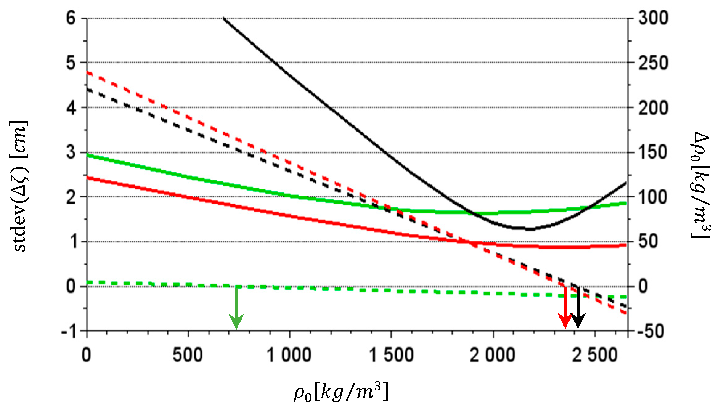
In the preliminary phase, the accuracy of the XGM2016 model, in terms of height anomalies, and the accuracy of the gravity prediction by the GGI method were estimated. These values are necessary for the correct estimation of the observation weights. To estimate the accuracy of gravity prediction, initial modeling was performed in a smaller, central part of the elaboration area for various ρ 0 values, assuming that the gravity errors adopted were at the level of ± 3   mGal ( 1   mGal = 10   μm / s 2 ). Based on this, the accuracy of the gravity prediction was estimated to be at the level of ± 2.2   mGal , which, as stated above, indicates that the gravity errors used to estimate the gravity weights should be approximately in the range ± ( 4 6 )   mGal . Therefore, the value of ± 5   mGal was adopted for further analyses. The height anomalies determined from the XGM2016 model were compared along the GSVS17 profile; with the mean height anomalies obtained from the 13 models participating in the Colorado geoid experiment hereinafter marked as ζ R e f [28]. The obtained standard deviation of the differences, at the level of ± 10   c m , was adopted for the weight estimation used in further calculations. So far, the GGI method has been applied to land plains and low mountains. For such areas, the significance of the adopted reference density model for the accuracy of the GGI model in terms of gravity values was demonstrated [41]. The currently analyzed area covers high mountains (average height over 2200 m and with the highest point above the height of 4000 m ) and the disturbing potential values used have lower weights, so their impact on the estimated densities will be smaller. Therefore, we can also expect a significant impact of the reference density model on the accuracy of the model, in terms of the height anomalies. To analyze this issue, a series of test calculations were performed, covering a wide range of reference densities ρ 0 (from 0 to 2670   k g / m 3 in increments between 100 and 500 k g / m 3 ) . We assumed that the size of the constant density zones was 6 × 6   k m . The calculations were performed for three versions of the gravity data used:
  • terrestrial-only,
  • airborne-only and
  • combined (with the use of terrestrial and airborne gravity data).
Height anomalies determined from the GGI model ( ζ G G I ) for each version of the gravity data and for different ρ 0 values were compared to the reference values ( ζ m ) for the GSVS17 points. The standard deviations of the differences, Δ ζ = ζ G G I ζ m , were next determined as the model accuracy parameters. Relations between these standard deviations and the ρ 0 values are presented in Figure 3 by solid lines. For each analyzed version of the reference density model, the mean density of the Ω volume ( ρ m e a n ) from the GGI model was also determined. This allowed us to state the value of the mean density changes Δ ρ 0 = ρ m e a n ρ 0 for each modeling cycle. These values are represented in Figure 3 by dotted lines. Individual versions of the gravity data used are marked with different colors: airborne-only = green, terrestrial-only = black, and combined = red.
The results presented in Figure 3 show a clear relationship between the reference constant density model and the accuracy of the height anomalies determined by the GGI method. The least accurate are the results for ρ 0 = 0   k g / m 3 . There is a noticeable increase in the accuracy with the increase in the reference density values up to an optimal range of ρ 0 , for which the accuracy is the highest. This optimal range is the narrowest for the terrestrial version and significantly wider for the two other versions
The optimal ranges of ρ 0 values for individual versions are presented in Table 1. The ranges were adopted as the ranges, giving an accuracy no worse than 0.2 c m from the best results.
The shown strong dependence of the GGI model accuracy on the ρ 0 values causes a certain problem for the estimation of the optimal density ( ρ 0 o p t i m a l ) giving the highest quasigeoid accuracy. The best solution of this problem would be the use of a set of accurate reference GNSS/levelling data for the estimation of the ρ 0 o p t i m a l value. In the absence of such data, it is necessary to rely on the experience in various implementations of the method. Taking into account the wide range of optimal ρ 0 values for the airborne-only and combined versions, it can be expected that for these versions, it will not be very difficult to estimate the ρ 0 o p t i m a l value based on experience. For the terrestrial-only version, however, it will be much more difficult. In this case, the range of optimal values of ρ 0 is relatively narrow. Moreover, beyond this range, the decrease in accuracy is significant (compared to the versions using airborne gravity data). Hence, some additional parameters supporting the determination of the ρ 0 o p t i m a l value should be indicated. In this regard, the Δ ρ 0 values defined above may turn out to be helpful. The relationships between Δ ρ 0 and ρ 0 values are represented in Figure 3 by dotted lines. Note that these relationships are linear for all versions. Importantly, for versions using terrestrial gravity data (terrestrial-only and combined), the values of Δ ρ 0 achieve 0 for a ρ 0 value inside or close to the optimal range. These values of reference density ( ρ 0 z e r o ), for individual versions, are marked in Figure 3 by arrows and can be used to estimate the ρ 0 o p t i m a l value. For the combined version, the ρ 0 z e r o value is in the middle of the optimal range, so we can assume ρ 0 o p t i m a l = ρ 0 z e r o . For the terrestrial-only version, there is a slight but visible shift of the ρ 0 z e r o value from ρ 0 o p t i m a l . This shift shows that the use of the ρ 0 z e r o value to estimate the ρ 0 o p t i m a l value requires a further, broader and more detailed analysis. However, the presented results give hope that in the terrestrial-only or combined versions, this will be an effective method.
The above analyses were performed by comparing the modeling results with the reference data on the GSVS17 profile points. The best results were obtained for the combined version; hence, the final quasigeoid model was determined for this data version. The ρ 0 o p t i m a l value, used in further calculations, for this version was computed based on the ρ 0 z e r o value, assuming the equality of both quantities. As the changes of Δ ρ 0 are linear, in order to determine the ρ 0 z e r o value, it is sufficient to find the value of Δ ρ 0 for two ρ 0 , e.g., for minimal ρ 0 m i n = 0   k g / m 3 and maximal ρ 0 m a x = 2700   k g / m 3   ( Δ ρ 0 m a x ) values, and then to determine the ρ 0 z e r o value by a simple relation:
ρ 0 z e r o = Δ ρ 0 m i n Δ ρ 0 m i n Δ ρ 0 m a x ( ρ 0 m a x ρ 0 m i n )

3.2. Determination of GGI Geoid and Quasi Geoid Models for Colorado Geoid Experiment Area

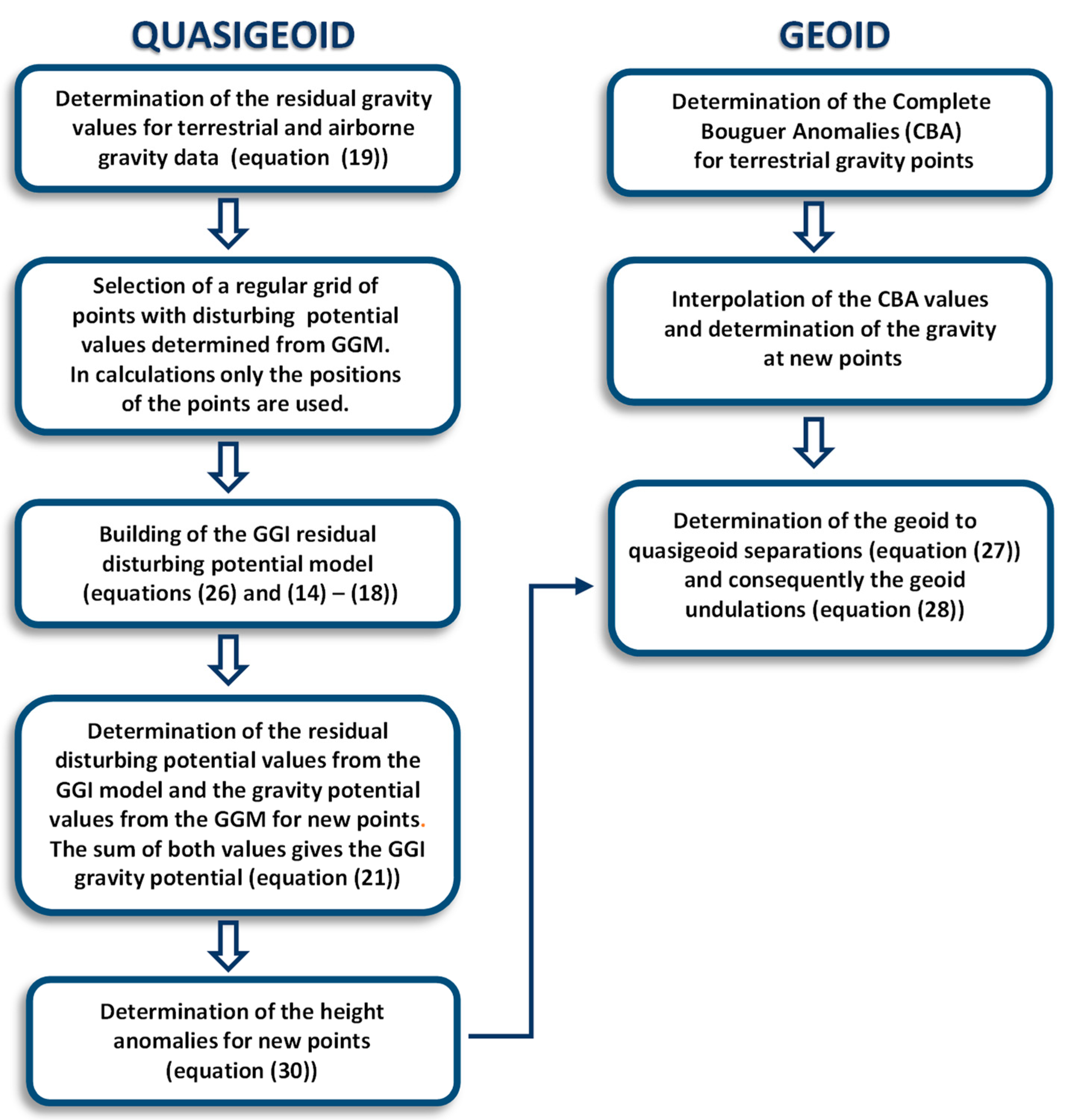
Geoid and quasigeoid models were determined according to the scheme presented in Figure 4.
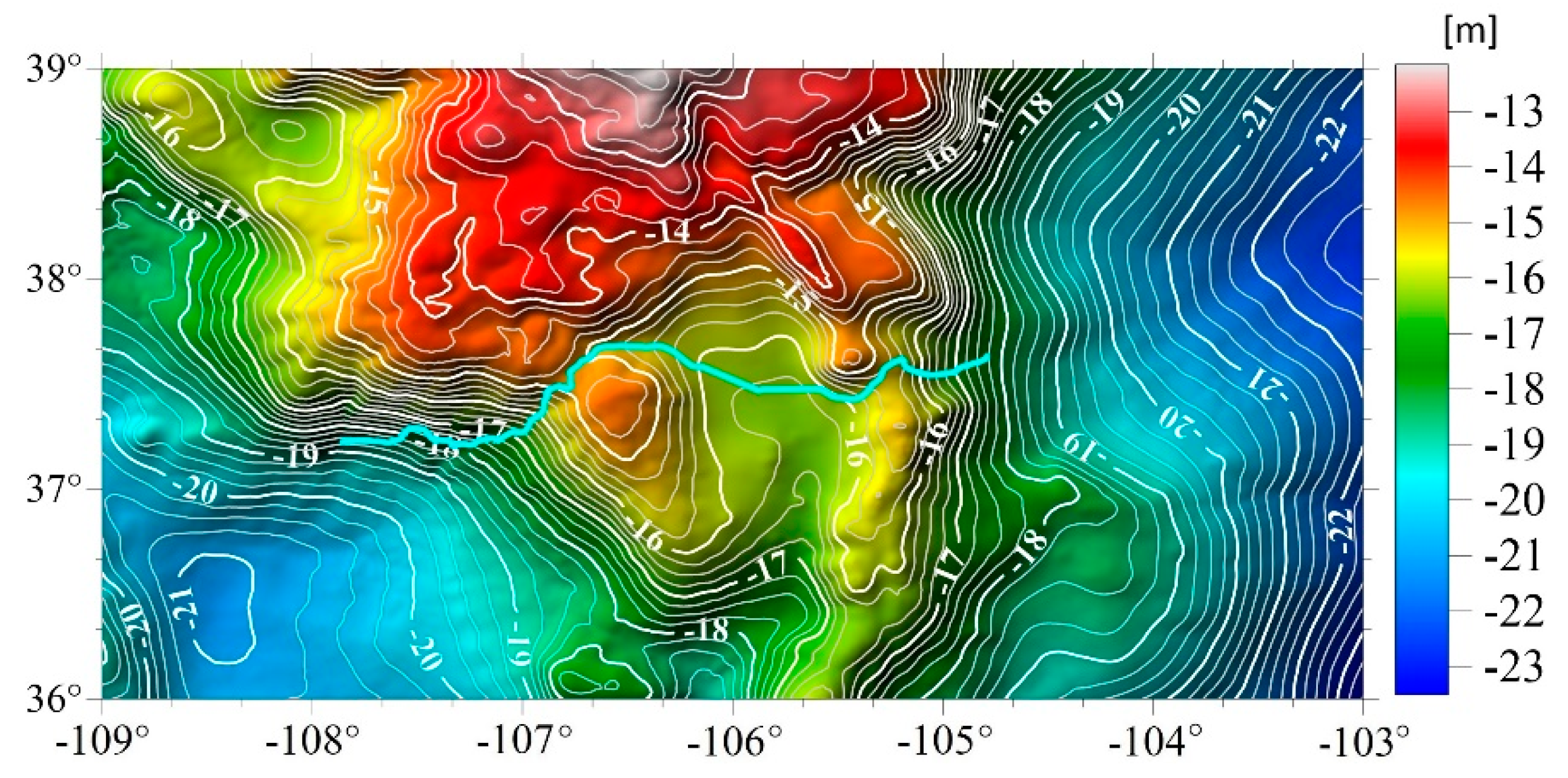
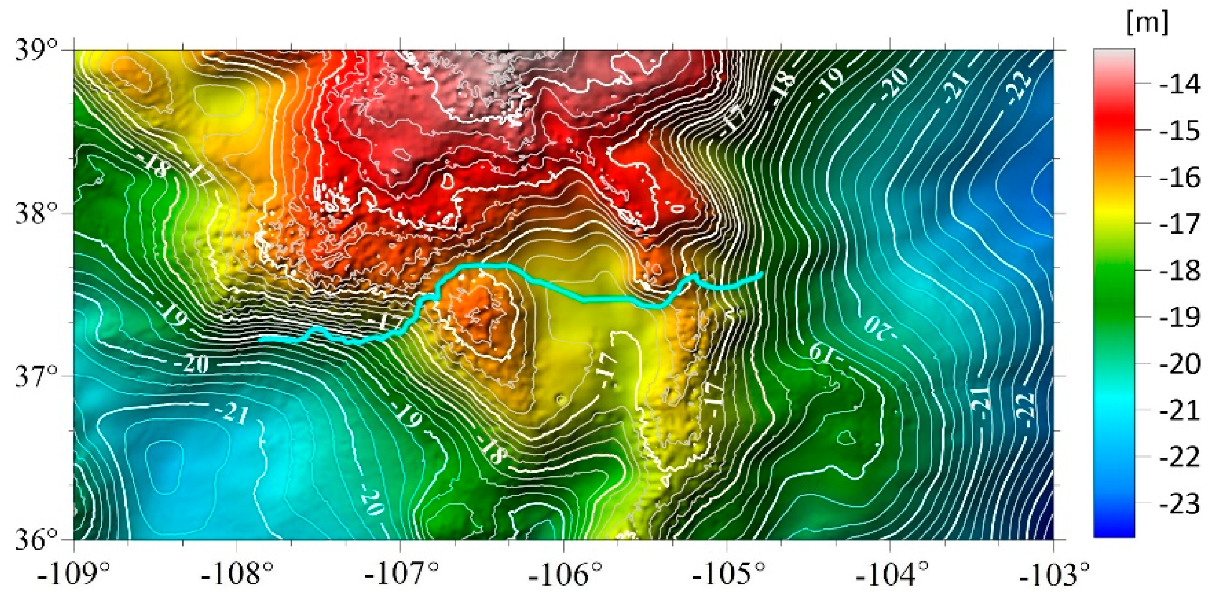
On the basis of the preliminary phase analyses, the gravity quasigeoid model was determined for the area used in the methods that participated in the Colorado geoid experiment. The data set presented in Figure 2 was used in the calculations. In this figure, the area for which the 1 × 1 grid of the quasigeoid model was determined is marked by the black line. In the calculations, zones of constant density with a size of 6 × 6   k m were assumed, and the ρ 0 o p t i m a l = ρ 0 z e r o value was determined using Equation (32). A map of the determined quasigeoid model is presented in Figure 5.
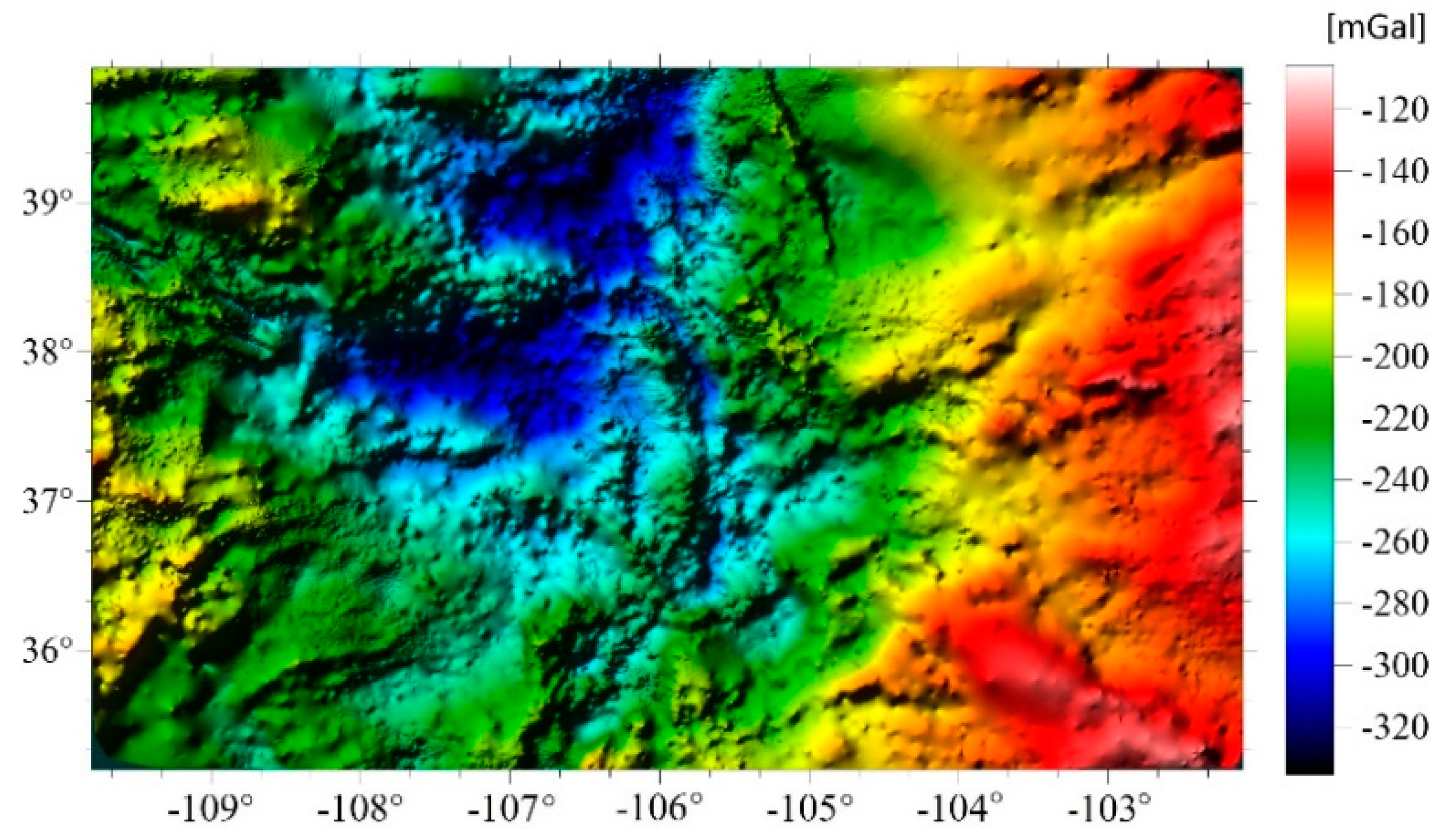
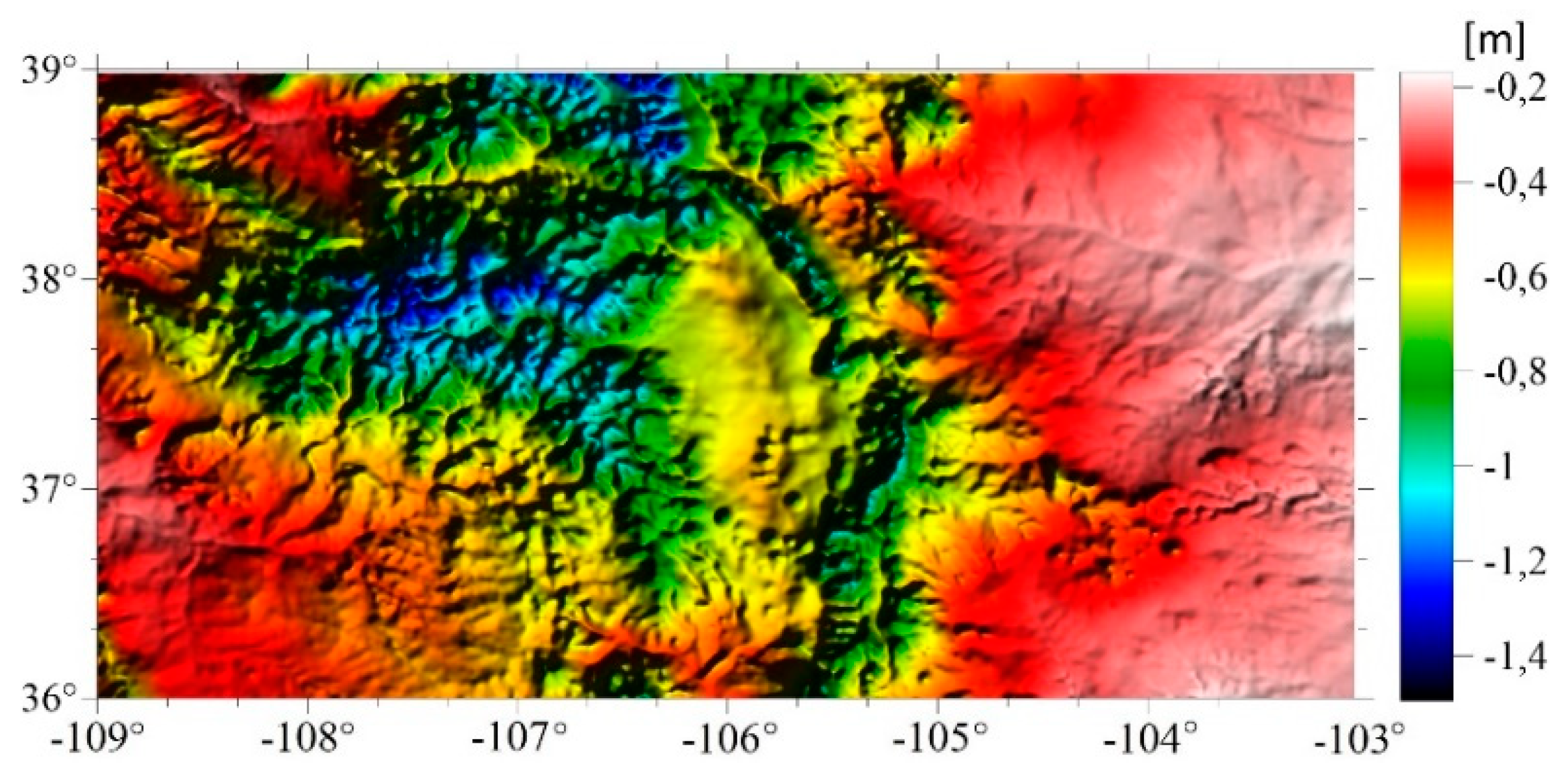
The geoid model was determined on the basis of the quasigeoid model, based on relation (28). The g ¯ values necessary to calculate the geoid to quasigeoid separation (27) were calculated according to formula (31). The gravity values g at each 1 × 1 grid point were determined by the interpolation of the complete Bouguer anomalies (CBA) using the kriging method. The CBA values were calculated using the same DEM as in the quasigeoid modeling, taking into account topographic masses within a radius of 167 k m and assuming their constant density ρ = 2670   k g / m 3 . Figure 6 shows the CBA values used for gravity prediction and Figure 7 presents the geoid to quasigeoid separations used for geoid model determination.
The map of the determined geoid model is presented in Figure 8.

4. Discussion

In order to evaluate the developed models, height anomalies ( ζ G G I ) and geoid undulations ( N G G I ) determined by the GGI method in the 1 × 1 grids were compared to the average values obtained from the models analyzed in the Colorado geoid experiment (13 for the quasigeoid and 14 for the geoid) at the GSVS17 points. These values for height anomalies are marked in the same way as before ( ζ m ), and for geoid undulations they are hereafter referred as N m . Subsequently, the differences Δ ζ = ζ G G I ζ m and Δ N = N G G I N m were determined, the basic statistics of which are presented in Table 2.
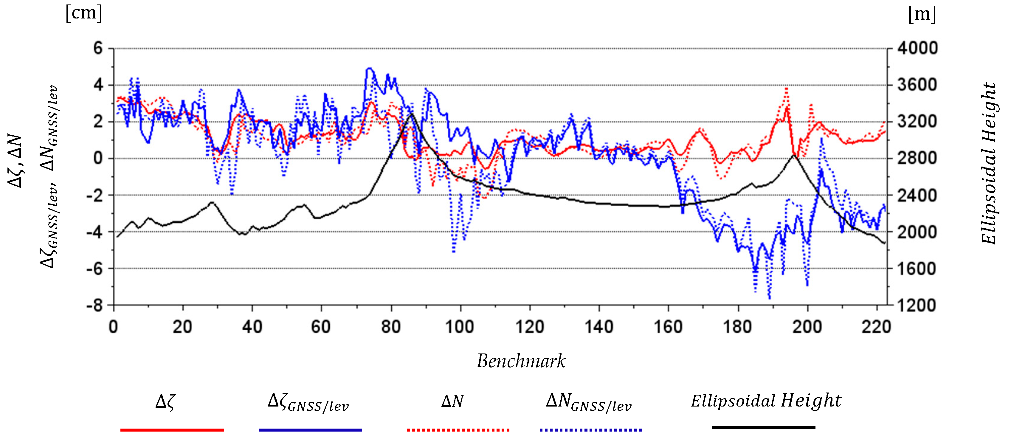
Ellipsoidal and Helmert orthometric heights measured at the GSVS17 profile points were used for the independent evaluation of the developed models. Based on the data provided, we determined the measured geoid undulations ( N G N S S / l e v ). The gravity values measured at the GSVS17 profile points were used to convert the Helmert orthometric heights into the normal heights (according to Equation (27)), and consequently we calculate the GNSS/levelling height anomalies ( ζ G N S S / l e v ) by the difference between the ellipsoidal and normal heights. Those values were compared to ζ G G I and N G G I values. Hence, the differences Δ ζ G N S S / l e v = ζ G G I ζ G N S S / l e v and Δ Δ G N S S / l e v = N G G I N G N S S / l e v were calculated; the basic statistics of which are also presented in Table 2.
All of the differences, the statistics of which are presented in Table 2, are also presented in Figure 9. From Δ ζ G N S S / l e v and Δ N G N S S / l e v , offsets of 90   c m (associated with the long-wavelength errors of the US vertical datum [51]) were removed.
The determined geoid and quasigeoid models were also compared with the N m and ζ m values for all 1 × 1 grids points. The most important statistics of the differences Δ ζ = ζ G G I ζ m and Δ N = N G G I N m are presented in Table 3.
When assessing the determined geoid and quasigeoid models, it is useful to refer to the results obtained by the methods participating in the Colorado geoid experiment. On the basis of [28], we summarized the ranges of the corresponding values obtained for all methods taking part in the experiment. These values are presented in Table 2; Table 3 in brackets, next to the values determined for the GGI method. Accepting the standard deviation (STD) values of the differences between the quantities determined by the GGI method and their reference values as the basic parameters of the accuracy assessment, we can determine the relation of the GGI method to the methods participating in the Colorado geoid experiment. The STD values determined in reference to the mean geoid and quasigeoid models, calculated based on the GSVS17 profile points (Table 2), were ± 0.9   c m  for the quasigeoid and ± 1.1   c m  for the geoid model. Using the results of [28], we can notice that only in one quasigeoid model and one geoid model from the Colorado geoid experiment were lower STD values obtained. The analogous STD values calculated on the basis of all 1 × 1  grid points (Table 3) are worse; they are ± 2.3   c m  and ± 2.6   c m  for the quasigeoid and geoid, respectively. Additionally, the relationships with the methods participating in the Colorado geoid experiment are worse. Slightly lower STD values were obtained for seven quasigeoid models and four geoid models. An independent evaluation of the developed models is their comparison with the GNSS/levelling height anomalies and geoid undulations. The STD values determined in reference to these values at the GSVS17 profile points (Table 2) for the quasigeoid and geoid models were ± 2.6   c m  and ± 2.5   c m , respectively. Among the Colorado geoid experiment models, lower STD values were obtained for three quasigeoid and three geoid models. It should also be noticed that there was a relatively small decrease or no decrease in the accuracy parameters of the determined geoid model in relation to the quasigeoid model. Taking into account the technique used for the determination of the geoid model, the accuracy of the obtained geoid–quasigeid separation should be assessed as high.
Note that the differences of both Δ ζ  and Δ N , represented in Figure 9 by red solid and dotted lines, respectively, are within very narrow ranges and are close to each other. The graphs of the differences Δ ζ G N S S / l e v  and Δ N G N S S / l e v  (blue solid and dotted lines) are also interesting. There is a clear change in their values in their final sections (approximately 80 endpoints of the profile). The shift of the mean values for the points in the start and end sections is at the level of 5   c m  and is also visible for other geoid and quasigeoid modeling methods participating in the Colorado geoid experiment [28]. This shift is the main reason for the significant increase in the STD values of the Δ ζ G N S S / l e v  and Δ N G N S S / l e v  differences.

5. Conclusions

The conducted analyses lead to several important GGI method conclusions. Primarily, the proposed use of the disturbing potential values determined from the GGM, instead of the GNSS/levelling data, turned out to be very effective. This allows for the determination of a local gravimetric quasigeoid model, fitted to the GGM used.
Test calculations were based on terrestrial and airborne gravity data. Such a data set made it possible to carry out analyses on the three versions of the gravity data used: terrestrial-only, airborne-only, and combined, which used the airborne and terrestrial datasets. The GGI models developed for each version turned out to be dependent on the reference density model adopted for the calculations. By comparing the determined quasigeoid models with the reference values obtained in the Colorado geoid experiment, it was possible to estimate the optimal density ranges giving the most accurate results. The narrowest and the most unfavorable range of optimal density values was obtained for the terrestrial-only version. Significantly wider ranges of the optimal values of ρ 0  (more favorable) were obtained for the version using airborne gravity data (airborne-only and combined). Moreover, the highest accuracy was achieved for the combined version (Table 1). Therefore, the supplementing of the data set with airborne gravity data leads to an improvement of the quality of geoid and quasigeoid models.
The demonstrated relationship between the accuracy of the GGI model and the ρ 0 value causes problems for determining an accurate quasigeoid model and indicates the need to determine or estimate the optimal ρ 0 as one of the most important parameters in the modeling process. At the present stage, the estimation of the optimal reference density model should be based on the GNSS/levelling control dataset. In the absence of such data, one could follow the results of previous applications of the method and the optimal ρ 0 estimation, the first of which are the presented results obtained by the Colorado geoid experiment. Analyses of changes in the mean density of topographic masses ( Δ ρ 0 = ρ m e a n ρ 0 ) can also be helpful in searching for the optimal ρ 0 values. For the terrestrial-only and combined versions, these values achieve 0 for a ρ 0 value inside or close to the optimal ranges. Therefore, they can be used for the estimation of the optimal densities for these versions. However, it should be clearly emphasized that the study of these relationships requires further analysis, mainly on the use of GGMs with different resolutions and for other types of terrain.
In the analyzed case, these relations allowed determining the optimal density for the combined version, for which the model in the form of a 1 × 1  grid was calculated in the same area used for the models determined in the Colorado geoid experiment. For the same grid, the geoid–quasigeoid separation was determined, and this was used to build the geoid model. The standard deviations of the differences between the geoid and quasigeoid models determined by the GGI method and the mean models determined for the GSVS17 profile points were ± 0.9   c m for the quasigeoid and ± 1.2   c m for the geoid model. Analogous values, determined on the basis of all 1 × 1 grid points, were ± 2.3   c m and ± 2.6   c m for the quasigeoid and geoid models, respectively. The presented results indicate the high-quality of the determined quasigeoid and geoid models. A relatively small difference between the accuracy parameters of the geoid and the quasigeoid also proves that this was a very accurate determination of the geoid-quasigeoid separation.

Author Contributions

Conceptualization, M.T.; methodology, M.T.; software, M.T.; validation, Y.M.W. and M.O.-W.; formal analysis, O.J.; investigation, M.O.-W.; resources, Y.M.W.; data curation, Y.M.W.; writing—original draft preparation, M.T., O.J. and M.O.-W.; writing—review and editing, M.T. and Y.M.W.; visualization, O.J.; supervision, M.T. All authors have read and agreed to the published version of the manuscript.

Funding

This research received no external funding.

Institutional Review Board Statement

Not applicable.

Informed Consent Statement

Not applicable.

Conflicts of Interest

The authors declare no conflict of interest.

References

  1. Heiskanen, W.A.; Moritz, H. Physical Geodesy; W. H. Freeman and Company: New York, NY, USA, 1967. [Google Scholar]
  2. Hofmann-Wellenhof, B.; Moritz, H. Physical Geodesy; Springer: Berlin/Heidelberg, Germany, 2005. [Google Scholar]
  3. Torge, W. Geodesy, 3rd ed.; Walter de Gruyter: Berlin/Heidelberg, Germany; New York, NY, USA, 2001. [Google Scholar]
  4. Vanicek, P.; Kleusberg, A. The Canadian geoid-stokesian approach. Manuscr. Geod. 1987, 12, 86–98. [Google Scholar]
  5. Sjöberg, L.E. On the topographic effects by the Stokes-Helmert method of geoid and quasigeoid determination. J. Geod. 2000, 74, 255–268. [Google Scholar]
  6. Heck, B. On Helmert’s methods of condensation. J. Geod. 2003, 77, 155–170. [Google Scholar] [CrossRef]
  7. Huang, J.; Véronneau, M. Canadian gravimetric geoid model 2010. J. Geod. 2013, 87, 771–790. [Google Scholar] [CrossRef]
  8. Forsberg, R. A Study of Terrain Reductions, Density Anomalies and Geophysical Inversion Methods in Gravity Field Modelling; Report 355; Department of Geodetic Science, The Ohio State University: Columbus, OH, USA, 1984. [Google Scholar]
  9. Forsberg, R. Terrain effects in geoid computation. In Lecture Notes, International School for the Determination and Use of the Geoid; International Geoid Service, DIIAR—Politecnico di Milano: Milano, Italy, 1994; pp. 101–134. [Google Scholar]
  10. Forsberg, R.; Tscherning, C.C. Topographic effects in gravity field modelling for BVP. In Geodetic Boundary Value Problems in View of the One Centimeter Geoid; Lecture Notes in Earth Sciences, 65, Sansó, F., Rummel, R., Eds.; Springer: Berlin/Heidelberg, Germany, 1997; pp. 121–160. [Google Scholar]
  11. Omang, O.C.D.; Forsberg, R. How to handle the topography in geoid determination: Three examples. J. Geod. 2003, 74, 458–466. [Google Scholar] [CrossRef]
  12. Abd-Elmotaal, H.; Kühtreiber, N. Geoid Determination Using Adapted Reference Field, Seismic Moho Depths and Variable Density Contrast. J. Geod. 2003, 77, 77–85. [Google Scholar] [CrossRef]
  13. Forsberg, R. Gravity field terrain effect computations by FFT. Bull. Géod. 1985, 59, 342–360. [Google Scholar] [CrossRef]
  14. Schwarz, K.P.; Sideris, M.G.; Forsberg, R. Use of FFT methods in physical geodesy. Geophys. J. Int. 1990, 100, 485–514. [Google Scholar] [CrossRef] [Green Version]
  15. Forsberg, R.; Sideris, M.G. Geoid computation by the multi-band spherical FFT approach. Manuscr. Geod. 1993, 18, 82–90. [Google Scholar]
  16. Sideris, M.G. Geoid determination by FFT techniques. In Lecture Notes, International School for the Determination and Use of the Geoid; International Geoid Service, DIIAR—Politecnico di Milano: Milano, Italy, 1994. [Google Scholar]
  17. Haagmans, R.; de Min, E.; Van Gelderen, M. Fast evaluation of convolution integrals on the sphere using 1D FFT and a comparison with existing methods for Stokes’ integral. Manuscr. Geod. 1993, 18, 227–241. [Google Scholar]
  18. Sjöberg, L.E. Refined least squares modification of Stokes’ formula. Manuscr. Geod. 1991, 16, 367–375. [Google Scholar]
  19. Sjöberg, L.E. A general model for modifying Stokes’ formula and its least squares solution. J. Geod. 2003, 77, 459–464. [Google Scholar] [CrossRef]
  20. Sjöberg, L.E. A computational scheme to model the geoid by the modified Stokes formula without gravity reductions. J. Geod. 2003, 77, 423–432. [Google Scholar] [CrossRef]
  21. Sjöberg, L.E. A local least-squares modification of Stokes’ formula. Stud. Geoph. Geod. 2005, 49, 23–30. [Google Scholar] [CrossRef]
  22. Freeden, W.; Gervens, T.; Schreiner, M. Constructive Approximation on the Sphere with Applications to Geomathematics; Oxford University Press on Demand: Oxford, UK, 1998. [Google Scholar]
  23. Freeden, W.; Michel, V. Multiscale Potential Theory: With Applications to Geoscience; Birkhäuser: Basel, Switzerland, 2004. [Google Scholar]
  24. Schmidt, M.; Han, S.C.; Kusche, J.; Sanchez, L.; Shum, C. Regional high-resolution spatiotemporal gravity modeling from GRACE data using spherical wavelets. Geophys. Res. Lett. 2006, 33, L08403. [Google Scholar] [CrossRef] [Green Version]
  25. Schmidt, M.; Fengler, M.; Mayer-Gürr, T.; Eicker, A.; Kusche, J.; Sánchez, L.; Han, S.C. Regional gravity modeling in terms of spherical base functions. J. Geod. 2007, 81, 17–38. [Google Scholar] [CrossRef] [Green Version]
  26. Klees, R.; Tenzer, R.; Prutkin, I.; Wittwer, T. A data-driven approach to local gravity field modelling using spherical radial basis functions. J. Geod. 2008, 82, 457–471. [Google Scholar] [CrossRef] [Green Version]
  27. Liu, Q.; Schmidt, M.; Sánchez, L.; Willberg, M. Regional gravity field refinement for (quasi-) geoid determination based on spherical radial basis functions in Colorado. J. Geod. 2020, 94, 99. [Google Scholar] [CrossRef]
  28. Wang, Y.M.; Sánchez, L.; Agren, J.; Huang, J.; Forsberg, R.; Abd-Elmotaal, H.; Barzaghi, R.; Bašić, T.; Carrion, D.; Claessens, S.; et al. Colorado geoid computation experiment—Overview and summary. J. Geod. Special Issue on Reference Systems in Physical Geodesy (under review). 2021. [Google Scholar]
  29. Ligas, M.; Kulczycki, M. Kriging and moving window kriging on a sphere in geometric (GNSS/levelling) geoid modelling. Surv. Rev. 2018, 50, 155–162. [Google Scholar] [CrossRef]
  30. Zhong, D. Robust estimation and optimal selection of polynomial parameters for the interpolation of GPS geoid heights. J. Geod. 1997, 71, 552–561. [Google Scholar] [CrossRef]
  31. Das, R.K.; Samanta, S.; Jana, S.K.; Rosa, R. Polynomial interpolation methods in development of local geoid model. Egypt. J. Remote Sens. Space Sci. 2017, 21, 265–271. [Google Scholar] [CrossRef]
  32. Lin, L. Application of a back-propagation artificial neural network to regional grid-based geoid model generation using GPS and leveling data. J. Surv. Eng. 2007, 133, 81–89. [Google Scholar] [CrossRef] [Green Version]
  33. Cakir, L.; Yilmaz, N. Polynomials, radial basis functions and multilayer perceptron neural network methods in local geoid determination with GPS/levelling. Measurement 2014, 57, 148–153. [Google Scholar] [CrossRef]
  34. Trojanowicz, M. Local modelling of quasigeoid heights with the use of the gravity inverse method—Case study for the area of Poland. Acta Geodyn. Geomater. 2012, 9, 5–18. [Google Scholar]
  35. Trojanowicz, M.; Osada, E.; Karsznia, K. Precise local quasigeoid modelling using GNSS/levelling height anomalies and gravity data. Surv. Rev. 2020, 52, 76–83. [Google Scholar] [CrossRef]
  36. Banasik, P.; Bujakowski, K.; Kudrys, J.; Ligas, M. Development of a precise local quasigeoid model for the city of Krakow—QuasigeoidKR2019. Rep. Geod. Geoinform. 2020, 109, 25–31. [Google Scholar] [CrossRef]
  37. Trojanowicz, M. Assessment of the accuracy of local quasigeoid modelling using the GGI method: Case study for the area of Poland. Studia Geophys. Geod. 2015, 59, 505–523. [Google Scholar] [CrossRef]
  38. Łyszkowicz, A. Quasigeoid for the area of Poland computed by least squares collocation. Tech. Sci. 2010, 13, 147–163. [Google Scholar] [CrossRef]
  39. Szelachowska, M.; Kryński, J. GDQM-PL13—the new gravimetric quasigeoid model for Poland. Geoinf. Issues 2014, 6, 5–19. [Google Scholar]
  40. Trojanowicz, M. Local disturbing potential model with the use of geophysical gravity data inversion—case study in the area of Poland. Acta Geodyn. Geomater. 2019, 16, 293–299. [Google Scholar] [CrossRef]
  41. Trojanowicz, M.; Owczarek-Wesołowska, M.; Pospíšil, L.; Jamroz, O. Determination of the Selected Gravity Field Functionals by the GGI Method: A Case Study of the Western Carpathians Area. Appl. Sci. 2020, 10, 7892. [Google Scholar] [CrossRef]
  42. Trojanowicz, M.; Owczarek-Wesołowska, M.; Wang, Y.M.; Jamroz, O. Gravimetric quasigeoid modelling by the GGI method in the Colorado mountains area. In Proceedings of the Scientific Assembly of the International Association of Geodesy, Beijing, China, 28 June–2 July 2021. [Google Scholar]
  43. Trojanowicz, M. Local quasigeoid modelling using gravity data inversion technique—Analysis of fixed coefficients of density model weighting matrix. Acta Geodyn. Geomater. 2012, 9, 269–281. [Google Scholar]
  44. Blakely, R.J. Potential Theory in Gravity and Magnetic Applications; Cambridge University Press: Cambridge, UK, 1995. [Google Scholar]
  45. Nagy, D. The gravitational attraction of right angular prism. Geophysics 1966, 31, 362–371. [Google Scholar] [CrossRef]
  46. Nagy, D.; Papp, G.; Benedek, J. The gravitational potential and its derivatives for the prism. J. Geod. 2001, 74, 552–560. [Google Scholar] [CrossRef]
  47. Li, Y.; Oldenburg, D.W. 3-D inversion of gravity data. Geophysics 1998, 63, 109–119. [Google Scholar] [CrossRef]
  48. Sánchez, L.; Agren, J.; Huang, J.; Wang, Y.; Forsberg, R. Basic Agreements for the Computation of Station Potential Values as IHRS Coordinates, Geoid Undulations and Height Anomalies within the Colorado 1 cm Geoid Experiment. Available online: https://ihrs.dgfi.tum.de/fileadmin/JWG_2015/Colorado_Experiment_Basic_req_V0.5_Oct30_2018.pdf (accessed on 21 October 2021).
  49. Mäkinen, J.; Ihde, J. The Permanent Tide in Height Systems. In Observing Our Changing Earth; Internation Association of Geodesy Symposia 133; Sideris, M.G., Ed.; Springer: Berlin/Heidelberg, Germany, 2009. [Google Scholar]
  50. Pail, R.; Fecher, T.; Barnes, D.; Factor, J.; Holmes, S.; Gruber, T.; Zingerle, P. The experimental gravity field model XGM2016. GFZ Data Serv. 2017. [Google Scholar] [CrossRef]
  51. Wang, Y.M.; Saleh, J.; Li, X.; Roman, D.R. The US Gravimetric Geoid of 2009 (USGG2009): Model development and evaluation. J. Geod. 2012, 86, 165–180. [Google Scholar] [CrossRef]
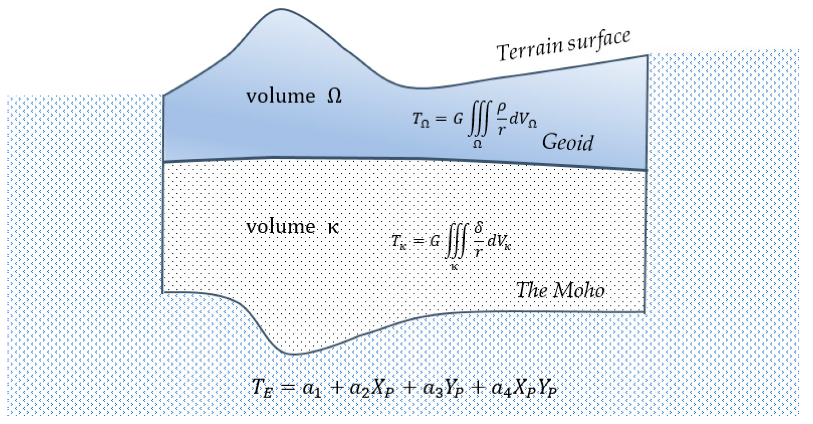
Figure 1. Components defining the disturbing potential model used in the GGI method.
Remotesensing 13 04217 g001
Figure 2. Data accepted for the calculations. (a) airborne gravity points: light blue dots; terrestrial gravity points: dark blue dots. (b) The DEM, which defines the horizontal range of the Ω and κ volumes; white dots: positions of points with known disturbing potential values from GM. Red lines show the location of the GSVS17 profile points and black lines define the area for which the geoid and quasigeoid models with a 1 × 1 grid were determined.
Remotesensing 13 04217 g002
Figure 3. Standard deviations of differences Δ ζ = ζ G G I ζ m (solid lines) and Δ ρ 0 = ρ m e a n ρ 0 values (dotted lines) as functions of reference densities ρ 0 for the following versions: airborne-only (green), terrestrial-only (black), and combined (red). ρ 0 z e r o values for each version are marked by arrows.
Remotesensing 13 04217 g003
Figure 4. Stages of the geoid and quasigeoid model determination.
Remotesensing 13 04217 g004
Figure 5. Map of the quasigeoid model determined using the GGI method. The light blue line is the location of the GSVS17 profile.
Remotesensing 13 04217 g005
Figure 6. Map of CBA values used for gravity prediction.
Remotesensing 13 04217 g006
Figure 7. Map of geoid to quasigeoid separations used to determine the geoid model.
Remotesensing 13 04217 g007
Figure 8. Map of geoid model determined by GGI method. The light blue line is the location of the GSVS17 profile.
Remotesensing 13 04217 g008
Figure 9. The differences Δ ζ = ζ G G I ζ m , Δ N = N G G I N m , Δ ζ G N S S / l e v = ζ G G I ζ G N S S / l e v , Δ N G N S S / l e v = N G G I N G N S S / l e v , and ellipsoidal heights at GSVS17 points. From the Δ ζ G N S S / l e v and Δ N G N S S / l e v , offsets of 90   c m were removed.
Remotesensing 13 04217 g009
Table 1. Optimal ranges of ρ 0 values and estimated quasigeoid accuracy based on ζ m values in the GSVS17 profile points.
VersionThe Optimal Range of ρ 0 Minimal Accuracy in the Optimal RangeThe Best Accuracy in the Optimal Range
Unit k g / m 3 cmcm
Terrestrial only2000–23001.51.3
Airborne only1200–26701.91.7
Combined1700–26701.10.9
Table 2. Basic statistics of the differences Δ ζ = ζ G G I ζ m , Δ N = N G G I N m , as well as Δ ζ G N S S / l e v = ζ G G I ζ G N S S / l e v and Δ N G N S S / l e v = N G G I N G N S S / l e v , based on the GSVS17 profile points (in centimeters). In brackets are ranges of corresponding values obtained for methods participating in the Colorado geoid experiment (based on [28]).
MinMaxMeanRMSStdevRange
Δ ζ −0.53.31.11.4 (1.0 ÷   3.4)0.9 (0.7 ÷   2.4)3.9 (3.4 ÷   13.9)
Δ N −2.33.91.01.5 (1.3 ÷   3.6)1.2 (1.1 ÷   2.9)6.2 (6.8 ÷   16.6)
Δ ζ G N S S / l e v 83.894.990.290.22.6 (1.8 ÷   3.6)11.2 (10.7 ÷   17.1)
Δ N G N S S / l e v 82.394.789.489.92.5 (2.0 ÷   4.1)12.4 (10.0 ÷   25.1)
Table 3. Basic statistics of the differences Δ ζ = ζ G G I ζ m and Δ N = N G G I N m based on all 1 × 1 grids points (in centimeters). In brackets are the ranges of corresponding values obtained for methods participating in the Colorado geoid experiment (based on [28]).
MinMaxMeanRMSStdevRange
Δ ζ −10.514.21.42.7 (1.6 ÷   5.2)2.3 (1.5 ÷   5.2)24.6 (18.0 ÷   70.0)
Δ N −17.517.01.43.0 (2.3 ÷   5.6)2.6 (2.1 ÷   5.6)34.4 (25.5 ÷   68.7)
Publisher’s Note: MDPI stays neutral with regard to jurisdictional claims in published maps and institutional affiliations.