Article

Mapping Global Urban Impervious Surface and Green Space Fractions Using Google Earth Engine

1
Key Laboratory of Land Surface Pattern and Simulation, Institute of Geographic Sciences and Natural Resources Research, Chinese Academy of Sciences, Beijing 100101, China
2
College of Resource and Environment, University of Chinese Academy of Sciences, Beijing 100049, China
3
School of Geographical Sciences, Fujian Normal University, Fuzhou 350007, China
*
Author to whom correspondence should be addressed.
Remote Sens. 2021, 13(20), 4187; https://doi.org/10.3390/rs13204187
Submission received: 18 September 2021 / Revised: 15 October 2021 / Accepted: 15 October 2021 / Published: 19 October 2021

Abstract

:
Urban impervious surfaces area (ISA) and green space (GS), two primary components of urban environment, are pivotal in detecting urban environmental quality and addressing global environmental change issues. However, the current global mapping of ISA and GS is not effective enough to accurately delineate in urban areas due to the mosaicked and complex structure. To address the issue, the hierarchical architecture principle and subpixel metric method were applied to map 30 m global urban ISA and GS fractions for the years 2015 and circa 2020. We use random forest algorithms for retrieval of the Normalized Settlement Density Index and Normalized Green Space Index from Landsat images using Google Earth Engine. The correlation coefficients of global urban ISA and GS fractions were all higher than 0.9 for 2015 and circa 2020. Our results show global urban ISA and GS areas in circa 2020 were 31.19 × 10⁴ km2 and 17.16 × 10⁴ km2, respectively. The novel ISA and GS fractions product can show potential applications in assessing the effects of urbanization on climate, ecology, and urban sustainability.

Graphical Abstract

1. Introduction

Global urbanization promotes social–economic development, which profoundly affects ecosystem services and environmental sustainability. Humans are the dominant drivers of the land-use/cover change from rural to urban as they seek to improve their well-being [1,2]. Currently, urban areas accommodate 55% of the global population, contribute 75% of global gross domestic product (GDP), and produce 75% of global carbon emissions in energy use [3,4]. Cities symbolize the most intensified land-use activities within coupled human–environment systems [5]. As a result, urbanization can influence the biophysical and biochemical processes, i.e., land-cover change, surface radiation and energy changes, hydrologic processes, and materials cycles, among others [6,7,8,9], all of which affect cropland encroachments, urban heat islands, rain flood disasters, biodiversity loss, and climate change in many ways [10,11,12]. Therefore, new knowledge about global urban land cover is essential to address urban-related issues of environmental sustainability through science–policy interfaces [4,13].
As the two foundation components of urban land or built-up areas, urban impervious surface area (ISA) and green space (GS) are important for building a better urban future that is livable, comfortable, and sustainable (https://unhabitat.org/ (accessed on 12 April 2021)). A series of indexes on sustainable cities and communities in the sustainable development goals (SDGs) for 2030 (https://sdgs.un.org/ (accessed on 12 April 2021)) were proposed for urban land cover, such as the ratio of land consumption rate to population growth rate and the average share of a built-up area that is open space for public use. Thus, fine-scale and timely urban land-cover maps are required for urban planning, spatial governance, and sustainability assessment to attain the SDGs. State-of-the-art technologies of urban land-cover mapping have advanced toward higher spatiotemporal resolution and accuracy [14,15,16]. In their initial stage, Moderate Resolution Imaging Spectroradiometer (MODIS) and Defense Meteorological Satellite Program/Operational Linescan System (DMSP/OLS) images from 250 m to 1 km resolution were utilized to map the global urban extent and ISA [13,17,18,19,20,21]. Recently, Landsat, Sentinel, and higher-resolution images were adopted to retrieve the urban extent or ISA with less than 30 m resolution [9,22,23,24,25,26,27,28,29], while the magnitude, rate and spatial heterogeneity of global urban change and their impacts on land-system and environment sustainability were assessed based on spatially explicit information [26].
In contrast, the development of urban GS datasets does not have sufficient resolution and completeness, due to varied definitions of green space and different monitoring methods [30]. The pan-European CORINE Land Cover data set contains a designated class “Green Urban Areas,” including GS larger than 25 ha [31].The Urban Atlas [32] for the EU and the Trust for Public Land’s ParkServe data set [33] for the US contains land-use information only for selected cities. Therefore, it is necessary to integrate multisource data fusion to create a comprehensive urban GS dataset to realize the monitoring and evaluation of urban GS across multiple cities. In a comparative study of urban GS in Poland using five open-source data, the results reveal large differences in the total amount of urban GS in the cities as depicted in different datasets [34]. Recently, developments in very high resolution (VHR) satellite remote sensing systems have begun to provide reliable and reproducible information on urban vegetation across large areas [30,35]. However, because urban GS monitoring is carried out in only a few cities or regions, high-precision mapping of global urban GS is still a significant challenge.
Global urban land mapping has made massive progress toward finer-scale and higher-spatiotemporal resolutions, which is attributed to the applications of big data and the cloud platform; for example, Google Earth Engine (GEE) remarkably enhances the data-processing capacity [9,14]. However, the spatially explicit metrics for global cities are defective in the systemic recognition of urban underlying environments and knowledge acquisition for the important science-to-practice continuum [36,37]. Those concepts, such as built-up area, urban land, constructed ISA, human settlement, and artificial ISA are often confusing and inconsistent with corresponding spatial extents, in which their spatial domains are actually different. Therefore, urban and rural settlements are not effectively differentiated, and the area of urban land is overestimated [9,17,18,19,20,22,23,24,25,26,27,28]. A number of researchers regard artificial ISA as built-up area or urban land, which may be misleading when scientists relay potential implications to practitioners [25,26]. We conducted a comparison and an analysis of the thirteen mainstream datasets that show large discrepancies between the different data products (Table S1).
The built-up environment of cities is usually complex in composition and structure with varied function areas and land uses/covers, with mosaics of buildings, roads, squares, some trees, and lawns [38,39]. Therefore, a large number of mixed-pixel ISA, GS, and other cover types occur despite Landsat images with 30-m resolution [40] or Sentinel images at 10-m resolution. The majority of global urban land-cover mapping relies on “hard classifications” in specific ISA and GS types. These classification results restrict the comprehensive evaluation of urban hydrological process, heat island intensity, and vegetation layout in urban planning.
To address those issues, a number of studies have combined the principle of spatial autocorrelation or used spatial structure information as a priori models to conduct subpixel mapping analyses of low- and medium-resolution images [41,42,43,44,45,46,47]. In our research, we used linear spectral mixture analysis and regression tree (RT) algorithms to decompose the mixed pixels of urban ISA and GS at national and urban scales—i.e., the ISA mapping from the National Land Cover Dataset (NLCD) in the USA and GS fraction mapping from China’s Land Use/cover Dataset (CLUD)—and at city scale in Beijing, Shanghai, Guangzhou, Chicago, New York, and Los Angeles [38,40,48]. Big data, cloud computing, and application of human digital interpretation [38] were also utilized to timely and accurately delineate urban built-up environment [13,14]. We used the random forest (RF) method to map the global urban ISA and GS fractions by subpixel classification. Then, we generated a series of datasets from urban boundaries to ISA and GS fractions.

2. Materials and Methods

2.1. The Principle and Strategies for Developing Urban ISA and GS Products

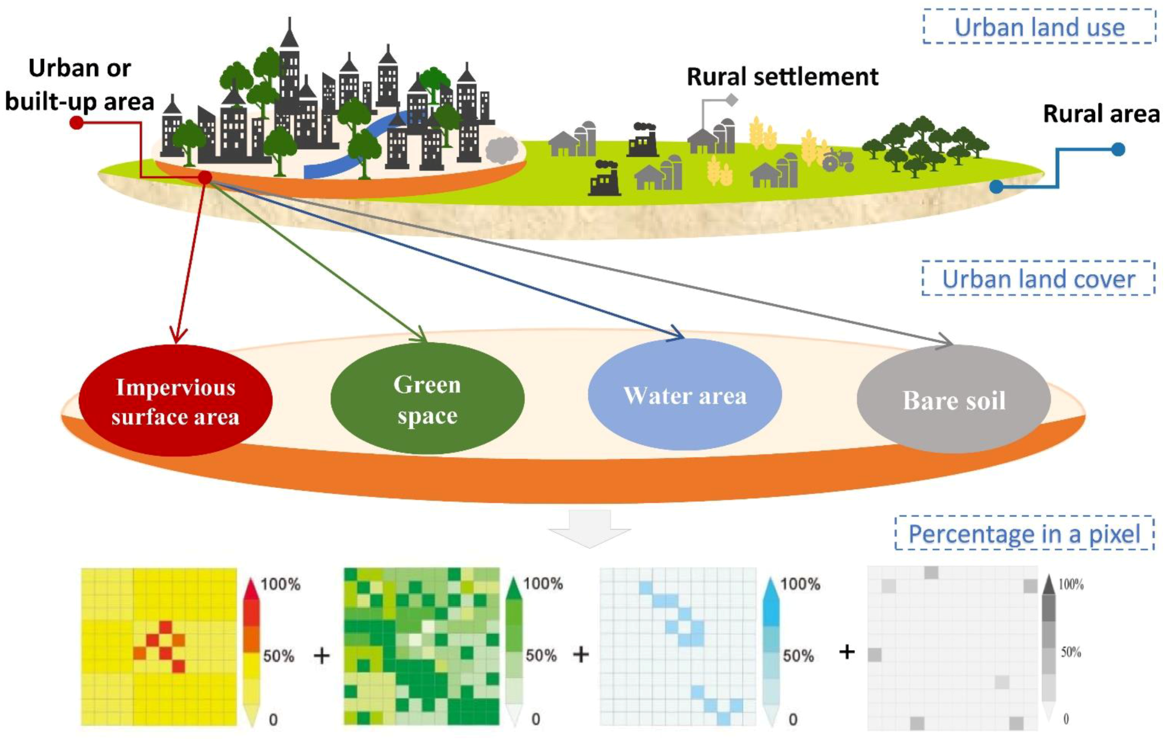
2.1.1. The Hierarchical Architecture Principle and Subpixel Metric Method

Urban areas closely related to human activities have the characteristics of complex landscape structure and spatial heterogeneity. In order to accurately describe the internal characteristics of a city, we further classified the urban and rural construction land, the independent industrial zone on the edge of the city, and the traffic zone through visual interpretation [40,49]. From the perspective of land use, the built-up areas are identified as a homogeneous unit through the segmentation of urban–rural boundaries according to their spatial configuration and intensity [49]. Therefore, human settlements adhere to a hierarchical architecture principle in spatial domains in line with construction activities. Among them, built-up areas manifest spatially explicit mosaics of dominant buildings, roads, squares, trees, lawns, or other cover types [39]. Here, the urban or built-up areas were usually decomposed into ISA, GS, water area (WA), and bare soil (BS) fractions at pixel scale as the percentage of land-cover composites (Figure 1).
According to the principle, ISA and GS located in built-up areas were mapped with percentages of pixels. These fractions can be expressed as
U r b a n = I S A G S W A B S
I S A P + G S P + W A P + B S P = 100 %
where Urban represents the urban or built-up area, which is composed of ISA, GS, WA, and BS. ISAp, GSp, WAp, and BSp represent the percentage of different fractions in pixels. The ISA and GS fractions were mapped on the GEE platform from Landsat images and the visualization of maps, such as images acquired by Google Earth, Gaofen-2 (GF-2), etc. [13,38].

2.1.2. The Mapping Strategies for ISA and GS Products

According to the above principle, the strategies for mapping the urban ISA and GS were developed based on Landsat images in 2015 and circa 2020 using the GEE platform. Five major steps were conducted: data collection and preprocessing, retrieval of the Normalized Settlement Density Index (NSDI) and Normalized Green Space Index (NGSI), identification of urban–rural boundaries, mapping urban ISA and GS, and quality control and accuracy validation of the ISA and GS (Figure 2).

2.1.3. Data Collection and Preprocessing

The preprocessing of the data was carried out on GEE, including cloud masking, band combination, image mosaic creation, image fusion, and other preprocesses. The data sources were mainly Landsat OLI with a spatial resolution of 30 m. VIIRS day/night, and SRTM digital elevation model (DEM) data were also used as input parameters in the calculations to map urban ISA and GS products. Google Earth and GF-2 images were used for the accuracy assessments (Table 1).

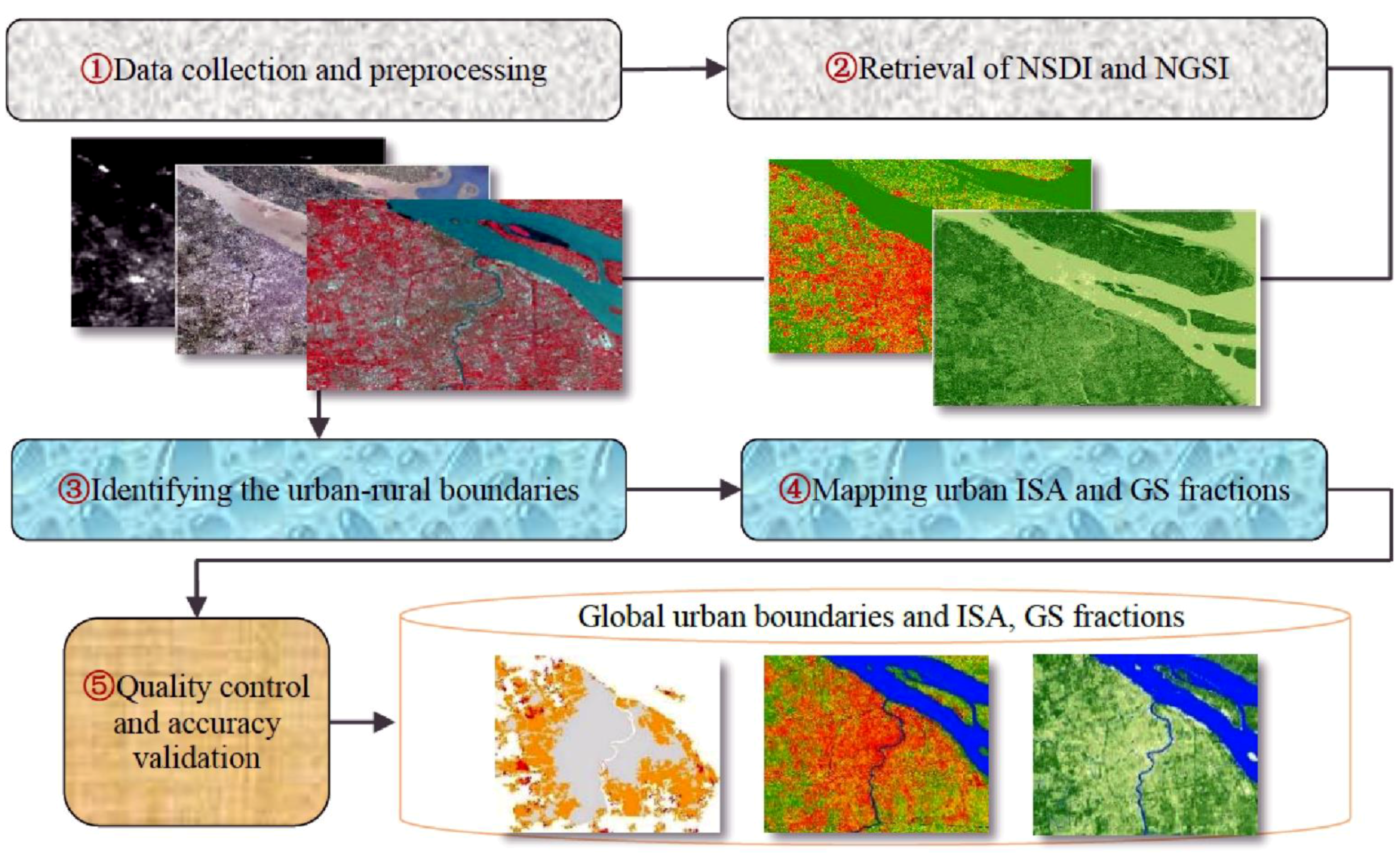
2.2. Mapping Global Urban ISA and GS Using GEE

2.2.1. Retrieval of NSDI and NGSI

The algorithms and codes for mapping urban ISA and GS were developed on the GEE platform. The annual maximum NDVI values in 2015 and circa 2020 were derived from Landsat 8 OLI. According to the principle of NDVI invariant region extraction, the NDVI in circa 2020 and 2015 was subtracted to extract the areas where the NDVI was basically unchanged. We randomly select 300 points in the urban area and generate a 90 m × 90 m grid on each point. Based on these grids, the GF-2 image was visually interpreted, and the sample grid digitized into ISA and GS (Figure 3). After that, the impervious fraction attributes corresponding to each grid were calculated to generate training samples, which were used in the subsequent RF algorithm.
Due to the large differences in climate, land use, vegetation covers, and social–economic conditions among the urban ecoregions, Schneider et al. separated global terrestrial land into sixteen urban ecoregions [18]. There is no urban distribution in the permanent ice region, so we choose 57 sample cities from the other fifteen ecoregions to train our samples (Figure 4). The NSDI was used to calculate the proportion of ISA in the grid. Each urban ecoregion’s NSDI (the ISA percentage within each pixel) was generated based on an RF algorithm on the GEE platform.
The RF algorithm is a supervised learning regression algorithm based on inputting training samples with features, labeling them into a decision tree, formulating a set of rules with the ensemble of decision trees, and merging them to gain a more accurate prediction [50]. Many previous studies have indicated that RF is more effective and accurate in classifying urban land types than other machine learning approaches such as support vector machines (SVMs) and artificial neural networks (ANNs) [27,51,52,53]. Thus, we proposed a strategy to acquire the ISA and GS percentage at the pixel scale using the advantage of RF and big-data processing based on the GEE platform.
On the GEE platform, Landsat 8 OLI spectral band, SRTM digital elevation, and samples were used as input data. Meanwhile, DMSP/OLS, global surface water [54], and enhanced bare soil index (EBSI) [55] were used to process NSDI data. The NGSI data was generated after removing NSDI, WS, and BS. The NGSI and NSDI data with 1° × 1° grids were downloaded and merged at continental scale with a 30 m × 30 m resolution. Ultimately, the ISA and GS fractions at that resolution were produced by overlaying the urban boundaries with NSDI and NGSI, respectively (Figure 5).

2.2.2. Mapping Urban Boundaries Based on NSDI

The threshold of the segmentation of urban–rural boundaries is differentiated due to the large divergences in human settlement densities among the urban ecoregions. We acquired the best thresholds of NSDI from each urban ecoregion based on the evaluation of sampled cities. In each city, the overall accuracy and kappa coefficient of the retrieval of urban boundaries were tested according to the 5% incremental threshold from 25% to 60%.
The thresholds of the global urban boundaries are listed in Table S2. We determined the best thresholds vary from 35% to 50% in fifteen urban ecoregions. Generally, the threshold is 35% in South America and Africa, in which cities are relatively compact and have low urbanization. Next, we adopted a threshold of 40% in Europe and North America, in line with high urbanization levels and low-density sprawling of the cities. The threshold of most urban ecoregions is 50% except for tropical and subtropical forests with 45%, and boreal forest and tundra with 35% in Asia. Accurate urban boundaries were acquired based on the differential thresholds of NSDI in the various urban ecoregions.
Converting NSDI raster to vector data, we identified the urban–rural boundaries. The hollow holes located in urban extent induced by low NSDI were eliminated to generate homogeneous regions. The global urban vector boundaries were calculated in 2015 and circa 2020. Finally, urban boundaries were calibrated by human digital interpretation to ensure high-quality products.

2.2.3. Mapping Global Urban ISA and GS Fractions

The percentage of ISA at 30-m resolution pixel scale was retrieved by using the global urban boundaries to clip the NSDI in 1° × 1° grids. Then, we obtained correction coefficients according to the regression analysis of the original NGSI and FVC data, and corrected the NGSI data of each urban ecoregion. The fraction of vegetation cover (FVC) in each pixel was calculated using the NDVI value for each pixel in the entire urban extent in 2015 and circa 2020 with the following equations:
F V C i = N D V I i N D V I s o i l N D V I v e g N D V I s o i l
N G S I i = β × F V C i ,
where N G S I i is the GS fraction in the i pixel, F V C i is the fraction of vegetation cover in the i pixel, and N D V I i , N D V I s o i l , and N D V I v e g are the NDVIs of the i pixel, pure vegetation, and pure BS, respectively. β is the slope in the linear regression between F V C i and N G S I i in each urban ecoregion (Table S3). The acquisition of NDVIveg and NDVIsoil values were extracted by human–computer interaction visual interpretation using different thresholds to fit the range of vegetation and soil in each ecoregion.
In some arid and semi-arid areas, the EBSI was utilized to separate the built-up areas from BS areas [55]. Finally, the global urban ISA and GS fractions with 30 m resolution were generated (Figure 6).

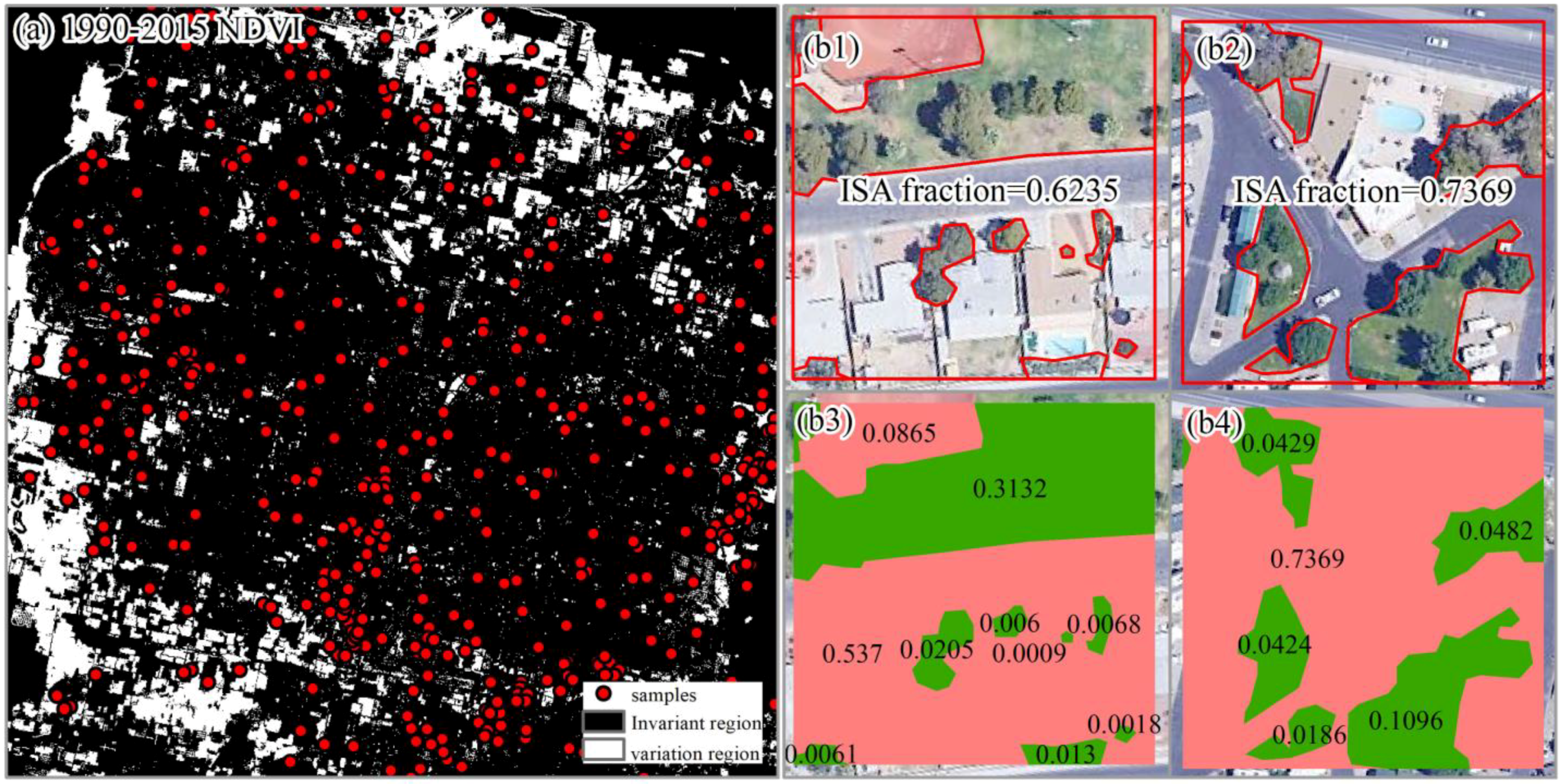
2.2.4. Accuracy Assessment

The accuracies of urban boundaries classification, the percentage of ISA, and GS fractions were assessed considering the principle and method of hierarchical architecture and subpixel metric of global urban land [56]. Globally, a total of 37,962 samples from different urban ecoregions along urban–rural gradients with a random sampling method were acquired within the sampled cities (Figure 4). The urban and non-urban land types were manually digitized based on Google Earth and GF-2 images in 2015 and circa 2020. The overall accuracy, producer’s accuracy, user’s accuracy, and Kappa coefficient were calculated to evaluate the accuracy of the urban boundaries map [40,57].
In terms of ISA and GS fractions, the 14,986 samples located in built-up areas using a stratified random sampling method with 10% intervals of the ISA fraction were acquired from global urban ecoregions. In those samples, the validation values of ISA and GS fractions with 3 × 3 pixels (90 m × 90 m) were calculated via manual digitalization derived from Google Earth images and GF-2 images [38,40]. The correlation coefficient (R) and root mean square error (RMSE) of ISA and GS fractions were calculated at global and continent scales. The above methods are explained in detail in previous publications [13,38,40,57]. R values were between 0.91 and 0.94, and RMSE values were between 0.03 and 0.18.

3. Results

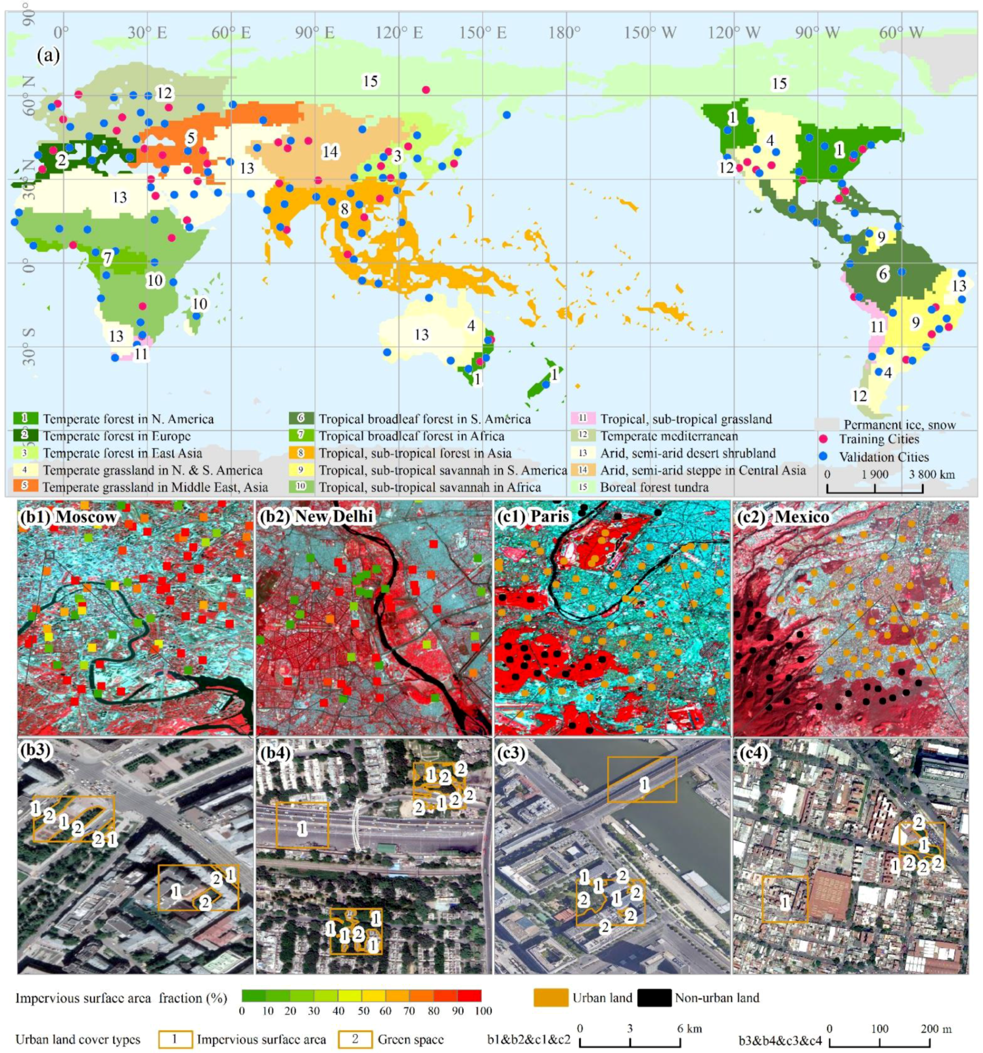
3.1. Performance and Accuracy of Ubran ISA and GS Fractions

Our assessment showed that the product has accurate urban boundaries and good performance in urban ISA and GS measures. The overall accuracies of the global urban boundaries are 91.40% and 91.63% for 2015 and circa 2020, respectively, and kappa coefficients are 0.870 and 0.860 for the same years (Table 2). However, the accuracies of urban boundaries among the continents illustrate the given discrepancies. In Europe, North America, South America, Asia and Oceania, the urban boundary maps have excellent overall accuracies of 91.10%, 92.10%, 92.31%, 91.58%, and 91.44% and kappa coefficients of 0.822, 0.842, 0.864, 0.832, and 0.857, respectively, the urban–rural boundaries were sharply segmented in the differential landscape and spatial configurations.
We also found that the maps of cities in Africa have slightly lower overall accuracies of 90.80% and kappa coefficients of 0.849 circa 2020 (Table 2). In North America, especially in the USA with its high urbanization, the cities are sprawling with low density in residential areas, and the spatial extents of cities are elongated well beyond the suburbs. Since the NSDI threshold in North America is relatively low at 40%, some areas of selected cities less than this threshold might not have been observed in the urban boundaries mapping. The lowest accuracies occur in arid and semi-arid cities in Africa and Oceania (Table 3). The landscapes in those cities are usually mosaicked with BS and built-up areas and are not differentiated from outlying areas.
The R and RMSE were used to assess the accuracy of ISA and GS fractions. The Rs of the global ISA and GS in 2015 were 0.93 and 0.92, and RMSEs were 0.13 and 0.14, respectively; circa 2020, Rs were 0.94 and 0.93, and RMSEs were 0.11 and 0.12, respectively (Table 3).

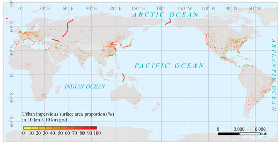
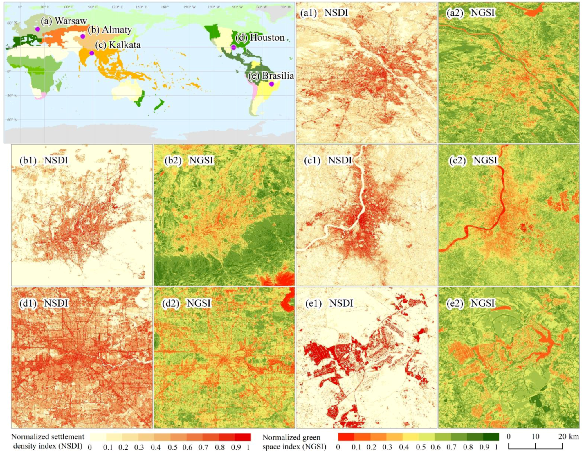
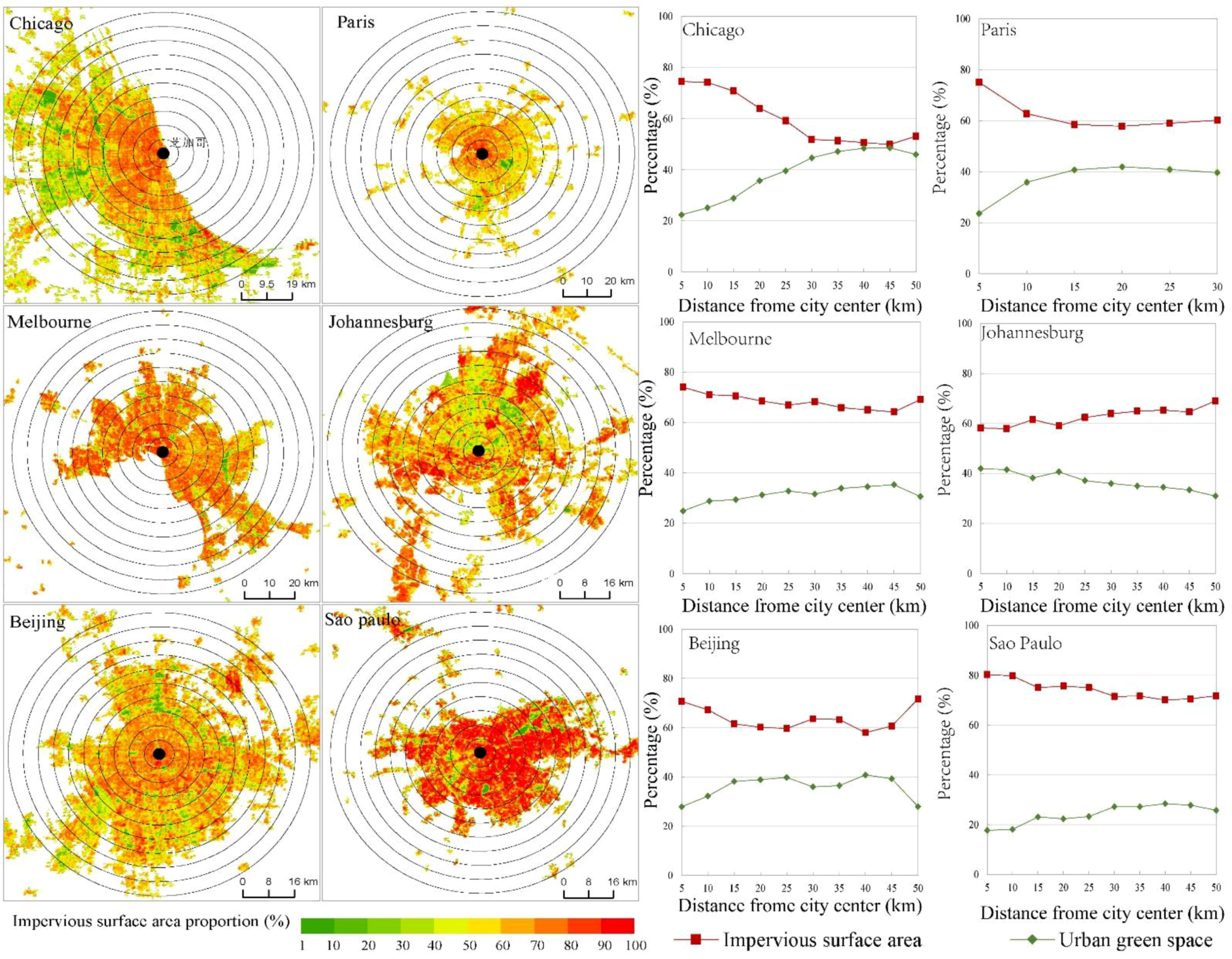
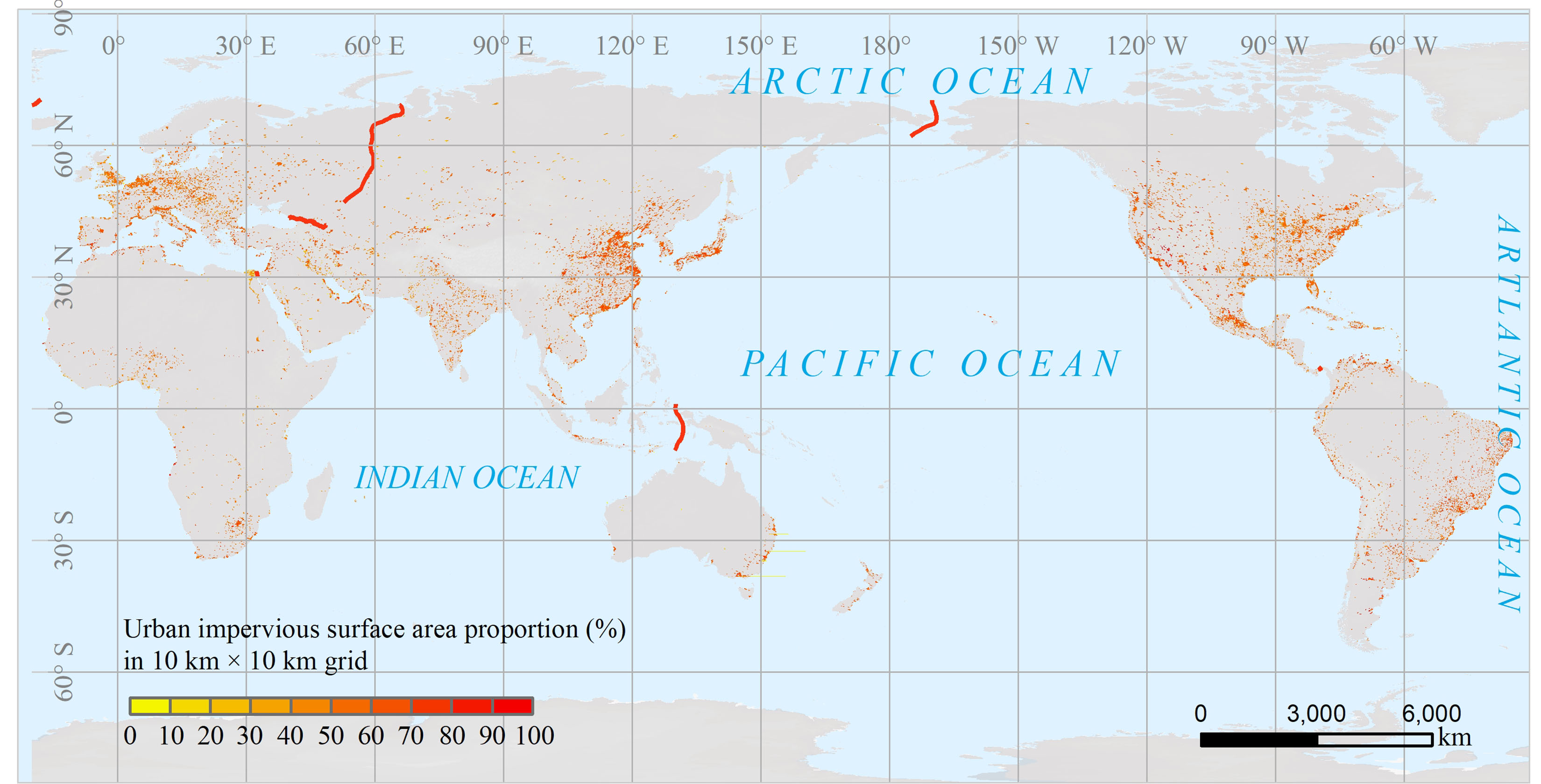
3.2. Distribution and Spatial Heterogenity of Global Urban ISA and GS

The global urban areas of ISA were 25.94 × 10⁴ km2 and 31.19 × 10⁴ km2 in 2015 and circa 2020, and GS areas were 13.46 × 10⁴ km2 and 17.16 × 10⁴ km2 in the same years. The percentages of ISA and GS in built-up areas averaged 62.34% and 32.35%, respectively, in 2015 and 60.00% and 33.00% circa 2020. Globally, 94.25% of pixels in built-up areas were between 10% and 90% ISA circa 2020, which exhibits the mosaicked patterns in intra-urban land cover (Figure 7).
The datasets reveal the large divergences of intra-urban ISA density and greening condition under different urban planning. Among the countries in Europe and some cities in the USA, the GS percentage is relatively high compared to other countries. For example, the ISA percentage of commercial zones in Chicago is approximately 70–80%, whereas it is less than 50% in residential areas along the fringes of the urban–rural gradient (Figure 8). The ISA and GS fractions in Chicago are 58.89% and 38.07%, respectively. However, ISAs of cities in Asia, Africa, and South America are relatively high. For example, the ISA and GS fractions in Delhi are 64.39% and 28.21%, respectively, due to high-density construction (Figure 8). We also examined some slum areas in Africa that lack city infrastructure and urban greening, in which the percentage of ISA is 80–90%. São Paulo exhibits ISA density of 80.95%, induced by the dense building layout (Figure 8).

3.3. Comparison with Other Existing Datasets

We compared the total areas, spatial configurations, and heterogeneity properties of global urban land from several mainstream datasets. Our estimation indicated large disparities among those datasets (Figure 9). A few datasets with 250 m to 1 km resolution (e.g., MODIS, DMSP/OLS) showed the extent of global urban land area as 24.47 × 10⁴–34.27 × 10⁴ km2 in the 1990s, 57.97 × 10⁴–65.70 × 10⁴ km2 in the 2000s, and 62.11 × 10⁴–78.97 × 10⁴ km2 in the 2010s [13,17,18,19,20,21]. We also examined several outcomes from research conducted at 30 m resolution, with global artificial cover at 118.75 × 10⁴ km2 in 2010 [24], global ISA at 74.71 ± 1.5 km2 in 2010 [25], global artificial impervious area (GAIA) at 79.71 × 10⁴ km2 in 2018 [9], and global urban boundaries at 80.97 × 10⁴ km2 in 2018 [28]. We determined that these differences are caused by incongruous definitions or concepts of spatial domains (Table S1).
Artificial settlements were categorized by three types, including urban land, rural settlements and industrial, or traffic lands in peripheries of cities [49]. However, urban extent was not often clearly defined in these earlier studies [9,21,25,28]. For example, the definition of ISA as built-up area usually included ISA in urban and rural settlements. As a result, some rural settlements are not excluded from spatial extents of urban land [25]. GAIA data covered ISA spatial extent in urban areas, some rural settlements, and industrial and traffic lands in suburban areas, which yield larger ISA than other research results [9]. Therefore, the disparate concepts of urban spatial domain may be the cause of the large divergences in global estimations of urban land area.
The issues of concept confusion, mixed pixels, and changing detection are intrinsically challenging for global mapping of urban land. In spatial extent, artificial ISA includes urban and rural settlements and industrial/traffic lands [9,24,25]. Nevertheless, in this concept, ISA is recorded as a single type, which cannot decompose mixed pixels into ISA and GS or other types of land cover [38,40]. Additionally, not extracting the minor percent of ISA in rural settlements from satellite images results in false estimates of actual urban extent. The different concepts of urban extent or the issues of mixed ISA pixels might result in overestimation of global urban ISA. Therefore, efforts to eliminate the uncertainties in area statistics of global urban land and delineate the underlying features of cities are emerging in existing global datasets [40].

4. Discussion

4.1. Advantages of the Methods and Algorithms Used to Map Urban ISA and GS Products

Considering the uncertainties of global urban land mapping, we developed a novel hierarchical architecture principle and subpixel method to address the issues of concept confusion and mixed pixels. Here, we segmented the urban land, rural settlements, and industrial and traffic lands at the peripheries of cities with thresholds to clarify the extent of urban land. A reasonable threshold of retrieval of global urban boundaries is essential due to the large divergences in social–economic levels, vegetation cover, and land-use intensity. In this procedure, the specific strategies are different, such as the kernel density approach and cellular automata model [27], the quantile-based digital number threshold identification [20], and the acquisition of centroid and threshold sites from normalized difference water, vegetation, and built-up indexes [25].
Although these methods could effectively identify urban extents or built-up areas, we examined the associated datasets and found some disadvantages in generating finer and more accurate urban boundaries retrieved from Landsat images. The quantile-based approach and kernel density approach might overgeneralize the urban boundaries, which could potentially generate a coarse spatial extent of built-up areas or cities [20,25]. Therefore, we adopted the best thresholds to acquire finer urban boundaries from the various urban ecoregions. In addition, the polygons of cities calibrated one at a time can effectively enhance the accuracy of urban boundaries.
Our estimation indicated that 67.41% of global urban land pixels are mosaicked with ISA and GS. The percentages of ISA and GS fractions based on the subpixel method produce accurate delineation of the spatial heterogeneity of urban underlying environments. Consequently, the definition and accurate metric of urban boundaries and mixed pixels were addressed to map the robust and reliable product.

4.2. Potential Implications for Improving Urban Environments and Assessments of Sustainable Cities

The urban ISA and GS fractions may effectively delineate the built-up environment of global cities based on our hierarchical architecture principle and subpixel method. Due to the high producer’s accuracy of 93.65% in the segmentation of urban–rural boundaries and the accurate and timely metrics of surface imperviousness and greening, our product has broad practical implications among the datasets [13]. Based on the product of urban ISA and GS fractions, the hotspot areas of dense ISA distribution may be identified by calculating the ISA density and growth intensification. Therefore, the thermal-dissipating strength of urban forest canopies and lawns may be assessed at pixel scale, and greening projects can more effectively address and alleviate urban heat island intensity [7]. Meanwhile, the intra-urban ISA and GS fractions can help identify flood regulation priority areas based on an ecosystem services approach [12].
Our assessment indicated global average urban land area per capita and percentage of ISA are 117.16 m2 and 60%, respectively, and the percentage of GS and GS area per capita are 33% and 41.29 m2. We also found large divergences between ISA density and greening levels among countries. As a result, urban planning and management in countries with high ISA densities and low greening levels are seriously challenged in addressing climate change and achieving SDGs [58,59,60]. Furthermore, our product will help in detailed assessments of progress toward SDG targets, such as the ratio of land consumption rate to population growth rate, and average share of the built-up area of cities that is open space for public use. Such systemic and detailed datasets can help create more knowledge about habitat environments and ecosystem services and improve global urban science [4].

5. Conclusions

In this research, a set of synthetic methodologies and technologies for depicting the urban land surface property were developed. We also confirmed that the hierarchical scale principle and subpixel method perform well in acquiring urban boundaries, as well as ISA and GS fractions. Our dataset has advantages of high accuracy in identifying the ISA and GS fractions in 30 m × 30 m pixels, and higher-resolution images were adopted to retrieve the urban extent or ISA with less than 30 m resolution compared to other datasets. The spatial heterogeneity of intra-urban land cover can be delineated with ISA and GS fractions at 30 m resolution. The product of urban ISA and GS fractions can be beneficial to urban planning and management, climate and ecology modeling, and assessments of the sustainable development of cities.

Supplementary Materials

The following are available online at https://www.mdpi.com/article/10.3390/rs13204187/s1, Table S1: A summary of global urban land-cover datasets, Table S2: The thresholds for mapping urban boundaries in each urban ecoregion, Table S3: The values of NDVIveg, NDVIsoil, β, and ISA and GS fractions in each urban ecoregion.

Author Contributions

Conceptualization, W.K.; data curation, Y.H. and W.K.; methodology, D.L. and W.K.; validation, Y.H., Y.D. and S.Y.; writing—original draft preparation, W.K., D.L., Y.D. and Y.H.; writing—review and editing, W.K., Y.H., Y.D., D.L. and S.Y.; project administration, W.K.; funding acquisition, W.K. All authors have read and agreed to the published version of the manuscript.

Funding

This research was supported by the Strategic Priority Research Program of Chinese Academy of Sciences, Pan-Third Pole Environment Study for a Green Silk Road (Pan-TPE) (XDA20040400); National Natural Science Foundation of China, grant number 41871343.

Institutional Review Board Statement

Not applicable.

Informed Consent Statement

Not applicable.

Data Availability Statement

Not applicable.

Acknowledgments

Many thanks to the anonymous reviewers and the editor for providing valuable opinions for revising the manuscript.

Conflicts of Interest

The authors declare no conflict of interest.

References

  1. Grimm, N.B.; Faeth, S.H.; Golubiewski, N.E.; Redman, C.L.; Wu, J.; Bai, X.; Briggs, J.M. Global change and the ecology of cities. Science 2008, 319, 756–760. [Google Scholar] [CrossRef] [PubMed] [Green Version]
  2. Gao, J.; O’Neill, B.C. Mapping global urban land for the 21st century with data-driven simulations and shared socioeconomic pathways. Nat. Commun. 2020, 11, 2302. [Google Scholar] [CrossRef] [PubMed]
  3. Seto, K.C.; Golden, J.S.; Alberti, M.; Turner, B.L., II. Sustainability in an urbanizing planet. Proc. Natl. Acad. Sci. USA 2017, 114, 8935–8938. [Google Scholar] [CrossRef] [PubMed] [Green Version]
  4. Acuto, M.; Parnell, S.; Seto, K.C. Building a global urban science. Nat. Sustain. 2018, 1, 2–4. [Google Scholar] [CrossRef]
  5. Turner, B.L., II. Land system architecture for urban sustainability: New directions for land system science illustrated by application to the urban heat island problem. J. Land Use Sci. 2016, 11, 689–697. [Google Scholar] [CrossRef]
  6. Jacobson, C.R. Identification and quantification of the hydrological impacts of imperviousness in urban catchments: A review. J. Environ. Manag. 2011, 92, 1438–1448. [Google Scholar] [CrossRef] [PubMed]
  7. Kuang, W.H.; Dou, Y.Y.; Zhang, C.; Chi, W.F.; Liu, A.L.; Liu, Y.; Zhang, R.H.; Liu, J.Y. Quantifying the heat flux regulation of metropolitan land use/land cover components by coupling remote sensing modeling with in situ measurement. J. Geophys. Res.-Atmos. 2015, 120, 113–130. [Google Scholar] [CrossRef]
  8. Yan, Y.; Kuang, W.H.; Zhang, C.; Chen, C.B. Impacts of impervious surface expansion on soil organic carbon: A spatially explicit study. Sci. Rep. 2015, 5, 17905. [Google Scholar] [CrossRef] [Green Version]
  9. Gong, P.; Li, X.C.; Wang, J.; Bai, Y.; Chen, B.; Hu, T.; Liu, X.; Xu, B.; Yang, J.; Zhang, W.; et al. Annual maps of global artificial impervious area (GAIA) between 1985 and 2018. Remote Sens. Environ. 2020, 236, 111510. [Google Scholar] [CrossRef]
  10. Seto, K.C.; Guneralp, B.; Hutyra, L.R. Global forecasts of urban expansion to 2030 and direct impacts on biodiversity and carbon pools. Proc. Natl. Acad. Sci. USA 2012, 109, 16083–16088. [Google Scholar] [CrossRef] [Green Version]
  11. Bren d’Amour, C.; Reitsma, F.; Baiocchi, G.; Barthel, S.; Güneralp, B.; Erb, K.-H.; Haberl, H.; Creutzig, F.; Seto, K.C. Future urban land expansion and implications for global croplands. Proc. Natl. Acad. Sci. USA 2017, 114, 8939–8944. [Google Scholar] [CrossRef] [PubMed] [Green Version]
  12. Li, X.Y.; Kuang, W.H.; Sun, F.Y. Identifying urban flood regulation priority areas in Beijing based on an ecosystem services approach. Sustainability 2020, 12, 2297. [Google Scholar] [CrossRef] [Green Version]
  13. Kuang, W.H. Mapping global impervious surface area and green space within urban environments. Sci. China Earth Sci. 2019, 62, 1591–1606. [Google Scholar] [CrossRef]
  14. Dong, J.W.; Kuang, W.H.; Liu, J.Y. Continuous land cover change monitoring in the remote sensing big data era. Sci. China Earth Sci. 2017, 60, 2223–2224. [Google Scholar] [CrossRef]
  15. Feng, M.; Li, X. Land cover mapping toward finer scales. Sci. Bull. 2020, 65, 1604–1606. [Google Scholar] [CrossRef]
  16. Gong, J.; Liu, C.; Huang, X. Advances in urban information extraction from high-resolution remote sensing imagery. Sci. China Earth Sci. 2020, 63, 463–475. [Google Scholar] [CrossRef]
  17. Elvidge, C.D.; Tuttle, B.T.; Sutton, P.S.; Baugh, K.E.; Howard, A.T.; Milesi, C.; Bhaduri, B.L.; Nemani, R. Global distribution and density of constructed impervious surfaces. Sensors 2007, 7, 1962–1979. [Google Scholar] [CrossRef]
  18. Schneider, A.; Friedl, M.A.; Potere, D. A new map of global urban extent from MODIS satellite data. Environ. Res. Lett. 2009, 4, 044003. [Google Scholar] [CrossRef] [Green Version]
  19. Schneider, A.; Friedl, M.A.; Potere, D. Mapping global urban areas using MODIS 500 m data: New methods and datasets based on “urban ecoregions”. Remote Sens. Environ. 2010, 114, 1733–1746. [Google Scholar] [CrossRef]
  20. Zhou, Y.Y.; Li, X.C.; Asrar, G.R.; Smith, S.J.; Imhoff, M. A global record of annual urban dynamics (1992–2013) from nighttime lights. Remote Sens. Environ. 2018, 219, 206–220. [Google Scholar] [CrossRef]
  21. He, C.Y.; Liu, Z.F.; Gou, S.Y.; Zhang, Q.F.; Zhang, J.S.; Xu, L.L. Detecting global urban expansion over the last three decades using a fully convolutional network. Environ. Res. Lett. 2019, 14, 034008. [Google Scholar] [CrossRef]
  22. Esch, T.; Marconcini, M.; Felbier, A.; Roth, A.; Heldens, W.; Huber, M.; Schwinger, M.; Taubenböck, H.; Müller, A.; Dech, S. Urban footprint processor—Fully automated processing chain generating settlement masks from global data of the TanDEM-X mission. IEEE Geosci. Remote Sens. Lett. 2013, 10, 1617–1621. [Google Scholar] [CrossRef] [Green Version]
  23. Pesaresi, M.; Huadong, G.; Blaes, X.; Ehrlich, D.; Ferri, S.; Gueguen, L.; Halkia, M.; Kauffmann, M.; Kemper, T.; Lu, L.; et al. A global human settlement layer from optical HR/VHR RS data: Concept and first results. IEEE J. Sel. Top. Appl. Earth Obs. Remote Sens. 2013, 6, 2102–2131. [Google Scholar] [CrossRef]
  24. Chen, J.; Chen, J.; Liao, A.P.; Cao, X.; Chen, L.J.; Chen, X.H.; He, C.Y.; Han, G.; Peng, S.; Lu, M.; et al. Global land cover mapping at 30 m resolution: A POK-based operational approach. ISPRS J. Photogramm. 2015, 103, 7–27. [Google Scholar] [CrossRef] [Green Version]
  25. Liu, X.P.; Hu, G.H.; Chen, Y.M.; Li, X.; Xu, X.C.; Li, S.Y.; Pei, F.S.; Wang, S.J. High-resolution multi-temporal mapping of global urban land using Landsat images based on the Google Earth Engine Platform. Remote Sens. Environ. 2018, 209, 227–239. [Google Scholar] [CrossRef]
  26. Liu, X.P.; Huang, Y.H.; Xu, X.C.; Li, X.C.; Li, X.; Ciais, P.; Lin, P.R.; Gong, K.; Ziegler, A.D.; Chen, A.P.; et al. High-spatiotemporal-resolution mapping of global urban change from 1985 to 2015. Nat. Sustain. 2020, 3, 564–570. [Google Scholar] [CrossRef]
  27. Zhang, X.; Liu, L.Y.; Wu, C.S.; Chen, X.D.; Gao, Y.; Xie, S.; Zhang, B. Development of a global 30 m impervious surface map using multisource and multitemporal remote sensing datasets with the Google Earth Engine platform. Earth Syst. Sci. Data 2020, 12, 1625–1648. [Google Scholar] [CrossRef]
  28. Li, X.C.; Gong, P.; Zhou, Y.Y.; Wang, J.; Bai, Y.Q.; Chen, B.; Hu, T.; Xiao, Y.X.; Xu, B.; Yang, J.; et al. Mapping global urban boundaries from the global artificial impervious area (GAIA) data. Environ. Res. Lett. 2020, 15, 094044. [Google Scholar] [CrossRef]
  29. Wang, P.S.; Huang, C.Q.; Brown de Colstoun, E.C.; Tilton, J.C.; Tan, B. Global Human Built-Up and Settlement Extent (HBASE) Dataset from Landsat; NASA Socioeconomic Data and Applications Center (SEDAC): Palisades, NY, USA, 2017. [Google Scholar] [CrossRef]
  30. Ludwig, C.; Hecht, R.; Lautenbach, S.; Schorcht, M.; Zipf, A. Mapping public urban green spaces based on OpenStreetMap and Sentinel-2 imagery using belief functions. ISPRS Int. J. Geo-Inf. 2021, 10, 251. [Google Scholar] [CrossRef]
  31. Bossard, M.; Feranec, J.; Otahel, J. CORINE Land Cover Technical Guide: Addendum 2000; European Environment Agency: Copenhagen, Denmark, 2000. [Google Scholar]
  32. Seifert, F.M. Improving urban monitoring toward a European urban atlas. In Global Mapping of Human Settlement: Experiences, Datasets, and Prospects; CRC Press: Boca Raton, FL, USA, 2009; pp. 231–248. [Google Scholar]
  33. The Trust for Public Land. Available online: https://www.tpl.org/parkserve (accessed on 12 April 2021).
  34. Feltynowski, M.; Kronenberg, J.; Bergier, T.; Kabisch, N.; Laszkiewicz, E.; Stronhbach, M.W. Challenges of urban green space management in the face of using inadequate data. Urban For. Urban Green. 2018, 31, 56–66. [Google Scholar] [CrossRef]
  35. Tigges, J.; Lakes, T.; Hostert, P. Urban vegetation classification: Benefits of multitemporal RapidEye satellite data. Remote Sens. Environ. 2013, 136, 66–75. [Google Scholar] [CrossRef]
  36. Lu, D.S.; Moran, E.; Hetrick, S. Detection of impervious surface change with multitemporal Landsat images in an urban-rural frontier. ISPRS J. Photogramm. 2011, 66, 298–306. [Google Scholar] [CrossRef] [PubMed] [Green Version]
  37. Reba, M.; Seto, K. A systematic review and assessment of algorithms to detect, characterize, and monitor urban land change. Remote Sens. Environ. 2020, 242, 111739. [Google Scholar] [CrossRef]
  38. Kuang, W.H.; Chi, W.F.; Lu, D.S.; Dou, Y.Y. A comparative analysis of megacity expansions in China and the U.S.: Patterns, rates and driving forces. Landsc. Urban Plan. 2014, 132, 121–135. [Google Scholar] [CrossRef]
  39. Kuang, W.H.; Yang, T.R.; Liu, A.L.; Zhang, C.; Lu, D.S.; Chi, W.F. An EcoCity model for regulating urban land cover structure and thermal environment: Taking Beijing as an example. Sci. China Ser. D-Earth Sci. 2017, 60, 1098–1109. [Google Scholar] [CrossRef]
  40. Kuang, W.H. National urban land-use/cover change since the beginning of the 21st century and its policy implications in China. Land Use Policy 2020, 97, 104747. [Google Scholar] [CrossRef]
  41. Walton, J.T. Subpixel urban land cover estimation: Comparing cubist, random forests, and support vector regression. Photogramm. Eng. Remote Sens. 2008, 10, 1213–1222. [Google Scholar] [CrossRef] [Green Version]
  42. Reschke, J.; Hüttich, C. Continuous field mapping of Mediterranean wetlands using sub-pixel spectral signatures and multi-temporal Landsat data. Int. J. Appl. Earth Obs. 2014, 28, 220–229. [Google Scholar] [CrossRef]
  43. Huang, X.; Schneider, A.; Friedl, M. A Mapping sub-pixel urban expansion in China using MODIS and DMSP/OLS nighttime lights. Remote Sens. Environ. 2016, 175, 92–108. [Google Scholar] [CrossRef]
  44. Tsutsumida, N.; Comber, A.; Barrett, K.; Saizen, I.; Rustiadi, E. Sub-pixel classification of MODIS EVI for annual mappings of impervious surface areas. Remote Sens. 2016, 8, 143. [Google Scholar] [CrossRef] [Green Version]
  45. Zhao, Y.; Zhong, K.W.; Xu, J.H.; Sun, C.; Wang, Y.P. Directional analysis of urban expansion based on sub-pixel and regional scale: A case study of main districts in Guangzhou, China. Chin. Geogr. Sci. 2019, 29, 652–666. [Google Scholar] [CrossRef] [Green Version]
  46. Li, L.Y.; Chen, Y.; Xu, T.B.; Meng, L.K.; Huang, C.; Shi, K.F. Spatial Attraction Models Coupled with Elman Neural Networks for Enhancing Sub-Pixel Urban Inundation Mapping. Remote Sens. 2020, 13, 2068. [Google Scholar] [CrossRef]
  47. Patidar, N.; Keshari, A.K. A rule-based spectral unmixing algorithm for extracting annual time series of sub-pixel impervious surface fraction. Int. J. Remote Sens. 2020, 10, 3970–3992. [Google Scholar] [CrossRef]
  48. Xian, G.; Shi, H.; Dewitz, J.; Wu, Z.T. Performances of WorldView 3, Sentinel 2, and Landsat 8 data in mapping impervious surface. Remote Sens. Appl. Soc. Environ. 2019, 15, 100246. [Google Scholar] [CrossRef]
  49. Liu, J.Y.; Kuang, W.H.; Zhang, Z.X.; Xu, X.L.; Qin, Y.W.; Ning, J.; Zhou, W.C.; Zhang, S.W.; Li, R.D.; Yan, C.Z.; et al. Spatiotemporal characteristics, patterns, and causes of land-use changes in China since the late 1980s. J. Geogr. Sci. 2014, 24, 195–210. [Google Scholar] [CrossRef]
  50. Chan, C.W.; Paelinckx, D. Evaluation of random forest and Adaboost tree-based ensemble classification and spectral band selection for ecotope mapping using airborne hyperspectral imagery. Remote Sens. Environ. 2008, 112, 2999–3011. [Google Scholar] [CrossRef]
  51. Brown de Colstoun, E.C.; Huang, C.; Wang, P.; Tilton, J.C.; Tan, B.; Phillips, J.; Niemczura, S.; Ling, P.Y.; Wolfe, R.E. Global Man-Made Impervious Surface (GMIS) Dataset from Landsat; NASA Socioeconomic Data and Applications Center (SEDAC): Palisades, NY, USA, 2017. [Google Scholar] [CrossRef]
  52. Goldblatt, R.; Stuhlmacher, M.F.; Tellman, B.; Clinton, N.; Hanson, G.; Georgescu, M.; Wang, C.; Serrano-Candela, F.; Khan-Delwal, A.K.; Cheng, W.H.; et al. Using Landsatand nighttime lights for supervised pixel-based image classification of urban land cover. Remote Sens. Environ. 2018, 205, 253–275. [Google Scholar] [CrossRef]
  53. Gislason, P.O.; Benediktsson, J.A.; Sveinsson, J.R. Random forests for land cover classification. Pattern Recogn. Lett. 2006, 27, 294–300. [Google Scholar] [CrossRef]
  54. Pekel, J.F.; Cottam, A.; Gorelick, N.; Belward, A.S. High-resolution mapping of global surface water and its long-term changes. Nature 2016, 540, 418–422. [Google Scholar] [CrossRef]
  55. As-Syakur, A.R.; Adnyana, I.W.S.; Arthana, I.W.; Nuarsa, I.W. Enhanced built-up and bareness index (EBBI) for mapping built-up and bare land in an urban area. Remote Sens. 2012, 4, 2957–2970. [Google Scholar] [CrossRef] [Green Version]
  56. Kuang, W.H.; Du, G.M.; Lu, D.S.; Dou, Y.Y.; Li, X.Y.; Zhang, S.; Chi, W.F.; Dong, J.W.; Chen, G.S.; Yin, Z.R.; et al. Global observation of urban expansion and land-cover dynamics using satellite big-data. Sci. Bull. 2020, 66, 297–300. [Google Scholar] [CrossRef]
  57. Kuang, W.H.; Liu, J.Y.; Dong, J.W.; Chi, W.F.; Zhang, C. The rapid and massive urban and industrial land expansions in China between 1990 and 2010: A CLUD-based analysis of their trajectories, patterns, and drivers. Landsc. Urban Plan. 2016, 145, 21–33. [Google Scholar] [CrossRef]
  58. Bierwagen, B.G.; Theobald, D.M.; Pyke, C.R.; Choate, A.; Groth, P.; Thomas, J.V.; Morefield, P. National housing and impervious surface scenarios for integrated climate impact assessments. Proc. Natl. Acad. Sci. USA 2010, 107, 20887–20892. [Google Scholar] [CrossRef] [PubMed] [Green Version]
  59. Pataki, D.E. Urban greening needs better data. Nature 2013, 502, 624. [Google Scholar] [CrossRef] [Green Version]
  60. Georgescu, M.; Morefield, P.E.; Bierwagen, B.G.; Weaver, C.P. Urban adaptation can roll back warming of emerging megapolitan regions. Proc. Natl. Acad. Sci. USA 2014, 111, 2909–2914. [Google Scholar] [CrossRef] [Green Version]
Figure 1. The hierarchical scale principle and subpixel metric method for mapping ISA and GS fractions.
Remotesensing 13 04187 g001
Figure 2. The strategy for mapping urban impervious surface area (ISA) and green space (GS) products (NSDI, Normalized Settlement Density Index; NGSI, Normalized Green Space Index).
Remotesensing 13 04187 g002
Figure 3. (a) shows the selection principle of the spatial distribution of sample points; (b1,b2) show the sampling areas in a Google Earth image; whereas (b3,b4) show the digitized proportions of the impervious (pink) and vegetation (green) areas.
Remotesensing 13 04187 g003
Figure 4. (a) shows the distribution of global urban ecoregions and sampled cities; (b1,b2) show the impervious surface area fraction in sampled cities; (c1,c2) show the urban and non-urban land in sampled cities; (b3,b4,c3,c4) show the digitized the impervious and vegetation areas.
Remotesensing 13 04187 g004
Figure 5. Examples of spatial distribution of NSDI and NGSI in selected regions circa 2020. (a1,b1,c1,d1,e1) show the NSDI in selected regions; (a2,b2,c2,d2,e2) show the NGSI in selected regions.
Remotesensing 13 04187 g005
Figure 6. Examples of urban impervious surface area fraction in selected cities. (a1,b1,c1,d1,e1) show the urban impervious surface area fraction in 2005; (a2,b2,c2,d2,e2) show the urban impervious surface area fraction circa 2020.
Remotesensing 13 04187 g006
Figure 7. Spatial distribution of global ISA (a1) and GS (a2) circa 2020. (b1,c1,d1,e1,f1,g1) show the areas of ISA in different regions; (b2,c2,d2,e2,f2,g2) show the areas of GS in different regions.
Remotesensing 13 04187 g007
Figure 8. The percentages of impervious surface areas and green spaces in urban land areas in selected cities.
Remotesensing 13 04187 g008
Figure 9. Comparisons between our dataset and other existing datasets. (GUE, global urban expansion [21]; GUL, global urban land [25]; GHSL, global human settlement layer [23]; GAIA, global artificial impervious area [9]; and MSMT, global ISA [27]).
Remotesensing 13 04187 g009
Table 1. The data sources for mapping urban impervious surface area and green space products.
Data SourceResolutionScene/ExtentCovered Period
Landsat 8 OLI30 m/15 m146,8781 January 2015–31 December 2015
Landsat 8 OLI30 m/15 m160,6591 February 2019–31 January 2020
SRTM Digital Elevation30 mGlobal--
Google Earth images0.6 m8652015 and circa 2020
Gaofen-2 (GF-2)4 m/1 m536Circa 2020
Global surface water30 mGlobal2015 and circa 2020
DMSP/OLS1 km/500 mGlobal2015 and circa 2020
Table 2. The accuracy of urban boundaries acquired from Landsat images in 2015 and circa 2020.
2015Circa 2020
IndexPA (%)UA (%)OA (%)KappaPA (%)UA (%)OA (%)Kappa
Asia90.1990.5890.380.90091.1991.9891.580.832
Europe91.2293.1092.150.92690.5691.6491.100.822
North America91.3392.4091.860.83791.6092.6092.100.842
South America91.3092.8492.070.86891.4593.1992.310.864
Africa90.2091.9291.050.85590.4991.1290.800.849
Oceania91.1591.6291.380.86491.0391.8691.440.857
Global90.7892.0391.400.87091.1192.1591.630.860
Table 3. The accuracy of urban impervious surface area (ISA) and green space (GS) fractions acquired from Landsat images in 2015 and circa 2020.
2015Circa 2020
Data TypeISAGSISAGS
IndexRRMSERRMSERRMSERRMSE
Asia0.930.140.930.140.940.120.930.11
Europe0.930.160.930.130.940.150.940.16
North America0.940.130.930.140.940.130.920.14
South America0.930.030.920.080.930.030.930.11
Africa0.920.150.910.180.920.130.910.12
Oceania0.930.140.920.150.940.080.920.10
Global0.930.130.920.140.940.110.930.12
Publisher’s Note: MDPI stays neutral with regard to jurisdictional claims in published maps and institutional affiliations.

