Article

Assessing Community-Level Livability Using Combined Remote Sensing and Internet-Based Big Geospatial Data

1
Shandong Provincial Key Laboratory of Water and Soil Conservation and Environmental Protection, College of Resources and Environment, Linyi University, Linyi 276000, China
2
Key Laboratory of Earth Surface Processes of Ministry of Education, College of Urban and Environmental Sciences, Peking University, Beijing 100871, China
3
College of Applied Arts and Science, Beijing Union University, Beijing 100191, China
*
Author to whom correspondence should be addressed.
Remote Sens. 2020, 12(24), 4026; https://doi.org/10.3390/rs12244026
Submission received: 29 November 2020 / Revised: 8 December 2020 / Accepted: 8 December 2020 / Published: 9 December 2020

Abstract

:
With rapid urbanization, retrieving livability information of human settlements in time is essential for urban planning and governance. However, livability assessments are often limited by data availability and data update cycle, and this problem is more serious when making an assessment at finer spatial scales (e.g., community level). Here we aim to develop a reliable and dynamic model for community-level livability assessment taking Linyi city in Shandong Province, China as a case study. First, we constructed a hierarchical index system for livability assessment, and derived data for each index and community from remotely sensed data or Internet-based geospatial data. Next, we calculated the livability scores for all communities and assessed their uncertainties using Monte Carlo simulations. The results showed that the mean livability score of all communities was 59. The old urban and newly developed districts of our study area had the best livability, and got a livability score of 62 and 58 respectively, while industrial districts had the poorest conditions with an average livability score of 48. Results by dimension showed that the old urban district had better conditions of living amenity and travel convenience, but poorer conditions of environmental health and comfort. The newly developed districts were the opposite. We conclude that our model is effective and extendible for rapidly assessing community-level livability, which provides detailed and useful information of human settlements for sustainable urban planning and governance.

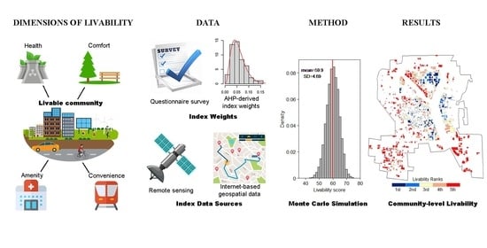
Graphical Abstract

1. Introduction

The physical extent of cities has grown at an accelerating rate over the past century, and more than 50% of the global population now lives in urban areas [1,2]. Dramatic population growth and resultant rapid urban expansion has driven socio-economic and environmental changes on multiple scales, including air pollution, urban heat island, the loss of biodiversity, and so forth, which, in turn, exerts profound effects on human living conditions [3,4]. Therefore, assessing how livability changes over time is the premise of making urban governance to address the negative effects of urbanization on human inhabitation [5]. Livability assessment is even more important in China, which is one of the fastest urbanizing countries and is being severely bothered by concerns of urbanization, such as air pollution, traffic congestion, and overcrowded population levels [6,7,8].
The livability assessment has been mainly conducted at three levels [9]. At the top level, the livability assessment is made by treating the city as a whole, and reveals the degree of livability and potential problems through comparison among cities [5,10,11,12]. The indices are often selected to reflect environmental, ecological, social, and economic attributes on the city-scale. This kind of assessment is helpful for making regional planning to build livable cities at broader scales, but is insufficient to support governance within the city [13,14]. At the bottom level, livability assessment focuses more on individual residence or even building, and thus the indices at the microscopic level are often selected, which includes floor area, story, sunshine duration, amenities, and so forth. Such an assessment is often made from the perspective of architecture, so it fails to take into account geographic context and location characteristics [15]. In contrast, at the middle level, livability assessments are made for spatial units within the city such as blocks, communities, and artificially delineated grids. It considers both local property information and environmental background on broader scales, which are able to truly reflect living environment of urban inhabitants [16,17,18]. Therefore, middle-level assessment (e.g., community-level) can provide detailed livability information that sufficiently supports urban planning and governance.
The use of different data sources has differentiated the methods into qualitative and quantitative livability assessments [9,13,19]. Questionnaire surveys of randomly selected communities and participatory interviews are two widely used ways to assess livability qualitatively [20,21,22,23]. These methods are effective to capture the perceptions and satisfaction of urban dwellers to their living environment, which is useful for understanding the evolution mechanisms of urban structure and their driving forces, and provides insights into human-oriented urban planning [23]. However, making interview and questionnaire surveys is time- and labor-intensive, rendering it difficult to update data and extensively conduct planning in multiple cities [16]. Moreover, the survey cannot cover all communities, and thus cannot meet the requirements of urban governance which often needs livability information as exhaustive as possible [13]. In comparison, GIS-based methods, which depend heavily on basic geographic information collected by government agencies [19], can provide livability information for all communities to overcome the limitations of questionnaire surveys. However, the approach is not suitable for dynamic assessment given that the input geographic information often updates slowly. Therefore, a model that is suitable for dynamic assessment and whose inputs are readily acquired is needed to provide sufficient support for urban governance.
Rapid development of remote sensing and big geospatial data technology has substantially improved our understanding of cities, and has helped us explore more deeply urban lifestyles and urban function patterns [7,24]. Key attributes of living environment such as urban land cover patterns, thermal conditions, and air pollution are able to be effectively retrieved from remotely sensed imagery [25,26]. Big data, such as mobile signaling, social media data, point of interest (POI), and algorithm-based online platforms, have been mined to extract information about human behaviors, population density and migration, transportation, urban infrastructure, function of land use, etc., which are closely related to our living environment [27]. Therefore, remotely sensed imagery and big geospatial data are desirable data sources of livability assessment due to their easy availability, repeatable observations or collections, and broad-scale coverage. Here our archiving goal is to develop an effective livability assessment model using combined remote sensing and Internet-based big geospatial data. We took Linyi city in the Shandong Province of China as the study area, within which the living environment was characterized by high spatial heterogeneity. First, we constructed a hierarchical index system for community livability, and derived the data of each index mainly from remote sensing and an Application Programming Interface (API) of the city’s big geospatial data. Then, we calculated the livability scores for all communities using the weighted sum method and Monte Carlo simulations, and generated the spatial pattern of livability for the city. Our research could showcase the use of remote sensing and big data technology for livability assessment, which provides an effective guide for urban governance.

2. Materials and Methods

2.1. Study Area

Linyi is the largest city in the southeast of Shandong Province of China, and the built-up area is made up of Lanshan District, Luozhuang District, and Hedong District (Figure 1). The urban area mostly lies on flat land, and has a warm temperate climate with warm, humid summers and cold, dry winters. Linyi has a heterogeneous landscape, with the industrial zones scattered in the west, southwest, and southeast, the old urban district, mainly commercial and residential, sits in the center, and the newly developed district is located in the north. Urban function patterns in our study area has evident spatial differentiation, which results in a highly heterogeneous living environment.
We chose community as the basic spatial unit for assessment, which resulted in 997 communities in the urban area of Linyi (Figure 1). For one thing, unlike countries such as the United States and Canada, the communities in China often take the form of a gated residential area with a clear boundary, so it is easy to identify them based on high-resolution imagery. For another, assessment at this finer scale allows for the development of locally specific regulations and policies. Accurate identification of the community extent is essential for reliable livability assessment. Up to now, manually delineating communities by experienced analysts was still the credible method to acquire the spatial extent of communities. To get the extent of the community, we retrieved POIs of all communities based on the Baidu Map place API (http://lbsyun.baidu.com/index.php?title=webapi/guide/webservice-placeapi), and input these POIs with geographical coordinates into ArcGIS software to generate a KML (Keyhole Markup Language) file. The KML file was overlapped onto the high-resolution Google Earth imagery, and the boundaries for all communities corresponding to the community POIs were manually digitalized.

2.2. Data

2.2.1. Remotely Sensed Data

We used the Sentinel-2A/B imagery to retrieve the land use map, which was needed to calculate data of some indices (e.g., green space). The European Space Agency launched two satellites of the Sentinel-2 missions (S-2A and S-2B respectively) in 2015 and 2017. The Multi-Spectral Instrument (MSI) sensors onboard both satellites provide a spatial resolution of 10 to 60 m depending on the wavelength: 10 m for the visible and the broad NIR bands, 20 m for the red edge, narrow NIR and SWIR bands, and 60 m for the atmospheric bands. The revisit frequency of each single Sentinel-2 satellite is 10 days, and two satellites can give a high revisit frequency of 5 days at the Equator. Therefore, the Sentinel-2 imagery with high spatial and temporal resolution has supported land cover mapping and vegetation growth monitoring [28]. Standard Sentinel-2 L1C data for the study area was obtained from the ESA Open Access Hub, which were framed into tiles (also named granules) measuring 109.8 km by 109.8 km in the UTM-based Military Grid Reference System.
We used the MODIS Version 6 Land Surface Temperature (LST) products from Terra and Aqua satellites (MOD11A1 and MYD11A1 respectively) to derive the duration of thermal comfort for each community. MODIS LST is estimated from two thermal infrared bands 31 (10.78–11.28 μm) and 32 (11.77–12.27 μm) using the generalized split-window algorithm [29]. The products provide daily per-pixel LST at 1 km spatial resolution in a 1200 by 1200 km tile. The daily LST data further includes two daytime observations (10:30 a.m. on Terra and 1:30 p.m. on Aqua in local time) and two nighttime observations (10:30 p.m. on Terra and 1:30 a.m. on Aqua in local time). MODIS LST has many advantages including high spatial and temporal resolution, global coverage and long-term observations, which makes it one of the most widely used LST products in characterizing urban heat island [25].

2.2.2. Internet-Based Geospatial Data

We mainly used the Web service Application Programming Interface (API) provided by the Baidu Map (http://lbsyun.baidu.com/) to extract the data of indices such as travel distance, traffic status, and POI. The Web service API provides an http/https interface so that the developers can initiate a search request through the http/https form to retrieve the data of many core services in json or xml format. For example, the route calculation service (RouteMatrix) API (http://lbsyun.baidu.com/index.php?title=webapi/route-matrix-api-v2) allows users to calculate the distance and travel time of an optimal route between the start and end points by different ways of transportation (driving, cycling, and walking).

2.3. Model Development

2.3.1. Procedures to Build Model

There were four procedures to be taken to develop the assessment model (Figure 2). First, we constructed a hierarchical index system for livability assessment through an extensive literature review, expert consulting, and analyzing geographical features of our study area. Second, we derived the data for each index using remote sensing and Internet-based geospatial techniques, and rescaled the data to make them comparable among different indices. Third, we determined the weights of indices using a questionnaire survey and the Analytic Hierarchy Process (AHP) method. Finally, the weighted sum method and Monte Carlo simulation was applied to calculate livability scores and their uncertainties of communities.

2.3.2. Constructing an Assessment Index System

We constructed a hierarchical index system for livability assessment through an extensive literature review and analyses of the geographical features of our study area. At the top level, we used a widely used framework to show the dimensions of livability assessment. This framework was put forward by the World Health Organization (WHO) in 1976, which had four dimensions including safety, health, convenience, and amenity [30]. Since then, researchers have further developed this framework and designed multi-dimensional hierarchical index systems to characterize urban livability [9,31]. For example, Zhang (2007) [9] summarized the potential factors that substantially impact livability, and classified them into five dimensions including safety, environmental health, living amenity, travel convenience, and environmental comfort. This five-dimensional framework has effectively guided the selection of indices, and then the design of an index system for livability assessment at both city and block levels [5,17,20,32]. Given the situations of our study area, assessment units, and data availability, we adopted this framework and selected indices from the dimensions of environmental health, environmental comfort, living amenity, and travel convenience at the top level (Table 1). At the bottom level, we selected 16 indices in total under different dimensions, which would exert a great influence on residents’ livability in our study area (Table 1). Below is the description of indices in detail.
Environmental health means that residents in a community are able to enjoy a healthy living environment [9]. A livable community should be characterized by fresh air condition, high water quality, mild climate, staying away from hazardous materials and environmental pollutants, and so forth [5,33,34]. Among them, urban heat island (UHI) has been a common phenomenon due to the particular characteristics of urban environment (i.e., increased impervious surfaces, decreased water surfaces, and green spaces), and the adverse effects have been well-documented, such as more frequent heat waves and increased heat-related mortality [3,25]. Our study area in the warm temperate climate zone suffers from frequent heat waves in summer, and the conditions deteriorate due to the effects of UHI. Therefore, we selected the index and the duration of thermal comfort to indicate the nonnegligible temperature-associated influencing factor of livability. Pollution generated by the concentration of transportation and industry in urban areas has been of increasing concern when urbanization outpaces societal capacity to implement pollution control measures [3]. In particular, air pollution is one of the most important factors that influences human health and livability, especially in developing countries [16]. Our study area is famous for wood industry, but is also plagued by air pollutants due to the production of wood products. Air pollution is directly perceived by the serious haze in the industrial zones of the study area, which severely impacted on residents’ life. Thus, we chose the index and the annual mean PM2.5 concentrations to indicate air quality.
Beyond a safe and healthy living environment, a livable community should enable residents to enjoy a comfortable life to fulfill their high-level needs [9,15,34]. Factors about environmental comfort mainly include natural environmental conditions (e.g., topography, wildness), land use patterns (e.g., greenspace, building density, land use diversity), and accessibility to places for outdoor activities (e.g., parks, squares) [17,22,35]. Parks and squares can provide open spaces for walking, jogging, and cycling as well as recreation, so the accessibility to parks and squares affects residents’ wellbeing in a specific community. Land use patterns within and surrounding the community are closely related to livability. More green spaces and a lower building density could improve air quality, mitigate heat waves by cooling air temperatures, promote mental health, and so forth [36]. Mixed or diverse land use has been found to be associated with walkability by providing well-connected street networks, and more diverse walking destinations [37]. Walkability, which is defined as the quality of walking conditions, including connectivity, accessibility, safety, and comfort, is one of the fundamental components of livability [38]. New Urbanism, a popular planning and design approach, advocates the important role of walkability in livability, and claims that placing amenities within the walking distance of homes will increase pedestrian travel and social interaction among neighborhood residents [39]. Besides, walkability will improve the residents’ quality of living by encouraging a healthy lifestyle [37]. Therefore, we chose the index, entropy of land use, to indicate the walkability of each community. Population density could also affect living comfort, because crowd community might cause physical and psychological discomfort due to severe air and noise pollution, poor sanitary conditions, and shortage of facilities [10,12,16]. Therefore, we chose five influential indices for the environmental comfort dimension, including the percentage of green spaces, building density, population density, distance to the nearest park or square, and entropy of land use.
Living amenity reflects the extent to which public facilities provide convenient services to residents, and its close relationships with livability have been well-documented [9,14,34]. The facilities associated with living amenity often include shopping, education, healthcare, culture, entertainments, and so on [5,17,23]. How these public facilities influence residents’ satisfaction and livability depends on how residents can get access to public facilities, or whether they have more choices to choose their services. Healthcare and children’s education are the indispensable needs of most families so that the distance to high-quality schools and hospitals is of great concern and should be included in the index system. We did not consider small medical facilities (e.g., clinic) as the candidate of livability index, because medical resources from clinics were adequate to meet residents’ needs when they got mild sickness. In contrast, the high-quality medical resources from the well-staffed and equipped hospitals are scarce, so the better accessibility to hospital greatly impacted living amenity and livability. The shopping mall is a complex including commercial, cultural, and recreational areas. Communities close to the shopping mall enable their residents to easily get access to a place where they can spend their leisure time [40]. Unlike the shopping mall, shops and restaurants provide daily necessities (i.e., food) and catering services. Besides the shops and restaurants inside the communities, the residents are also very likely to get groceries and services from those outside but near their communities. Here we chose the number of shops and restaurants within and surrounding a community (0.5-km buffer zone) to indicate the choices of services which residents can have, because shops or restaurants are often concentrated and have overlapped functions or services. Therefore, five indices including the driving distance to the nearest hospital, to the nearest school, to the nearest shopping mall, and the number of shops and restaurants were selected within the living amenity dimension.
Travel convenience measures how transport infrastructures can meet the diverse travel purposes of urban dwellers [9,39]. Convenient transportation can contribute to residents’ livability by enabling them to save lots of travel time during the job commute and long-distance travel [41]. Several characteristics influence travel convenience, including road networks, traffic conditions, public transit systems, the distance of railway stations and airports to community, and so forth [11,19,20]. Among them, fast access to public transit stop becomes more and more important with the accelerating life pace. The areas where traffic congestion is more likely to occur tends to cause more difficulties to residents’ mobility, and a lower level of livability. Here we chose four indices under the travel convenience dimension, including distance to the nearest bus stop, distance to the nearest station, distance to the administrative center, and probability of traffic congestion.

2.3.3. Deriving Index Data

Remote sensing data from multiple sensors was an irreplaceable source to acquire livable information. Sentinel-2 imagery was the more suitable option to derive land use maps other than sources such as sensor imagery at a higher resolution, government land use maps, and the OpenStreetMap land use data. They were available for free at the global scale and at about 5-day interval, and their 10-m spatial resolution could well capture the spatial heterogeneity of urban areas, which enabled us to make land use classifications for all cities frequently and at fine resolution. In contrast, most images at a higher resolution are commercial, which might limit the model extendibility. The government land use maps are not always available for cities of all levels, and they are not updated frequently. The OpenStreetMap are one of the typical resources to create spatial datasets of urban land use [42]. But the degree of accuracy differs across the globe, and land use maps from the OpenStreetMap are often at the road block level, which might not be fine enough to characterize land use patterns within a community [42]. To map land use types in our study area, first we applied the FORCE (Framework for Operational Radiometric Correction for Environmental Monitoring) model to preprocess the L1C data to a high-level product of surface reflectance by cloud masking, atmospheric correction, topographic correction, adjacency effect correction, BRDF correction, reprojection, and gridding [43]. Second, we utilized the ImproPhe data fusion algorithm to downscale surface reflectance bands at 20-m spatial resolution to 10-m spatial resolution. This algorithm performed well with reference data (R2 = 0.84), and better preserved landscape composition, especially in heterogeneous landscapes [44]. Third, we applied the Best Available Pixel (BAP) composite method to get a cloud free composite image for the whole study area [45]. Fourth, we made urban land use classification using a combined Linear Spectral Mixture Analysis (LISA) model and a random forests method. The LISA model could generate the fractions of vegetation, soil, low-albedo, and high-albedo objects, which were then used to calculate new metrics including the Low-albedo and Soil Difference Index (LSDI) and the Modified Normalized Difference Water Index (MNDWI) [46]. The new metrics together with composite surface reflectance bands were input into the random forests model to classify land use at 10-m spatial resolution and with high accuracy (Kappa coefficient is 0.83). Percentage of green spaces was defined as the ratio of vegetation area (forests, grassland, wetland, and crop land) to the total area of community. We calculated the entropy of land use with the following formula:
e n t r o p y = i N p i ln ( p i ) ln ( N ) ,
where p i indicated the proportion of land use type (i) to the area of community, and N is the total number of land use types including forest, grassland, shrub, water body, residential/commercial, and industrial (N = 6). The high the value is, the better the walkability is.
Duration of thermal comfort was defined as the number of days when air temperature was within the range of 18 °C to 24 °C, which was recommended by the World Health Organization [16]. Reliable sources of air temperature data often include official meteorological stations and in-situ sensors. In most cases, the meteorological stations are too sparse to capture the spatial variations in air temperature. For example, there is no observation network for the purpose of urban climate observations in China. Researchers have installed in-situ sensors to measure air temperatures, but these devices are only available in very few cities as their development and installation is often time-consuming and expensive [25]. In contrast, thermal bands within satellite imagery has been proven to be effective to retrieve land surface temperature, and to estimate air temperature in a spatially seamless way. Among the widely used sensors (e.g., Landsat, Sentinel-2, MODIS), images from MODIS have a high temporal resolution (less than 1 day) and moderate spatial resolution, which enables us to estimate daily air temperatures and their spatial variations. We calculated the duration of thermal comfort from MODIS daily LST products from Terra and Aqua. However, LSTs are severely influenced by several factors such as clouds, shadows, haze, and other atmospheric conditions, which results in lots of missing values. To address this challenge, we adopted a hybrid method developed by Li et al. (2017) to build a new spatially and temporally seamless daily product [47]. The hybrid method included four steps: pre-processing, daily merging, spatio-temporal gapfilling, and temporal interpolation, and an evaluation of the gapfilled LST product indicated its Root Mean Square Error (RMSE) to be as low as 3.3 K (1:30 p.m.) for mid-daytime observations. We developed a computer program for gapfilling which could be downloaded from the GitHub (https://github.com/likai-hub/livability-assessment). Second, we estimated air temperatures from our gapfilled LSTs using the temperature-vegetation index method, which has been proven to be effective in retrieving air temperatures [48]. The assumption of this method was that LST strongly correlated with Normalized Difference Vegetation Index (NDVI), and air temperature was approximately equal to the temperature of full cover canopy. Finally, we computed the sum of days when the air temperature was within the range of 18 °C to 24 °C for each pixel, and used the area-weighted sum method to calculate duration of thermal comfort for a community whose equation was written as below:
D T C i = j = 1 n D T C j × A i j j = 1 n A i j ,
where D T C i is the duration of thermal comfort for community i , D T C j represents duration of thermal comfort for pixel j , and A i j denotes area of pixel j covered by community   i .
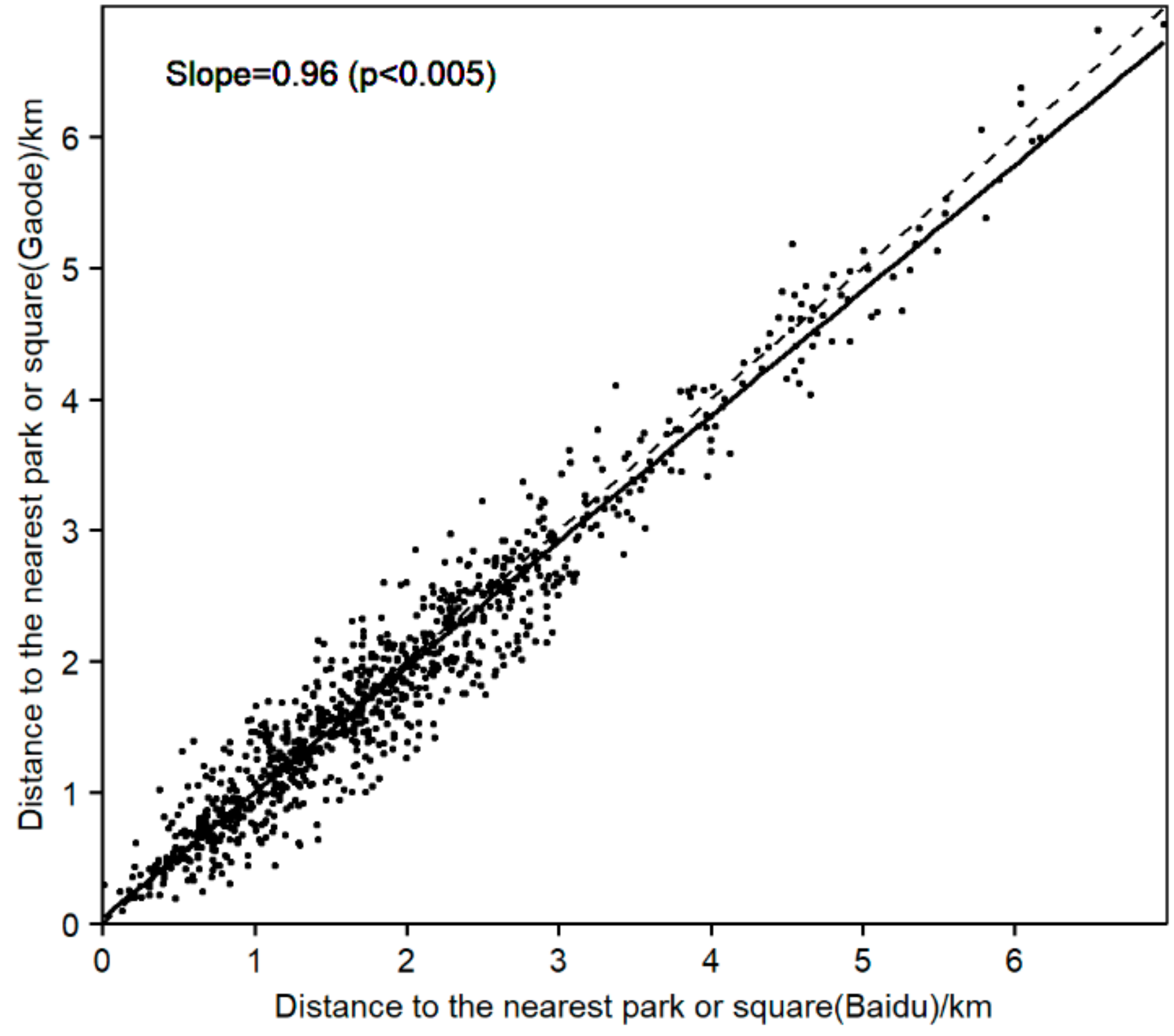
Internet-based geospatial data from open platforms (e.g., Google Maps API, Baidu Map API, Gaode Map API) play a more important role in understanding cities [24]. Here we mainly used the Baidu Map API to retrieve the distance or location information for indices. The advantage was that the travel distance from the Baidu Map API was more accurate to measure accessibility than the Euclidean distance and travel time. The Euclidean distance often could not represent the real origin-destination distance, while the travel time depended heavily on traffic status when taking a trip. However, data from commercial companies might be biased and their quality might not be well controlled, which is likely to undermine the soundness of evaluation results. To validate the data retrieved from the Baidu Map API, we compared them with those derived from Gaode Map API, another popular open platform run by private company (Figure 3). For example, the walking distances from both platforms were highly consistent with each other as indicated by the high correlation coefficient of 0.97 and the regression slope of 0.96. To calculate the travel distance from each community to facilities, we first used the location search service API provided by Baidu Map to retrieve the POIs of different destination categories including parks, hospitals, schools (primary and junior high schools), shopping malls, public transport stops, stations (bus stations, railway stations, and airports), and administrative centers. Then, based on the route calculation service API, we calculated the travel distance from each community to the nearest destination of a given facility category. Walking distance was used to represent the accessibility to the nearest parks and public transport stop, while driving distance was applied for other categories of facilities. The computer program we have developed to retrieve travel distance could be available from GitHub (https://github.com/likai-hub/livability-assessment). To calculate the number of restaurants and shops (including convenience stores and supermarkets) within the buffer zone of 0.5 km for each community, we used the location search service API to retrieve the POIs of restaurants and shops. Then, we generated a buffer zone of 0.5 km for each community, and summarized the number of restaurants or shops falling within the zone.
To derive the traffic congestion probability for each community, we first generated a fishnet with 1 km × 1 km grid size, which covered the whole study area, and extracted the coordinates for four corners of each grid. Then, we used the real-time traffic query service API to retrieve the traffic status of each grid during rush hours (6:00 a.m.–9:00 a.m.; 4:00 p.m.–7:00 p.m.). Traffic status information of each grid can be gained every 10 min, including five states: smooth, relatively smooth, slow moving, slight congestion, congestion, and severe congestion. We developed a computer program to automatically extract the daily traffic information, and calculated the probability of traffic congestion as the percentage of the times of retrievals when the traffic status was slight congestion, congestion, and severe congestion to the total times of retrievals. The code is available from GitHub (https://github.com/likai-hub/livability-assessment). Finally, the probability for each community was estimated using the area-weighted sum method as shown in Equation (2).
Population density directly influenced living environment, because a crowd community could cause noise pollution, and physical and psychological discomfort. We used the location-based big data released by Tencent, a Chinese technology company, which provided services of social network, online games, web portals, etc to ~85% of the population in China (https://heat.qq.com/). The users’ login positions on all Tencent platforms, such as QQ and Wechat, were collected in real time, and the total login count could be retrieved at a high spatial resolution (~1 km) through an https-based data interface. We developed a computer program to automatically acquire the total login counts for all locations (points with an interval of 1 km) every 5 min between 21:30 and 22:00 from 4–8 March 2019. The code is available from GitHub (https://github.com/likai-hub/livability-assessment). Then, the fishnet with a size of 1 km was generated and centered at all locations, and the population density for each cell of the fishnet was calculated as the sum of login counts at all times of retrievals.
Annual PM2.5 concentrations of each community were derived from the Global Annual PM2.5 Grids from MODIS, MISR and SeaWiFS Aerosol Optical Depth (AOD) with GWR, which had been successfully used in health and environmental research [49]. This dataset was available at a 1-km spatial resolution from the NASA Socioeconomic Data and Application Center (NASA SEDAC: https://sedac.ciesin.columbia.edu/data/set/sdei-global-annual-gwr-pm2-5-modis-misr-seawifs-aod). We used the average value of annual PM2.5 concentrations from 2014 to 2016 to represent the index of annual PM2.5 concentrations, and derived the index value for each community based on the area-weighted sum method.
We calculated the building density for each community, which was defined as the total building floor area divided by the community area. The outlines of building floor area within each community were digitalized based on the high-resolution Google Earth imagery.

2.3.4. Determining the Weights of Indices

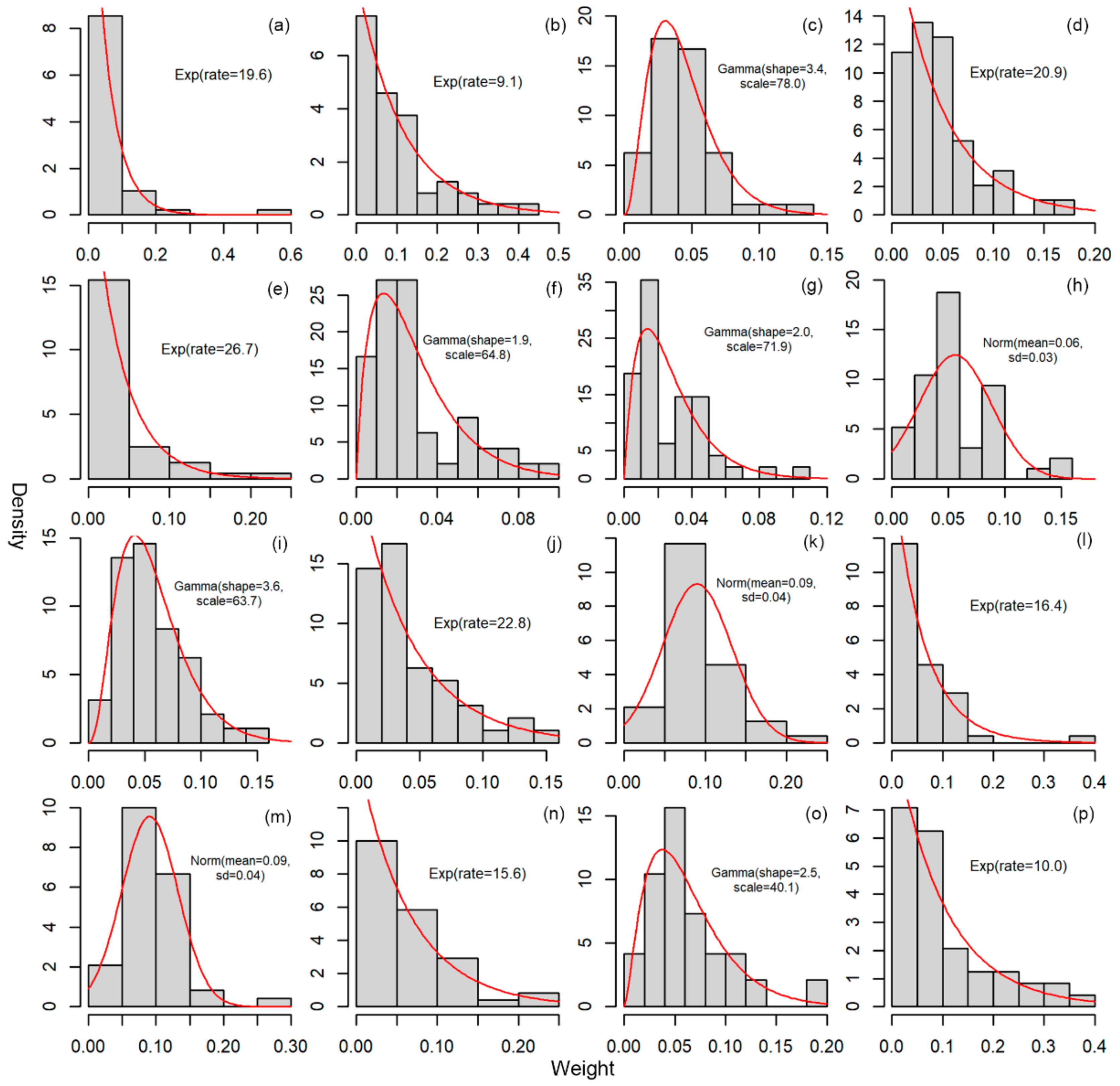
To comprehensively represent the perceptions of the majority to index importance, we applied a combined questionnaire survey and an AHP method to determine the weight of each dimension and index. AHP was one of a multi-criteria decision making method which derived ratio scales from paired comparisons [10,50,51]. The input could be obtained from a subjective opinion such as satisfaction feelings and preference. The advantage of AHP was that it allowed some inconsistency in human judgement among all paired comparisons. To satisfy the input requirements of AHP, we designed a questionnaire to compare the indices two by two, and judged how important they were to the corresponding dimension at their upper level. Seven scales were used to measure the importance between two indices: absolutely more important, much more important, somewhat more important, equally important, somewhat less important, much less important, and absolutely less important. For example, the question to compare the importance of duration of thermal comfort and air pollution was described as: How do you judge that air pollution is compared to the days of thermal comfort regarding their contribution to influence community comfort? (A-Absolutely more important, B-Much important, C-Somewhat more important, D-Equally important, E-Somewhat less important, F-Much less important, G-Absolutely less important). For the five dimensions at the top level and the 16 indices at the bottom level, 33 questions in total were required to make complete comparisons. We made 298 effective questionnaire surveys for 60 randomly selected communities, and converted each into a comparison matrix. AHP was applied to each matrix and got a series of weights to reflect the opinions of one interviewee. The computer program which aimed to run AHP analysis for each questionnaire survey could be downloaded from GitHub (https://github.com/likai-hub/livability-assessment). We analyzed all the weights of a given index from all interviewees, and well fit their distributions using three types of probability distribution functions including exponential, normal, and gamma distribution function (Figure 4). The exponential probability density function (Exp) can be expressed as:
f ( x ) = λ e λ x ,
where λ represents the rate. The normal probability density function (Norm) can be written as:
f ( x ) = 1 2 π σ 2 e 1 2 ( x μ σ ) 2 ,
where μ is the mean, and σ represents the standard deviation (sd). The gamma probability density function (Gamma) can be written as:
f ( x ; k , θ ) = x k 1 e x θ θ k Γ ( k ) ,
where k is shape parameter, θ is scale parameter, and Γ is the gamma function.

2.3.5. Calculating and Classifying Livability Scores

To transform the values of all indices to a comparable scale for aggregation, we used the feature scaling method to rescale data to have values between 0 and 100. For an index whose higher values were more beneficial to livability, the rescaling equation was written as:
X i = V i V m i n V m a x V m i n × 100 ,
where X i and V i were the rescaled and raw values of community i respectively, V m a x and V m i n were the maximum and minimum values among all communities. For the index whose lower values represented better livability, the equation was expressed as:
X i = V m a x V i V m a x V m i n × 100 ,
We aggregated the rescaled values of indices using the weighted sum method to get the scores by dimension and for livability in total. The equation was written as:
S c o r e i = j = 1 N W j × X i j j = 1 N W j ,
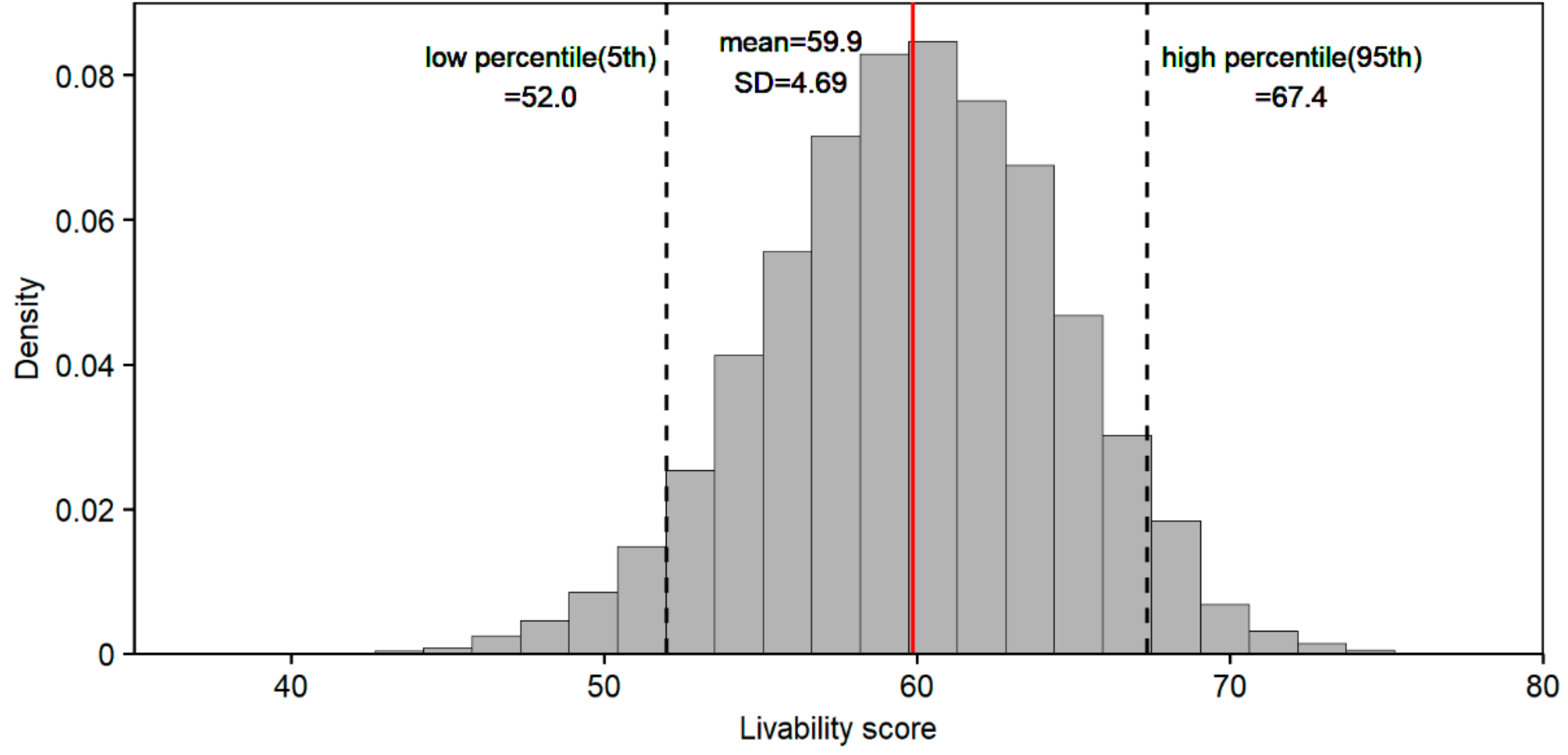
where S c o r e i was the liability score for community i, W j represented the weight for index j, X i j denotes the rescaled value of index j for community i, and N was the total number of indices. For each community, we ran Monte Carlo simulations 10,000 times with a randomly generated weight of each index based on its probability distribution. We used the mean value of 10,000 simulations as the livability score of the community, and calculated the standard deviation to show its uncertainty (Figure 5).
We used the quartile method and set the breaks of intervals at the 90th, 80th, 60th, 40th percentile values to classify livability into 5 classes. The reason we chose this method is that the approximate ranking information can be gained from its class. For example, a community within the first class ranks in the top 10% of overall communities. The five classes included the first class (above 90th percentile), second class (81th–90th percentile), third class (61th–80th percentile), fourth class (41th–60th percentile), and fifth class (below 40th percentile). The higher the class is, the poorer the livability is. When a community lies in the fourth class, measures should be taken to improve some dimensions or indices of livability. A community, which lies at the lower 40th percentile, has overall poor livability, and all-round measures should be adopted to improve the livability. Which aspect(s) should be ameliorated can be identified from the assessment results by dimension or index.

2.3.6. Examining the Relationship between Livability and House Price

Housing price was a sensitive indicator of livability. Ideally, a community with a higher livability score would have higher housing prices. We retrieved the real-estate transaction prices of all communities in June, July, and August of 2019 using a Python-based web page scrawling method from the website of Lianjia, the largest real-estate brokerage company in China (https://linyi.lianjia.com/). The computer program in Python is available from GitHub (https://github.com/likai-hub/livability-assessment). The prices represented the average transaction prices of second-hand houses of communities. We then averaged the prices of these three months, and conducted a regression of housing price against livability score.

3. Results

3.1. Single-Index Assessment

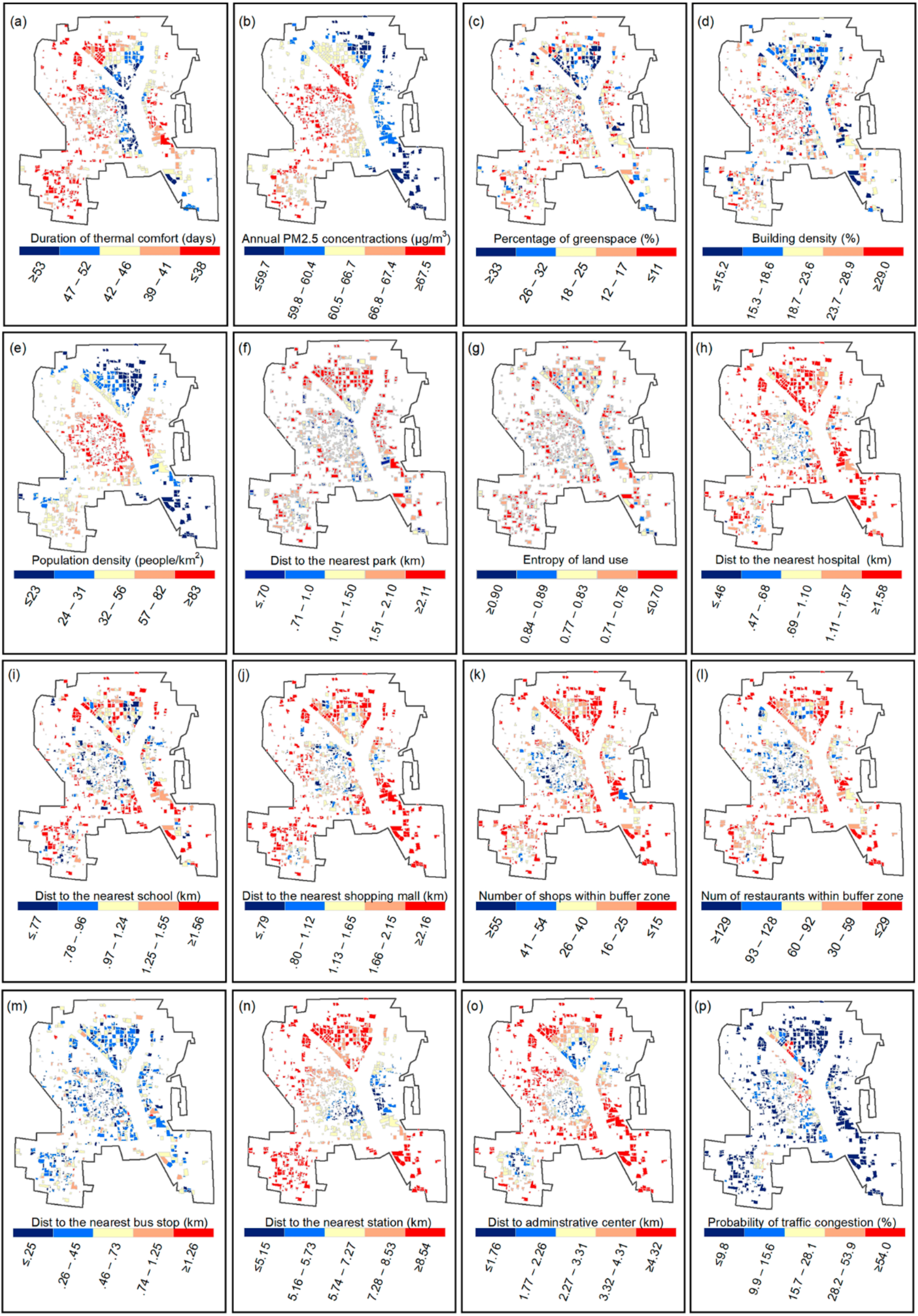
Most indices showed clear patterns across the communities of the study area (Figure 6). There was a clear influence of water bodies on the duration of thermal comfort (Figure 6a), which was characterized by longer duration in the areas close to the Yi River, and shorter in the areas far away from the river. This confirmed previous findings that water bodies had cooling effects on urban temperatures, and mitigated the urban heat island effect [52]. In addition, annual PM2.5 concentrations, which were considered indicators of air quality, were characterized by higher values in the west and lower values in the east (Figure 6b). The relatively poor air quality in the west was mainly due to the densely distributed small-scale factories in industrial zones, which had caused environmental pollution. Although there were industrial zones in the east, air quality was still higher because a large number of high-tech and environment-friendly industries were distributed there.
Communities in the newly developed district at the northern city were characterized by lower building density and population density, higher greenspace coverage but longer distances to public parks, while the communities in the old urban district were the opposite (Figure 6c–g). In the old urban district, communities are often featured by shorter distance to living amenities (e.g., hospital, school, shopping mall), and densely distributed shops and restaurants, due to their longer history of construction, but these amenities were underdeveloped in the newly developed district and industrial zones (Figure 6h–l). Urban residents in the old urban district were convenient to travel due to their proximity to bus, railway stations, and airports (Figure 6m–o). There were some hotspots of traffic congestion which were mainly distributed at the main roads connecting the newly developed and the old urban districts (Figure 6p).

3.2. Assessment by Dimension

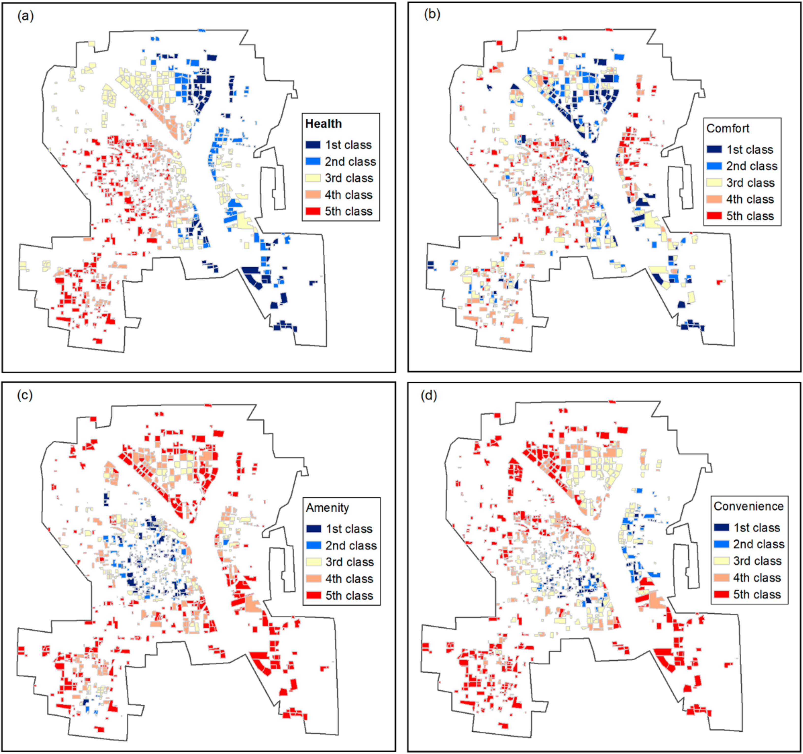
Environmental health manifested itself in a clear spatial pattern, whose conditions deteriorated from the east to the west (Figure 7a). The reason for this was that the industrial zones were mainly distributed in the west and southwest, resulting in environmental pollution and man-made heat emissions from densely distributed small factories. In contrast, better environmental health conditions in the east benefited from sparsely distributed industrial plants and higher percentage of greenspace, which played an important role in reducing particulate matter and mitigating urban heat island effect.
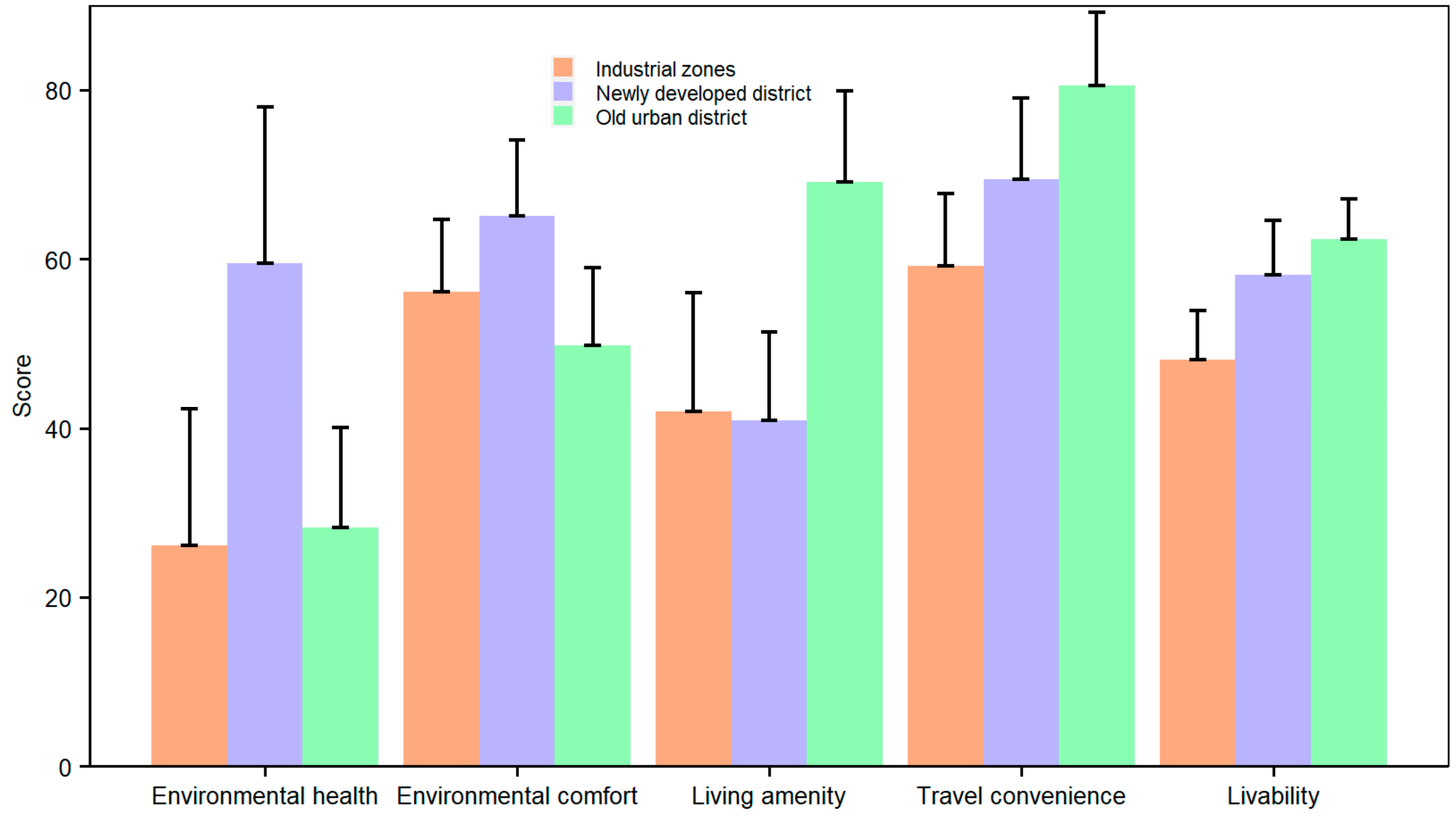
The distinction in environmental comfort between old urban and newly developed districts was clear (Figure 7b). Communities in the newly developed district had the highest level of environmental comfort with a score of 65 due to high greenspace percentage, low building and population density, while the old urban zone had the poorest conditions with a score of 49 (Figure 8). Areas in the southeast also showed higher scores of environmental comfort, which was due to higher greenspace coverage and lower population density. Although these areas were industrial zones, the enterprises here were high-tech and environment-friendly, and thus did not cause severe environmental pollution.
Communities with better conditions of living amenities were mainly in the areas with a longer history of urban development, such as the central old urban district (average score 69) and the administrative center of Hedong and Luozhang District (Figure 7c). The newly developed district had relatively poor living amenity conditions, with an average score of 41 (Figure 8) due to its shorter period of development (thus many of the commercial and institutional facilities like hospitals were still under development) and their less compact urban forms (thus longer distances from communities to the facilities). Industrial zones were also characterized by low scores of living amenities.
Spatial differentiation of travel convenience was evident across the study area (Figure 7d). The old urban district and the administrative center of Hedong District showed the best conditions of travel convenience, with a score as high as 81 (Figure 8), because more public transportation facilities (e.g., bus and railway stations and airports) were distributed within these regions. The conditions of travel convenience were relatively poor in other regions due to longer travel distances to stations and commute centers as well as severe traffic congestion (Figure 8).

3.3. Spatial Pattern of Community Livability

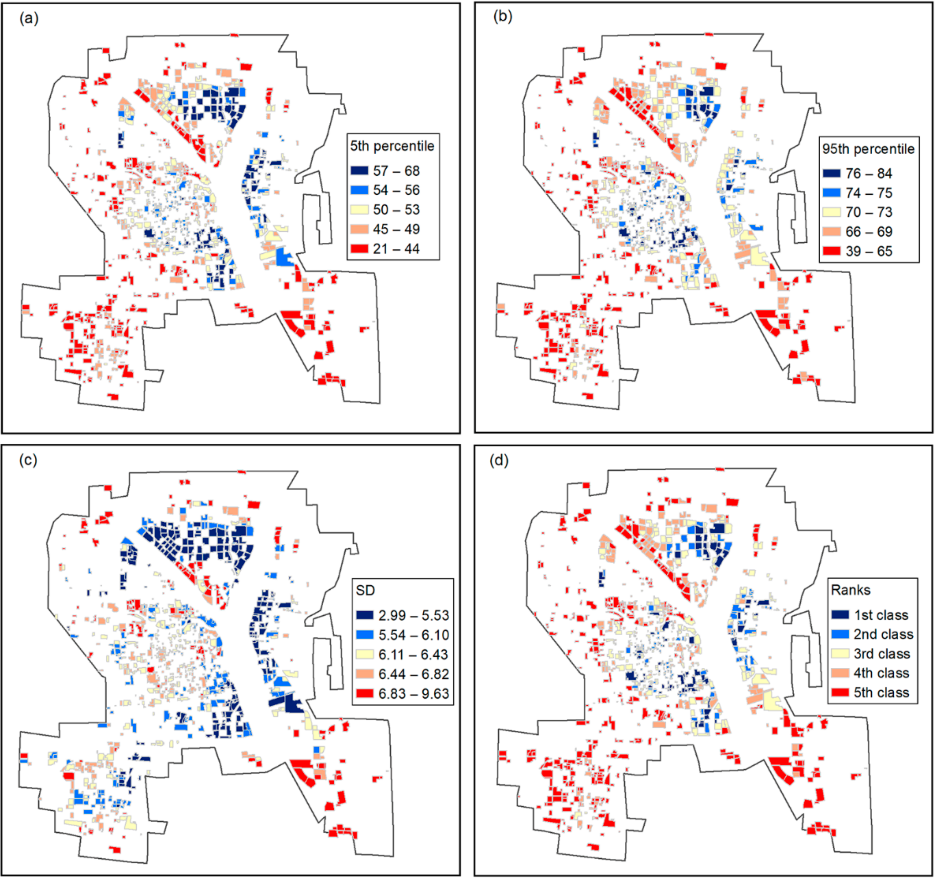
Spatial pattern of community livability was clearly differentiated across the study area (Figure 9d). Spatial patterns of livability scored at the 5th and 95th percentiles were similar to that of mean the livability score (Figure 9a,b). The best livability conditions were observed in the east of the newly developed district, the old urban district, and the center of Hedong district. Although overall livability scores of communities in these regions were higher, they had their own disadvantages for specific dimensions. The east of the newly developed district had better conditions of environmental health and comfort, but poorer conditions of living amenity. These conditions were opposite for the old urban district. The industrial zones in the west, southwest, and southeast of the study area showed the worst livability conditions with the lowest score of 48 (Figure 8). The areas in newly developed district, Hedong district, and the Luozhuang district had relatively lower uncertainties as indicated by the small standard deviations, while the regions in the old urban district and the southeast had higher uncertainties (Figure 9c).
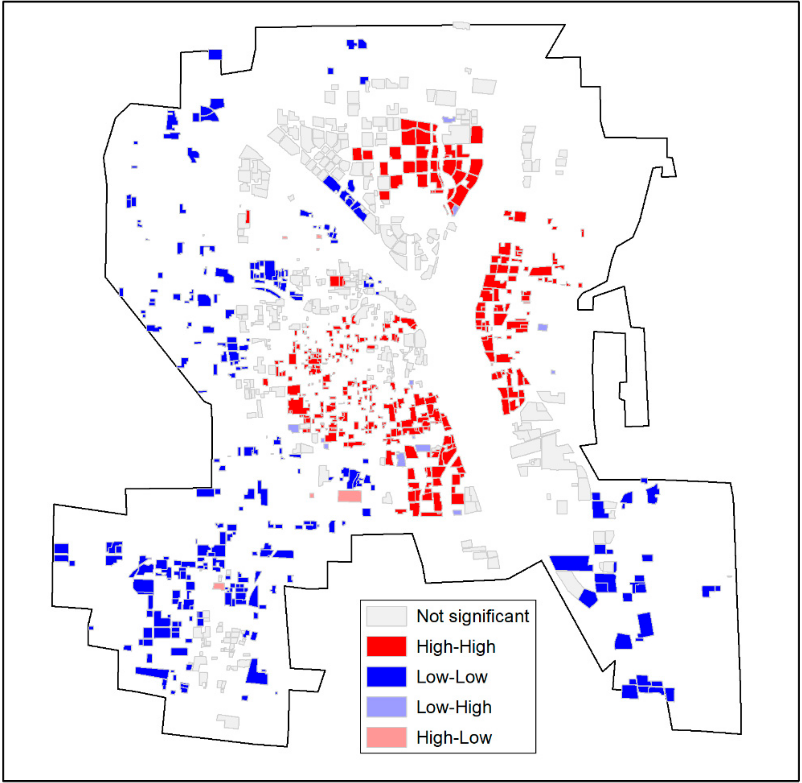
We calculated the Global Moran’s I and the Anselin Local Moran’s I to characterize the spatial patterns of livability scores for all communities. Given the varied distance–decay relationships over the study area, we chose Gaussian kernel function and the adaptive kernel method to create a spatial weight matrix, which allowed us to adjust the bandwidth for each location to ensure equal or near-equal coverage. We calculated these two statistics using the Geoda software downloaded from this link: https://geodacenter.github.io/. The high positive Moran’s statistic of 0.74 (p < 0.01) indicated that livability scores were not randomly distributed among the communities of our study area, and the spatial distribution of the high/low livability scores were more clustered than would be expected. The reason was that factors which influenced the livability of communities were not stochastic, but were determined by location, natural environment, history, and so forth. The Anselin Local Moran’s I statistic results indicated the hotspots and cold spots of livability score clusters (Figure 10). Significant clusters of high scores were found in the east of the newly developed region, the old urban district, and the administrative center of Hedong district. These regions often had a long history of development or were newly constructed with complete infrastructures and favorable environmental conditions. Communities within the industrial zones or on the periphery of the study area demonstrated low score clusters. These regions were often characterized by poor environmental health and comfort, and thus had generally lower livability scores.

3.4. The Relationship between Livability and House Price

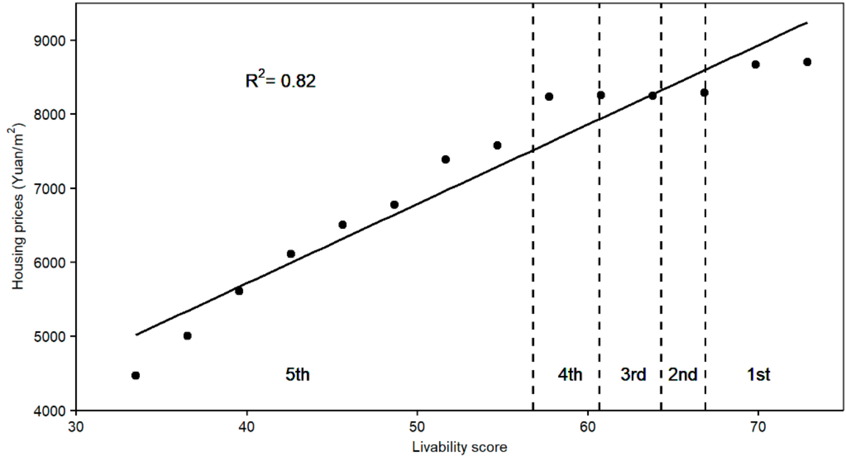
The results showed that the pattern of housing prices was generally consistent with the pattern of our derived livability score (Figure 9 and Figure 11). We found that communities of the first-class livability had the highest housing prices of 8606 CNY/m2 on average, followed by those of the second, third, fourth, and fifth classes, whose housing prices were 8288, 8250, 8230, and 7451 CNY/m2, respectively. Housing prices were significantly correlated with livability scores (R2 = 0.82, p < 0.01) (Figure 12), because high quality of life provided by a livable community is high in demand, which increases market prices. However, the influencing factors of housing prices are complicated, and sometimes one factor might cause a great change in prices, such as school district or location. As a result, an expensive community does not necessarily mean that it is livable, nor that it provides high quality of life. High prices might make residents unable to afford a house that meets their demands, or may cause economic pressure.

4. Discussion

4.1. Model Advantages

Rapid urbanization is causing substantial changes in the urban environment, which influences inhabitants’ livability [3,4]. Understanding the dynamics of livability in time and in great detail is useful to reveal the evolution of urban structure theoretically, and to quickly take measures to address inhabitation problems arising from urbanization [53]. For this purpose, we developed an effective model for spatially explicit community-level livability assessment by combining remote sensing data, big geospatial data, and questionnaire survey data. Our innovative hierarchical livability index system provides a convenient way to organize, understand, and compare the various dimensions/aspects of living conditions among urban communities. Firstly, the hierarchical index system of livability assessment is more flexible compared to a single-tier system [9], and is able to gain information about livability in an organized and detailed way. At the top level, we adopt the widely used dimensions which have been proven to reflect livability comprehensively, while the indices at the bottom level can be modified according to the actual situations of the study area. Secondly, the data for selected indices allows global or national coverage, and are available in a labor-saving way and at no/low costs, which makes our model easy to extend to other areas [16,18]. The extendibility of our model also manifests itself in the selection of a prefecture-level city (i.e., Linyi) as the study area where data availability is less abundant than that in metropolis like Beijing and New York. Thirdly, the data sources for selected indices are regularly updated in a shorter period, so that the assessment results can track the real-time changes in livability. Fourthly, our study showed that all assessment procedures could be streamlined by computer programming, so this is an efficient model with a high scalability. The scripts can be found in GitHub (https://github.com/likai-hub/livability-assessment). Finally, we proposed an innovative approach to calculate the livability score and its uncertainty in each community, which few studies have done before, by including all personal perceptions to the importance of indices from questionnaire surveys and using the Monte Carlo simulation method. To sum up, our model can retrieve the spatial pattern of livability at fine scales (i.e., community level) in an automatic, accurate, and dynamic way, which provides a robust tool for urban planning and governance.

4.2. Understanding the Pattern of Livability

Moreover, the hierarchical structure of the model indexing system is helpful for organizing, understanding, and comparing the underlying influencing factors of livability at different stages of urban development [11,19,54]. Urban land use properties exert a strong influence on environmental health and comfort [17]. For example, industrial zones often have poor conditions of environmental comfort due to high heat emission and severe air pollution. Natural conditions usually strengthen or weaken the effects of land use properties on livability [9,33,34]. For example, the Yi River, which flows through the Linyi city, increases the duration of thermal comfort in areas along the river, and the prevailing southeasterly wind direction during summer causes that temperature mitigation effect at the west riverside to be stronger than that in the east (Figure 6a). The effects of urban development history on livability are notable, as indicated by the distinction between old urban and newly developed districts [11,19]. Urban development stages are closely related to urban forms at different scales, which are comprehensively reflected by a variety of factors including road networks, land use composition and configuration, population density, and so forth [54]. Therefore, development stage and its associated urban forms could reflect the basic local information, and influence livability. The old urban district has a longer history of development, so this region has rich resources of institutional facilities like education and health services, a good transport system, and convenient living amenities (e.g., dense shops). However, longer development history has negative effects on livability, because urban planning and construction at early stages may not meet the higher standard of living environment at present. Therefore, older urban districts often have a high population density, crowded buildings, and a low percentage of greenspace, which is not favorable for living. In contrast, the newly developed district, which has been carefully planned and constructed for a modern urban society with a high density of private cars, was characterized by an excellent greenspace system and a low population density. But the living amenities (e.g., shops) and public transport systems were not well constructed or were sparsely distributed due to its shorter period of development and the sprawling urban form. In addition, marketing factors like land price may influence the development of living amenities such as supermarkets and restaurants [19,41]. For example, high rent could prevent businesses from entering the newly developed district, resulting in a low livability score for living amenities.

4.3. Policy Implications

Our assessments retrieve single-index, dimensional, and overall livability information, which have great implications for urban governance, and gives substantial support for smart city construction. With high spatial and temporal resolution and a hierarchical index structure, our model could help identify the weaknesses of individual communities, so that pertinent measures can be taken to address the problems and to improve its livability. For example, our study in the Linyi city showed that the communities in the old urban district have serious problems in terms of environmental comfort. With regards to urban governance, this region should restrict the immigration of populations, increase greenspace within and without communities, and optimize road networks to make inhabitants’ living environments more comfortable. The communities in the newly developed district have poor conditions of living amenities and travel convenience. It is important for the government to accelerate the infrastructure development and improve institutional facilities like schools, hospitals, and public transportation systems in the new district in the northern city. It is also important to restrict the land price and rent price so that more commercial facilities like supermarkets can move in. Industrial zones have poor conditions for all dimensions of livability. Priority should be given to strictly manage the small factories that cause environmental pollution. Public and commercial service facilities should be improved to promote livability so that urban residents in the industrial zones can live healthily, comfortably, and conveniently.

4.4. Limitations

Though there is no agreement upon the definition of livability, it is clear that livability is more than the properties of living environment (e.g., travel convenience, infrastructures), and the personal feeling or the resident’s desire of a place also influences the degree of livability [14]. Therefore, the assessment of both objective living environments and the subjective satisfaction of residents’ lives matter. In our research, to consider resident perceptions, we follow the human-oriented principle to select the indices which have been proven to exert a substantial influence on residents’ quality of life. Moreover, we collect the judgements of index importance to livability using extensive questionnaire surveys to determine the weights of indices, and input all weight information into the process of livability score calculation. However, much more effort should still be made to figure out the relationship between livability and residents’ satisfaction. This question will become much more complicated when we also have to consider the influence of personal characteristics (i.e., age, gender, job, income) on satisfaction and livability [5,23,55]. Doing such research also requires extensive and detailed questionnaire surveys to collect basic information on residents and their perceptions towards livability. These expansions are beyond the scope of our research, but are worth exploring deeply in future work.

5. Conclusions

We developed a practical and effective model to retrieve the spatial pattern of livability at fine scales in an automatic, accurate, and dynamic way, and provide a robust tool for urban planning and governance. Our application of this model to Linyi city has got reliable assessment results as indicated by the model effectiveness evaluation. The case study in the Linyi city showed that old urban and newly developed districts had relatively high livability, but both regions had their weaknesses—the old district had severe problems in the dimension of environmental comfort, so measures should be taken to control population growth and improve greenspace and road networks; the newly developed district had poor conditions of living amenities and travel convenience, so public and commercial service infrastructure should be improved to make the residents’ life more convenient. Industrial zones have the poorest livability from all dimensions. For the industrial zones, environment-friendly enterprises should be encouraged, while small factories that cause environmental pollution should be shut down or upgraded to be harmless to the environment.
Our developed assessment model driven by remote sensing and Internet-based big geospatial data would be of great interest to governors who need the latest and fine-grained livability information. The advantage is that the data fed into the model are updated on a regular basis, and this model has the potential to be streamlined in order to provide efficient evaluation results for urban governess of a specific city from data acquisition to livability score calculations. Our model would also be of interest to researchers in remote sensing, as it bridges the gap between remote sensing and the theoretical concept of livability, and broadens the applications of remote sensing technology in decision-making processes.

Author Contributions

Conceptualization, L.Z., Y.G., C.Z., J.M. and Y.Z.; Funding acquisition, L.Z. and Y.G.; Methodology, L.Z., Y.G., C.Z., J.M., L.J., Y.Z. and W.T.; Writing—original draft, L.Z., Y.G., C.Z., J.M., L.J., Y.Z. and W.T.; Writing—review and editing, L.Z., Y.G., C.Z., J.M., L.J., Y.Z. and W.T. All authors have read and agreed to the published version of the manuscript.

Funding

This research was funded by the National Natural Science Foundation of China (grant no. 42001373, 41701220 and 41871074), and the Shandong Provincial Natural Science Foundation, China (grant no. ZR2019BD040). Chi Zhang is supported by the Taishan Scholars Program of Shandong, China (grant no. ts201712071). Yuansuo Zhang is supported by the Supporting Plan for Cultivating High Level Teachers in Colleges and Universities in Beijing (grant no. CIT&TCD20180326).

Acknowledgments

We thank Hui Wang, Chunyan Xing, Xi Ren, Chenhao Li, Yufei Du for conducting questionnaire surveys and digitalizing the boundaries of communities. We thank David Frantz for providing the FORCE software to preprocess Sentinel-2 images.

Conflicts of Interest

The authors declare no conflict of interest.

References

  1. Seto, K.C.; Güneralp, B.; Hutyra, L.R. Global forecasts of urban expansion to 2030 and direct impacts on biodiversity and carbon pools. Proc. Natl. Acad. Sci. USA 2012, 109, 16083–16088. [Google Scholar] [CrossRef] [PubMed] [Green Version]
  2. Wu, J. Urban ecology and sustainability: The state-of-the-science and future directions. Landsc. Urban Plan. 2014, 125, 209–221. [Google Scholar] [CrossRef]
  3. Grimm, N.B.; Faeth, S.H.; Golubiewski, N.E.; Redman, C.L.; Wu, J.; Bai, X.; Briggs, J.M. Global Change and the Ecology of Cities. Science 2008, 319, 756–760. [Google Scholar] [CrossRef] [PubMed] [Green Version]
  4. Bai, X.; McPhearson, T.; Cleugh, H.; Nagendra, H.; Tong, X.; Zhu, T.; Zhu, Y.-G. Linking Urbanization and the Environment: Conceptual and Empirical Advances. Annu. Rev. Environ. Resour. 2017, 42, 215–240. [Google Scholar] [CrossRef] [Green Version]
  5. Zhan, D.; Kwan, M.-P.; Zhang, W.; Fan, J.; Yu, J.; Dang, Y. Assessment and determinants of satisfaction with urban livability in China. Cities 2018, 79, 92–101. [Google Scholar] [CrossRef]
  6. Gong, P.; Liang, S.; Carlton, E.J.; Jiang, Q.; Wu, J.; Wang, L.; Remais, J.V. Urbanisation and health in China. Lancet 2012, 379, 843–852. [Google Scholar] [CrossRef]
  7. Gong, P.; Li, X.; Zhang, W. 40-Year (1978–2017) human settlement changes in China reflected by impervious surfaces from satellite remote sensing. Sci. Bull. 2019, 64, 756–763. [Google Scholar] [CrossRef] [Green Version]
  8. Zhou, Y.; Li, X.; Asrar, G.R.; Smith, S.J.; Imhoff, M. A global record of annual urban dynamics (1992–2013) from nighttime lights. Remote. Sens. Environ. 2018, 219, 206–220. [Google Scholar] [CrossRef]
  9. Zhang, W. Index system and method of residential environmental evaluation in inner cities. Sci. Geogr. Sin. 2007, 27, 17–23. [Google Scholar]
  10. Xu, Y.; Sun, J.; Zhang, J.; Xu, Y.; Zhang, M.; Liao, X. Combining AHP with GIS in synthetic evaluation of environmental suitability for living in China’s 35 major cities. Int. J. Geogr. Inf. Sci. 2012, 26, 1603–1623. [Google Scholar] [CrossRef]
  11. Liu, J.; Han, J. Does a Certain Rule Exist in the Long-Term Change of a City’s Livability? Evidence from New York, Tokyo, and Shanghai. Sustainability 2017, 9, 1681. [Google Scholar] [CrossRef] [Green Version]
  12. Onnom, W.; Tripathi, N.K.; Nitivattananon, V.; Ninsawat, S. Development of a Liveable City Index (LCI) Using Multi Criteria Geospatial Modelling for Medium Class Cities in Developing Countries. Sustainability 2018, 10, 520. [Google Scholar] [CrossRef] [Green Version]
  13. Ruth, M.; Franklin, R.S. Livability for all? Conceptual limits and practical implications. Appl. Geogr. 2014, 49, 18–23. [Google Scholar] [CrossRef] [PubMed] [Green Version]
  14. Ahmed, N.O.; El-Halafawy, A.M.; Amin, A.M. A Critical Review of Urban Livability. Eur. J. Sustain. Dev. 2019, 8, 165–182. [Google Scholar] [CrossRef]
  15. Gao, X.; Asami, Y. The External Effects of Local Attributes on Living Environment in Detached Residential Blocks in Tokyo. Urban Stud. 2001, 38, 487–505. [Google Scholar] [CrossRef]
  16. Zhang, Y.; Li, Q.; Wang, H.; Du, X.; Huang, H. Community scale livability evaluation integrating remote sensing, surface observation and geospatial big data. Int. J. Appl. Earth Obs. Geoinf. 2019, 80, 173–186. [Google Scholar] [CrossRef]
  17. Fu, B.; Yu, D.; Zhang, Y. The livable urban landscape: GIS and remote sensing extracted land use assessment for urban livability in Changchun Proper, China. Land Use Policy 2019, 87, 104048. [Google Scholar] [CrossRef]
  18. Zhao, Y.; Zhang, G.; Lin, T.; Liu, X.; Liu, J.; Lin, M.; Ye, H.; Kong, L. Towards Sustainable Urban Communities: A Composite Spatial Accessibility Assessment for Residential Suitability Based on Network Big Data. Sustainability 2018, 10, 4767. [Google Scholar] [CrossRef] [Green Version]
  19. Zhan, D.; Zhang, W.; Yu, J.; Chen, L.; Dang, Y. Spatial characteristics and forming mechanism of urban livability in Beijing based on objective evaluation. Areal Res. Dev. 2016, 35, 68–73. [Google Scholar]
  20. Chen, L.; Zhang, W.; Li, Y. Urban residential suitability evaluation of Dalian’s residents. Acta Geogr. Sin. 2008, 63, 1022–1032. [Google Scholar]
  21. Chen, L.; Zhang, W.; Yang, Y.; Yu, J. Disparities in residential environment and satisfaction among urban residents in Dalian, China. Habitat Int. 2013, 40, 100–108. [Google Scholar] [CrossRef]
  22. Norouzian-Maleki, S.; Bell, S.; Hosseini, S.-B.; Faizi, M. Developing and testing a framework for the assessment of neighbourhood liveability in two contrasting countries: Iran and Estonia. Ecol. Indic. 2015, 48, 263–271. [Google Scholar] [CrossRef] [Green Version]
  23. Ma, J.; Dong, G.; Chen, Y.; Zhang, W. Does satisfactory neighbourhood environment lead to a satisfying life? An investigation of the association between neighbourhood environment and life satisfaction in Beijing. Cities 2018, 74, 229–239. [Google Scholar] [CrossRef]
  24. Liu, X.; Song, Y.; Wu, K.; Wang, J.; Li, D.; Long, Y. Understanding urban China with open data. Cities 2015, 47, 53–61. [Google Scholar] [CrossRef]
  25. Zhou, D.; Xiao, J.; Bonafoni, S.; Berger, C.; Deilami, K.; Zhou, Y.; Frolking, S.; Yao, R.; Qiao, Z.; Sobrino, J.A. Satellite Remote Sensing of Surface Urban Heat Islands: Progress, Challenges, and Perspectives. Remote Sens. 2019, 11, 48. [Google Scholar] [CrossRef] [Green Version]
  26. Zhang, K.; De Leeuw, G.; Yang, Z.; Chen, X.; Su, X.; Jiao, J. Estimating Spatio-Temporal Variations of PM2.5 Concentrations Using VIIRS-Derived AOD in the Guanzhong Basin, China. Remote Sens. 2019, 11, 2679. [Google Scholar] [CrossRef] [Green Version]
  27. Long, Y.; Thill, J.-C. Combining smart card data and household travel survey to analyze jobs–housing relationships in Beijing. Comput. Environ. Urban Syst. 2015, 53, 19–35. [Google Scholar] [CrossRef] [Green Version]
  28. Li, J.; Roy, D. A Global Analysis of Sentinel-2A, Sentinel-2B and Landsat-8 Data Revisit Intervals and Implications for Terrestrial Monitoring. Remote Sens. 2017, 9, 902. [Google Scholar] [CrossRef] [Green Version]
  29. Wan, Z. New refinements and validation of the MODIS Land-Surface Temperature/Emissivity products. Remote Sens. Environ. 2008, 112, 59–74. [Google Scholar] [CrossRef]
  30. Higasa, T. Urban Planning; Kiotitz Corporation Press: Tokyo, Japan, 1977. [Google Scholar]
  31. Asami, Y. Residential Environment: Methods and Theory for Evaluation; University of Tokyo Press: Tokyo, Japan, 2001. [Google Scholar]
  32. Dang, X.; Yu, J.; Zhang, W.; Chen, L.; Zhan, D. Study on evaluation of livable Beijing based on subjective feelings. Hum. Geogr. 2015, 30, 59–65. [Google Scholar]
  33. Saitluanga, B.L. Spatial Pattern of Urban Livability in Himalayan Region: A Case of Aizawl City, India. Soc. Indic. Res. 2014, 117, 541–559. [Google Scholar] [CrossRef]
  34. Węziak-Białowolska, D. Quality of life in cities—Empirical evidence in comparative European perspective. Cities 2016, 58, 87–96. [Google Scholar] [CrossRef]
  35. Mahmoudi, M.; Ahmad, F.; Abbasi, B. Livable streets: The effects of physical problems on the quality and livability of Kuala Lumpur streets. Cities 2015, 43, 104–114. [Google Scholar] [CrossRef]
  36. Dong, H.; Qin, B. Exploring the link between neighborhood environment and mental wellbeing: A case study in Beijing, China. Landsc. Urban Plan. 2017, 164, 71–80. [Google Scholar] [CrossRef]
  37. Brown, B.B.; Yamada, I.; Smith, K.R.; Zick, C.D.; Kowaleski-Jones, L.; Fan, J.X. Mixed land use and walkability: Variations in land use measures and relationships with BMI, overweight, and obesity. Health Place 2009, 15, 1130–1141. [Google Scholar] [CrossRef] [PubMed] [Green Version]
  38. Shamsuddin, S.; Abu Hassan, N.R.; Bilyamin, S.F.I. Walkable Environment in Increasing the Liveability of a City. Procedia Soc. Behav. Sci. 2012, 50, 167–178. [Google Scholar] [CrossRef] [Green Version]
  39. Lund, H. Testing the Claims of New Urbanism: Local Access, Pedestrian Travel, and Neighboring Behaviors. J. Am. Plan. Assoc. 2003, 69, 414–429. [Google Scholar] [CrossRef]
  40. Stanislav, A.; Chin, J.T. Evaluating livability and perceived values of sustainable neighborhood design: New Urbanism and original urban suburbs. Sustain. Cities Soc. 2019, 47, 101517. [Google Scholar] [CrossRef]
  41. Zhang, W. An analysis of the factors that influence the urban residential location selection. Prog. Geogr. 2001, 20, 268–275. [Google Scholar]
  42. Feltynowski, M.; Kronenberg, J.; Bergier, T.; Kabisch, N.; Łaszkiewicz, E.; Strohbach, M.W. Challenges of urban green space management in the face of using inadequate data. Urban For. Urban Green. 2018, 31, 56–66. [Google Scholar] [CrossRef]
  43. Frantz, D.; Roder, A.; Stellmes, M.; Hill, J. An Operational Radiometric Landsat Preprocessing Framework for Large-Area Time Series Applications. IEEE Trans. Geosci. Remote Sens. 2016, 54, 3928–3943. [Google Scholar] [CrossRef]
  44. Frantz, D.; Stellmes, M.; Röder, A.; Udelhoven, T.; Mader, S.; Hill, J. Improving the Spatial Resolution of Land Surface Phenology by Fusing Medium- and Coarse-Resolution Inputs. IEEE Trans. Geosci. Remote Sens. 2016, 54, 4153–4164. [Google Scholar] [CrossRef]
  45. Frantz, D.; Röder, A.; Stellmes, M.; Hill, J. Phenology-adaptive pixel-based compositing using optical earth observation imagery. Remote Sens. Environ. 2017, 190, 331–347. [Google Scholar] [CrossRef] [Green Version]
  46. Pan, T.; Lu, D.; Zhang, C.; Chen, X.; Shao, H.; Kuang, W.; Chi, W.; Liu, Z.; Du, G.; Cao, L. Urban Land-Cover Dynamics in Arid China Based on High-Resolution Urban Land Mapping Products. Remote Sens. 2017, 9, 730. [Google Scholar] [CrossRef] [Green Version]
  47. Li, X.; Zhou, Y.; Asrar, G.R.; Zhu, Z. Creating a seamless 1 km resolution daily land surface temperature dataset for urban and surrounding areas in the conterminous United States. Remote Sens. Environ. 2018, 206, 84–97. [Google Scholar] [CrossRef]
  48. Zhu, W.; Lu, A.; Jia, S. Estimation of daily maximum and minimum air temperature using MODIS land surface temperature products. Remote Sens. Environ. 2013, 130, 62–73. [Google Scholar] [CrossRef]
  49. Van Donkelaar, A.; Martin, R.V.; Brauer, M.; Hsu, N.C.; Kahn, R.A.; Levy, R.; Lyapustin, A.; Sayer, A.M.; Winker, D. Global Estimates of Fine Particulate Matter using a Combined Geophysical-Statistical Method with Information from Satellites, Models, and Monitors. Environ. Sci. Technol. 2016, 50, 3762–3772. [Google Scholar] [CrossRef]
  50. Antognelli, S.; Vizzari, M. Landscape liveability spatial assessment integrating ecosystem and urban services with their perceived importance by stakeholders. Ecol. Indic. 2017, 72, 703–725. [Google Scholar] [CrossRef]
  51. Reis, I.F.; Ferreira, F.A.; Meidutė-Kavaliauskienė, I.; Govindan, K.; Fang, W.; Falcão, P.F. An evaluation thermometer for assessing city sustainability and livability. Sustain. Cities Soc. 2019, 47, 101449. [Google Scholar] [CrossRef]
  52. Deilami, K.; Kamruzzaman, L.; Liu, Y. Urban heat island effect: A systematic review of spatio-temporal factors, data, methods, and mitigation measures. Int. J. Appl. Earth Obs. Geoinf. 2018, 67, 30–42. [Google Scholar] [CrossRef]
  53. Dhingra, M.; Singh, M.K.; Chattopadhyay, S. Rapid Assessment Tool for traditional Indian Neighbourhoods: A Case Study of Alwar Walled City in Rajasthan. Sustain. Cities Soc. 2016, 26, 364–382. [Google Scholar] [CrossRef]
  54. Song, Y.; Long, Y.; Wu, P.; Wang, X. Are all cities with similar urban form or not? Redefining cities with ubiquitous points of interest and evaluating them with indicators at city and block levels in China. Int. J. Geogr. Inf. Sci. 2018, 32, 2447–2476. [Google Scholar] [CrossRef]
  55. Ng, S.L.; Zhang, Y.; Ng, K.H.; Wong, H.; Lee, J.W.Y. Living environment and quality of life in Hong Kong. Asian Geogr. 2018, 35, 35–51. [Google Scholar] [CrossRef]
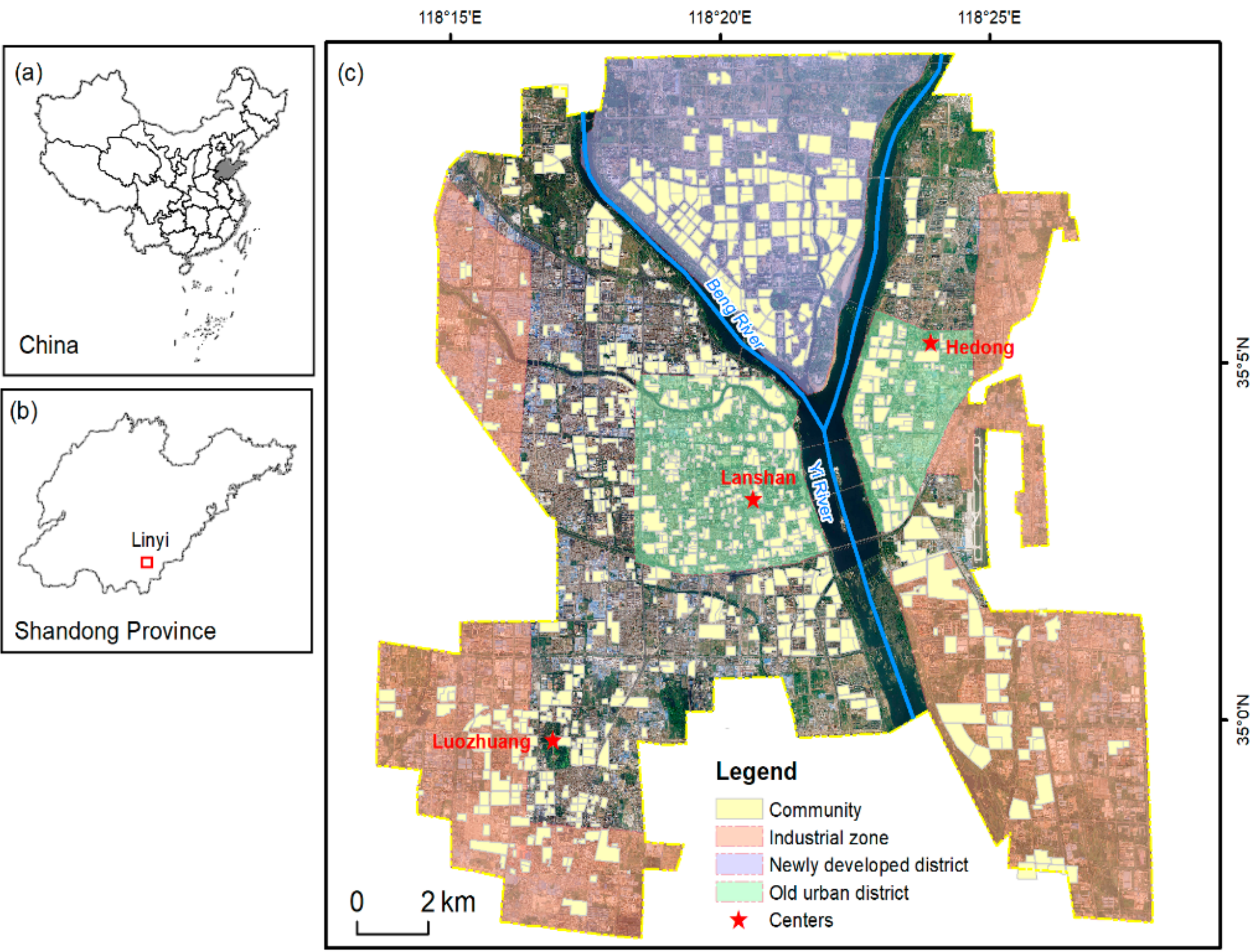
Figure 1. Geographical features of the study area. The inset maps show the geographic location of Linyi (a) in China and (b) in Shandong Province. (c) The main map demonstrates the spatial distribution of communities and urban functional zones. Unlike countries such as the United States and Canada, the community in China often takes the form of a gated residential area with a clear boundary, and consists of several blocks of buildings.
Remotesensing 12 04026 g001
Figure 2. Procedures to develop the livability assessment model. The four steps are shown in the boxes with the bold frame.
Remotesensing 12 04026 g002
Figure 3. Comparison of the walking distance to the nearest park from Baidu Map API and Gaode Map API.
Remotesensing 12 04026 g003
Figure 4. The density and fitted probability distribution of all AHP-derived weights based on a questionnaire survey by index. (ap) represent different indices at the bottom level as shown in Table 1.
Remotesensing 12 04026 g004
Figure 5. The distribution of livability scores for one community derived from Monte Carlo simulations for 10,000 times.
Remotesensing 12 04026 g005
Figure 6. Single–index assessment of livability based on the 16 indices under 4 dimensions, as shown in Table 1. (a,b) spatial patterns of index values within the dimension of environmental health; (cg) spatial patterns of index value within the dimension of environmental comfort; (hl) spatial patterns of index values within the dimension of living amenity; (mp) spatial patterns of index values within the dimension of travel convenience.
Remotesensing 12 04026 g006
Figure 7. Livability assessment by dimension. (a) Environmental health; (b) Environmental comfort; (c) Living amenity; (d) Travel convenience. The communities of the first class were the ones whose scores were above 90th percentile, the second-class communities were the ones whose scores were within the range of the 81st and the 90th percentile, the third-class communities were the ones whose scores were within the range of the 61st and the 80th percentile, the fourth-class communities were the ones whose scores were within the range of the 41st and the 60th percentile, and the fifth-class communities were the ones whose scores were below the 40th percentile.
Remotesensing 12 04026 g007
Figure 8. Average scores of different livability dimensions summarized by urban functional types and overall livability scores summarized by urban functional types.
Remotesensing 12 04026 g008
Figure 9. Spatial patterns of livability scores and its uncertainty for all communities. (a) The 5th percentile of livability scores from Monte Carlo simulations. (b) The 95th percentile of livability scores from Monte Carlo simulations. (c) The standard deviation of livability scores from Monte Carlo simulations. (d) Five livability ranks classified using the quantile method. The communities of the first class were the ones whose scores were above 90th percentile, the second-class communities were the ones whose scores were within the range from 81th to 90th percentile, the third-class communities were the ones whose scores were within the range from 61th to 80th percentile, the fourth-class communities were the ones whose scores were within the range from 41th to 60th percentile, and the fifth-class communities were the ones whose scores were below 40th percentile.
Remotesensing 12 04026 g009
Figure 10. Spatial pattern of clusters of high and low livability scores. Clusters indicate that a high (low) livability score is surrounded primarily by high (low) values.
Remotesensing 12 04026 g010
Figure 11. Spatial pattern of average real-estate transaction prices of communities in 2019.
Remotesensing 12 04026 g011
Figure 12. Relationship between housing prices and livability scores. Housing prices show a significantly positive correlation with livability scores (p < 0.05).
Remotesensing 12 04026 g012
Table 1. A hierarchical index system for livability assessment which includes 4 dimensions at the top level and 16 indices at the bottom level. The positive sign indicates that the higher value of the index is more favorable to livability, and vice versa.
DimensionsIndicesSource
Environmental health (a) Annual PM2.5 concentration (−)NASA SEDAC Global annual PM2.5 product
(b) Duration of thermal comfort (+)MODIS LST products
Environmental comfort (c) Percentage of greenspace (+)Sentinel-2 imagery
(d) Building density (−)Google Earth images
(e) Population density (−)Tencent Location API
(f) Walking distance to the nearest park (−)Baidu Map API
(g) Entropy of land use (+)Sentinel-2 images
Living amenity (h) Driving distance to the nearest hospital (−)Baidu Map API
(i) Driving distance to the nearest school (−)Baidu Map API
(j) Driving distance to the nearest shopping mall (−)Baidu Map API
(k) Number of shops within 0.5-km buffer zone (+)Baidu POIs
(l) Number of restaurants within 0.5-km buffer zone (+)Baidu POIs
Travel convenience (m) Walking distance to the nearest bus stop (−)Baidu Map API
(n) Driving distance to the nearest bus, railway, and airway stations (−)Baidu Map API
(o) Driving distance to the administrative center (−)Baidu Map API
(p) Probability of traffic congestion (−)Baidu Map API
Publisher’s Note: MDPI stays neutral with regard to jurisdictional claims in published maps and institutional affiliations.