
Assessing the Long-Term Evolution of Abandoned Salinized Farmland via Temporal Remote Sensing Data


Abstract
:
1. Introduction
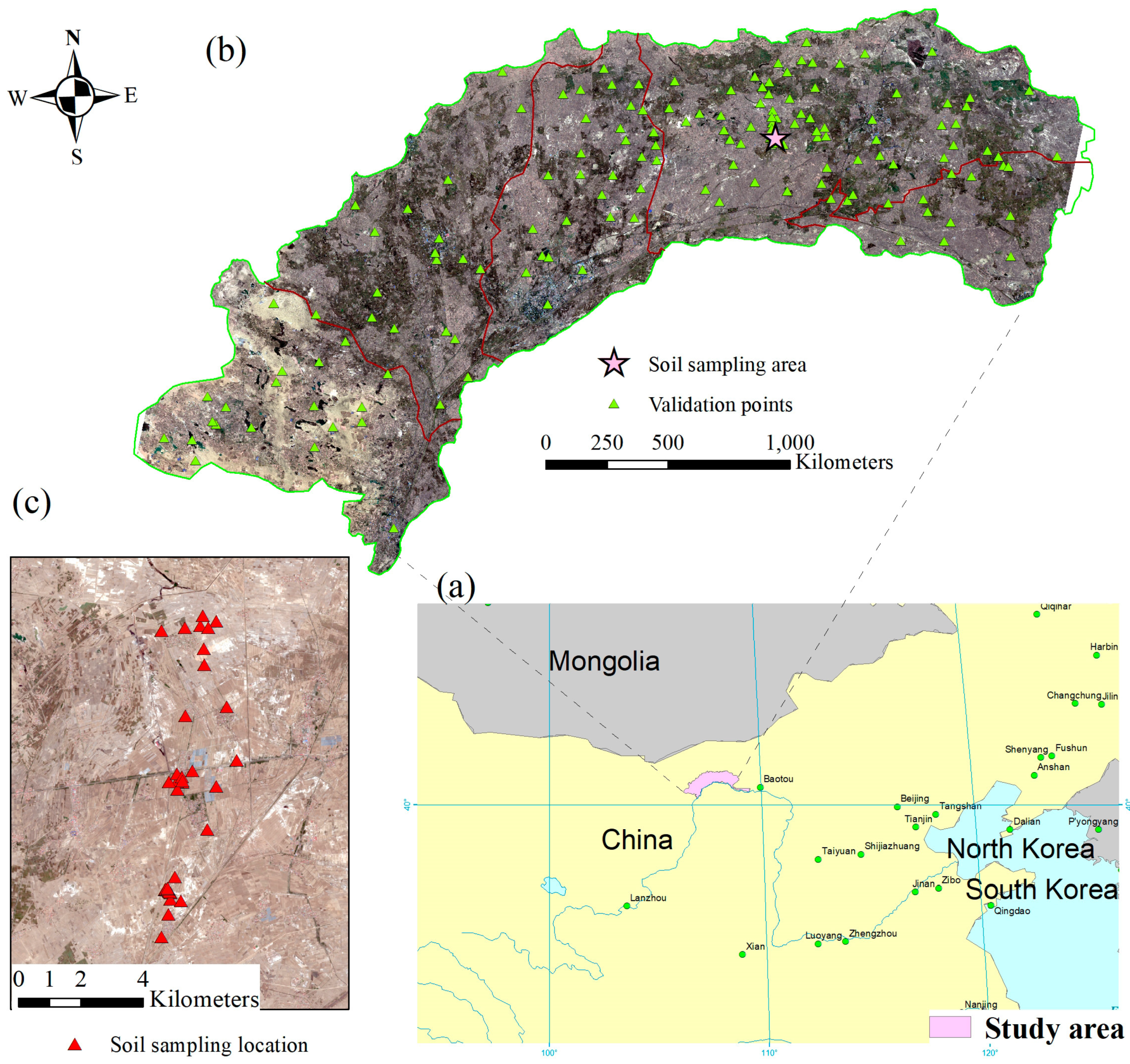
2. Study Area
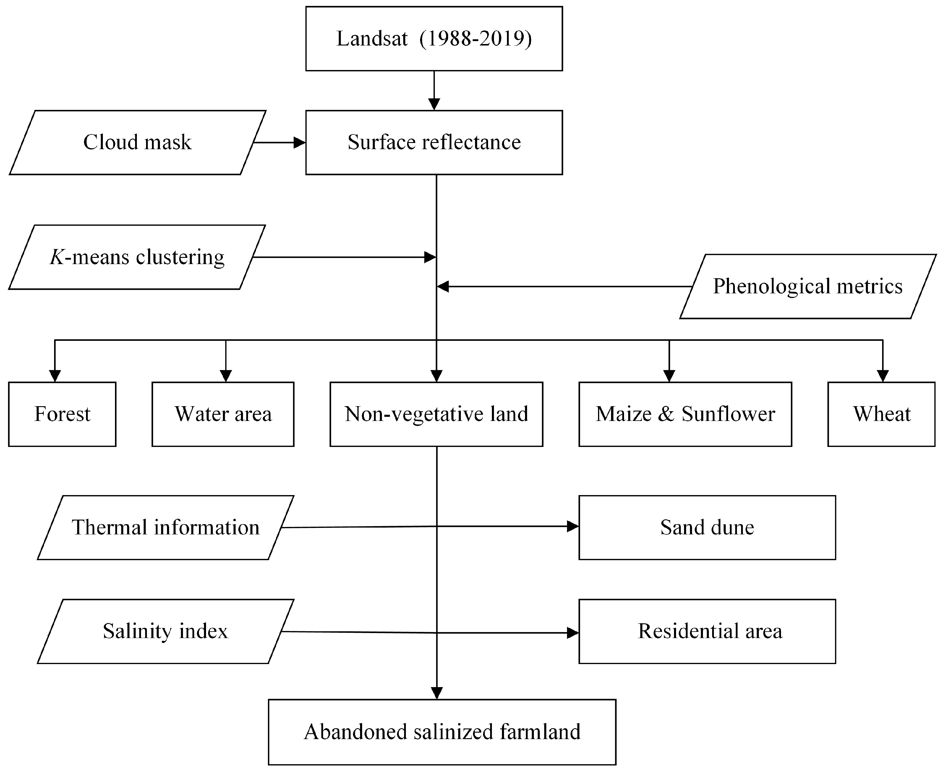
3. Methods
3.1. Data Processing
3.1.1. Satellite Data
3.1.2. Ground Data
3.2. Analyzing Temporal Remotely Sensed Imageries
3.2.1. Land Cover Classification via K-Means Clustering
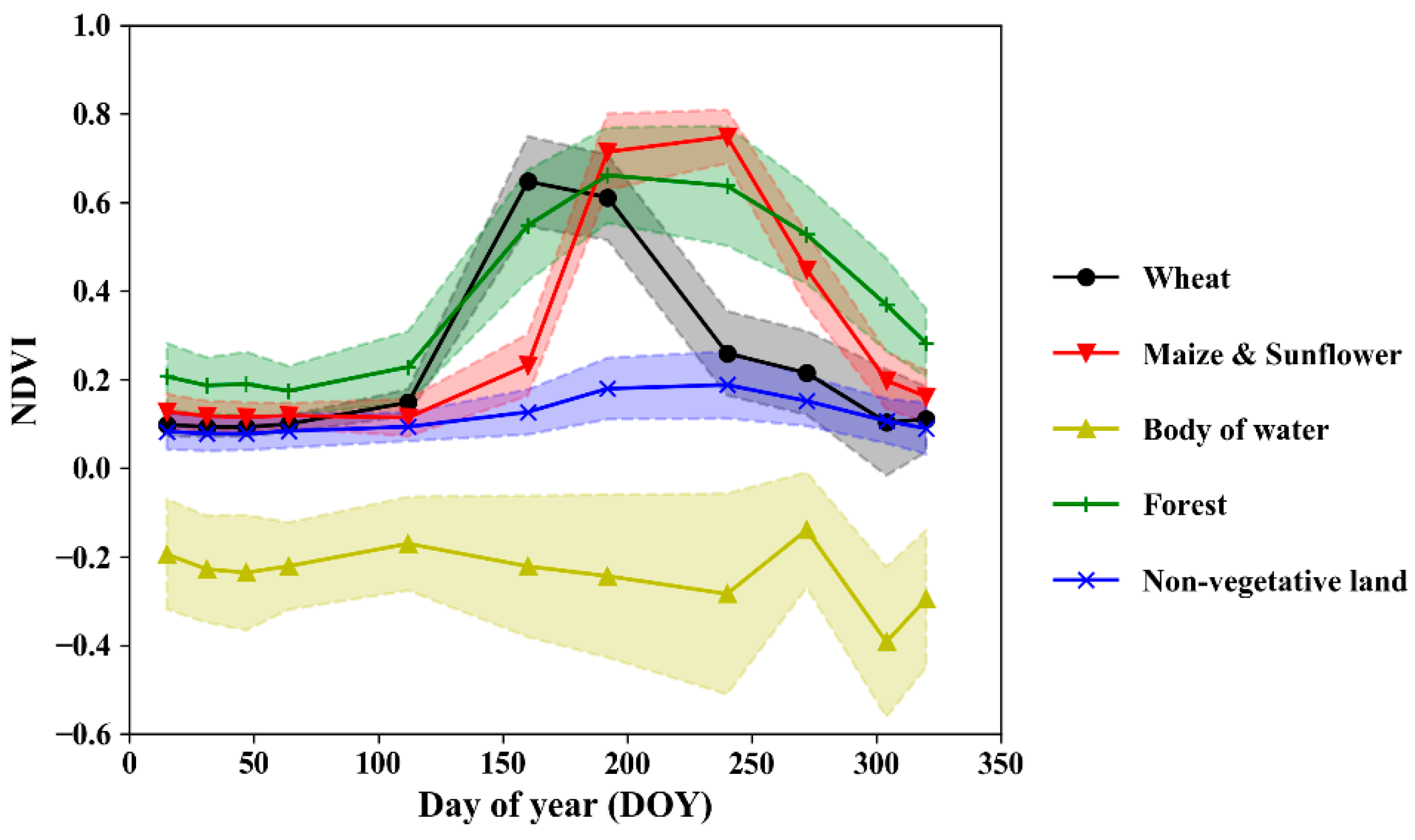
3.2.2. Detecting Cropping Structure Based on Phenological Metrics
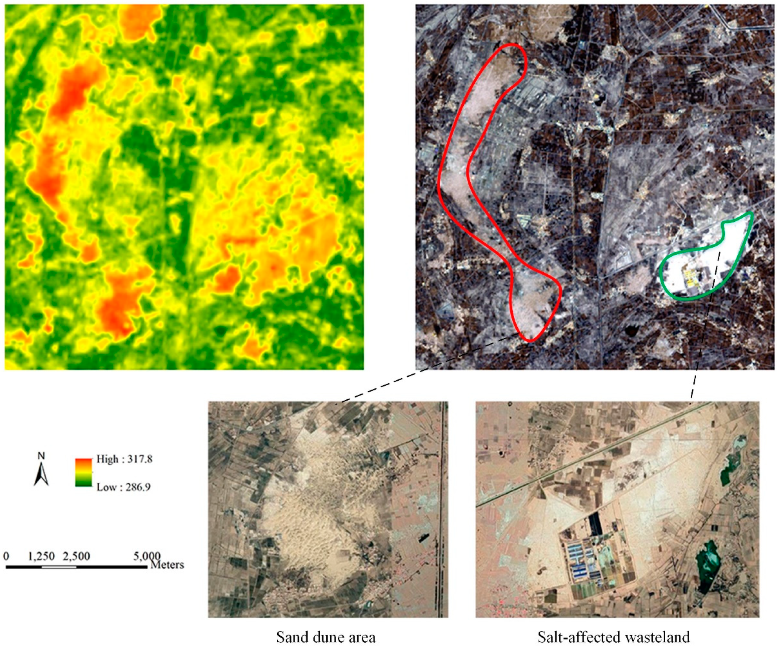
3.3. Detecting Sand Dunes and Deserts Using Thermal Information
3.4. Detecting Abandoned Salinized Farmland
3.5. Performance Measures
4. Results
4.1. Evolution of Cropping Structure in Hetao
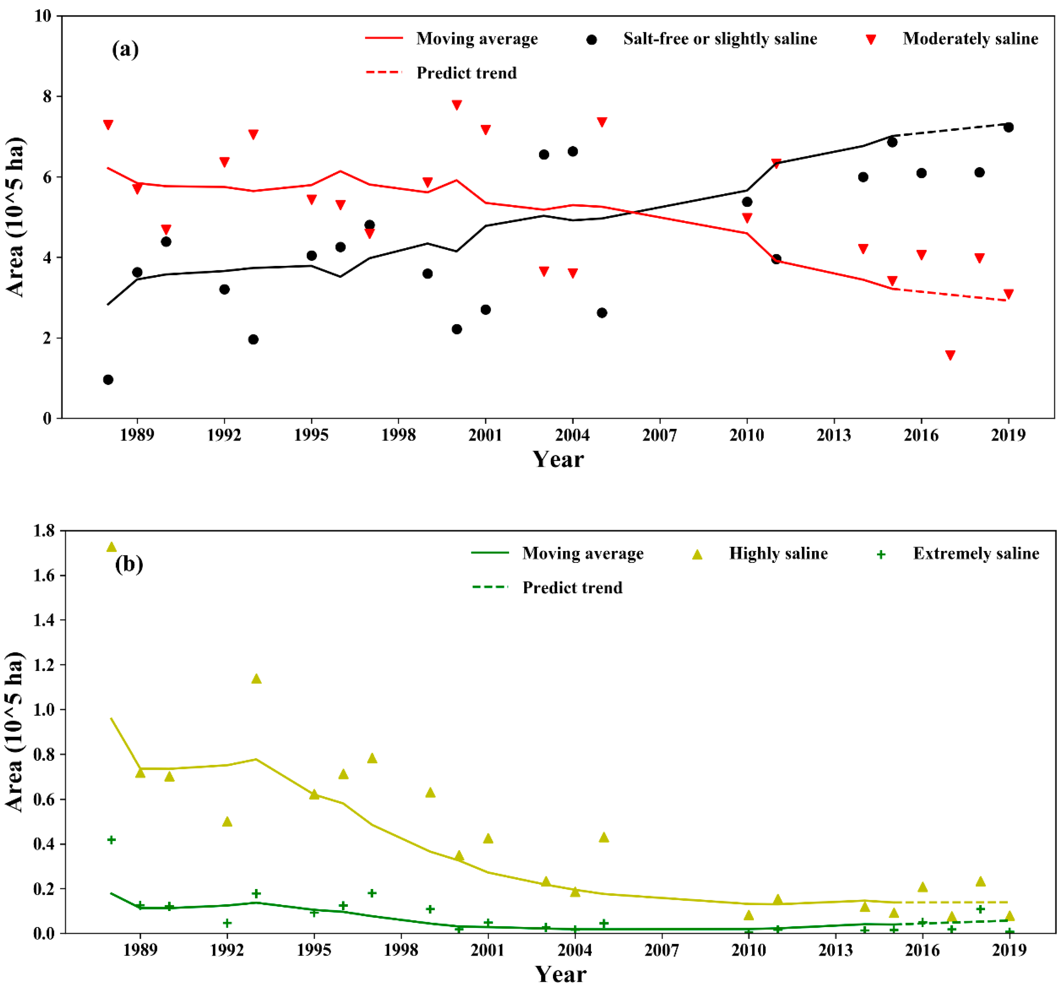
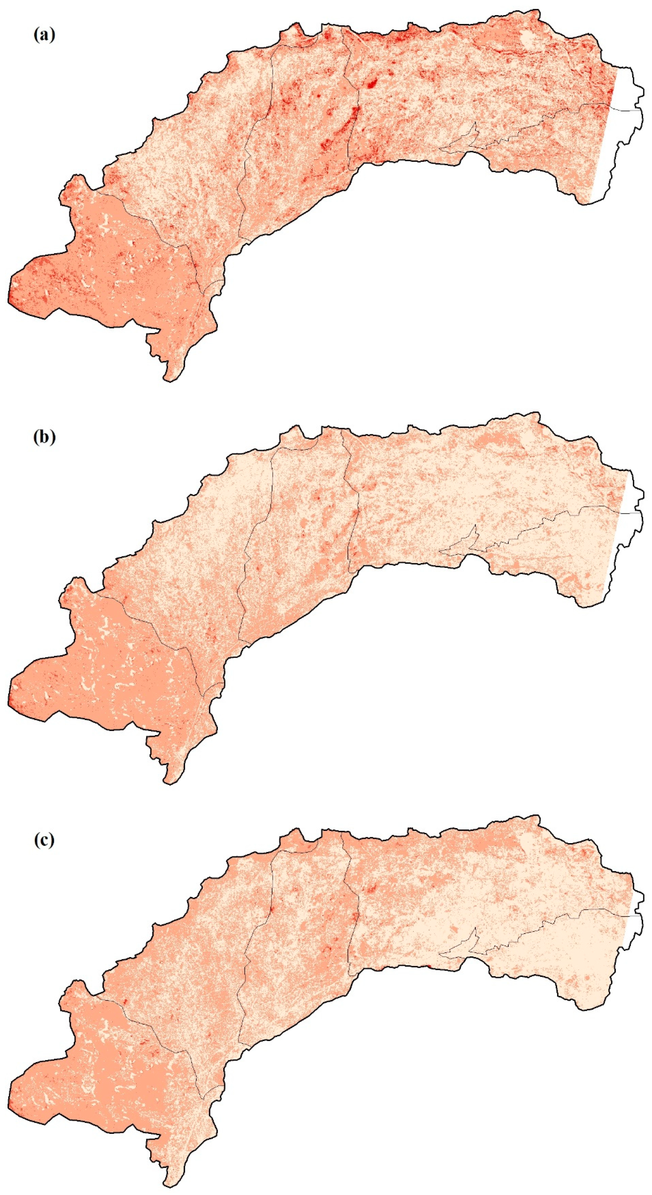
4.2. Desalinization Progress in Hetao
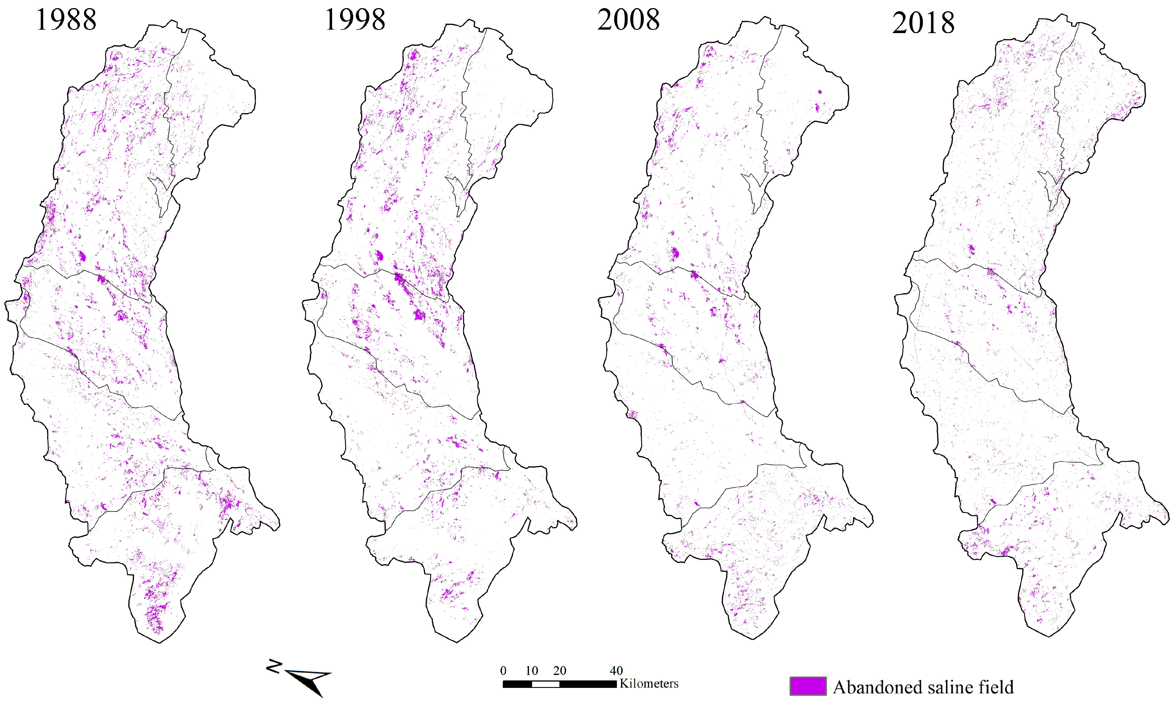
4.3. Spatio-Temporal Pattern of Abandoned Salinized Farmland
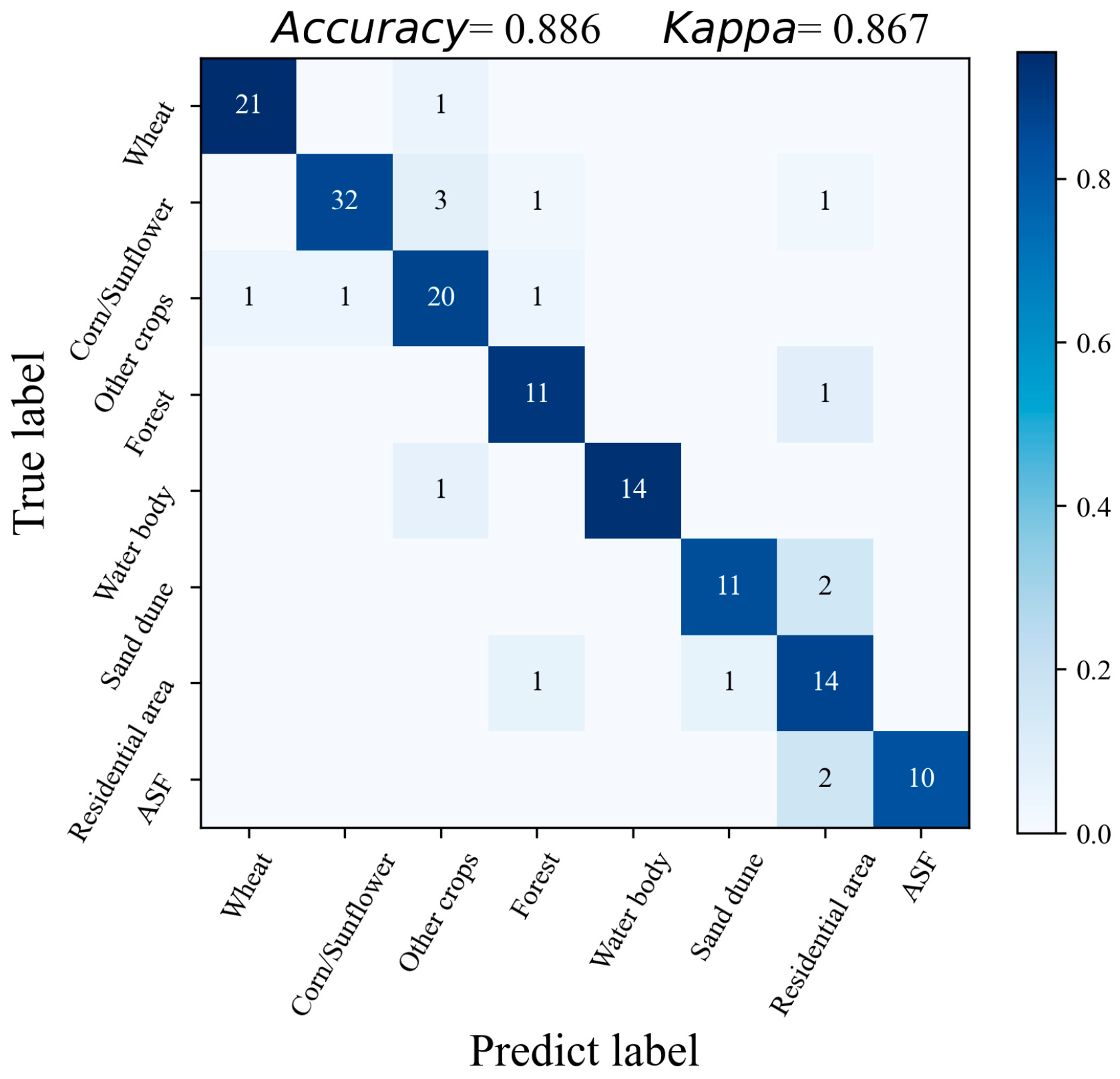
4.4. Validation of Land-Use Classification and Abandoned Farmland Detection
5. Discussion
6. Conclusions
Supplementary Materials
Author Contributions
Funding
Acknowledgments
Conflicts of Interest
References
- FAO. 2021. Available online: http://www.fao.org/soils-portal/soil-management/management-of-some-problem-soils/salt-affected-soils/more-information-on-salt-affected-soils/en/ (accessed on 31 August 2021).
- Thomas, D.S.G.; Middleton, N.J. Salinization: New perspectives on a major desertification issue. J. Arid Environ. 1993, 24, 95–105. [Google Scholar] [CrossRef]
- Konukcu, F.; Gowing, J.W.; Rose, D.A. Dry drainage: A sustainable solution to waterlogging and salinity problems in irrigation areas? Agric. Water Manag. 2006, 83, 1–12. [Google Scholar] [CrossRef]
- Vengosh, A. Salinization and Saline. Environ. Geochem. 2005, 9, 333. [Google Scholar]
- De Pascale, S.; Maggio, A.; Barbieri, G. Soil salinization affects growth, yield and mineral composition of cauliflower and broccoli. Eur. J. Agron. 2005, 23, 254–264. [Google Scholar] [CrossRef]
- Machado, R.M.A.; Serralheiro, R.P. Soil salinity: Effect on vegetable crop growth. Management practices to prevent and mitigate soil salinization. Horticulturae 2017, 3, 30. [Google Scholar] [CrossRef]
- Yuan, F.; Sawaya, K.E.; Loeffelholz, B.C.; Bauer, M.E. Land cover classification and change analysis of the Twin Cities (Minnesota) metropolitan area by multitemporal Landsat remote sensing. Remote Sens. Environ. 2005, 98, 317–328. [Google Scholar] [CrossRef]
- Carrão, H.; Gonçalves, P.; Caetano, M. Contribution of multispectral and multitemporal information from MODIS images to land cover classification. Remote Sens. Environ. 2008, 112, 986–997. [Google Scholar] [CrossRef]
- Yuan, H.; Van Der Wiele, C.F.; Khorram, S. An automated artificial neural network system for land use/land cover classification from landsat TM imagery. Remote Sens. 2009, 1, 243. [Google Scholar] [CrossRef] [Green Version]
- Wu, J.; Vincent, B.; Yang, J.; Bouarfa, S.; Vidal, A. Remote sensing monitoring of changes in soil salinity: A case study in inner Mongolia, China. Sensors 2008, 8, 7035. [Google Scholar] [CrossRef] [PubMed] [Green Version]
- Allbed, A.; Kumar, L.; Aldakheel, Y.Y. Assessing soil salinity using soil salinity and vegetation indices derived from IKONOS high-spatial resolution imageries: Applications in a date palm dominated region. Geoderma 2014, 230–231, 1–8. [Google Scholar] [CrossRef]
- Morshed, M.M.; Islam, M.T.; Jamil, R. Soil salinity detection from satellite image analysis: An integrated approach of salinity indices and field data. Environ. Monit. Assess. 2016, 188, 1–10. [Google Scholar] [CrossRef]
- Yu, B.; Shang, S. Multi-year mapping of maize and sunflower in hetao irrigation district of china with high spatial and temporal resolution vegetation index series. Remote Sens. 2017, 9, 855. [Google Scholar] [CrossRef] [Green Version]
- Gislason, P.O.; Benediktsson, J.A.; Sveinsson, J.R. Random forests for land cover classification. Pattern Recognit. Lett. 2006, 27, 294–300. [Google Scholar] [CrossRef]
- Sukawattanavijit, C.; Chen, J.; Zhang, H. GA-SVM Algorithm for Improving Land-Cover Classification Using SAR and Optical Remote Sensing Data. IEEE Geosci. Remote Sens. Lett. 2017, 14, 284–288. [Google Scholar] [CrossRef]
- Dara, A.; Baumann, M.; Kuemmerle, T.; Pflugmacher, D.; Rabe, A.; Griffiths, P.; Hölzel, N.; Kamp, J.; Freitag, M.; Hostert, P. Mapping the timing of cropland abandonment and recultivation in northern Kazakhstan using annual Landsat time series. Remote Sens. Environ. 2018, 213, 49–60. [Google Scholar] [CrossRef]
- Löw, F.; Prishchepov, A.V.; Waldner, F.; Dubovyk, O.; Akramkhanov, A.; Biradar, C.; Lamers, J.P.A. Mapping Cropland Abandonment in the Aral Sea Basin with MODIS Time Series. Remote Sens. 2018, 10, 159. [Google Scholar] [CrossRef] [Green Version]
- Yin, H.; Brandão, A.; Buchner, J.; Helmers, D.; Iuliano, B.G.; Kimambo, N.E.; Lewińska, K.E.; Razenkova, E.; Rizayeva, A.; Rogova, N.; et al. Monitoring cropland abandonment with Landsat time series. Remote Sens. Environ. 2020, 246, 111873. [Google Scholar] [CrossRef]
- Gaetano, R.; Ienco, D.; Ose, K.; Cresson, R. A two-branch CNN architecture for land cover classification of PAN and MS imagery. Remote Sens. 2018, 10, 1746. [Google Scholar] [CrossRef] [Green Version]
- Tong, X.Y.; Xia, G.S.; Lu, Q.; Shen, H.; Li, S.; You, S.; Zhang, L. Land-cover classification with high-resolution remote sensing images using transferable deep models. Remote Sens. Environ. 2020, 237, 111322. [Google Scholar] [CrossRef] [Green Version]
- Goodfellow, I.; Bengio, Y.; Courville, A.; Bengio, Y. Deep Learning; MIT Press: Cambridge, MA, USA, 2016; Volume 1. [Google Scholar]
- Kussul, N.; Lavreniuk, M.; Skakun, S.; Shelestov, A. Deep Learning Classification of Land Cover and Crop Types Using Remote Sensing Data. IEEE Geosci. Remote Sens. Lett. 2017, 14, 778–782. [Google Scholar] [CrossRef]
- Knauer, U.; von Rekowski, C.S.; Stecklina, M.; Krokotsch, T.; Minh, T.P.; Hauffe, V.; Kilias, D.; Ehrhardt, I.; Sagischewski, H.; Chmara, S.; et al. Tree species classification based on hybrid ensembles of a convolutional neural network (CNN) and random forest classifiers. Remote Sens. 2019, 11, 2788. [Google Scholar] [CrossRef] [Green Version]
- Portalés-Julià, E.; Campos-Taberner, M.; García-Haro, F.J.; Gilabert, M.A. Assessing the sentinel-2 capabilities to identify abandoned crops using deep learning. Agronomy 2021, 11, 654. [Google Scholar] [CrossRef]
- Douaoui, A.E.K.; Nicolas, H.; Walter, C. Detecting salinity hazards within a semiarid context by means of combining soil and remote-sensing data. Geoderma 2006, 134, 217–230. [Google Scholar] [CrossRef]
- Dehni, A.; Lounis, M. Remote sensing techniques for salt affected soil mapping: Application to the Oran region of Algeria. Procedia Eng. 2012, 33, 188–198. [Google Scholar] [CrossRef] [Green Version]
- Yang, Y.N.; Sheng, Q.; Zhang, L.; Kang, H.Q.; Liu, Y. Desalination of saline farmland drainage water through wetland plants. Agric. Water Manag. 2015, 156, 19–29. [Google Scholar] [CrossRef]
- Sinha, S.; Matsumoto, T.; Tanaka, Y.; Ishida, J.; Kojima, T.; Kumar, S. Solar desalination of saline soil for afforestation in arid areas: Numerical and experimental investigation. Energy Convers. Manag. 2002, 43, 15–31. [Google Scholar] [CrossRef]
- Mora, J.L.; Herrero, J.; Weindorf, D.C. Multivariate analysis of soil salination-desalination in a semi-arid irrigated district of Spain. Geoderma 2017, 291, 1–10. [Google Scholar] [CrossRef] [Green Version]
- Wang, H.W.; Fan, Y.H.; Tiyip, T. The Research of Soil Salinization Human Impact Based on Remote Sensing Classification in Oasis Irrigation Area. Procedia Environ. Sci. 2011, 10, 2399–2405. [Google Scholar] [CrossRef] [Green Version]
- Scaramuzza, P.; Barsi, J. Landsat 7 scan line corrector-off gap-filled product development. In Proceedings of the Pecora, Sioux Falls, SD, USA, 23–27 October 2005; Volume 16, pp. 23–27. [Google Scholar]
- Lobell, D.B.; Thau, D.; Seifert, C.; Engle, E.; Little, B. A scalable satellite-based crop yield mapper. Remote Sens. Environ. 2015, 164, 324–333. [Google Scholar] [CrossRef]
- Sakamoto, T.; Wardlow, B.D.; Gitelson, A.A.; Verma, S.B.; Suyker, A.E.; Arkebauer, T.J. A Two-Step Filtering approach for detecting maize and soybean phenology with time-series MODIS data. Remote Sens. Environ. 2010, 114, 2146–2159. [Google Scholar] [CrossRef]
- Likas, A.; Vlassis, N.; Verbeek, J.J. The global k-means clustering algorithm. Pattern Recognit. 2003, 36, 451–461. [Google Scholar] [CrossRef] [Green Version]
- Yang, Q.; Shi, L.; Han, J.; Yu, J.; Huang, K. A near real-time deep learning approach for detecting rice phenology based on UAV images. Agric. For. Meteorol. 2020, 287, 107938. [Google Scholar] [CrossRef]
- Otsu, N. A threshold selection method from gray-level histograms. IEEE Trans. Syst. Man. Cybern. 1979, 9, 62–66. [Google Scholar] [CrossRef] [Green Version]
- Khan, N.M.; Rastoskuev, V.V.; Sato, Y.; Shiozawa, S. Assessment of hydrosaline land degradation by using a simple approach of remote sensing indicators. Agric. Water Manag. 2005, 77, 96–109. [Google Scholar] [CrossRef]
- Gorji, T.; Sertel, E.; Tanik, A. Monitoring soil salinity via remote sensing technology under data scarce conditions: A case study from Turkey. Ecol. Indic. 2017, 74, 384–391. [Google Scholar] [CrossRef]
- Abrol, I.P.; Yadav, J.S.P.; Massoud, F.I. Salt-Affected Soils and Their Management; Food & Agriculture Organization: Rome, Italy, 1988; ISBN 9251026866. [Google Scholar]
- Crisci, C.; Ghattas, B.; Perera, G. A review of supervised machine learning algorithms and their applications to ecological data. Ecol. Modell. 2012, 240, 113–122. [Google Scholar] [CrossRef]
- Justice, C.O.; Vermote, E.; Townshend, J.R.G.; Defries, R.; Roy, D.P.; Hall, D.K.; Salomonson, V.V.; Privette, J.L.; Riggs, G.; Strahler, A.; et al. The moderate resolution imaging spectroradiometer (MODIS): Land remote sensing for global change research. IEEE Trans. Geosci. Remote Sens. 1998, 36, 1228–1249. [Google Scholar] [CrossRef] [Green Version]
- Gowing, J.W.; Wyseure, G.C.L. Dry-drainage a sustainable and cost-effective solution to waterlogging and salinisation. In Proceedings of the 5th International Drainage Workshop, Lahore, Pakistan, 8–15 February 1992; Volume 3, pp. 6–26. [Google Scholar]
- Xu, X.; Huang, G.; Qu, Z.; Pereira, L.S. Assessing the groundwater dynamics and impacts of water saving in the Hetao Irrigation District, Yellow River basin. Agric. Water Manag. 2010, 98, 301–313. [Google Scholar] [CrossRef]
- Yamaguchi, T.; Blumwald, E. Developing salt-tolerant crop plants: Challenges and opportunities. Trends Plant Sci. 2005, 10, 615–620. [Google Scholar] [CrossRef] [PubMed]


| Satellite Platform | Used Bands | The Number of Investigated Temporal Imageries | Investigated Period | ||
|---|---|---|---|---|---|
| Band Name | Wavelength (μm) | Resolution (m) | |||
| Landsat 5 TM | Band1-Blue | 0.45–0.52 | 30 | 207 | 1988–2011 |
| Band2-Green | 0.52–0.60 | 30 | |||
| Band3-Red | 0.63–0.69 | 30 | |||
| Band4-NIR | 0.76–0.90 | 30 | |||
| Band5-SWIR 1 | 1.55–1.75 | 30 | |||
| Band6-Thermal | 10.40–12.50 | 120 | |||
| Band7-SWIR 2 | 2.08–2.35 | 30 | |||
| Landsat 7 ETM+ | Band1-Blue | 0.45–0.52 | 30 | 6 | 2012 |
| Band2-Green | 0.52–0.60 | 30 | |||
| Band3-Red | 0.63–0.69 | 30 | |||
| Band4-NIR | 0.77–0.90 | 30 | |||
| Band5-SWIR 1 | 1.55–1.75 | 30 | |||
| Band6-Thermal | 10.40–12.50 | 60 | |||
| Band7-SWIR 7 | 2.09–2.35 | 30 | |||
| Landsat 8 OLI | Band2-Blue | 0.452–0.512 | 30 | 67 | 2013–2019 |
| Band3-Green | 0.533–0.590 | 30 | |||
| Band4-Red | 0.636–0.673 | 30 | |||
| Band5-NIR | 0.851–0.879 | 30 | |||
| Band6-SWIR 1 | 1.566–1.651 | 30 | |||
| Band7-SWIR 2 | 2.107–2.294 | 40 | |||
| Band10-Thermal1 | 10.6–11.19 | 100 | |||
| Sentinel 2 | Band2-Blue | 0.46–0.53 | 10 | 1 | 2019 |
| Band4-Red | 0.65–0.68 | 10 | |||
| Class | Accuracy | F1-Score | Precision | Recall |
|---|---|---|---|---|
| Wheat | 0.987 | 0.955 | 0.955 | 0.955 |
| Corn and sunflower | 0.960 | 0.914 | 0.970 | 0.865 |
| Other crops | 0.947 | 0.833 | 0.800 | 0.870 |
| Forest | 0.973 | 0.846 | 0.786 | 0.917 |
| Water body | 0.993 | 0.966 | 1.000 | 0.933 |
| Sand dune area | 0.980 | 0.880 | 0.917 | 0.846 |
| Residential area | 0.947 | 0.778 | 0.700 | 0.875 |
| Abandoned salinized farmland | 0.987 | 0.909 | 1.000 | 0.833 |
Publisher’s Note: MDPI stays neutral with regard to jurisdictional claims in published maps and institutional affiliations. |
© 2021 by the authors. Licensee MDPI, Basel, Switzerland. This article is an open access article distributed under the terms and conditions of the Creative Commons Attribution (CC BY) license (https://creativecommons.org/licenses/by/4.0/).
Share and Cite
Zhao, L.; Yang, Q.; Zhao, Q.; Wu, J. Assessing the Long-Term Evolution of Abandoned Salinized Farmland via Temporal Remote Sensing Data. Remote Sens. 2021, 13, 4057. https://doi.org/10.3390/rs13204057
Zhao L, Yang Q, Zhao Q, Wu J. Assessing the Long-Term Evolution of Abandoned Salinized Farmland via Temporal Remote Sensing Data. Remote Sensing. 2021; 13(20):4057. https://doi.org/10.3390/rs13204057
Chicago/Turabian StyleZhao, Liya, Qi Yang, Qiang Zhao, and Jingwei Wu. 2021. "Assessing the Long-Term Evolution of Abandoned Salinized Farmland via Temporal Remote Sensing Data" Remote Sensing 13, no. 20: 4057. https://doi.org/10.3390/rs13204057
APA StyleZhao, L., Yang, Q., Zhao, Q., & Wu, J. (2021). Assessing the Long-Term Evolution of Abandoned Salinized Farmland via Temporal Remote Sensing Data. Remote Sensing, 13(20), 4057. https://doi.org/10.3390/rs13204057