Abstract
Convolutional neural networks (CNNs) are the go-to model for hyperspectral image (HSI) classification because of the excellent locally contextual modeling ability that is beneficial to spatial and spectral feature extraction. However, CNNs with a limited receptive field pose challenges for modeling long-range dependencies. To solve this issue, we introduce a novel classification framework which regards the input HSI as a sequence data and is constructed exclusively with multilayer perceptrons (MLPs). Specifically, we propose a spectral-spatial MLP (SS-MLP) architecture, which uses matrix transposition and MLPs to achieve both spectral and spatial perception in global receptive field, capturing long-range dependencies and extracting more discriminative spectral-spatial features. Four benchmark HSI datasets are used to evaluate the classification performance of the proposed SS-MLP. Experimental results show that our pure MLP-based architecture outperforms other state-of-the-art convolution-based models in terms of both classification performance and computational time. When comparing with the SSSERN model, the average accuracy improvement of our approach is as high as 3.03%. We believe that our impressive experimental results will foster additional research on simple yet effective MLP-based architecture for HSI classification.
1. Introduction
With the advance of hyperspectral imaging techniques, hyperspectral imagery (HSI) presents greater resolution in both spatial and spectral dimensions [1,2]. Thanks to the abundant spectral bands (typically, hundreds of narrow contiguous channels), more fine-grained ground objects distinguishment becomes possible with their subtle spectral difference. This outstanding characteristic promotes the wide application of HSI in many fields, such as precision agriculture [2], military defense [3], and environmental governance [4].
Classification is one of the major tasks in HSI processing, which aims at distinguishing the land-cover class for different pixels. For classifying HSI, a simple and intuitive way is directly feeding hyperspectral pixels (high-dimensional vectors) into classifiers such as random forest (RF) and support vector machine (SVM) [5]. However, some challenges, such as the spectral mixing, the highly correlated spectral bands, and the complex nonlinear structure of hyperspectral data, bring difficulties to the precise classification of HSI [6]. Additionally, high-spatial-resolution remote sensing HSI usually presents high diversity in content. However, the representation ability of traditional hand-crafted features based on domain knowledge may not be enough to discriminate classes with a subtle variation [7,8].
In recent years, extracting discriminative features from high-dimensional spectral signatures has achieved great success with the utilization of deep learning [9], and HSI classification accuracy has made promising improvements. For instance, Zhou et al. [10] combined stacked autoencoders (SAEs) with a local Fisher discriminant regularization to learn compact and discriminative feature mappings with high inter-class difference and intra-class aggregation. Mou et al. [11] and Hang et al. [12] proposed to treat spectral signatures as sequential data and employed recurrent neural networks (RNNs) to learn relationships from different spectral channels, e.g., spectral correlation and band-to-band variability.
The convolutional neural network (CNN) is among the most popular networks adopted for HSI classification, which can capture contextual spatial information in an end-to-end and hierarchical manner [13,14]. Cao et al. [15] proposed a unified Bayesian framework in which a CNN coupled with Markov random fields are utilized to classify HSI. Liu et al. [16] proposed a content-guided CNN to reduce the misclassification of pixels, particularly those near the cross-classes regions. Jia et al. [17] proposed a 3D Gabor CNN in which CNN kernels are replaced with 3D Gabor-modulated kernels, to improve the robustness against the scale and orientation changes. In addition, some works proposed to integrate traditional spectral-spatial feature extraction method with CNNs, to lessen the workload of the network and mitigate the overfitting problem. For example, Aptoula et al. [18] fed stacked attribute filtered images into CNNs for spatial–spectral classification. Huang et al. [19] designed a dual-path siamese CNN to classify HSI, which uses both extended morphological profiles-based spatial information and raw pixel vector-based spectral information as inputs. Besides, considering that HSI is 3D data cube, researchers proposed to use 3D CNNs to extract discriminative features. Paoletti et al. [20] employed a 3D CNN to take full advantage of the structural characteristics of hyperspectral data and used a border mirroring strategy to effectively process border regions. Sellami et al. [21] developed a 3D convolutional encoder-decoder architecture to extract spectral-spatial features from the most informative spectral bands that are selected by an adaptive dimensionality reduction method. To reduce the model complexity of the 3D CNN, Roy et al. [22] proposed a hybrid model consisting of 2D CNN and 3D CNN. In addition, Wang et al. [23] decomposed 3D convolution kernel into three small 1D convolution kernels to reduce the number of parameters, preventing the 3D CNN from suffering the overfitting problem.
To further improve feature discrimination and HSI classification accuracy, some powerful deep networks have been developed. Li et al. [24] proposed a two-stream CNN architecture based on the squeeze-and-excitation concept, which can capture spectral, local spatial, and global spatial features simultaneously. Cao et al. [25] developed a novel residual network to promote the extraction of deep features, in which hybrid dilated convolutions are utilized to enlarge convolution kernels’ receptive field without increasing the computational complexity. Dong et al. [26] proposed a cooperative spectral–spatial attention dense network, which can emphasize salient spectral–spatial features with two cooperative attention modules. Zhang et al. [27] proposed a 3D multiscale dense network to take full advantage of features at different scales for HSI classification. In addition, the capsule neural network (CapsNet) [28], generative adversarial networks (GANs) [29], and a graph convolutional network (GCN) [30] have also been applied for HSI classification and obtained competitive performance.
Recent studies motivate a reconsideration of the image classification process from a sequence data perspective to capture long-range dependencies [31,32]. He et al. [32] proposed a multihead self-attention mechanism-based transformer for HSI classification, which can capture dependencies between any two pixels in an input region. Tolstikhin et al. [33] proposed an MLP-mixer architecture based exclusively on multilayer perceptrons (MLPs), which can obtain the global receptive field by combining matrix transposition with token-mixing projection and thus account for long-range dependencies. Subsequently, several MLP-based architectures [34,35] have been proposed. They demonstrated that neither convolutions nor self-attention are necessary for obtaining promising performance and a simpler MLP-based architecture can perform as well as the state-of-the-art convolution-based models.
In this paper, inspired by the simple yet effective design in [33], we propose a pure MLP-based architecture, called spectral-spatial MLP (SS-MLP), for high-performance HSI classification, which does not use the attention mechanism or convolutions. The SS-MLP has a very concise architecture in which matrix transposition and MLPs are utilized to achieve a global receptive field, encoding spatial and spectral information effectively. In addition to MLPs, the standard architectural components like normalization layers and skip connections are integrated in our model, in order to achieve promising performance. Experimental results on four representative HSI datasets: University of Pavia, University of Houston, Indian Pines, and HYRANK are impressive. The proposed SS-MLP can obtain higher classification accuracies with less parameters compared with other state-of-the-art convolution-based models. Moreover, it is fast to execute.
2. MLP
Figure 1 shows a multilayer perceptron (MLP) architecture, which is made up of a series of fully connected layers [36]. As can be seen, there are three types of layers, namely, the input, output, and hidden layers. The data flows from the input layer to the output layer in a feed-forward fashion. Formally, for the lth layer, let denote the input, and its output can be calculated as follows:
where and are the weights and bias at layer l and refers to the nonlinear activation function (e.g., sigmoid and rectified linear unit).
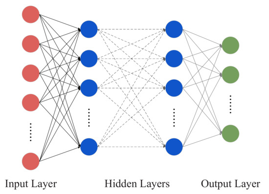
Figure 1.
Standard MLP architecture where each layer is fully connected with the adjacent layers.
Compared with the convolution-based architecture, the MLP with a global capacity is better at capturing the long-range dependencies [37]. This is because each output node is related to all input nodes. More recently, MLP-based architectures have become an appealing alternative to CNNs in computer vision [33,34,35,38,39]. For instance, Chen et al. [38] proposed a MLP-like architecture, CycleMLP, for dense prediction tasks (e.g., instance segmentation and object detection), which can deal with images with variable scales. Yu et al. [39] proposed a spatial shift MLP architecture for image classification, where spatial shift operations are employed to achieve communications between different spatial positions.
The main drawback of MLP is that it usually involves a large number of parameters. Let denote the node number at layer l. The number of parameters within an MLP is the sum of the weights and the bias between all adjacent layers, i.e., , where L denotes the layer number. Therefore, for the task of HSI classification, the MLP is usually employed at the architecture tail to perform the final classification [40]. For instance, Yang et al. [41] implemented a deep CNN with two-branch architecture for HSI classification, in which low and mid-layers are pretrained on other data sources, with a two-layer MLP performing the final classification. Xu et al. [42] proposed a novel dual-channel residual network for classifying HSI with noisy labels, which employs a noise-robust loss function to enhance model robustness and utilizes a single layer MLP for classification. To overcome this drawback, we adopt a weight sharing strategy in the proposed MLP-based architecture, which can lead to significant memory savings and will be detailed in the following Section.
3. Methodology
Figure 2 shows the architecture of the proposed SS-MLP, which takes a neighbor region (context) that is centered at the target pixel as input. Like current transformer models, such as ViT [31] and HSI-BERT [32], the proposed SS-MLP processes the HSI cubes as sequential data to encode the spatial information. The extracted region is flattened into a pixel sequence, which is then linearly projected into a new vector space using pixel embedding. The sequence of embedding vectors serves as input to the rest of the network. Several consecutive SS-MLP blocks that consist of one spatial MLP (SaMLP) and one spectral MLP (SeMLP) are used to learn discriminative spectral-spatial representations. Finally, the learned features are fed into a global average pooling layer followed by a single fully connected layer for label prediction.
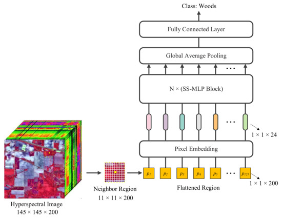
Figure 2.
An overview of the spectral-spatial MLP (SS-MLP) for HSI classification. Our SS-MLP regards input HSI patches as pixel sequences and uses MLPs with global receptive field to learn long-term dependencies. It mainly consists of pixel embedding and several SS-MLP blocks with identical architecture.
3.1. Pixel Embedding
Let be the neighbor region of the target pixel, where is the spatial size and C is the number of spectral bands. is flattened into a pixel sequence in raster scan order [32,43]. We denote the obtained pixel sequence as , where is the number of pixels.
Pixel embedding is employed to reduce the cost of computation, which transforms the sequence of pixels (high-dimensional spectral vectors) into a vector space with a smaller dimension, yielding , where is a predefined dimension. It can be viewed as one layer of the whole network. Specifically, we use a trainable linear transformation to implement pixel embedding, which works independently and identically on each pixel and can be written as:
where is a trainable weight matrix and is the bias term.
3.2. SS-MLP Block
After pixel embedding, the dimension-reduced pixel sequence, shaped as a “pixels × channels” () table, is directly fed into several SS-MLP blocks of identical architecture to learn spectral-spatial features.
The architecture of the SS-MLP block is shown in Figure 3. It simply contains two types of MLP: spatial MLP (SaMLP) and spectral MLP (SeMLP). SaMLP acts on each channel independently. It takes individual column of the table as input to capture representative spatial features. The SaMLP allows communication between pixels at different spatial locations, achieving a global receptive field in the region. In other words, each pixel is cognizant of every other pixel in the sequence. SeMLP operates on each pixel independently, allowing communication between different channels. It takes individual row of the table as input to extract discriminative spectral features. By integrating the SaMLP and SeMLP, discriminative spectral–spatial features can be extracted from HSI cubes. In addition, we adopt the skip connection mechanism of [44] to enhance information exchange between layers, which has been demonstrated to be an effective strategy for modern neural architecture design [45,46,47].
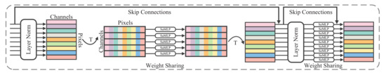
Figure 3.
The SS-MLP block. This block includes a spatial MLP (SaMLP) and a spectral MLP (SeMLP), which have similar architecture and are used to learn spatial and spectral representations separately. Note that the SaMLP is shared across different channels, while the SeMLP is shared across different pixels, achieving significant memory savings. The input and output of the SS-MLP block have the same dimension.
The SaMLP and SeMLP have similar architecture and both consist of two fully connected layers and a non-linear activation, as shown in Figure 4. We adopt the Gaussian error linear unit (GELU) [48] as the activation function, which acts on each row of its input tensor independently.
where and is the cumulative distribution function of Gaussian . In addition, the dropout regularization technique of [49] is used to prevent overfitting.
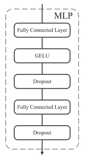
Figure 4.
The MLP architecture with two fully connected layers and a Gaussian error linear unit (GELU) [48] activation function. In addition, a dropout layer [49] is added after each fully connected layer to prevent overfitting, with a dropout rate of 50%.
Each SS-MLP block takes an input of the same size. For the sake of simplicity, here we omit block index and denote the input of each block as . The SaMLP operates on columns of (i.e., channels) and is shared across all columns, mapping . Note that we apply the same SaMLP to each row of a transposed input table to achieve the same result. The SeMLP operates on rows of (i.e., pixels), mapping . It is shared across all rows to provide the positional invariance property. For the proposed model, sharing the parameters of the SaMLP/SeMLP within each block leads to significant memory savings. In addition, since every output point is related to every input point, the SaMLP and SeMLP obtain a global receptive field in the spatial and spectral domains, which can capture richer global context information.
Mathematically, the computation process of the SS-MLP block can be written as:
where m and n are the column and row indexes, respectively, is the GELU activation function, and is the output of the SS-MLP block. The intermediate matrix obtained by the SaMLP has the same dimensions as the input and output matrices, and . refers to the Layer Normalization of [50], which is applied to speed-up the training of the model. and are the weights of the two fully connected layers in the SaMLP. and are the weights of the two fully connected layers in the SeMLP. The output of a SS-MLP block serves as the input of the next one, and so forth until the last block.
3.3. Classifying HSIs Using the Proposed SS-MLP
After processing by the last SS-MLP block, discriminative spectral-spatial features are extracted and are vectorized into a 1-D array using global average pooling and then fed into a single fully connected layer. Finally, a softmax function is attached for label prediction. Let f denote the feature vector that is fed into the softmax function. The conditional probabilities of each class can be calculated by:
where L denotes the number of ground-truth classes. The label of the target pixel is determined by the maximum probability.
Our SS-MLP model relies only on matrix multiplications, scalar non-linearities, and changes to data layout (i.e., transpositions and reshapes). Since these operations are all differentiable, the proposed model can be optimized using the standard optimization algorithms. Specifically, the learnable parameters are optimized using the Adam optimizer for 100 epochs. The learning rate is initialized with 0.001 and gradually reduced to 0.0 following a half-cosine shape schedule. The batch size is fixed to 100 and the weight decay is set as 0.0001.
4. Experimental Results
4.1. Datasets
To evaluate the effectiveness of our SS-MLP, we first conduct experiments on the University of Pavia (UP), University of Houston (UH), and Indian Pines (IP) hyperspectral benchmark datasets.
- UP: This hyperspectral scene was captured in 2001 by the reflective optics spectrographic imaging system (ROSIS)-03 airborne instrument, which covers an urban area surrounding the Engineering School of the University of Pavia in the city of Pavia, Northern Italy. The spatial dimensions of this scene are pixels, with a 1.3 m ground sampling distance (GSD). The data cube contains a total of 115 spectral reflectance bands in the wavelength range from 0.43 to 0.86 m (VNIR). Before the experiments, 12 very noisy bands were removed. Therefore, the data dimensionality is . There are mainly 9 categories of ground materials in the scene.
- UH: This hyperspectral scene was gathered by the Compact Airborne Spectrographic Imager (CASI)-1500 sensor on June 23, 2012 between 17:37:10 and 17:39:50 UTC, which covers the campus of University of Houston and the neighboring urban area in the city of Texas, United States. It consists of pixels with a GSD of 2.5 m. The considered scene contains 144 spectral reflectance bands in the wavelength range from 0.38 to 1.05 m (VNIR), forming a data cube of dimension . This dataset was provided by the 2013 IEEE Geoscience and Remote Sensing Society (GRSS) data fusion contest and has been calibrated to at-sensor spectral radiance units. There are mainly 15 categories of ground materials in this dataset.
- IP: This hyperspectral scene was acquired in 1992 by the airborne visible/ infrared imaging spectrometer (AVIRIS) sensor, which covers the agricultural Indian Pines test site in northwestern Indiana, United States. This hyperspectral scene mainly comprises crops of regular geometry and irregular forest regions. The spatial dimensions of this scene are pixels, with a 20 m GSD. In addition, it consists of 224 spectral reflectance bands in the wavelength range from 0.4 to 2.5 m, spanning the VNIR-SWIR. In our experiments, four null bands and other 20 water absorption bands (104–108, 150–163, and 220) have been removed, keeping the rest 200 bands for analysis. Therefore, the data dimensionality is . There are mainly 16 categories of ground materials in the data.
To make the proposed SS-MLP fully comparable with other spectral-spatial classification approaches reported in the literature, we use the same fixed training and test sets that are adopted by other state-of-the-art methods [51,52,53,54,55]. In other words, the number of training and test samples and their spatial locations are exactly the same with those used in previous studies. Figure 5, Figure 6 and Figure 7 depict the false color image and the spatial distribution of the fixed training and test samples for the UP, UH, and IP datasets, respectively. Table 1, Table 2 and Table 3 list the class name and the number of training and test samples on the three datasets.
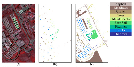
Figure 5.
ROSIS-3 University of Pavia (UP) hyperspectral dataset with 103 bands across the spectral range from 0.43 to 0.86 m. (a) False-color composite image for the hyperspectral data using bands 81, 21, and 41 as R, G, B, respectively. (b) Training samples. (c) Test samples.
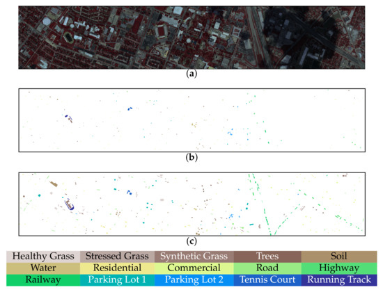
Figure 6.
CASI-1500 University of Houston (UH) hyperspectral dataset with 144 bands across the spectral range from 0.38 to 1.05 m. (a) False-color composite image for the hyperspectral data using bands 108, 28, and 27 as R, G, B, respectively. (b) Training samples. (c) Test samples.
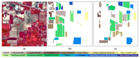
Figure 7.
AVIRIS Indian Pines (IP) hyperspectral dataset with 200 bands across the spectral range from 0.4 to 2.5 m. (a) False-color composite image for the hyperspectral data using bands 37, 20, and 12 as R, G, B, respectively. (b) Training samples. (c) Test samples.

Table 1.
Number of samples on the UP dataset. Note that the standard training and test sets are used.
Table 2.
Number of samples on the UH dataset. Note that the standard training and test sets are used.
Table 3.
Number of samples on the IP dataset. The spatially disjoint training and test sets are used.
4.2. Evaluation Metrics
The overall accuracy (OA), average accuracy (AA), Kappa coefficient, and F1-score are used for quantitative analysis. To demonstrate the stability of our results, each experiment is conducted five times across different seeds and the mean and standard variation of the scores are reported.
4.3. Parameter Analysis
The model complexity of the SS-MLP is controlled by the network depth, i.e., the number of SS-MLP blocks, and the embedding dimension D. Considering that low complexity leads to underfitting and high complexity may result in the waste of computational resources and overfitting, we aim to find the smallest model depth and embedding dimension without incurring underfitting.
The OA of SS-MLP with different model depths is summarized in Table 4. As can be seen, the best OAs are achieved when the model depth is set to 3, 2, and 1 for the UP, UH, and IP datasets, respectively. Table 5 lists the OA of SS-MLP with different embedding dimensions. Note that when the embedding dimension is set to 24, the OA index reaches the maximum value on the three datasets.
Table 4.
OA (%) of SS-MLP with different model depths. Note that we use the number of SS-MLP blocks to represent model depth. The best results are highlighted in bold font.
Table 5.
OA (%) of SS-MLP with different embedding dimension D. For our model, pixel embedding is used to reduce the redundant spectral information and the default value of D is 24. The best results are highlighted in bold font.
4.4. Comparison Methods
Next, we compare our SS-MLP with the following spectral-spatial methods:
- DenseNet [56]: A deep&dense CNN which employs shortcut connections between layers to avoid the vanishing model gradient and enhance network generalization. It exploits both low-level and high-level features extracted from HSI data for classification.
- FDMFN [57]: A fully dense multiscale fusion network which exploits the complementary and correlated multiscale features from different convolution layers for HSI classification. With the fully dense connectivity pattern, any two layers in the network are connected to ensure maximum information flow.
- MSRN [58]: A multiscale residual network which integrates multiscale filter banks ( and filters) into depthwise convolution operations, in order to not only learn multiscale information from HSI data but also reduce the computational cost of the network.
- DPRN [59]: A deep pyramidal residual network which is made up several pyramidal bottleneck residual blocks. As the network depth increases, more feature maps are generated to improve the diversity of high-level spectral–spatial features.
- SSSERN [60]: A spatial–spectral squeeze-and-excitation residual network which extracts distinguishable features through spatial and spectral attention mechanisms, emphasizing meaningful features and suppressing unnecessary ones in the spatial and spectral domains simultaneously.
For the compared networks, their default parameter configurations are used. The training details of the compared methods are summarized in Appendix A. To make a fair comparison between different approaches, the input 3D HSI patches’ spatial size is fixed to , following the set up of [56,59,60]. All the networks are implemented on the PyTorch platform using a personal computer with a RTX 2080 GPU.
4.5. Comparison Results
Table 6, Table 7 and Table 8 present the quantitative classification results for the UP, UH, and IP datasets, respectively. As can be seen, the proposed SS-MLP consistently provides superior performances in terms of three overall indices: OA, AA, and Kappa, over the other methods applied to all three datasets.
Table 6.
Classification accuracies (%) on the UP dataset. The input HSI patch size is fixed to for different models. SS-MLP achieves higher OA score while spending less time than other compared methods. “M” and “s” indicate millions and seconds. The best results are highlighted in bold font.
Table 7.
Classification accuracies (%) on the UH dataset. The input HSI patch size is fixed to for different models. SS-MLP achieves higher overall accuracies while using fewer parameters than other compared methods. “M” and “s” indicate millions and seconds. The best results are highlighted in bold font.
Table 8.
Classification accuracies (%) on the IP dataset. The input HSI patch size is fixed to for different models. SS-MLP achieves higher overall accuracies while using fewer parameters than other compared methods. “M” and “s” indicate millions and seconds. The best results are highlighted in bold font.
Focusing on the UP dataset, the SS-MLP achieves OA, AA, and Kappa values of 96.23%, 95.48%, and 94.93%, respectively, while the second-best model (SSSERN) obtains 94.63%, 94.53%, and 92.71%, respectively. The promotions of the OA, AA, and Kappa values are 1.60%, 0.95%, and 2.22%, respectively. However, the F1-score obtained by our model is slightly lower than that achieved by SSSERN (only 0.24% less). Regarding the UH dataset, in comparison with the SSSERN model, our SS-MLP achieves 0.87%, 0.46%, 0.92%, and 0.70% gains in terms of OA, AA, Kappa, and F1-score, respectively.
With the IP dataset, our model shows 4.17%, 2.28%, 3.68%, 4.09%, and 4.65% improvements (in terms of OA) over DenseNet, FDMFN, MSRN, DPRN, and SSSERN, respectively. Note that the F1-score obtained by our SS-MLP is as high as 71.46%, which is 8.33% point higher than that of SSSERN (63.13%). The reason for the remarkable promotions may be that the proposed SS-MLP with a global receptive filed is able to achieve better reasoning over a longer context, which is suitable for processing IP scene with larger smooth regions (e.g., large area of farmland). As for the UP and UH datasets, they have more detailed regions and the local detail information is important. Therefore, we obtain limited improvements for these two datasets.
Regarding the computational complexity, we compare the number of parameters and runtimes for different networks. As can be observed from Table 6, Table 7 and Table 8, the SS-MLP contains considerably fewer parameters than the DenseNet, FDMFN, DPRN, and SSSERN. Moreover, it is the fastest classification model. Consider the UP dataset. Our SS-MLP contains 41.5, 9.0, 32.7, and 2.5 times fewer parameters than the DenseNet, FDMFN, DPRN, and SSSERN, respectively. Although MSRN have approximately the same number of parameters as our SS-MLP, it requires more execution times (101.48 s vs. 90.66 s). Similar results can be seen on the UH and IP datasets.
For the UP and UH datasets, the differences between the second-best model SSSERN and the proposed SS-MLP are 1.60 (94.63 ± 0.96 vs. 96.23 ± 0.51) and 0.87 (84.99 ± 0.45 vs. 85.86 ± 0.96), respectively. As for the IP dataset, the difference between the second-best model FDMFN and our SS-MLP is 2.28 (66.37 ± 2.78 vs. 68.65 ± 0.65). Although our SS-MLP’s improvements are not very significant on the UH dataset, it requires the fewest number of parameters and takes the shortest time to achieve satisfactory accuracy, which demonstrates the efficiency of our method.
DenseNet and DPRN have millions of parameters, which result in a high probability of incurring the phenomenon of overfitting. This is because DenseNet has a deep architecture which consists of 22 inner convolution blocks, while DPRN uses larger convolution kernels (i.e., instead of the widely used ) to increase the receptive field. In addition, during the feature extraction process, DenseNet adopts pooling operation to reduce data variance and computation complexity. However, the spatial resolution of learned feature maps is also reduced, resulting in the detail information loss. This is because HSI classification models (e.g., DenseNet) usually take image patches as input, which have a small spatial size (e.g., ). Due to the spatial detail information loss and the high probability of overfitting, DenseNet performs relatively poor on the three datasets. FDMFN and MSRN can utilize contextual information at different scales for classification, achieving satisfactory performance. When learning spectral-spatial features, SSSERN keeps the spatial size of input hyperspectral data fixed to avoid spatial information loss. In addition, it uses spectral attention modules to emphasize useful bands for classification and suppress useless bands. Moreover, SSSERN utilizes spatial attention modules to emphasize pixels that are useful for classification (i.e., highlighting pixels from the same class as the center pixel) and suppress useless pixels. In this way, SSSERN is able to extract discriminative spectral-spatial features from the HSI cubes and achieves promising classification performance. However, the CNN-based models (i.e., DenseNet, FDMFN, MSRN, DPRN, and SSSERN) have limited receptive field, which makes the learned features focusing more on local information and may result in the misclassifications inside objects. As for the proposed SS-MLP, it is constructed based on MLPs with global receptive field, which can capture long-range dependencies. In addition, to avoid detail information loss, we do not use any downsampling operation during the feature extraction phase. Moreover, due to the weight sharing strategy, our SS-MLP architecture is lightweight, which can alleviate the overfitting problem and is suitable for HSI classification task with limited training samples. Therefore, our model achieves competitive performance in comparison with other methods.
Figure 8, Figure 9 and Figure 10 provide the classification maps generated by different approaches on the three datasets. As can be observed, the SS-MLP produces well-defined classification maps in terms of border delineation. For the UH dataset, the classification map obtained by our SS-MLP is more aligned with ground object boundaries, particularly for the “Railway” class. Figure 11 shows the classification maps for the “Railway” class obtained by different methods. As can be observed, the DenseNet, FDMFN, MSRN, and DPRN misidentify parts of the middle area of “Railway” as “Parking Lot 2” (denoted by blue color). For the SSSERN, it misidentifies parts of the middle area of “Railway” as “Road”. The reason for the misclassifications may be that these five convolution-based methods have limited receptive filed and thus focus more on local information, resulting in the misclassifications inside large scale objects. However, the proposed SS-MLP with a global receptive filed can capture long-range spatial interactions, which is better at classifying objects from a global perspective. That may be the reason why the proposed SS-MLP achieves a better classification performance on the “Railway” class.
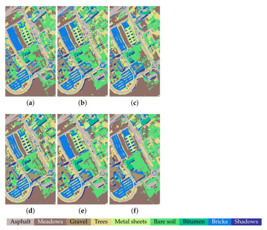
Figure 8.
Classification maps on the UP dataset. (a) DenseNet, OA = 91.33%. (b) FDMFN, OA = 91.63%. (c) MSRN, OA = 91.94%. (d) DPRN, OA = 92.28%. (e) SSSERN, OA = 94.63%. (f) SS-MLP, OA = 96.23%.
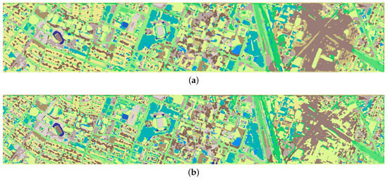
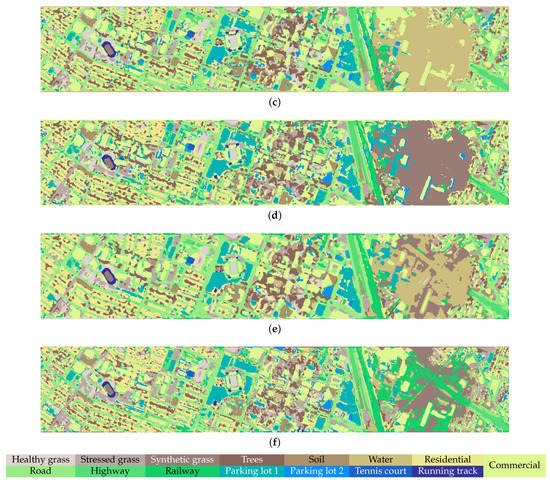
Figure 9.
Classification maps on the UH dataset. (a) DenseNet, OA = 82.84%. (b) FDMFN, OA = 84.04%. (c) MSRN, OA = 84.91%. (d) DPRN, OA = 82.64%. (e) SSSERN, OA = 84.99%. (f) SS-MLP, OA = 85.86%.

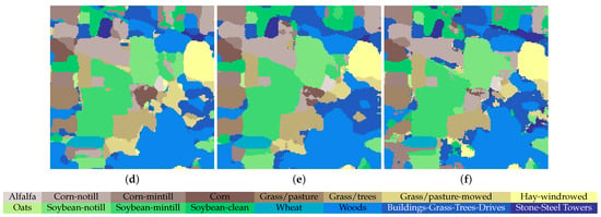
Figure 10.
Classification maps on the IP dataset. (a) DenseNet, OA = 64.48%. (b) FDMFN, OA = 66.37%. (c) MSRN, OA = 64.97%. (d) DPRN, OA = 64.56%. (e) SSSERN, OA = 64.00%. (f) SS-MLP, OA = 68.65%.
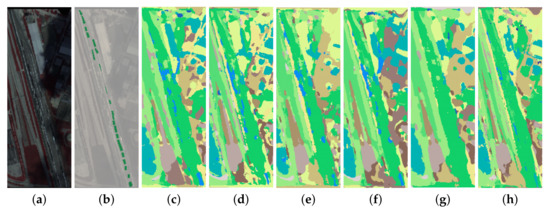
Figure 11.
Classification maps for the “Railway” class obtained by different methods on the UH dataset. (a) False color image. (b) Ground reference map for “Railway” class. (c) DenseNet. (d) FDMFN. (e) MSRN. (f) DPRN. (g) SSSERN. (h) SS-MLP.
In addition, for the IP dataset, the classification accuracies obtained by our method are similar to that achieved by SSSERN in most categories. However, our SS-MLP achieves significant improvements over SSSERN in the “Soybean-clean” category (58.98 ± 9.36 vs. 20.89 ± 6.41). The “Soybean-clean”, “Soybean-notill”, and “Soybean-mintill” categories are similar, which make accurate separation difficult. For “Soybean-clean” category, all methods obtain poor accuracy (lower than 60%). However, the proposed SS-MLP can achieve a better classification performance compared with other methods, possibly since global information is important for accurately classifying this category with large-scale areas. Without the help of global receptive field, pixels inside large objects are usually mistaken as other objects with high similarity. Figure 12 shows the features learned by SSSERN model and the proposed SS-MLP. Note that the final spectral-spatial features extracted before global average pooling are displayed. As can be seen, our SS-MLP tends to focus on pixels in different areas of the input HSI patch and hence can reason in an enlarged spatial range and from a global prospective. However, SSSERN pays more attention on local information. Therefore, we hypothesize that the success of detecting this category arises from the SS-MLP’s characteristic of global receptive field.
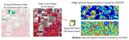
Figure 12.
Feature maps learned by SSSERN and the proposed SS-MLP for “Soybean-clean” class from the IP dataset. SSSERN with local receptive field focuses more on local information, while our SS-MLP with global receptive field can pay attention to all the pixels in the input HSI patch.
5. Discussion
5.1. Ablation Analysis of the Proposed SS-MLP
The proposed SS-MLP uses the skip connection mechanism, layer normalization, and a 50% dropout regularization for improving the training process. To demonstrate the effectiveness of our model, we construct a baseline network by eliminating skip connection, layer normalization, and dropout regularization from the SS-MLP. As can be seen from Table 9, the baseline network obtains poor classification performance. Specifically, the OA scores obtained by the baseline model are 56.61%, 79.92%, and 62.60% on the UP, UH, and IP datasets, respectively.
Table 9.
Ablation analysis of SS-MLP for understanding the contribution of different components in the architecture, including skip connection, layer normalization, and dropout regularization. We can find all these three components have positive contributions to the classification performance. The best results are highlighted in bold font.
To improve the classification performance of the baseline network, skip connection mechanism is first introduced, which can enhance the information exchange between layers and reduce the training difficulty [44]. As can be observed from Table 9, the OA scores’ improvements obtained by utilizing skip connection mechanism are 33.73%, 2.23%, and 0.55% on the three datasets, which demonstrate that improving the information flow is useful to enhance the HSI classification accuracy. In addition, we further adopt layer normalization [50] to reduce the internal covariate shift during network training, which can speed up the training phase and benefit generalization. As can be seen, the increases of OA scores obtained by the combination of layer normalization and skip connection are 37.52% on the UP dataset, 4.05% on the UH dataset, and 4.25% on the IP dataset, which demonstrates that the utilization of layer normalization also plays a positive role in improving classification accuracy. Besides, dropout regularization is used to improve the training process. Specifically, during the training phase, it randomly deactivates a percentage of neurons, that is, setting the output of each neuron to zero with a probability. By dropping neurons randomly, diverse neural networks are formed in different training epochs, which can reduce the co-adaptation of hidden units and force the network to learn more robust features [49]. The most commonly used dropout rate is 50%. From the observation of Table 9, we can find that the network with dropout regularization can achieve better performance on all three datasets. This suggests that dropout regularization is beneficial to enhance the classification performance.
To sum up, the utilization of different techniques can effectively obtain different degrees of improvement in the performance. When using all these three techniques, the SS-MLP performs the best on all three HSI datasets. Compared with the baseline network, the OA scores’ enhancements achieved by our SS-MLP are as high as 39.62% on the UP dataset, 5.94% on the UH dataset, and 6.05% on the IP dataset, which demonstrates that the SS-MLP architecture designed in this article is effective for the task of HSI classification.
5.2. Impact of SeMLP and SaMLP
Considering that each pixel in hyperspectral imagery covers a spatial region on the surface of the Earth, hyperspectral pixels tend to have mixed spectral signatures. The presence of mixed pixels and the environmental interferes like atmospheric and geometric distortions often lead to: (1) Spectral signatures that belong to the same land-cover type may be different. (2) Spectral signatures belonging to different classes may be similar. Therefore, methods that focus only on the spectral information cannot provide satisfactory classification accuracy. By exploiting the spatial contextual information such as textures, geometrical structures and neighboring relationships, spectral-spatial methods have proven to be an effective way to reduce the classification uncertainty and increase the classification accuracies.
In this paper, the SeMLP is used to learn discriminative spectral features, and the SaMLP that can capture relationships between any two pixels in an input region is used to extract informative global spatial features. To demonstrate the effectiveness of the integration of SaMLP and SeMLP in our SS-MLP, we also test the networks that only consist of the SaMLPs and the ones that only contain SeMLPs.
Since the spectral representations learned by SeMLP are complementary to the spatial features learned by the SaMLP, the proposed SS-MLP with both SeMLP and SaMLP consistently obtain higher OA values than the networks with only SeMLP or SaMLP, as can be seen from Table 10. On the UP dataset, the OA of our SS-MLP is 96.23%, and it is 8.57% and 2.98% higher than the OA obtained by the network without SaMLP and the one without SeMLP, respectively. For the UH dataset, combination of both SaMLP and SeMLP could increase the OA value by 0.56% and 2.05% compared to the network without SaMLP or SeMLP. As for the IP dataset, removing SaMLP and SeMLP will result in a 5.50% and 2.06% decrease in OA score, respectively. These results demonstrate the importance of both the SaMLP and SeMLP in SS-MLP.
Table 10.
OA (%) of SS-MLP with different architectures. Note that the proposed SS-MLP consists of both SeMLP and SaMLP. The best results are highlighted in bold font.
5.3. Impact of Activation Function
For the proposed SS-MLP model, we adopt the Gaussian error linear unit (GELU) [48] instead of the widely used rectified linear unit (ReLU) as the activation function. The reason is that the use of GELU activation function promotes SS-MLP’s classification performance slightly on the UP and UH datasets, as can be seen from Table 11.
Table 11.
OAs (%) of our SS-MLP with different activation functions on the three datasets.
5.4. Analysis of Learning Curves of SS-MLP
Figure 13 presents the learning curves of our SS-MLP, including the loss and accuracy of training and validation for all the three datasets. Here, 10% of samples per class are randomly selected from the training set as validation samples, and the rest 90% are used for network training. Note that in this paper we follow the widely-adopted training protocol and set the training epochs to 100. However, from Figure 13, one can see that our SS-MLP is converged almost around 50 epochs, which means that the time cost of our model can be further reduced by using fewer training epochs.
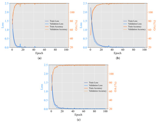
Figure 13.
Learning curves of the proposed SS-MLP on (a) UP, (b) UH, and (c) IP datasets. As can be observed, our model has the characteristic of fast convergence, which can converge at a stable minimum within as few as 50 epochs for these three datasets.
5.5. Analysis of General Applicability
In this section, we further investigate the general applicability and performance of the SS-MLP on a recently released HYRANK hyperspectral benchmark dataset. The HYRANK datasets contains five hyperspectral scenes: Dioni, Loukia, Erato, Nefeli, and Kiriki, where the ground reference maps of Dioni and Loukia scenes are available. Researchers usually use Dioni scene as training set and Loukia scene as test set. Both the Dioni and Loukia scenes were acquired by the Hyperion sensor on the Earth Observing-1 satellite with 176 spectral bands and a GSD of 30 m. The spatial size of Dioni scene is . The spatial size of Loukia scene is . Both of them contain seven land-cover classes: Dense Urban Fabric, Non-Irrigated Arable Land, Olive Groves, Dense Sclerophyllous Vegetation, Sparse Sclerophyllous Vegetation, Sparsely Vegetated Areas, and Water. HYRANK benchmark dataset is challenging since it has spatially disjoint training and test sets. Besides, due to the limited spatial resolution (30 m), the highly mixed pixels also poses a great challenge to accurate classification of land-cover types. From Table 12, it can be seen that the proposed SS-MLP still obtains improved performance compared with other methods. In comparison with the second-best model (DPRN), our SS-MLP improves the OA by 1.08%, using approximately 53× fewer parameters. The HYRANK dataset and the classification maps obtained by different methods are displayed in the Appendix B.
Table 12.
Classification accuracies of different approaches on the HYRANK dataset. “M” indicates millions. The best results are highlighted in bold font.
The experimental outcomes on the four benchmark datasets demonstrate the effectiveness of the proposed SS-MLP. It should be noted that owing to the weight sharing strategy, the number of parameters required by our model is considerably fewer than that needed by other deep CNN models. Take the UH dataset as an example, DenseNet (1.66 M) and DPRN (1.98 M) require millions of parameters, while our SS-MLP only needs 40 K parameters. In addition, although the SSSERN and the proposed model obtain similar classification accuraices on the UH dataset, our SS-MLP needs 4× fewer parameters, being approximately 2× faster. These results demonstrate that the proposed SS-MLP can achieve competitive performance compared with the state-of-the-art methods, but requiring fewer parameters to be adjusted and less running time.
Our SS-MLP uses matrix transposition and MLPs to achieve both spectral and spatial perception in global receptive field. However, the local features that can be captured by CNNs with local receptive field is important for distinguishing small scale objects. Therefore, how to effectively embed local information in our SS-MLP architecture requires further investigation.
6. Conclusions
In this article, a novel deep learning architecture based entirely on MLPs is presented for HSI classification. The proposed SS-MLP uses two consecutive MLPs, i.e., SaMLP and SeMLP, to learn spatial and spectral representations in the global receptive filed. These two types of MLPs are interleaved to enable information interaction between spectral and spatial domains. Furthermore, weight sharing within the SS-MLP block significantly enhances memory savings. Experiments conducted on four benchmark HSI datasets demonstrate that the proposed SS-MLP can yield competitive results with less parameters compared with several state-of-the-art approaches.
In the future, we will conduct additional experiments to investigate the general applicability and performance of the SS-MLP across many different HSI datasets. In addition, we will consider integrating band selection with the proposed SS-MLP, so as to suppress useless bands and emphasize informative ones for efficient HSI classification.
Author Contributions
Conceptualization, Z.M.; methodology, Z.M.; software, Z.M.; writing—original draft preparation, Z.M.; writing—review and editing, Z.M.; validation, F.Z. and M.L.; Funding Acquisition, F.Z. All authors have read and agreed to the published version of the manuscript.
Funding
This research was funded in part by the New Star Team of Xi’an University of Posts & Telecommunications under Grant xyt2016-01, in part by the Program of Qingjiang Excellent Young Talents, Jiangxi University of Science and Technology under Grant JXUSTQJYX2020019, in part by the Natural Science Basic Research Plan in Shaanxi Province of China under Grant 2021JM-461, and in part by the National Natural Science Foundation of China under Grant 62071378, Grant 61901198, and Grant 62071379.
Institutional Review Board Statement
Not applicable.
Informed Consent Statement
Not applicable.
Data Availability Statement
The UP dataset is available at: http://dase.grss-ieee.org. The UH dataset is available at: https://hyperspectral.ee.uh.edu/. The IP hyperspectral data is available at http://www.ehu.eus/ccwintco/index.php?title=Hyperspectral_Remote_Sensing_Scenes and the corresponding spatially disjoint training and test sets can be found at: https://zhe-meng.github.io/. The HYRANK dataset is available at: https://www2.isprs.org/commissions/comm3/wg4/hyrank/. All these links can be accessed on 1 October 2021.
Acknowledgments
We gratefully thank the Associate Editor and the four Anonymous Reviewers for their outstanding comments and suggestions, which greatly helped us to improve the technical quality and presentation of our work.
Conflicts of Interest
The authors declare no conflict of interest.
Appendix A. Training Details of the Compared Methods
In order to recover the results of the compared methods, we use the training protocols reported in the corresponding references. Table A1 summarizes the training details of the compared approaches. DenseNet [56] and SSSERN [60] follow the widely-adopted training protocol. The training procedure lasts for 100 epochs, using the Adam optimizer with a batch size of 100 samples. The learning rate is set to 0.001. Note that in accordance with [57], a half-cosine shape learning rate schedule is adopted for FDMFN, which starts from 0.001 and gradually reduces to 0.0. As for DPRN, the learning rate is set to 0.1 from epochs 1 to 149 and to 0.01 from epochs 150 to 200, according to the setup in [59]. Besides, it should be noted that MSRN’s learning rate is set to 0.001 instead of the default 0.01 [58], because we found that MSRN can achieve better classification performance with a smaller learning rate.
Table A1.
Training details for different compared methods. SGD refers to the Stochastic Gradient Descent optimizer.
Table A1.
Training details for different compared methods. SGD refers to the Stochastic Gradient Descent optimizer.
| Models | Learning Rate | Epoch | Optimizer | Batch Size | Weight Decay |
|---|---|---|---|---|---|
| DenseNet [56] | 0.001 | 100 | Adam | 100 | 0.0001 |
| FDMFN [57] | 0.001 | 100 | Adam | 100 | 0.0001 |
| MSRN [58] | 0.001 | 120 | Adam | 64 | 0.0001 |
| DPRN [59] | 0.1 | 200 | SGD | 100 | 0.0001 |
| SSSERN [60] | 0.001 | 100 | Adam | 100 | 0.0001 |
Appendix B. Classification Maps for the HYRANK Dataset

Figure A1.
Hyperion HYRANK dataset with 176 spectral bands. It is worth noting that the number of training and test samples per class are reported in brackets. (a) False-color composite image for the Dioni training set using bands 23, 11, and 7 as R, G, B, respectively. (b) Ground reference map for the Dioni training set. (c) False-color composite image for the Loukia test set using bands 23, 11, and 7 as R, G, B, respectively. (d) Ground reference map for the Loukia test set. (e) DenseNet, OA = 48.23%. (f) FDMFN, OA = 49.95%. (g) MSRN, OA = 47.73%. (h) DPRN, OA = 52.40%. (i) SSSERN, OA = 48.48%. (j) SS-MLP, OA = 53.48%.
References
- Tai, X.; Li, M.; Xiang, M.; Ren, P. A mutual guide framework for training hyperspectral image classifiers with small data. IEEE Trans. Geosci. Remote Sens. 2021, 1–17. [Google Scholar] [CrossRef]
- Hu, X.; Zhong, Y.; Wang, X.; Luo, C.; Zhao, J.; Lei, L.; Zhang, L. SPNet: Spectral patching end-to-end classification network for UAV-borne hyperspectral imagery with high spatial and spectral resolutions. IEEE Trans. Geosci. Remote Sens. 2021, 1–17. [Google Scholar] [CrossRef]
- Shimoni, M.; Haelterman, R.; Perneel, C. Hypersectral imaging for military and security applications: Combining myriad processing and sensing techniques. IEEE Geosci. Remote Sens. Mag. 2019, 7, 101–117. [Google Scholar] [CrossRef]
- Han, Y.; Gao, Y.; Zhang, Y.; Wang, J.; Yang, S. Hyperspectral sea ice image classification based on the spectral-spatial-joint feature with deep learning. Remote Sens. 2019, 11, 2170. [Google Scholar] [CrossRef] [Green Version]
- Ghamisi, P.; Plaza, J.; Chen, Y.; Li, J.; Plaza, A.J. Advanced spectral classifiers for hyperspectral images: A review. IEEE Geosci. Remote Sens. Mag. 2017, 5, 8–32. [Google Scholar] [CrossRef] [Green Version]
- Wang, X.; Tan, K.; Du, Q.; Chen, Y.; Du, P. Caps-TripleGAN: GAN-assisted CapsNet for hyperspectral image classification. IEEE Trans. Geosci. Remote Sens. 2019, 57, 7232–7245. [Google Scholar] [CrossRef]
- Lu, B.; Dao, P.D.; Liu, J.; He, Y.; Shang, J. Recent advances of hyperspectral imaging technology and applications in agriculture. Remote Sens. 2020, 12, 2659. [Google Scholar] [CrossRef]
- Jia, J.; Chen, J.; Zheng, X.; Wang, Y.; Guo, S.; Sun, H.; Jiang, C.; Karjalainen, M.; Karila, K.; Duan, Z.; et al. Tradeoffs in the spatial and spectral resolution of airborne hyperspectral imaging systems: A crop identification case study. IEEE Trans. Geosci. Remote Sens. 2021, 1–18. [Google Scholar] [CrossRef]
- LeCun, Y.; Bengio, Y.; Hinton, G. Deep learning. Nature 2015, 521, 436–444. [Google Scholar] [CrossRef]
- Zhou, P.; Han, J.; Cheng, G.; Zhang, B. Learning compact and discriminative stacked autoencoder for hyperspectral image classification. IEEE Trans. Geosci. Remote Sens. 2019, 57, 4823–4833. [Google Scholar] [CrossRef]
- Mou, L.; Ghamisi, P.; Zhu, X.X. Deep recurrent neural networks for hyperspectral image classification. IEEE Trans. Geosci. Remote Sens. 2017, 55, 3639–3655. [Google Scholar] [CrossRef] [Green Version]
- Hang, R.; Liu, Q.; Hong, D.; Ghamisi, P. Cascaded recurrent neural networks for hyperspectral image classification. IEEE Trans. Geosci. Remote Sens. 2019, 57, 5384–5394. [Google Scholar] [CrossRef] [Green Version]
- Imani, M.; Ghassemian, H. An overview on spectral and spatial information fusion for hyperspectral image classification: Current trends and challenges. Inf. Fusion 2020, 59, 59–83. [Google Scholar] [CrossRef]
- Vali, A.; Comai, S.; Matteucci, M. Deep learning for land use and land cover classification based on hyperspectral and multispectral earth observation data: A review. Remote Sens. 2020, 12, 2495. [Google Scholar] [CrossRef]
- Cao, X.; Zhou, F.; Xu, L.; Meng, D.; Xu, Z.; Paisley, J. Hyperspectral image classification with Markov random fields and a convolutional neural network. IEEE Trans. Image Process. 2018, 27, 2354–2367. [Google Scholar] [CrossRef] [Green Version]
- Liu, Q.; Xiao, L.; Yang, J.; Chan, J.C.W. Content-guided convolutional neural network for hyperspectral image classification. IEEE Trans. Geosci. Remote Sens. 2020, 58, 6124–6137. [Google Scholar] [CrossRef]
- Jia, S.; Liao, J.; Xu, M.; Li, Y.; Zhu, J.; Sun, W.; Jia, X.; Li, Q. 3-D Gabor convolutional neural network for hyperspectral image classification. IEEE Trans. Geosci. Remote Sens. 2021, 1–16. [Google Scholar] [CrossRef]
- Aptoula, E.; Ozdemir, M.C.; Yanikoglu, B. Deep learning with attribute profiles for hyperspectral image classification. IEEE Geosci. Remote Sens. Lett. 2016, 13, 1970–1974. [Google Scholar] [CrossRef]
- Huang, L.; Chen, Y. Dual-path siamese CNN for hyperspectral image classification with limited training samples. IEEE Geosci. Remote Sens. Lett. 2020, 18, 518–522. [Google Scholar] [CrossRef]
- Paoletti, M.E.; Haut, J.M.; Plaza, J.; Plaza, A. A new deep convolutional neural network for fast hyperspectral image classification. ISPRS J. Photogramm. Remote. Sens. 2018, 145, 120–147. [Google Scholar] [CrossRef]
- Sellami, A.; Farah, M.; Farah, I.R.; Solaiman, B. Hyperspectral imagery classification based on semi-supervised 3-D deep neural network and adaptive band selection. Expert Syst. Appl. 2019, 129, 246–259. [Google Scholar] [CrossRef]
- Roy, S.K.; Krishna, G.; Dubey, S.R.; Chaudhuri, B.B. HybridSN: Exploring 3-D–2-D CNN feature hierarchy for hyperspectral image classification. IEEE Geosci. Remote Sens. Lett. 2019, 17, 277–281. [Google Scholar] [CrossRef] [Green Version]
- Wang, W.; Dou, S.; Wang, S. Alternately updated spectral–spatial convolution network for the classification of hyperspectral images. Remote Sens. 2019, 11, 1794. [Google Scholar] [CrossRef] [Green Version]
- Li, X.; Ding, M.; Pižurica, A. Deep feature fusion via two-stream convolutional neural network for hyperspectral image classification. IEEE Trans. Geosci. Remote Sens. 2019, 58, 2615–2629. [Google Scholar] [CrossRef] [Green Version]
- Cao, F.; Guo, W. Deep hybrid dilated residual networks for hyperspectral image classification. Neurocomputing 2020, 384, 170–181. [Google Scholar] [CrossRef]
- Dong, Z.; Cai, Y.; Cai, Z.; Liu, X.; Yang, Z.; Zhuge, M. Cooperative spectral–spatial attention dense network for hyperspectral image classification. IEEE Geosci. Remote Sens. Lett. 2020, 18, 866–870. [Google Scholar] [CrossRef]
- Zhang, C.; Li, G.; Du, S. Multi-scale dense networks for hyperspectral remote sensing image classification. IEEE Trans. Geosci. Remote Sens. 2019, 57, 9201–9222. [Google Scholar] [CrossRef]
- Xu, Q.; Wang, D.; Luo, B. Faster multiscale capsule network with octave convolution for hyperspectral image classification. IEEE Geosci. Remote Sens. Lett. 2020, 18, 361–365. [Google Scholar] [CrossRef]
- Wang, W.Y.; Li, H.C.; Deng, Y.J.; Shao, L.Y.; Lu, X.Q.; Du, Q. Generative adversarial capsule network with ConvLSTM for hyperspectral image classification. IEEE Geosci. Remote Sens. Lett. 2020, 18, 523–527. [Google Scholar] [CrossRef]
- Mou, L.; Lu, X.; Li, X.; Zhu, X.X. Nonlocal graph convolutional networks for hyperspectral image classification. IEEE Trans. Geosci. Remote Sens. 2020, 58, 8246–8257. [Google Scholar] [CrossRef]
- Dosovitskiy, A.; Beyer, L.; Kolesnikov, A.; Weissenborn, D.; Zhai, X.; Unterthiner, T.; Dehghani, M.; Minderer, M.; Heigold, G.; Gelly, S.; et al. An image is worth 16x16 words: Transformers for image recognition at scale. arXiv 2020, arXiv:2010.11929. [Google Scholar]
- He, J.; Zhao, L.; Yang, H.; Zhang, M.; Li, W. HSI-BERT: Hyperspectral image classification using the bidirectional encoder representation from transformers. IEEE Trans. Geosci. Remote Sens. 2019, 58, 165–178. [Google Scholar] [CrossRef]
- Tolstikhin, I.; Houlsby, N.; Kolesnikov, A.; Beyer, L.; Zhai, X.; Unterthiner, T.; Yung, J.; Steiner, A.; Keysers, D.; Uszkoreit, J.; et al. Mlp-mixer: An all-mlp architecture for vision. arXiv 2021, arXiv:2105.01601. [Google Scholar]
- Liu, H.; Dai, Z.; So, D.R.; Le, Q.V. Pay attention to MLPs. arXiv 2021, arXiv:2105.08050. [Google Scholar]
- Touvron, H.; Bojanowski, P.; Caron, M.; Cord, M.; El-Nouby, A.; Grave, E.; Joulin, A.; Synnaeve, G.; Verbeek, J.; Jégou, H. Resmlp: Feedforward networks for image classification with data-efficient training. arXiv 2021, arXiv:2105.03404. [Google Scholar]
- Collobert, R.; Bengio, S. Links between perceptrons, MLPs and SVMs. In Proceedings of the Twenty-First International Conference on Machine Learning, Banff, AB, Canada, 4–8 July 2004; p. 23. [Google Scholar]
- Ding, X.; Zhang, X.; Han, J.; Ding, G. RepMLP: Re-parameterizing convolutions into fully-connected layers for image recognition. arXiv 2021, arXiv:2105.01883. [Google Scholar]
- Chen, S.; Xie, E.; Ge, C.; Liang, D.; Luo, P. Cyclemlp: A mlp-like architecture for dense prediction. arXiv 2021, arXiv:2107.10224. [Google Scholar]
- Yu, T.; Li, X.; Cai, Y.; Sun, M.; Li, P. S2-MLP: Spatial-shift MLP architecture for vision. arXiv 2021, arXiv:2106.07477. [Google Scholar]
- Krizhevsky, A.; Sutskever, I.; Hinton, G.E. Imagenet classification with deep convolutional neural networks. In Proceedings of the International Conference on Neural Information Processing Systems (NIPS), Lake Tahoe, NV, USA, 3–6 December 2012; pp. 1097–1105. [Google Scholar]
- Yang, J.; Zhao, Y.Q.; Chan, J.C.W. Learning and transferring deep joint spectral–spatial features for hyperspectral classification. IEEE Trans. Geosci. Remote Sens. 2017, 55, 4729–4742. [Google Scholar] [CrossRef]
- Xu, Y.; Li, Z.; Li, W.; Du, Q.; Liu, C.; Fang, Z.; Zhai, L. Dual-channel residual network for hyperspectral image classification with noisy labels. IEEE Trans. Geosci. Remote Sens. 2021, 1–11. [Google Scholar] [CrossRef]
- Oord, A.V.D.; Kalchbrenner, N.; Vinyals, O.; Espeholt, L.; Graves, A.; Kavukcuoglu, K. Conditional image generation with PixelCNN decoders. arXiv 2016, arXiv:1606.05328. [Google Scholar]
- He, K.; Zhang, X.; Ren, S.; Sun, J. Deep residual learning for image recognition. In Proceedings of the IEEE Conference on Computer Vision and Pattern Recognition (CVPR), Las Vegas, NV, USA, 27–30 June 2016; pp. 770–778. [Google Scholar]
- Chen, Y.; Zhu, K.; Zhu, L.; He, X.; Ghamisi, P.; Benediktsson, J.A. Automatic design of convolutional neural network for hyperspectral image classification. IEEE Trans. Geosci. Remote Sens. 2019, 57, 7048–7066. [Google Scholar] [CrossRef]
- Zhu, M.; Jiao, L.; Liu, F.; Yang, S.; Wang, J. Residual spectral–spatial attention network for hyperspectral image classification. IEEE Trans. Geosci. Remote Sens. 2020, 59, 449–462. [Google Scholar] [CrossRef]
- Ge, Z.; Cao, G.; Zhang, Y.; Li, X.; Shi, H.; Fu, P. Adaptive hash attention and lower triangular network for hyperspectral image classification. IEEE Trans. Geosci. Remote Sens. 2021, 1–19. [Google Scholar] [CrossRef]
- Hendrycks, D.; Gimpel, K. Gaussian error linear units (gelus). arXiv 2016, arXiv:1606.08415. [Google Scholar]
- Srivastava, N.; Hinton, G.; Krizhevsky, A.; Sutskever, I.; Salakhutdinov, R. Dropout: A simple way to prevent neural networks from overfitting. J. Mach. Learn. Res. 2014, 15, 1929–1958. [Google Scholar]
- Ba, J.L.; Kiros, J.R.; Hinton, G.E. Layer normalization. arXiv 2016, arXiv:1607.06450. [Google Scholar]
- Ghamisi, P.; Benediktsson, J.A.; Cavallaro, G.; Plaza, A. Automatic framework for spectral–spatial classification based on supervised feature extraction and morphological attribute profiles. IEEE J. Sel. Top. Appl. Earth Obs. Remote Sens. 2014, 7, 2147–2160. [Google Scholar] [CrossRef]
- Ghamisi, P.; Maggiori, E.; Li, S.; Souza, R.; Tarablaka, Y.; Moser, G.; De Giorgi, A.; Fang, L.; Chen, Y.; Chi, M.; et al. New frontiers in spectral-spatial hyperspectral image classification: The latest advances based on mathematical morphology, Markov random fields, segmentation, sparse representation, and deep learning. IEEE Geosci. Remote Sens. Mag. 2018, 6, 10–43. [Google Scholar] [CrossRef]
- Hang, R.; Li, Z.; Ghamisi, P.; Hong, D.; Xia, G.; Liu, Q. Classification of hyperspectral and LiDAR data using coupled CNNs. IEEE Trans. Geosci. Remote Sens. 2020, 58, 4939–4950. [Google Scholar] [CrossRef] [Green Version]
- Rasti, B.; Hong, D.; Hang, R.; Ghamisi, P.; Kang, X.; Chanussot, J.; Benediktsson, J.A. Feature extraction for hyperspectral imagery: The evolution from shallow to deep: Overview and toolbox. IEEE Geosci. Remote Sens. Mag. 2020, 8, 60–88. [Google Scholar] [CrossRef]
- Mei, S.; Li, X.; Liu, X.; Cai, H.; Du, Q. Hyperspectral image classification using attention-based bidirectional long short-term memory network. IEEE Trans. Geosci. Remote Sens. 2021, 1–12. [Google Scholar] [CrossRef]
- Paoletti, M.E.; Haut, J.M.; Plaza, J.; Plaza, A. Deep&dense convolutional neural network for hyperspectral image classification. Remote Sens. 2018, 10, 1454. [Google Scholar]
- Meng, Z.; Li, L.; Jiao, L.; Feng, Z.; Tang, X.; Liang, M. Fully dense multiscale fusion network for hyperspectral image classification. Remote Sens. 2019, 11, 2718. [Google Scholar] [CrossRef] [Green Version]
- Gao, H.; Yang, Y.; Li, C.; Gao, L.; Zhang, B. Multiscale residual network with mixed depthwise convolution for hyperspectral image classification. IEEE Trans. Geosci. Remote Sens. 2021, 59, 3396–3408. [Google Scholar] [CrossRef]
- Paoletti, M.E.; Haut, J.M.; Fernandez-Beltran, R.; Plaza, J.; Plaza, A.J.; Pla, F. Deep pyramidal residual networks for spectral–spatial hyperspectral image classification. IEEE Trans. Geosci. Remote Sens. 2019, 57, 740–754. [Google Scholar] [CrossRef]
- Wang, L.; Peng, J.; Sun, W. Spatial–spectral squeeze-and-excitation residual network for hyperspectral image classification. Remote Sens. 2019, 11, 884. [Google Scholar] [CrossRef] [Green Version]
Publisher’s Note: MDPI stays neutral with regard to jurisdictional claims in published maps and institutional affiliations. |
© 2021 by the authors. Licensee MDPI, Basel, Switzerland. This article is an open access article distributed under the terms and conditions of the Creative Commons Attribution (CC BY) license (https://creativecommons.org/licenses/by/4.0/).