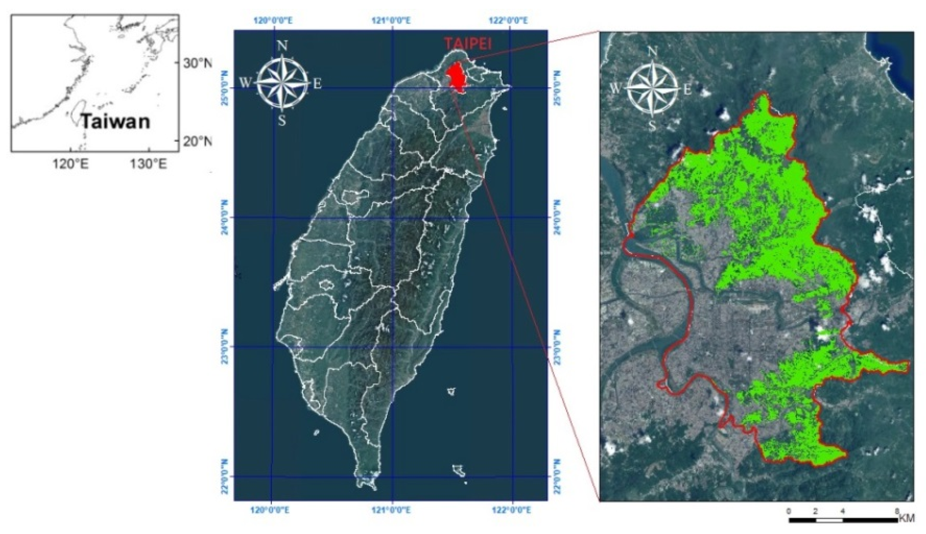
Figure 1.
Location of the research area in Taipei, Taiwan.
Figure 1.
Location of the research area in Taipei, Taiwan.
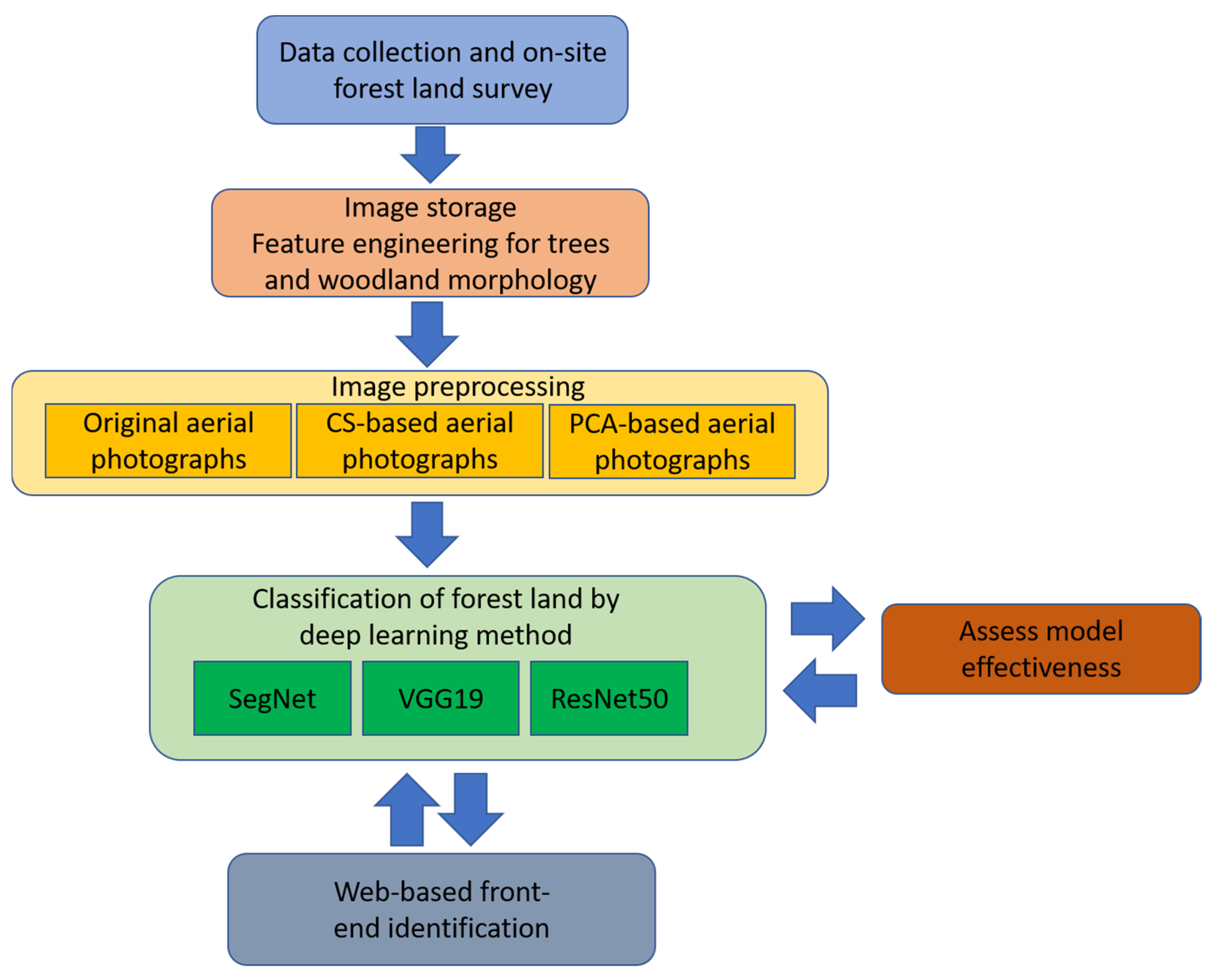
Figure 2.
Flowchart representing the methodology used for forest and vegetation type identification.
Figure 2.
Flowchart representing the methodology used for forest and vegetation type identification.
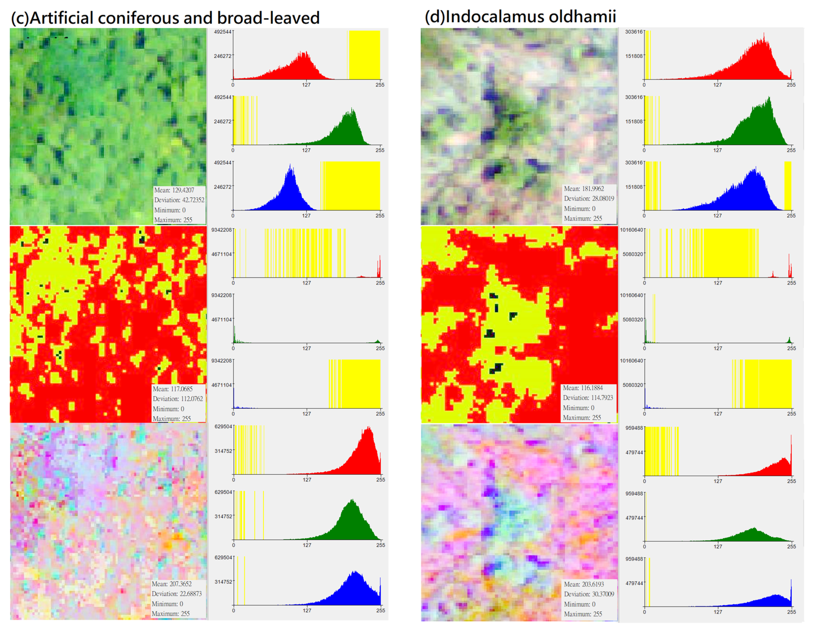
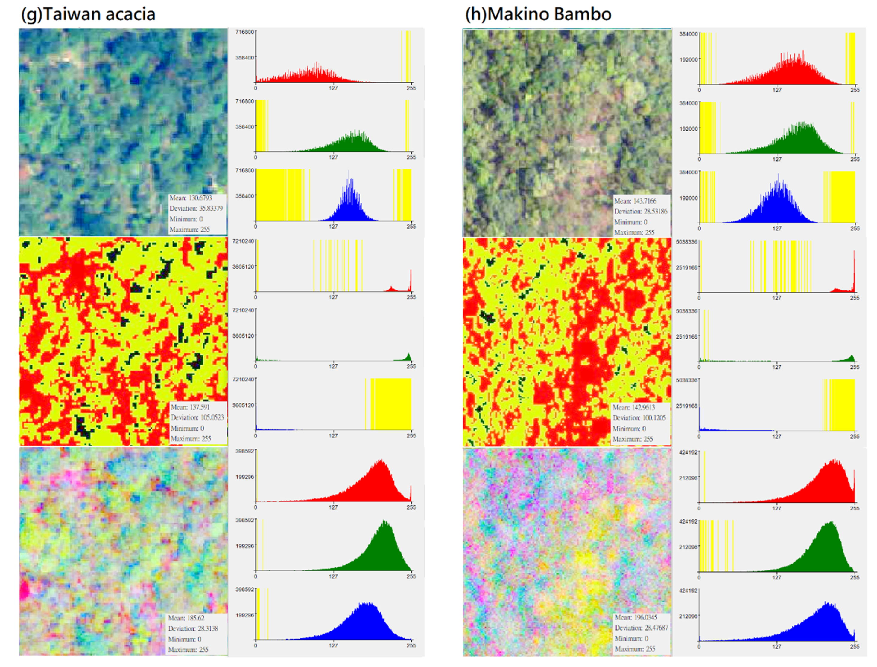
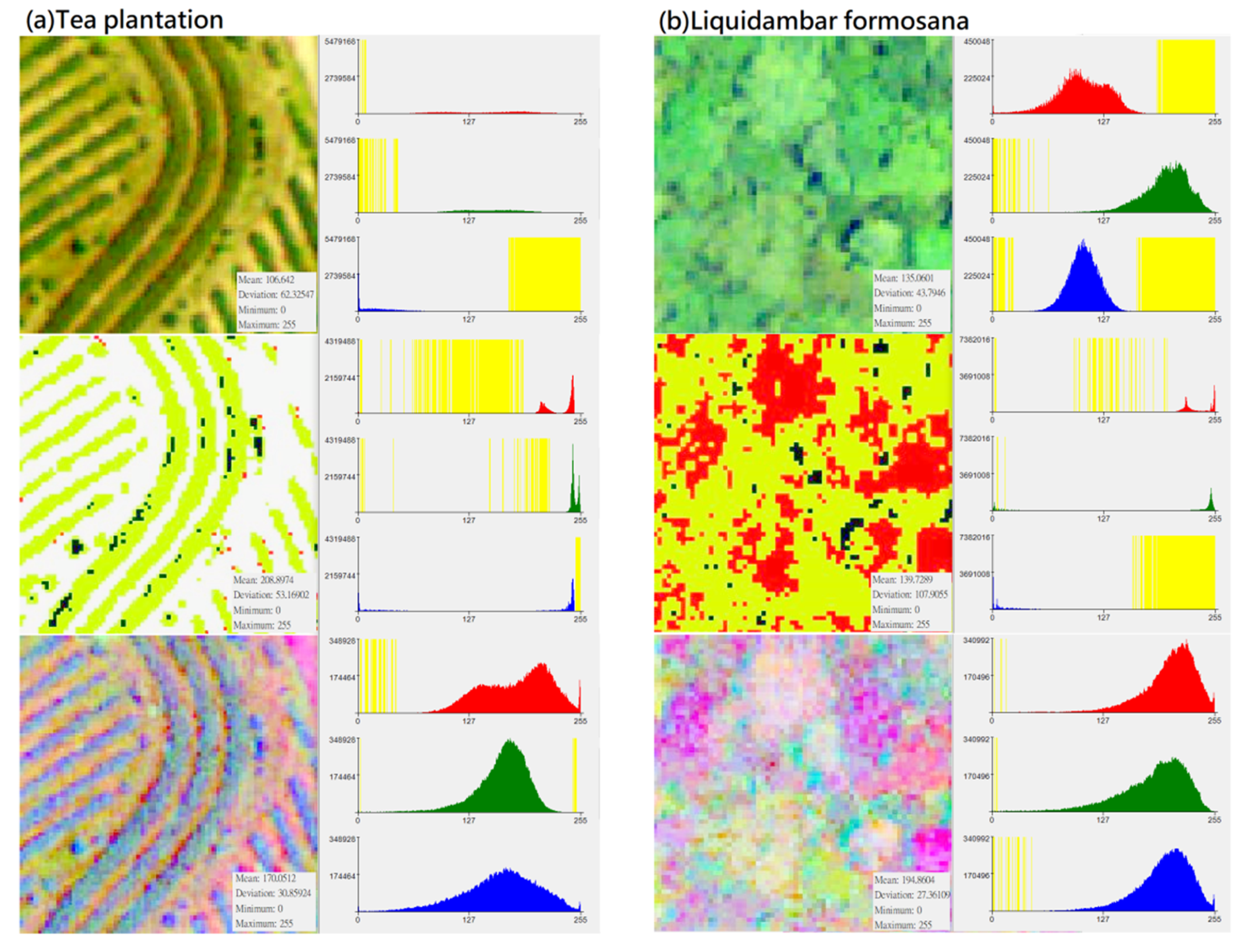
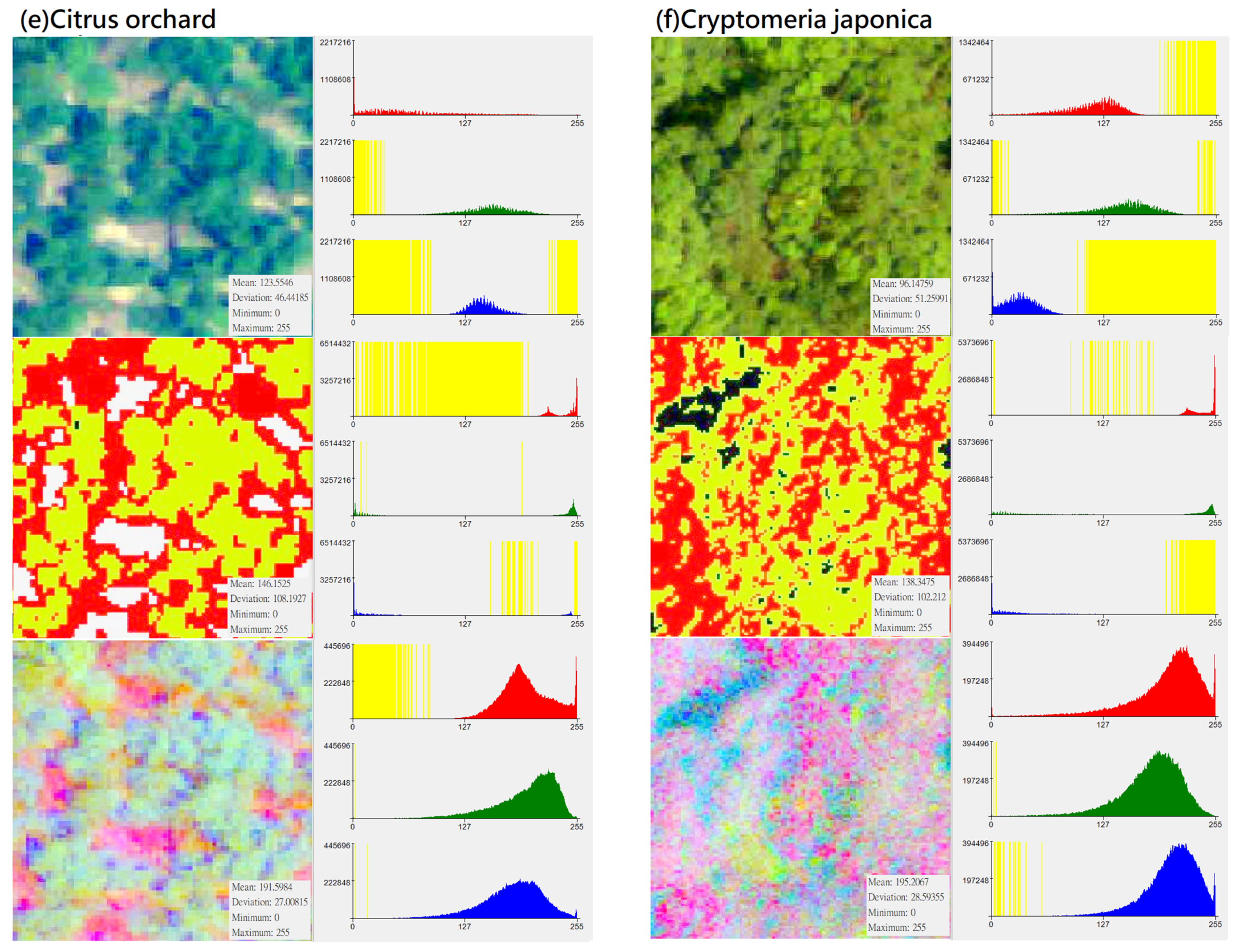
Figure 3.
Distribution of DN value (X-axis) and pixel number (Y-axis) of different vegetation types in “original photographs”, “CS-based aerial photographs“, “PCA-based aerial photographs“ (yellow represents the zero value area, subfigures (a–h) represent several types of forest and vegetation types that this research mainly wants to identify).
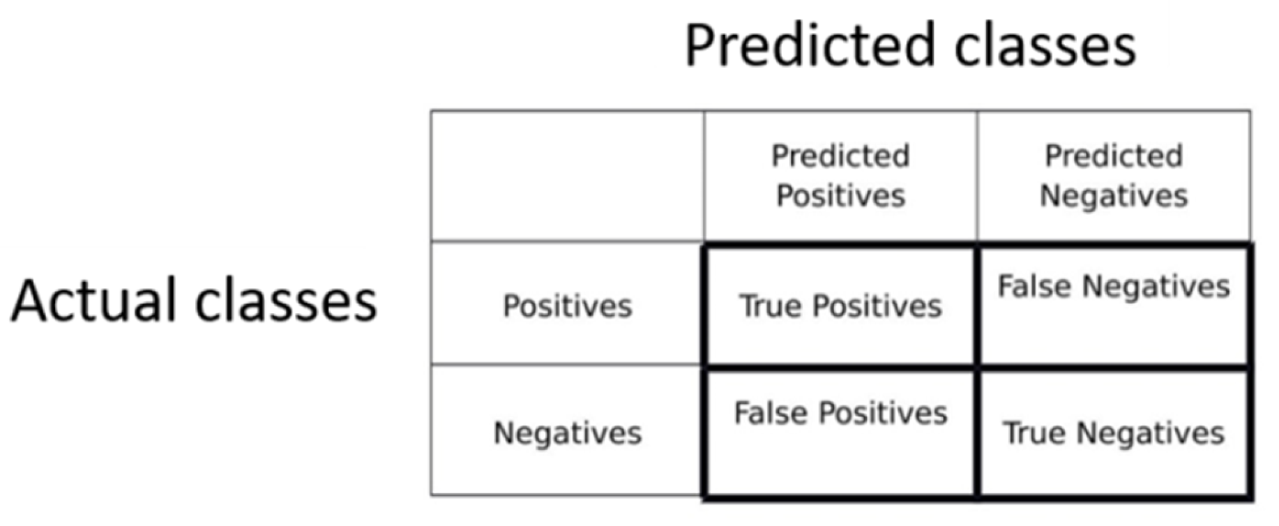
Figure 4.
Confusion matrix.
Figure 4.
Confusion matrix.
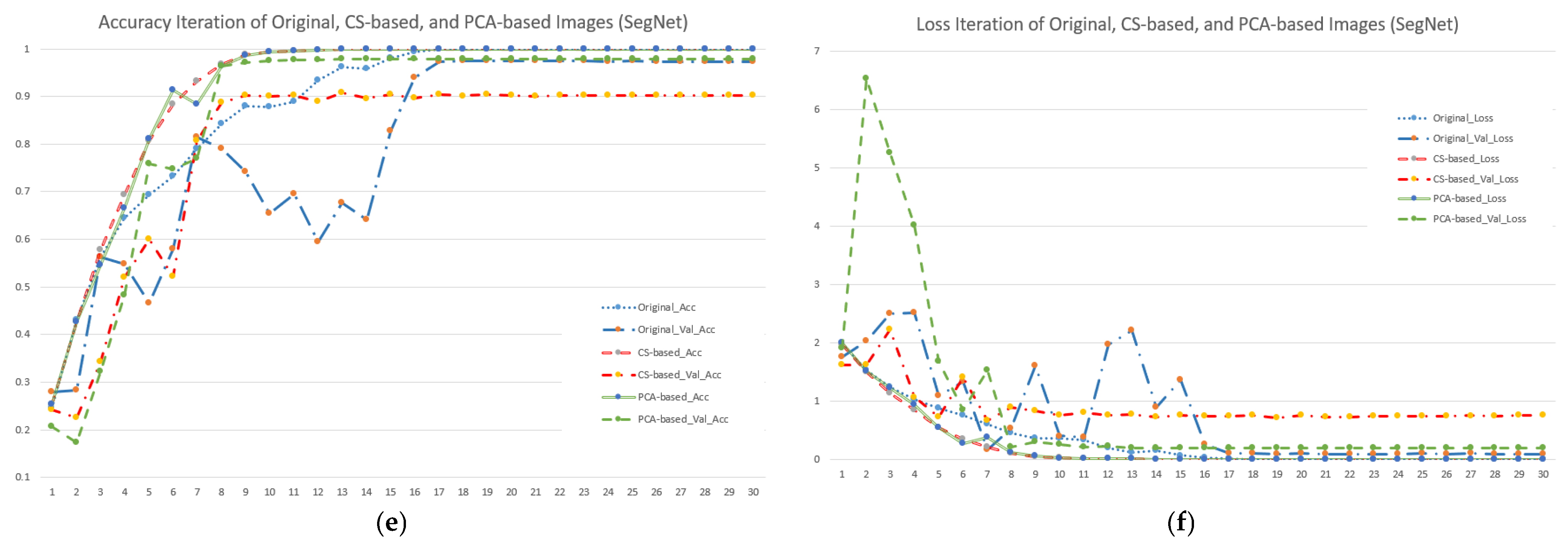
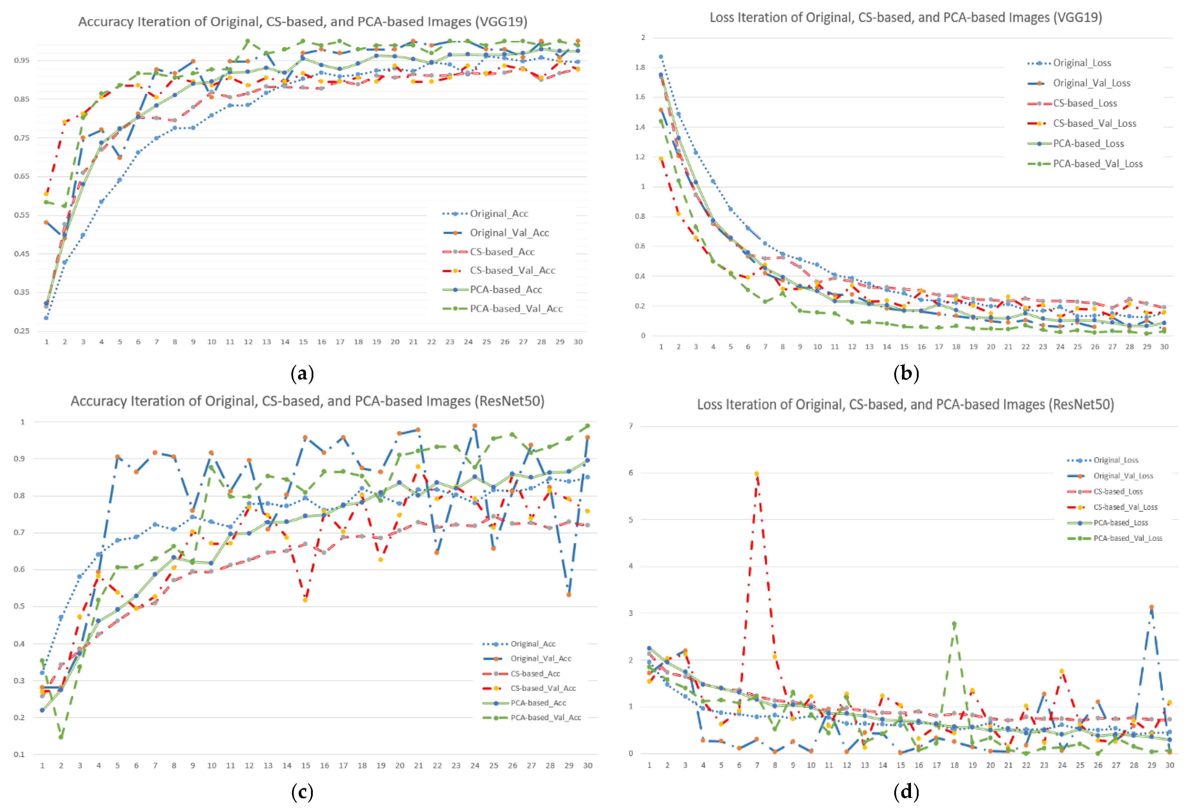
Figure 5.
Accuracy and loss iterations of different image and model combinations when using seven forest and vegetation types (subfigures (a,c,e) represent accuracy iterations of VGG19, ResNet50 and SegNet; subfigures (b,d,f) represent loss iterations of VGG19, ResNet50 and SegNet).
Figure 5.
Accuracy and loss iterations of different image and model combinations when using seven forest and vegetation types (subfigures (a,c,e) represent accuracy iterations of VGG19, ResNet50 and SegNet; subfigures (b,d,f) represent loss iterations of VGG19, ResNet50 and SegNet).
Figure 6.
Proposed user interface for uploading images.
Figure 6.
Proposed user interface for uploading images.
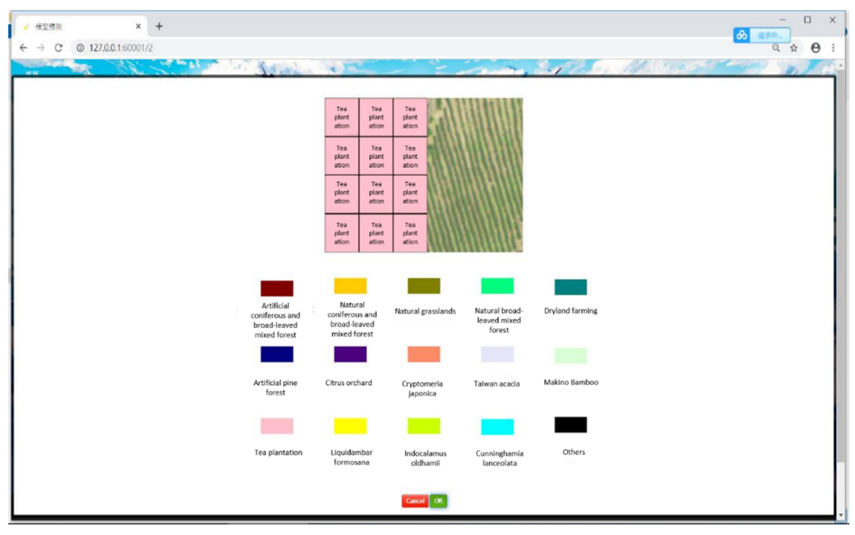
Figure 7.
Representation of returned results in a browser.
Figure 7.
Representation of returned results in a browser.
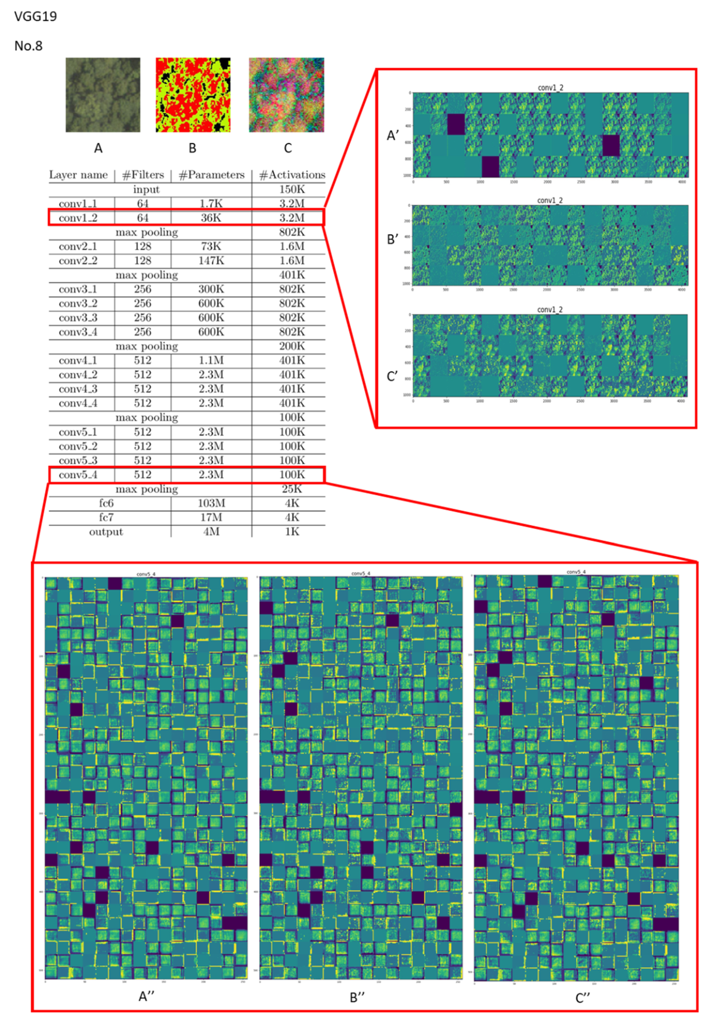
Figure 8.
Visualization of feature channels for three different kinds of input in the last layer of the “conv1” and “conv5” stages in VGG19 (vegetation type: Cryptomeria Japonica (Type 8)).
Figure 8.
Visualization of feature channels for three different kinds of input in the last layer of the “conv1” and “conv5” stages in VGG19 (vegetation type: Cryptomeria Japonica (Type 8)).
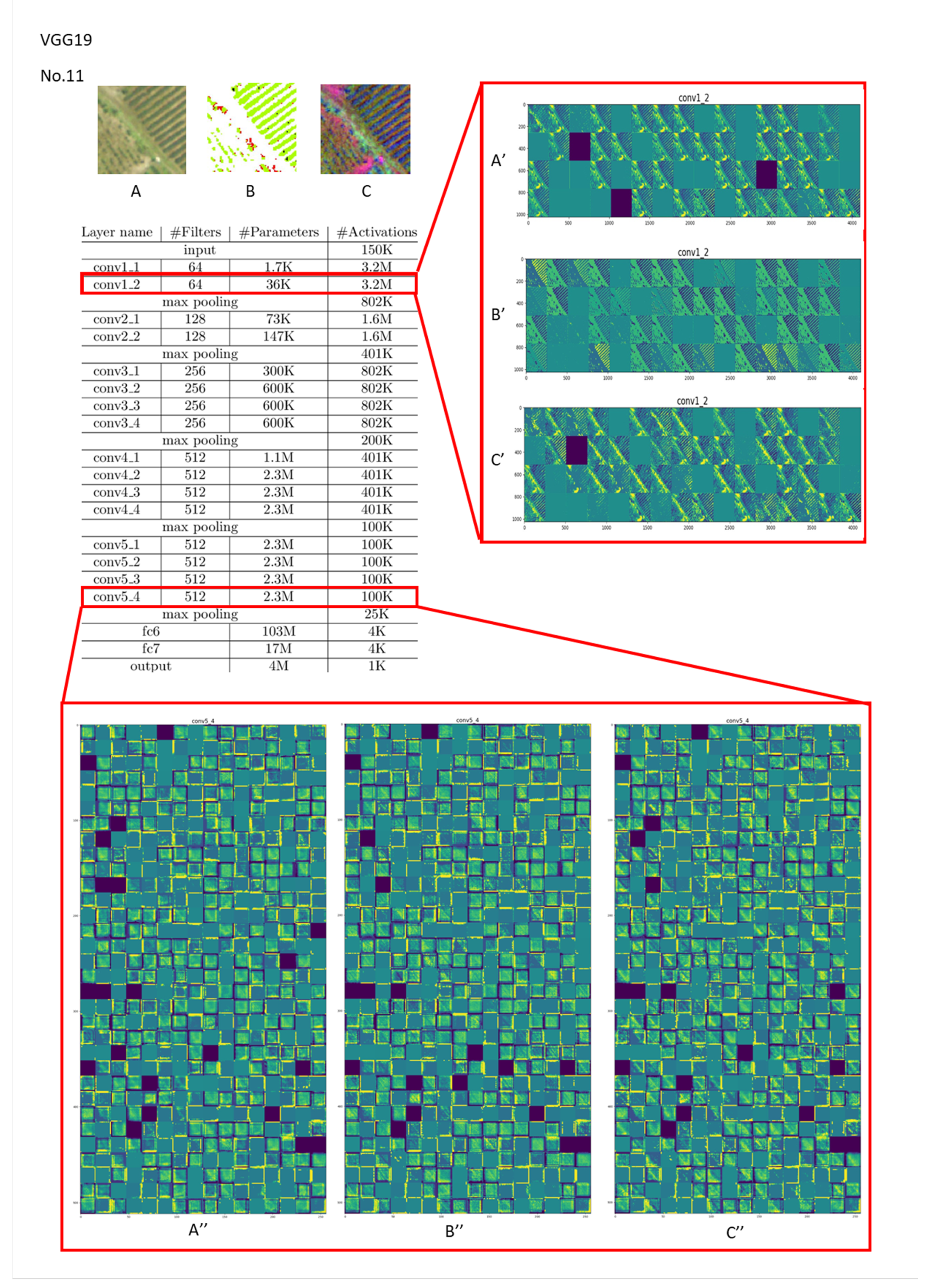
Figure 9.
Visualization of feature channels for three different kinds of input in the last layer of the “conv1” and “conv5” stages in VGG19 (vegetation type: tea plantation (Type 11)).
Figure 9.
Visualization of feature channels for three different kinds of input in the last layer of the “conv1” and “conv5” stages in VGG19 (vegetation type: tea plantation (Type 11)).
Table 1.
Fourteen types of forest and vegetation.
Table 2.
The versions of Python libraries used in this research.
Table 2.
The versions of Python libraries used in this research.
| Python Library | Version |
|---|
| TensorFlow-gpu | 2.0.0-rc0 |
| Keras | 2.3.1 |
| Numpy | 1.18.1 |
| Matplotlib | 3.1.3 |
| sklearn | 0.22.1 |
| pandas | 1.0.3 |
Table 3.
Model parameter sizes used in this research.
Table 3.
Model parameter sizes used in this research.
| | VGG19 (Model: “Sequential”) | ResNet50 | SegNet |
|---|
| Total params | 20.024.384 | 23.561.152 | 31.821.646 |
| Trainable params | 20.024.384 | 23.508.032 | 31.804.750 |
| Non-trainable params | 0 | 53.120 | 16.896 |
Table 4.
Precision, recall, and F1 score of original aerial photography when using VGG19, ResNet50, and SegNet in 14 types of images (ID number: (1) Artificial coniferous and broad-leaved mixed forest, (2) Natural coniferous and broad-leaved mixed forest, (3) Natural grasslands, (4) Natural broad-leaved mixed forest, (5) Dryland farming, (6) Artificial pine forest, (7) Citrus orchard, (8) Cryptomeria japonica, (9) Taiwan acacia, (10) Makino Bamboo, (11) Tea plantation, (12) Liquidambar formosana, (13) Indocalamus oldhamii, and (14) Cunninghamia lanceolata).
| Forest and Vegetation Types (Original Photographs) |
|---|
| | VGG19 (Accuracy: 93%) | ResNet50 (Accuracy: 66.00%) | SegNet (Accuracy: 82.00%) |
|---|
| ID | Precision | Recall | F1 | Precision | Recall | F1 | Precision | Recall | F1 |
|---|
| 1 | 1.00 | 0.98 | 0.99 | 0.45 | 0.86 | 0.59 | 0.67 | 1.00 | 0.80 |
| 2 | 0.90 | 0.90 | 0.90 | 1.00 | 0.65 | 0.79 | 1.00 | 0.75 | 0.86 |
| 3 | 1.00 | 1.00 | 1.00 | 0.00 | 0.00 | 0.00 | 1.00 | 1.00 | 1.00 |
| 4 | 1.00 | 1.00 | 1.00 | 1.00 | 0.84 | 0.91 | 0.89 | 1.00 | 0.94 |
| 5 | 0.69 | 1.00 | 0.81 | 0.27 | 0.71 | 0.40 | 1.00 | 0.89 | 0.94 |
| 6 | 1.00 | 1.00 | 1.00 | 0.00 | 0.00 | 0.00 | 0.59 | 0.96 | 0.73 |
| 7 | 0.71 | 0.89 | 0.79 | 0.40 | 1.00 | 0.57 | 0.00 | 0.00 | 0.00 |
| 8 | 0.84 | 0.95 | 0.89 | 0.94 | 1.00 | 0.97 | 1.00 | 1.00 | 1.00 |
| 9 | 0.95 | 0.69 | 0.80 | 0.88 | 0.53 | 0.66 | 1.00 | 1.00 | 1.00 |
| 10 | 1.00 | 1.00 | 1.00 | 0.64 | 1.00 | 0.78 | 0.63 | 1.00 | 0.77 |
| 11 | 1.00 | 1.00 | 1.00 | 0.88 | 1.00 | 0.94 | 1.00 | 0.62 | 0.76 |
| 12 | 1.00 | 1.00 | 1.00 | 0.82 | 1.00 | 0.90 | 1.00 | 0.31 | 0.48 |
| 13 | 1.00 | 1.00 | 1.00 | 0.44 | 0.50 | 0.47 | 0.95 | 0.43 | 0.59 |
| 14 | 0.95 | 0.81 | 0.88 | 1.00 | 0.84 | 0.91 | 0.85 | 0.66 | 0.74 |
Table 5.
Precision, recall, and F1 score of original aerial photography when using VGG19, ResNet50, and SegNet.
Table 5.
Precision, recall, and F1 score of original aerial photography when using VGG19, ResNet50, and SegNet.
Seven Forest and Vegetation Types (Type 1, Type 2, Type 4, Type 7, Type 8, Type 10, and Type 11)
(Original Photographs) |
|---|
| | VGG19 (Accuracy: 98%) | ResNet50 (Accuracy: 81%) | SegNet (Accuracy: 95.65%) |
|---|
| ID | Precision | Recall | F1 | Precision | Recall | F1 | Precision | Recall | F1 |
|---|
| 1 | 0.98 | 1.00 | 0.99 | 0.88 | 0.26 | 0.40 | 0.85 | 1.00 | 0.92 |
| 2 | 1.00 | 0.89 | 0.94 | 1.00 | 1.00 | 1.00 | 1.00 | 1.00 | 1.00 |
| 4 | 1.00 | 1.00 | 1.00 | 0.57 | 1.00 | 0.73 | 1.00 | 1.00 | 1.00 |
| 7 | 0.90 | 1.00 | 0.95 | 0.66 | 1.00 | 0.79 | 1.00 | 0.40 | 0.40 |
| 8 | 1.00 | 0.93 | 0.97 | 1.00 | 0.96 | 0.98 | 1.00 | 1.00 | 1.00 |
| 10 | 0.80 | 1.00 | 0.89 | 1.00 | 1.00 | 1.00 | 1.00 | 1.00 | 1.00 |
| 11 | 1.00 | 1.00 | 1.00 | 1.00 | 1.00 | 1.00 | 1.00 | 0.99 | 0.99 |
Table 6.
Precision, recall, and F1 score of original aerial photography when using VGG19, ResNet50, and SegNet.
Table 6.
Precision, recall, and F1 score of original aerial photography when using VGG19, ResNet50, and SegNet.
| Fourteen Forest and Vegetation Types |
|---|
| Algorithm | Training Time (30 Epochs) | Testing Time (500 Photographs) | Accuracy |
|---|
| VGG19 | 275.84 s | 5.48 s | 0.93 |
| ResNet50 | 778 s | 44 s | 0.66 |
| SegNet | 1540 s | 57 s | 0.82 |
| Seven Forest and Vegetation Types (Type 1, Type 2, Type 4, Type 7, Type 8, Type 10, and Type 11) |
| Algorithm | Training Time (30 Epochs) | Testing Time (231 Photographs) | Accuracy |
| VGG19 | 121.56 s | 2.73 s | 0.98 |
| ResNet50 | 378 s | 40 s | 0.81 |
| SegNet | 681 s | 26 s | 0.95 |
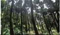
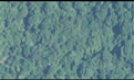
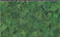
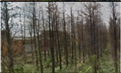
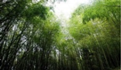
Table 7.
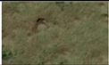
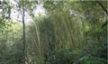
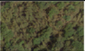
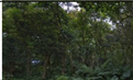
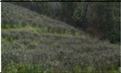
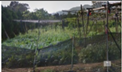
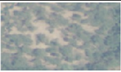
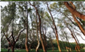
Fourteen types (original aerial photograph and CS-based photographs) (ID number: (1) Artificial coniferous and broad-leaved mixed forest, (2) Natural coniferous and broad-leaved mixed forest, (3) Natural grasslands, (4) Natural broad-leaved mixed forest, (5) Dryland farming, (6) Artificial pine forest, (7) Citrus orchard, (8) Cryptomeria japonica, (9) Taiwan acacia, (10) Makino Bamboo, (11) Tea plantation, (12) Liquidambar formosana, (13) Indocalamus oldhamii, and (14) Cunninghamia lanceolata).
Table 7.
Fourteen types (original aerial photograph and CS-based photographs) (ID number: (1) Artificial coniferous and broad-leaved mixed forest, (2) Natural coniferous and broad-leaved mixed forest, (3) Natural grasslands, (4) Natural broad-leaved mixed forest, (5) Dryland farming, (6) Artificial pine forest, (7) Citrus orchard, (8) Cryptomeria japonica, (9) Taiwan acacia, (10) Makino Bamboo, (11) Tea plantation, (12) Liquidambar formosana, (13) Indocalamus oldhamii, and (14) Cunninghamia lanceolata).
| Forest and Vegetation Types | Original Aerial Photograph | CS-Based Aerial
Photograph | Forest and Vegetation Types | Original Aerial Photograph | CS-Based Aerial
Photograph |
|---|
| (1) | ![Remotesensing 13 04036 i029]() | ![Remotesensing 13 04036 i030]() | (8) | ![Remotesensing 13 04036 i031]() | ![Remotesensing 13 04036 i032]() |
| (2) | ![Remotesensing 13 04036 i033]() | ![Remotesensing 13 04036 i034]() | (9) | ![Remotesensing 13 04036 i035]() | ![Remotesensing 13 04036 i036]() |
| (3) | ![Remotesensing 13 04036 i037]() | ![Remotesensing 13 04036 i038]() | (10) | ![Remotesensing 13 04036 i039]() | ![Remotesensing 13 04036 i040]() |
| (4) | ![Remotesensing 13 04036 i041]() | ![Remotesensing 13 04036 i042]() | (11) | ![Remotesensing 13 04036 i043]() | ![Remotesensing 13 04036 i044]() |
| (5) | ![Remotesensing 13 04036 i045]() | ![Remotesensing 13 04036 i046]() | (12) | ![Remotesensing 13 04036 i047]() | ![Remotesensing 13 04036 i048]() |
| (6) | ![Remotesensing 13 04036 i049]() | ![Remotesensing 13 04036 i050]() | (13) | ![Remotesensing 13 04036 i051]() | ![Remotesensing 13 04036 i052]() |
| (7) | ![Remotesensing 13 04036 i053]() | ![Remotesensing 13 04036 i054]() | (14) | ![Remotesensing 13 04036 i055]() | ![Remotesensing 13 04036 i056]() |
Table 8.
Precision, recall, and F1 score of CS-based photographs when using VGG19, ResNet50, and SegNet.
Table 8.
Precision, recall, and F1 score of CS-based photographs when using VGG19, ResNet50, and SegNet.
| Seven Forest and Vegetation Types (CS-Based Photographs) |
|---|
| | VGG19 (Accuracy: 95%) | Resnet50 (Accuracy: 60%) | Segnet (Accuracy: 95.69%) |
|---|
| | Precision | Recall | F1 | Precision | Recall | F1 | Precision | Recall | F1 |
|---|
| 1 | 1.00 | 0.98 | 0.99 | 0.32 | 0.39 | 0.35 | 0.88 | 1.00 | 0.94 |
| 2 | 1.00 | 1.00 | 1.00 | 1.00 | 0.80 | 0.89 | 1.00 | 0.82 | 0.90 |
| 4 | 1.00 | 1.00 | 1.00 | 0.43 | 0.94 | 0.59 | 1.00 | 1.00 | 1.00 |
| 7 | 1.00 | 1.00 | 1.00 | 1.00 | 1.00 | 1.00 | 0.87 | 0.87 | 0.87 |
| 8 | 0.81 | 0.98 | 0.89 | 0.94 | 0.30 | 0.45 | 1.00 | 0.91 | 0.96 |
| 10 | 0.88 | 0.41 | 0.56 | 0.00 | 0.00 | 0.00 | 1.00 | 0.87 | 0.93 |
| 11 | 1.00 | 1.00 | 1.00 | 1.00 | 1.00 | 1.00 | 1.00 | 1.00 | 1.00 |
Table 9.
Precision, recall, and F1 score of original aerial photography when using VGG19, ResNet50, and SegNet for 14 types of images (CS-based photographs).
Table 9.
Precision, recall, and F1 score of original aerial photography when using VGG19, ResNet50, and SegNet for 14 types of images (CS-based photographs).
| CS-Based Photographs (14 Forest and Vegetation Types) |
|---|
| | VGG19 (Accuracy: 93%) | Resnet50 (Accuracy: 32%) | Segnet (Accuracy: 87.20%) |
|---|
| | Precision | Recall | F1 | Precision | Recall | F1 | Precision | Recall | F1 |
|---|
| 1 | 0.89 | 0.86 | 0.88 | 0.00 | 0.00 | 0.00 | 0.82 | 1.00 | 0.90 |
| 2 | 1.00 | 1.00 | 1.00 | 0.43 | 1.00 | 0.60 | 1.00 | 0.88 | 0.94 |
| 3 | 0.92 | 0.94 | 0.93 | 0.19 | 0.44 | 0.27 | 1.00 | 0.12 | 0.22 |
| 4 | 0.87 | 1.00 | 0.93 | 0.14 | 0.91 | 0.25 | 0.88 | 1.00 | 0.93 |
| 5 | 0.86 | 1.00 | 0.92 | 0.83 | 0.54 | 0.66 | 0.88 | 0.82 | 0.85 |
| 6 | 0.88 | 0.92 | 0.90 | 0.00 | 0.00 | 0.00 | 1.00 | 0.93 | 0.96 |
| 7 | 1.00 | 1.00 | 1.00 | 1.00 | 0.53 | 0.70 | 0.28 | 1.00 | 0.44 |
| 8 | 0.86 | 0.91 | 0.89 | 0.00 | 0.00 | 0.00 | 0.96 | 0.93 | 0.95 |
| 9 | 1.00 | 0.91 | 0.95 | 1.00 | 0.08 | 0.14 | 0.89 | 0.91 | 0.90 |
| 10 | 0.75 | 0.71 | 0.73 | 0.00 | 0.00 | 0.00 | 1.00 | 0.84 | 0.91 |
| 11 | 1.00 | 1.00 | 1.00 | 0.95 | 1.00 | 0.98 | 1.00 | 0.92 | 0.96 |
| 12 | 1.00 | 0.96 | 0.98 | 0.00 | 0.00 | 0.00 | 1.00 | 1.00 | 1.00 |
| 13 | 1.00 | 0.93 | 0.97 | 0.54 | 0.82 | 0.65 | 1.00 | 0.90 | 0.95 |
| 14 | 1.00 | 0.87 | 0.93 | 0.67 | 0.05 | 0.09 | 0.98 | 1.00 | 0.99 |
Table 10.
Computational time and accuracy for feature-based images when using VGG19, ResNet50, and SegNet.
Table 10.
Computational time and accuracy for feature-based images when using VGG19, ResNet50, and SegNet.
| Fourteen Forest and Vegetation Types |
|---|
| Algorithm | Training Time (30 Epochs) | Testing Time (500 Images) | Accuracy |
|---|
| VGG19 | 285.52 s | 5.71 s | 0.93 |
| ResNet50 | 777 s | 44 s | 0.32 |
| SegNet | 1488 s | 57 s | 0.87 |
| Seven Forest and Vegetation Types |
| Algorithm | Training Time (30 Epochs) | Testing Time (231 Images) | Accuracy |
| VGG19 | 127.61 s | 2.89 s | 0.95 |
| ResNet50 | 371 s | 40 s | 0.60 |
| SegNet | 711 s | 19 s | 0.96 |
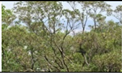
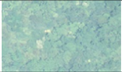
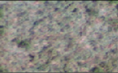
Table 11.
Fourteen forest and vegetation types (original aerial photograph and PCA-based photograph) (ID number: (1) Artificial coniferous and broad-leaved mixed forest, (2) Natural coniferous and broad-leaved mixed forest, (3) Natural grasslands, (4) Natural broad-leaved mixed forest, (5) Dryland farming, (6) Artificial pine forest, (7) Citrus orchard, (8) Cryptomeria japonica, (9) Taiwan acacia, (10) Makino Bamboo, (11) Tea plantation, (12) Liquidambar formosana, (13) Indocalamus oldhamii, and (14) Cunninghamia lanceolata).
| Forest and Vegetation Types | Original Aerial
Photograph | PCA-Based Aerial
Photograph | Forest and Vegetation Types | Original Aerial Photograph | PCA-Based Aerial Photograph |
|---|
| (1) | ![Remotesensing 13 04036 i057]() | ![Remotesensing 13 04036 i058]() | (8) | ![Remotesensing 13 04036 i059]() | ![Remotesensing 13 04036 i060]() |
| (2) | ![Remotesensing 13 04036 i061]() | ![Remotesensing 13 04036 i062]() | (9) | ![Remotesensing 13 04036 i063]() | ![Remotesensing 13 04036 i064]() |
| (3) | ![Remotesensing 13 04036 i065]() | ![Remotesensing 13 04036 i066]() | (10) | ![Remotesensing 13 04036 i067]() | ![Remotesensing 13 04036 i068]() |
| (4) | ![Remotesensing 13 04036 i069]() | ![Remotesensing 13 04036 i070]() | (11) | ![Remotesensing 13 04036 i071]() | ![Remotesensing 13 04036 i072]() |
| (5) | ![Remotesensing 13 04036 i073]() | ![Remotesensing 13 04036 i074]() | (12) | ![Remotesensing 13 04036 i075]() | ![Remotesensing 13 04036 i076]() |
| (6) | ![Remotesensing 13 04036 i077]() | ![Remotesensing 13 04036 i078]() | (13) | ![Remotesensing 13 04036 i079]() | ![Remotesensing 13 04036 i080]() |
| (7) | ![Remotesensing 13 04036 i081]() | ![Remotesensing 13 04036 i082]() | (14) | ![Remotesensing 13 04036 i083]() | ![Remotesensing 13 04036 i084]() |
Table 12.
Precision, recall, and F1 score of original aerial photography when using VGG19, ResNet50, and SegNet in 14 types of images (PCA-based photographs).
Table 12.
Precision, recall, and F1 score of original aerial photography when using VGG19, ResNet50, and SegNet in 14 types of images (PCA-based photographs).
| Fourteen PCA-Based Photographs |
|---|
| | VGG19 (Accuracy: 96%) | ResNet50 (Accuracy: 93%) | SegNet (Accuracy: 98.20%) |
|---|
| | Precision | Recall | F1 | Precision | Recall | F1 | Precision | Recall | F1 |
|---|
| 1 | 0.93 | 1.00 | 0.96 | 1.00 | 0.75 | 0.85 | 0.97 | 1.00 | 0.98 |
| 2 | 1.00 | 1.00 | 1.00 | 1.00 | 1.00 | 1.00 | 1.00 | 1.00 | 1.00 |
| 3 | 1.00 | 0.86 | 0.93 | 0.98 | 1.00 | 0.99 | 1.00 | 0.97 | 0.98 |
| 4 | 1.00 | 1.00 | 1.00 | 0.95 | 1.00 | 0.97 | 0.93 | 1.00 | 0.96 |
| 5 | 1.00 | 1.00 | 1.00 | 0.88 | 1.00 | 0.94 | 0.95 | 0.91 | 0.93 |
| 6 | 0.75 | 1.00 | 0.86 | 1.00 | 1.00 | 1.00 | 1.00 | 0.98 | 0.99 |
| 7 | 0.93 | 1.00 | 0.96 | 1.00 | 1.00 | 1.00 | 0.92 | 1.00 | 0.96 |
| 8 | 0.98 | 0.85 | 0.91 | 0.98 | 0.91 | 0.95 | 0.98 | 1.00 | 0.99 |
| 9 | 1.00 | 1.00 | 1.00 | 0.96 | 0.89 | 0.92 | 1.00 | 1.00 | 1.00 |
| 10 | 0.91 | 0.83 | 0.87 | 1.00 | 0.58 | 0.74 | 1.00 | 1.00 | 1.00 |
| 11 | 1.00 | 1.00 | 1.00 | 1.00 | 0.97 | 0.98 | 1.00 | 1.00 | 1.00 |
| 12 | 1.00 | 1.00 | 1.00 | 0.74 | 1.00 | 0.85 | 1.00 | 1.00 | 1.00 |
| 13 | 1.00 | 0.95 | 0.97 | 1.00 | 0.95 | 0.98 | 1.00 | 0.91 | 0.96 |
| 14 | 0.93 | 0.98 | 0.96 | 0.79 | 1.00 | 0.88 | 0.97 | 0.98 | 0.98 |
Table 13.
Precision, recall, and F1 score of PCA-based images when using VGG19, ResNet50, and SegNet for seven forest and vegetation types (PCA-based photographs).
Table 13.
Precision, recall, and F1 score of PCA-based images when using VGG19, ResNet50, and SegNet for seven forest and vegetation types (PCA-based photographs).
| | VGG19 (Accuracy: 92%) | ResNet50 (Accuracy: 96%) | SegNet (Accuracy: 100%) |
|---|
| | Precision | Recall | F1 | Precision | Recall | F1 | Precision | Recall | F1 |
|---|
| 1 | 1.00 | 1.00 | 1.00 | 1.00 | 0.93 | 0.96 | 1.00 | 1.00 | 1.00 |
| 2 | 1.00 | 1.00 | 1.00 | 0.92 | 1.00 | 0.96 | 1.00 | 1.00 | 1.00 |
| 4 | 1.00 | 1.00 | 1.00 | 0.98 | 1.00 | 0.99 | 1.00 | 1.00 | 1.00 |
| 7 | 1.00 | 1.00 | 1.00 | 1.00 | 1.00 | 1.00 | 1.00 | 1.00 | 1.00 |
| 8 | 1.00 | 0.60 | 0.75 | 1.00 | 0.89 | 0.94 | 1.00 | 1.00 | 1.00 |
| 10 | 0.39 | 1.00 | 0.56 | 0.71 | 1.00 | 0.83 | 1.00 | 1.00 | 1.00 |
| 11 | 1.00 | 1.00 | 1.00 | 0.94 | 1.00 | 0.97 | 1.00 | 1.00 | 1.00 |
Table 14.
Computational time and accuracy for PCA-based images when using VGG19, ResNet50, and SegNet.
Table 14.
Computational time and accuracy for PCA-based images when using VGG19, ResNet50, and SegNet.
| Fourteen Forest and Vegetation Types |
|---|
| Algorithm | Training Time (30 Epochs) | Testing Time (500 Images) | Accuracy |
|---|
| VGG19 | 280.91 s | 5.58 s | 0.96 |
| ResNet50 | 778 s | 44 s | 0.93 |
| SegNet | 1497 s | 57 s | 0.98 |
| Seven Forest and Vegetation Types |
| Algorithm | Training Time (30 Epochs) | Testing Time (500 Images) | Accuracy |
| VGG19 | 130.17 s | 2.64 s | 0.92 |
| ResNet50 | 367 s | 40 s | 0.96 |
| SegNet | 670 s | 19 s | 1.00 |


