Effects of Variable Eruption Source Parameters on Volcanic Plume Transport: Example of the 23 November 2013 Paroxysm of Etna

Abstract

The purpose of the present paper is to investigate the effects of variable eruption source parameters on volcanic plume transport in the Mediterranean basin after the paroxysm of Mount Etna on 23 November 2013. This paroxysm was characterized by a north-east transport of ash and gas, caused by a low-pressure system in northern Italy. It is evaluated here in a joint approach considering the WRF-Chem model configured with eruption source parameters (ESPs) obtained elaborating the raw data from the VOLDORAD-2B (V2B) Doppler radar system. This allows the inclusion of the transient and fluctuating nature of the volcanic emissions to accurately model the atmospheric dispersion of ash and gas. Two model configurations were considered: the first with the climax values for the ESP and the second with the time-varying ESP according to the time profiles of the mass eruption rate recorded by the V2B radar. It is demonstrated that the second configuration produces a considerably better comparison with satellite retrievals from different sensors platforms (Ozone Mapping and Profiler Suite, Meteosat Second-Generation Spinning Enhanced Visible and Infrared Imager, and Visible Infrared Imaging Radiometer Suite). In the context of volcanic ash transport dispersion modeling, our results indicate the need for (i) the use of time-varying ESP, and (ii) a joint approach between an online coupled chemical transport model like WRF-Chem and direct near-source measurements, such as those carried out by the V2B Doppler radar system.

1. Introduction

Explosive volcanic eruptions inject large amounts of particles, aerosols, and gases into the atmosphere, where they are carried away for several thousand kilometers and remain suspended in the air for several days or months. Once in the atmosphere, these ash particles, typically ranging from a few millimeters to a few micrometers, are usually involved in physico-chemical processes, influencing weather and climate [1]. While the transport of ash particles mainly concerns airport security and flight safety and the sedimentation of ash particles affects ground infrastructures and human health, the oxidation of the volcanogenic SO₂ leads to the formation of sulfate particles, through chemical and microphysical processes [2]. Sulfate particles can reduce the incoming shortwave radiation by increasing the scattering of sunlight in the atmosphere [1].

From the point of view of airport and flight security, it should be pointed out that the critical region affected by an explosive eruption may be of the order of 10³ km or more within 24 h after the onset of ash-producing eruptions [3]. In this context, the provision of a reliable forecast of the volcanic aerosols dispersion, ash fallout, and interactions with local meteorology requires the utilization of modern chemical transport models (CTMs). Although of crucial importance, this is quite a challenging task because of large uncertainties in CTM basically with respect to the definitions of the eruption source parameters (ESPs, e.g., mass eruption rate (MER), plume height, total grain-size distribution (TGSD), and eruption duration) and model parameterizations of internal processes like particle settling, optical properties, and aerosol feedback with radiation and microphysics [4,5]. It is also important to emphasize the need to consider the transient and fluctuating nature of the volcanic emissions to accurately model atmospheric dispersion of ash and gas. Special attention should be dedicated to specifying the injection height whatever technique is being used, namely Eulerian 1-D column models [6,7], idealized umbrella clouds profiles [8], constant profiles [9], or more complex parameterization derived from observations.

Mount Etna is an active volcano with a strong recent activity that has produced at least 11 explosive eruptions in the early months of 2021 [10], and more than 200 since 1979 [11]. If we consider the last century, the classification of Mount Etna’s explosive eruptions spans a broad range if expressed in terms of duration, mass eruption rates, and column height. In this context, two end-members can be considered, namely (i) the 5 January 1990, representative of a strong and short-lived sub-Plinian eruption, with 45 min climax, a column height up to 15 km above sea level (a.s.l.), and an average MER of 7 × 10⁶ kg s⁻¹ [12], and (ii) the weak and long-lived eruption of March 2002 that lasted almost two months, with a lower eruptive column (max 7 km a.s.l.) and an average MER of 5 × 10⁴ kg s⁻¹ [13].

The need for a ground-based radar system originates from the poor temporal coverage of the satellite sensors on various platforms that are generally used to track volcanic plumes, and from their limitations during overcast weather and early development of the eruptive column. Ground-based Doppler radars can monitor volcanic tephra emissions by probing atmospheric volumes near the emission source, providing direct measurements of tephra reflectivity and Doppler velocities at a high acquisition rate. In this context, a pulsed Doppler radar VOLDORAD-2B (V2B) has been dedicated to the continuous near-source monitoring of tephra emissions of Etna since 2009 by means of a fixed beam pointing to the summit craters from La Montagnola station 3 km south. With over 50 paroxysms recorded at Etna, it represents the first radar system fully integrated into a volcano instrumental network with the capacity to provide ejection velocities and MER in real-time [14,15,16]. Its 23.5 cm wavelength makes it sensitive to blocs, lapilli, and ash released during explosive eruptions, while signal attenuation by hydrometeors remains very limited.

The modern approach for the development of new-generation integrated meteorology (MetM) and chemical transport model (CTM) systems for the prediction of atmospheric composition and meteorology is based on the online and offline coupling strategy between the MetM and the CTM. It is important to highlight that the method of online integration modeling considering feedback mechanisms is more promising in the near future and could be beneficial for model improvements in both communities and the preliminary step toward the definition of fully integrated Earth-system models.

In this context, the use of volcanic ash transport and dispersion (VATD) models to estimate the concentration and the position of ash with time may be dated back to early 2000 [17]. They are usually based on an offline coupling between MetM models with a Lagrangian particle or Eulerian dispersion model. A Eulerian model FALL3D [18] coupled with the Weather Research and Forecast (WRF, [19,20]) model was utilized, for example, to study the transport of ash from the Cordon Caulle eruption in 2011 [21]. Among the Lagrangian particle trajectories models, we have utilized HYSPLIT [22], NAME [23], and Puff [24] in various contexts.

Likely, the Eyjafjallajökull eruption (15 April 2010) is the most studied recent event due to its strong impact on air traffic and economy in Europe. In this context, Plu et al. [25] simulated this eruption with the MOCAGE-CTM (Météo-France) and hourly changing MER from FPlume [6]. For the same eruption, Devenish et al. [26] and Webster et al. [27] both used the lagrangian model NAME while Folch et al. [28] used the FALL3D model. More recently, the CHIMERE model [29] coupled offline with WRF has been utilized to study the 18 March 2012 Mount Etna eruption [30].

The online coupling strategy is currently developed by using the WRF-Chem model [31,32,33] in which a specialized emission routine for the treatment of volcanic particles and gas (SO₂) has been implemented in its online chemistry-meteorology coupling framework [8]. This also permits inclusion of the direct and indirect feedback, together with other peculiar processes on the ash particles, like aggregation [33], microphysical nucleation [34], and the calculation of the optical properties (extinction coefficients and aerosol optical depth). Moreover, the “online CTM strategy” has been well suited for the utilization of time-dependent (transient) ESP like those from the V2B system. Nowadays, the WRF-Chem and radar combination, considering the transient and fluctuating nature of the volcanic emissions, represents an innovative advance to the current VATD modeling systems.

In this work, the source parameter evolution obtained from the measurements of the V2B Doppler radar system were assimilated inside the WRF-Chem input framework. The V2B raw data were pre-processed together with the other specific volcanic parameters to define a user-defined volcanic input file to allow multi-eruptions with a single run. The violent paroxysm of Mount Etna on 23 November 2013 was considered as a test case. Satellite retrievals by the Ozone Mapping and Profiler Suite (OMPS) sensor and the Visible Infrared Imaging Radiometer Suite (VIIRS) sensor both onboard the Suomi National Polar-orbiting Partnership (NPP) spacecraft, and the Meteosat Second Generation (MSG) Spinning Enhanced Visible and Infrared Imager (SEVIRI) images data were used to validate the outputs of the different setup configurations.

This work represents the preliminary step towards the forecast simulations of meteorology and ash dispersion of Mount Etna. This would be achievable in near real-time, assimilating into WRF-Chem model the input data from the VOLDORAD-2B monitoring system, aside from the end-member eruption scenarios used nowadays (one-weak long-lived emission similar to 2002–2003 and one strong short-lived eruption similar to 5 January 1990).

This new strategy (i.e., WRF-Chem and radar-based ESP) has three main objectives trying to respond to some of the new challenges of modern volcanology, namely (i) utilization of realistic time-dependent ESP and their assimilation in an online coupled CTM, (ii) provision of near-real time maps of volcanic aerosols that may help in identifying potential risk regions for flight security, and (iii) analysis of the effects of volcanic aerosols in atmospheric (longwave and shortwave) radiation.

The paper is organized as follows: Section 2 is dedicated to the description of the material and methods utilized in this work, in particular the suite of the remote sensing data and the configurations of the modeling system; in Section 3, we present all the simulations results and their comparison with experimental data; and in Section 4, we report the conclusions of the present study.

2. Materials and Methods

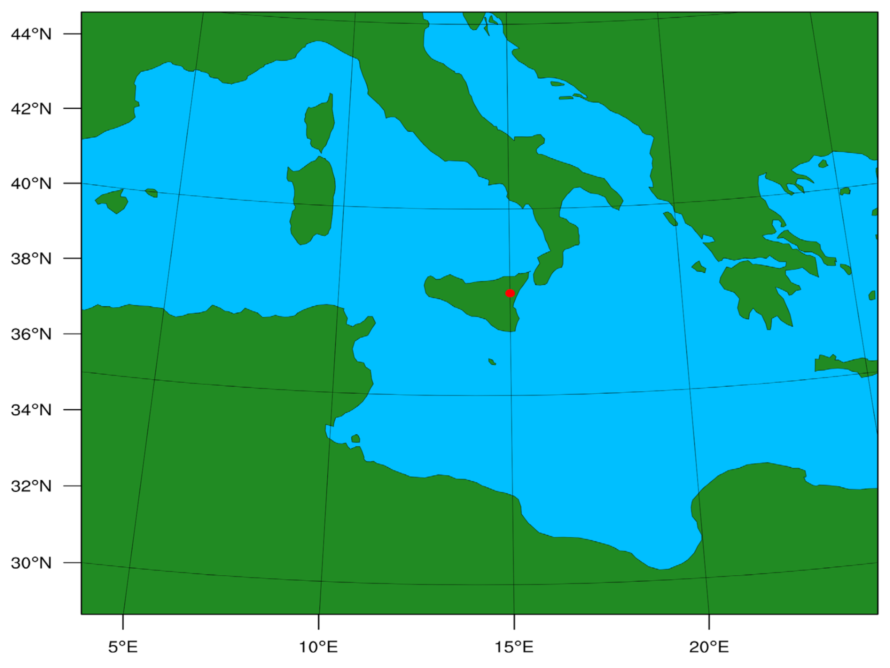
2.1. The 23 November 2013 Etna Paroxysm: Eruption Timeline and Synoptic Conditions

On the morning of 23 November 2013, Etna’s New SE Crater produced the 42nd paroxysmal episode since January 2011. The ash plume top reached up to 12.6 km a.s.l. [35]. The strong wind spread the tephra plume toward NE, generating abundant fallout of bombs up to several kilometers and dispersing fine lapilli all along the Ionian coast of Sicily. Thick fallout caused serious trouble to infrastructures including the highway about 10 km east. Ash fallout was reported in southern Calabria and Puglia regions in southern Italy, and as far as 400 km from the volcano. From thermal images analysis, Bonaccorso et al. [36] inferred a time-averaged-discharge-rate of ~360 m³ s⁻¹, i.e., ~1.6 × 10⁶ m³ of dense-rock equivalent magma volume erupted in just 45 min.

The maps of the geopotential height (NOAA-Global Forecast System: https://www.ncei.noaa.gov/products/weather-climate-models/global-forecast (accessed on 18 February 2021) relating to the isobaric surface at 500 hPa of the day of 23 November 2013 show a large depression circulation that affects much of the central-western Mediterranean (not shown). The pressure minimum off-shore southern France tends to isolate itself in the middle Tyrrhenian Sea. This synoptic framework, in addition to bringing extensive conditions of atmospheric instability over much of Italy, with precipitation also of a stormy nature especially in the Tyrrhenian areas, favored the genesis of intense winds at high altitude. In particular, as shown by the wind speed maps at 300 hPa at the main synoptic hours (Figure 1a at 00:00 UTC, Figure 1b at 06:00 UTC, Figure 1c at 12:00 UTC, and Figure 1d at 18:00 UTC), thanks to the transit of a secondary branch of the Jet Current, Sicily was affected by winds at high altitude, locally even higher than 50 m s⁻¹ (180 km h⁻¹), coming mainly from the south-western quadrants.

The presence of a low-pressure system in the middle of Tyrrhenian Sea, favored a flux of cold air at high altitude over the Mediterranean basin from the Scandinavian Peninsula (not shown in Figure 1). In particular, masses of cold air at the isobaric surface of 850 hPa (about 1500 m above sea level) mostly affected the western sector of Italy at 00:00 UTC. In the following hours of 23 November, the colder air masses affected the entire national territory, extending to a large part of the Adriatic Sea.

2.2. Remote-Sensing Data

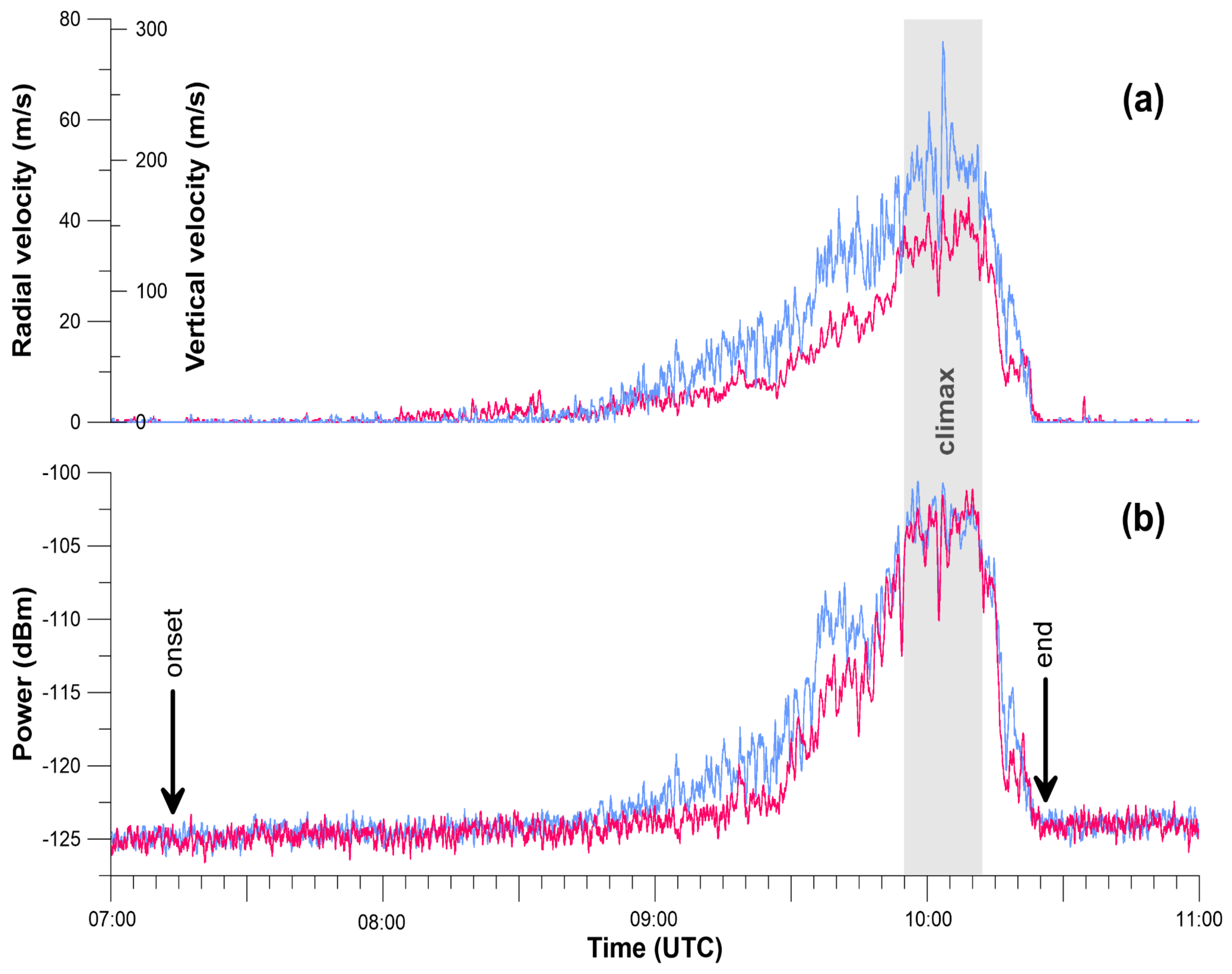
2.2.1. VOLDORAD-2B Doppler Radar System

Etna tephra emissions have been monitored since 2009 using a unique volcano Doppler radar, VOLDORAD-2B, operated jointly by OPGC and INGV-OE from the Montagnola station, 3 km south of the New SE Crater. During the 2011–2015 period, the radar has successfully recorded data from about 50 paroxysms of tephra plumes fed by lava fountains, available from an open-access database of the Observatoire de Physique du Globe de Clermont-Ferrand (http://voldorad.opgc.fr/bddtr.php (accessed on 17 May 2021); [37]). Using a fixed-pointing antenna beam, this 23.5 cm-wavelength pulsed radar sounds 13 atmospheric volumes, 120 m-deep, right above the summit craters. The echo power and radial velocities (level 1 data) are computed from the raw Doppler spectra recorded at intervals of 0.22 s. These unique near-source measurements of the emitted tephra allow maximum ejection velocities at the base of the eruptive column and mass eruption rates (level 2 data) to be determined in real-time [14,15,16,38]. Owing to its capacity for implementation in real-time, we used the methodology of Freret-Lorgeril et al. [15] to compute MER from the product between the echo power and radial velocities measured in the two beam volumes above the New SE Crater, from which the 23 November 2013 paroxysm originated. This product has been shown to be proportional to the MER of tephra passing through the probed volume (MER proxy) and correlates to the observed plume heights for many paroxysms at Etna. Therefore, the VOLDORAD-2B MER proxies could be calibrated with MER derived from the plume model of Degruyter and Bonadonna [39], matching the same plume heights and including wind vertical profiles measured during eruptions.

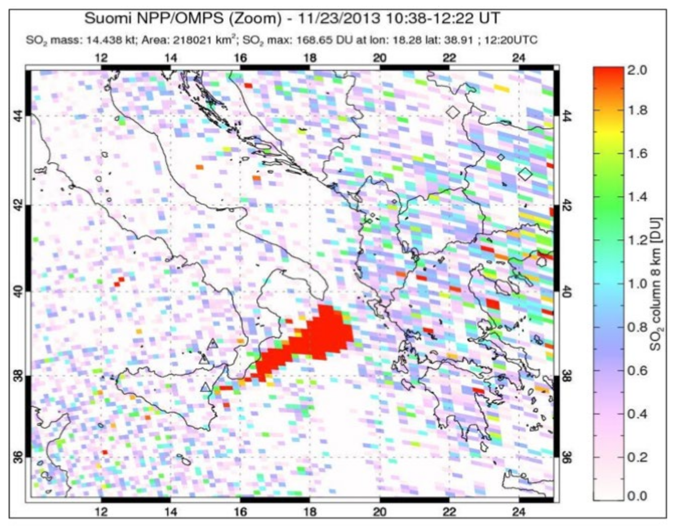
2.2.2. Suomi NPP (OMPS/VIIRS) Data

The Ozone Mapping and Profiler Suite (OMPS) is onboard the joint National Aeronautics and Space Administration/National Oceanic and Atmospheric Administration (NASA/NOAA) Suomi National Polar-orbiting Partnership (Suomi NPP) satellite, launched in October 2011. In particular, the OMPS-NPP L2 NM Aerosol Index swath orbital product provides aerosol index values from the OMPS Nadir-Mapper (NM) instrument. This is actually the official NASA aerosol index product, which replaces the aerosol index found in the OMPS-NPP L2 NM Total Ozone product. The aerosol index is derived from normalized radiances using two wavelength pairs at 340 and 378.5 nm in the ultra-violet spectrum. The dataset is accessible through the NASA Earthdata Search web portal (https://search.earthdata.nasa.gov/search (accessed on 5 May 2021).

The Visible Infrared Imaging Radiometer Suite (VIIRS) is onboard the Suomi NPP and the Joint Polar Satellite System (JPSS) spacecrafts. The VIIRS instrument has 22-spectral bands, covering the spectrum between 0.412 and 12.01 μm, including 16 moderate resolution bands (M-bands) with a spatial resolution of 750 m at nadir, and 5 imaging resolution bands (I-bands) with a 375 m resolution at nadir. The brightness temperature was downloaded from the NOAA-CLASS web portal at https://www.avl.class.noaa.gov/saa/products/welcome (accessed on 6 July 2021) by selecting the VIIRS data records from the Suomi NPP products. The brightness temperature of the thermal infrared channels has been widely used in dust storm monitoring [40] but also to detect volcanic plumes [41].

2.2.3. MSG SEVIRI Images Data

The Spinning Enhanced Visible and InfraRed Imager (SEVIRI: https://www.eumetsat.int/seviri (accessed on 17 May 2021)) is a 12-channel sensor onboard Meteosat Second Generation (MSG) spacecraft. It is a geostationary, meteorological satellite developed by the European Space Agency in close co-operation with the European Organisation for the Exploitation of Meteorological Satellites. Product images are available at a frequency of 1 image/15 min with a pixel resolution of 3 × 3 km at nadir. The HOTVOLC observing system ([42]; https://hotvolc.opgc.fr (accessed on 17 May 2021) is a web-based satellite-data-driven reporting system dedicated to the observation of volcanic products including in real-time. HOTVOLC is a Web-GIS (Geographic Information System) volcano monitoring system developed at the Observatoire de Physique du Globe de Clermont-Ferrand (France). It uses on-site automated ingestion of MSG-SEVIRI geostationary data for direct dissemination on a full web–GIS interface of ready-to-use products characterizing volcanic ash, sulphur dioxide, and lava flow emissions from spectral band combinations. Satellite products are delivered in the form of geo-referenced images (geotiff) tiled on a background map and time series (csv) through an open-access database. Although several elaborated ash products (ash plume altitude, mass, contour) have been made available recently from combinations of thermal infrared channel radiance data, for the 23 November 2013 ash and SO₂ plume, we were able to use only ash RGB composite images from the HOTVOLC archive data combining IR8.7, IR10.8, and IR12.0 channels.

2.2.4. Multi-Satellite Volcanic Sulfur Dioxide Long-Term Global Database

The input parameters for SO₂ were obtained from the Multi-Satellite Volcanic Sulfur Dioxide L4 Long-Term Global Database in its Version 4 (MSVOLSO2L4), which is provided as an ASCII file and available for download at NASA Goddard Earth Sciences Data and Information Services Center (GES DISC) (10.5067/MEASURES/SO2/DATA405). Version 4 [10] is the current version of the dataset and older versions are no longer available. The data represent the best estimates of the volcanic and anthropogenic contribution to global atmospheric SO₂ concentrations. It consists of a long-term database of volcanic SO₂ emission derived from ultraviolet satellite measurements from 31 October 1978 to present, including data from Total Ozone Mapping Spectrometer (TOMS), Ozone Monitoring Instrument (OMI), Ozone Mapping and Profiler Suite (OMPS), and TROPOspheric Monitoring Instrument (TROPOMI) sensors (https://disc.gsfc.nasa.gov/datasets/MSVOLSO2L4_4/summary (accessed on 17 May 2021).

2.3. Model Setup

2.3.1. Numerical Setup

A new specialized module has been implemented inside the Weather Research and Forecasting (WRF) with Chemistry model (WRF-Chem, [31]) that allows simulation of the emission, transport, and settling of aerosols and gases released during volcanic eruptions [8]. Among the WRF-Chem specialized options that are available for the description of the transport of volcanic ash and gas (SO₂), we used the inert tracer options that utilize 10 ash variables and SO₂.

The numerical grid, depicted in Figure 2, has (250, 220) grid points with (dx, dy) = (8, 8) km and dt = 40 secs, upon a Lambert Conformal projection. Simulation started at 00:00 UTC 22 November 2013 and stopped at 00:00 UTC 26 November 2013. Initial and boundary conditions of meteorological variables were obtained from NCAR/NCEP Final Analysis from Global Forecast System (FNL from GFS-ds083.2), which are available every 6 h at a 1° resolution (http://www2.mmm.ucar.edu/wrf/users/download/free_data.html (accessed on 17 February 2021).

About the setting of the WRF physical parameters, the surface layer module corresponds to the Mellor-Yamada-Nakanishi and Niino (MYNN, [43]) scheme (sf_sfclay_physics = 5), the Rapid Update Cycle Land Surface Model [44] was used to represent the land surface interactions (sf_surface_physics = 3) and the MYNN 2.5 level turbulent kinetic energy parameterization was used to describe the planetary boundary layer parameterization (bl_pbl_physics = 5). Short- and long-wave radiation effects were modeled using the Rapid Radiative Transfer Model (RRTMG, [45]) for both short- and long-wave (ra_sw_physics = ra_lw_physics = 4); the two-moment cloud model microphysics scheme of Morrison et al. [46] was used for the treatment of the microphysical processes (mp_physics = 10).

This configuration has been already successfully tested by Rizza et al. [47] and well suited for the study of transport of natural aerosols in the Mediterranean basin.

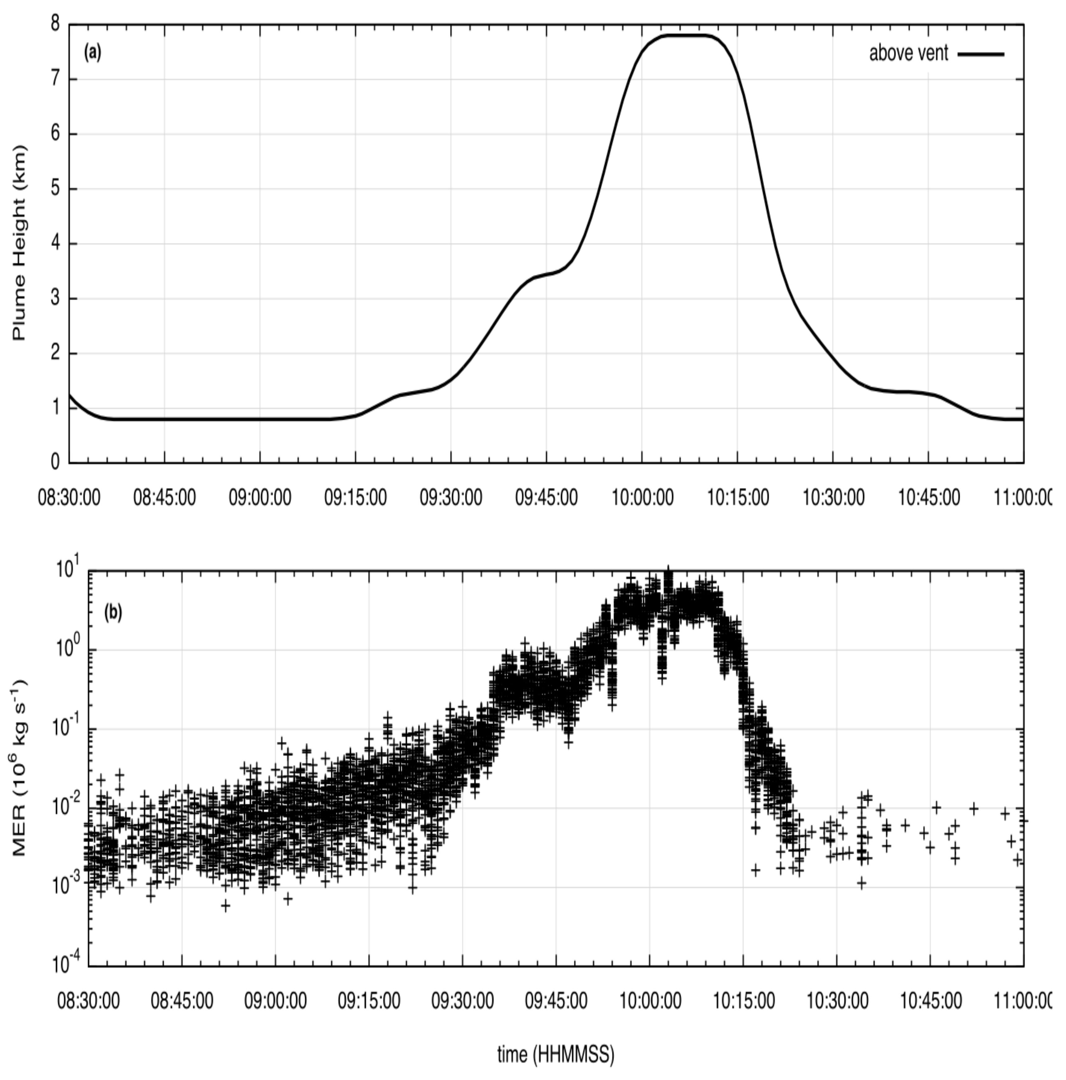
2.3.2. Eruption Source Parameters

The definition of ESP together with the other specific volcanic parameters, namely the volcano location in the grid domain, start and end of each single paroxysm (UTC time), and TGSD, was calculated at the pre-processing level utilizing an NCAR Command Language script. The resulting ASCII file contained all the volcanic information needed at runtime by WRF-Chem. Future releases will consider a unique pre-processing environment also including the elaboration of the raw V2B radar data.

Figure 3 displays the V2B radar echo power and maximum radial velocity records in the two bins above New SE Crater (3 and 4, i.e., at 3135 and 3285 m) on 23 November, integrated over 1.1 s. The onset of continuous tephra emission is detected by the radar with emergent signals at 07:13 UTC, although both echoes and velocities increase strongly after 08:30. They peak and stabilize between 09:55 and 10:14, indicating a climax phase of sustained steady emission lasting 20 min characterized by average vertical velocities of 194 m s⁻¹ (peaks up to 341 m s⁻¹) and about −103 dBm average peak power. Then, the radar signals drop abruptly until the paroxysm ends at 10:26 UTC.

The value of MER [kg s⁻¹] was computed from the level 1 data using the calibration method of Freret-Lorgeril et al. [15]. A total erupted mass (TEM) of 4.7 10⁹ kg was computed from the integration of MER over the duration of the tephra emission totaling 193 min. The climax was found to release 83% of the TEM and to have an MER 8.5 times higher (3.4 × 10⁶ kg s⁻¹) than that of the whole paroxysm (4.0 × 10⁵ kg s⁻¹). It may be notified that the average peak values of the exit velocity (approximately 150 m s⁻¹) and MER (approximately 10⁷) in the climax agree well with an independent analysis performed by Montopoli [48] on the same case study.

The plume height data were measured from the ECV visible camera of Istituto Nazionale di Geofisica e Vulcanologia, Osservatorio Etneo [49] above the vent, so that plume altitude a.s.l. can be obtained by adding about 3.1 km [50].

The V2B raw data were pre-elaborated to be compatible with the WRF-Chem system in particular, they were averaged on a 40 s interval to be incorporated by the numerical model at each time step. The corresponding time series of the plume height (Figure 4a) and MER (Figure 4b) are depicted in Figure 4.

To establish the initial vertical distribution of the erupted mass, it was assumed that the volcanic plume is described by an idealized umbrella shape [51]. In this context, the erupted mass is distributed in the vertical according to the so-called umbrella cloud model. According to the default WRF-Chem configuration [8], it was assumed that 75% of the erupted mass is constrained in the umbrella cloud and 25% below, with a linear distribution from the umbrella base to the vent (Figure 1 of Stuefer et al. [8]).

The elaboration of plume height and V2B data reported in Figure 4a,b suggests that in the paroxysmal phase (09:55–10:14 UTC), the eruption reached an altitude of 11 km (a.s.l.) and then rapidly decreased to around 5 km (a.s.l.) after 10:30 UTC, causing different cloud layers being transported at different altitudes. These results are in agreement (within 1 km) with the analysis of Corradini et al. [35] on the same Etna eruption.

The input parameters for SO₂ were obtained from the MSVOLSO2L4 database (https://disc.gsfc.nasa.gov/datasets/MSVOLSO2L4_4/summary (accessed on 13 May 2021)). The 23 November 2013 eruption that is considered in the present study is catalogued as follows [10]: (i) eruption style = explosive, (ii) eruption volcanic explosivity (VEI) = 2, (iii) observed max plume altitude (a.s.l.) = 11 km, (iv) measured SO₂ mass in kilotons (=1000 metric tons) = 5. Time-varying SO₂ data were elaborated assuming that the SO₂ flux is proportional to the V2B ash MER time series.

In WRF-Chem, as described by Stuefer et al. [8], the TGSD is distributed between 10 bins of aerosol particles with a diameter size range starting from 2 mm down to less than 3.9 μm.

Table 1. Ash particle bin size diameter with corresponding WRF-Chem variable name, modes ($\varphi$), and the mass fractions in percent of total mass recalculated from Poret et al. [4].

Var	Diameter [m]	$\mathit{\varphi }$	E1 [%]
vash_1	(1–2) 10−3	−1:0	16.7
vash_2	(0.5–1) 10−3	0:1	8.35
vash_3	(0.25–0.5) 10−3	1:2	10.4
vash_4	(125–250) 10−6	2:3	12.5
vash_5	(62.5–125) 10−6	3:4	6.25
vash_6	(31.25–62.5$)$ 10−6	4:5	12.5
vash_7	(15.625–31.25) 10−6	5:6	14.6
vash_8	(7.8125–15.625) 10−6	6:7	8.3
vash_9	(3.9065–7.8125) 10−6	7:8	6.2
vash_10	<3.9065 10−6	>8	4.2

gives the selected particle size bins, which were associated with the WRF-Chem variables named vash_1 to vash_10, and the corresponding mass fraction percentage. The particle size diameter (mm) was computed according to the $d=2^{-\varphi }$ function and the corresponding E1 distribution among the 10 bins was recalculated elaborating the eruptive data obtained by Poret et al. [4] for the 23 November 2013 Etna eruption.

Table 2. Eruption source parameters and WRF-Chem chemistry option. ECV and V2B indicate time-varying MER retrieved from the VOLDORAD-2B radar (Figure 3) and plume heights retrieved from a video camera (Figure 4), respectively.

Case	Paroxysm Duration HHMM	wt% Distribution Ash	Column Height a.s.l. [km]	MER Ash [kg s−1]	MER SO2 [g h−1]
run1	0700–1030	E1	11	2.77 × 105	1.67 × 109
run2	0700–1030	E1	ECV	V2B	V2B
run3	0700–1030	E1	4-7-11-7	2.77 × 105	V2B
run4	0955–1015	E1	11	0.65 × 107	V2B
run5	0700–1030	E1	7	4.0 × 105	V2B

shows the ESP and chemistry setup for the two configurations, namely run1 in which ESP are kept constant for the whole paroxysm event (07:13–10:30 UTC) and the run2 configuration that uses time-varying average ESP according to the elaboration of the V2B Doppler radar data reported in Figure 3. The setting chem_opt = 402 corresponds to the inert tracer options that utilizes 10 ash variables (cf. Table 1) and SO₂. In this context, the model sensitivity to the use of transient vs. constant ESP may be evaluated.

3. Results and Discussion

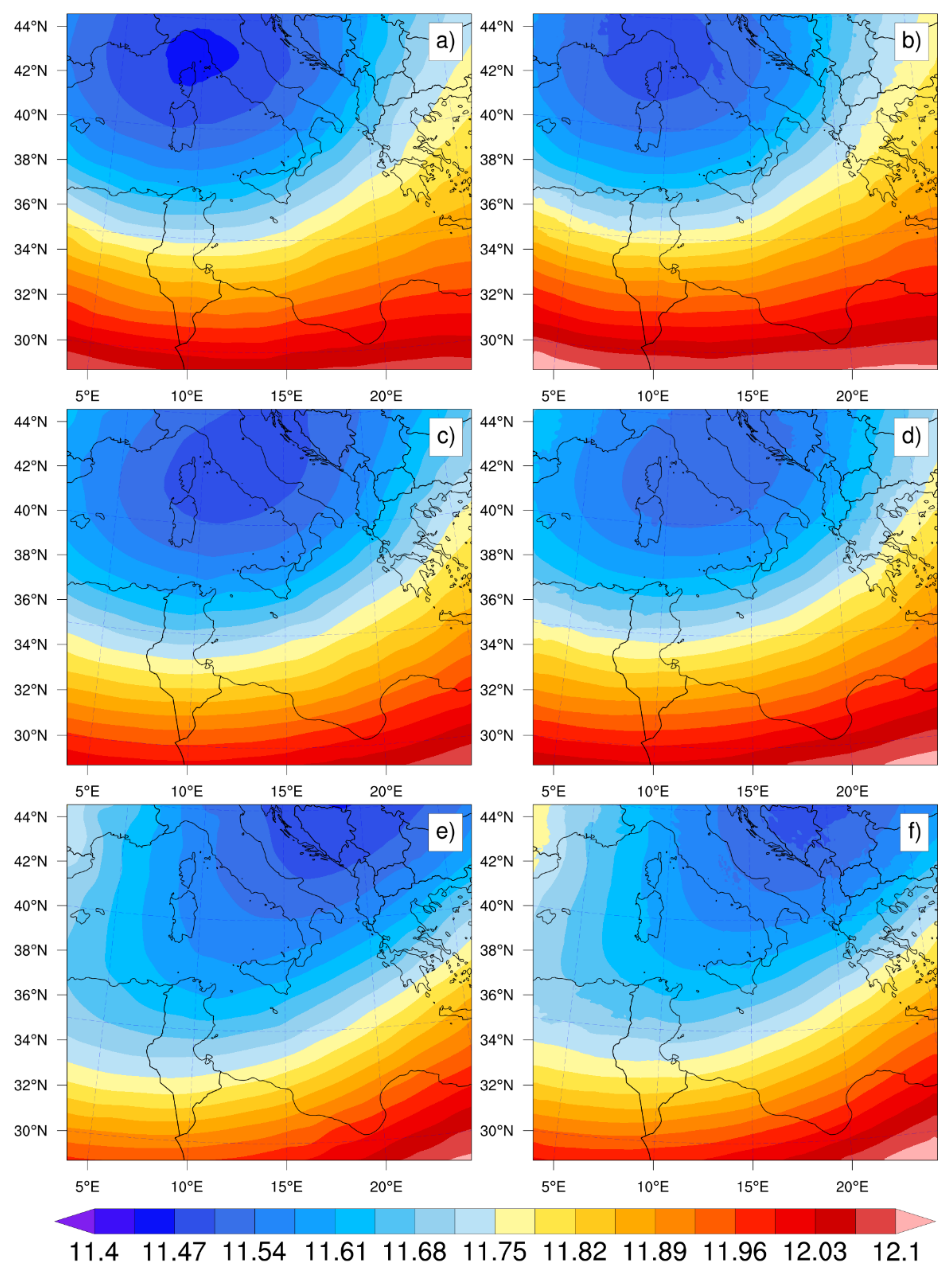
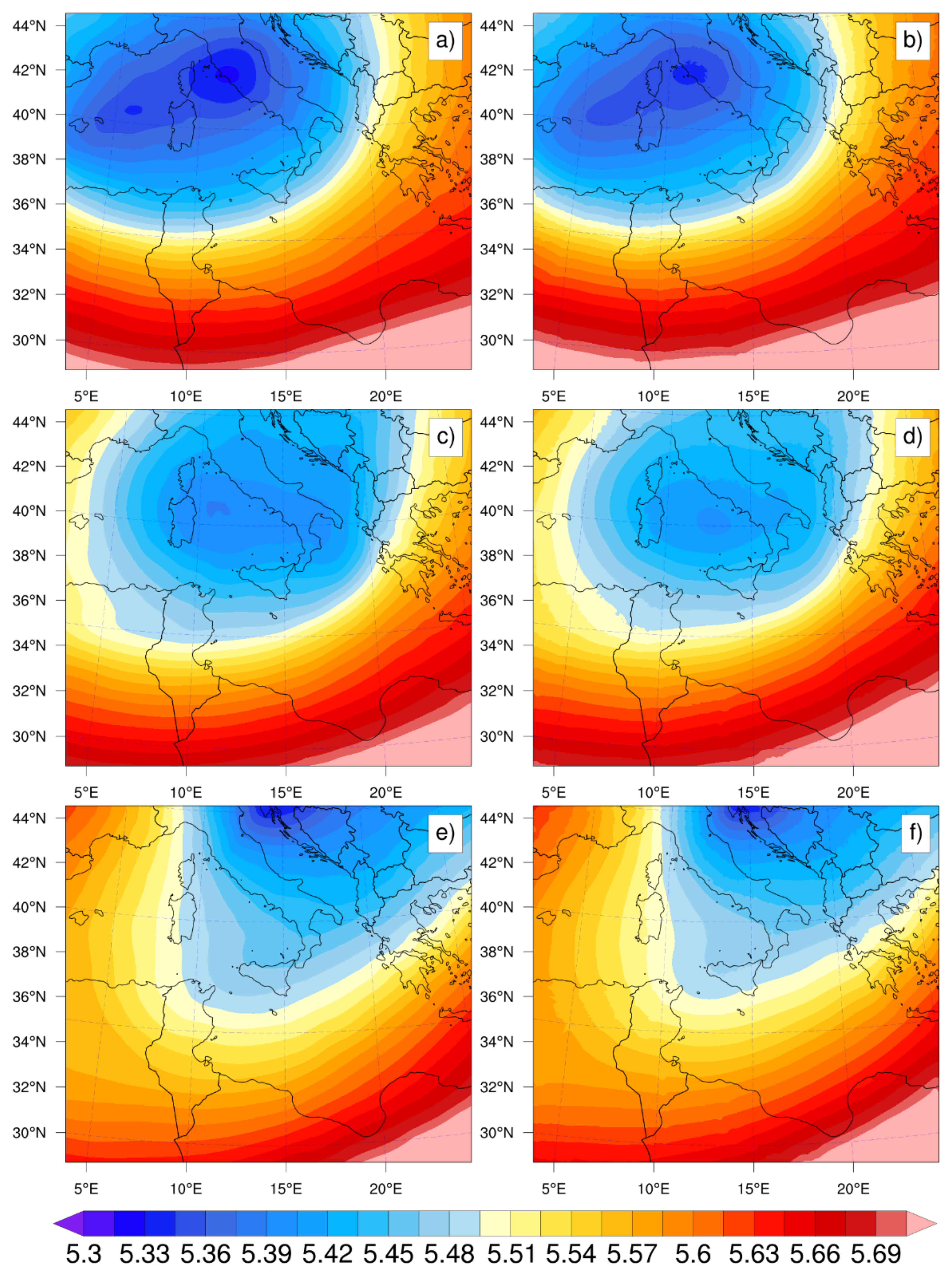
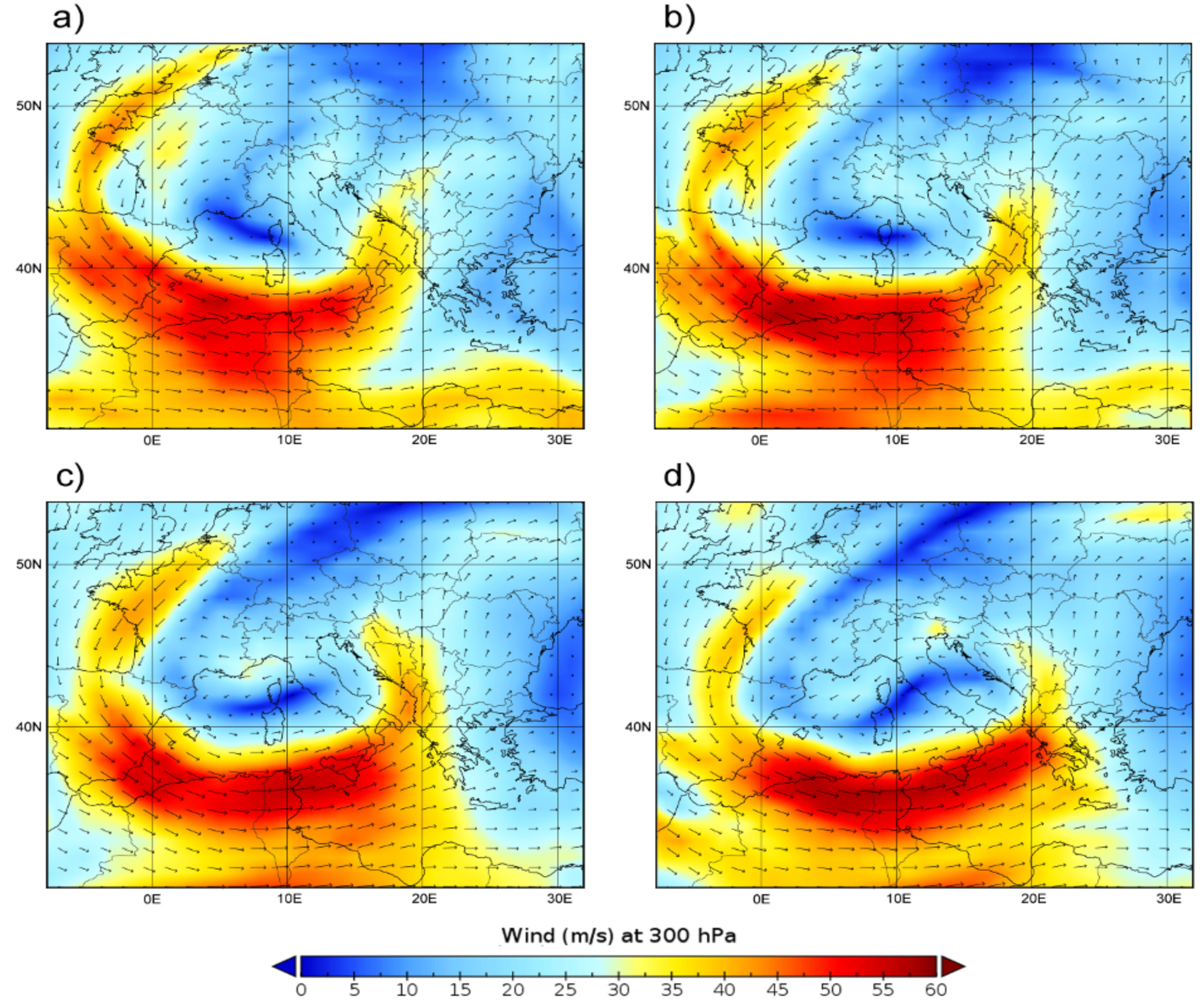
3.1. Geopotential ERA5 vs. WRF

In order to analyze the synoptic conditions in the days following the eruption of Etna, we considered the ERA5 reanalysis [52], which have 137 vertical levels and about 30 km of horizontal resolution. Geopotential fields were obtained by downloading ERA5 hourly data on pressure levels (available from 1979 to present) in netCDF format (https://www.unidata.ucar.edu/software/netcdf/) from the Copernicus Climate datastore (https://cds.climate.copernicus.eu/#!/home (accessed on 13 February 2021).

To compare ERA5 with the WRF-Chem model output fields, we focused on the geopotential height at 500 and 200 hPa. These levels were chosen since they are representative of the upper tropospheric conditions, which determine the long-range transport of the volcanic plumes.

Panels (a, c, e) of Figure 5 and Figure 6 represent ERA5 reanalysis of the geopotential at 200 and 500 hPa (in km), respectively, while panels (b, d, f) represent the WRF-Chem output of the same variable. In each figure, the top, middle, and bottom rows represent snapshots at 12:00 UTC on November 23, 24, and 25, respectively.

At 200 hPa, 23–24 November were both characterized by a pressure minimum localized in northern Italy and dislocating eastward on November 25. This configuration favors an intense cyclonic circulation on the central Mediterranean, with prevailing easterly winds on Sicily and the southern Mediterranean.

As depicted by Figure 6a–d the synoptic configuration at 500 hPa is quite similar; however, at these lower levels, the circulation in the region invested by the volcanic plume (36–40° latitude north and 15–22° longitude east) is slightly different and more oriented northward. These synoptic conditions highlight the different directions taken by the volcanic plume at approximately 12 and 5 km altitude (a.s.l.) as it will be depicted in the next paragraphs.

It is quite evident how the model (panels b, d, f) is able to reproduce the geopotential fields very well at both pressure levels, equally in terms of configuration and intensity.

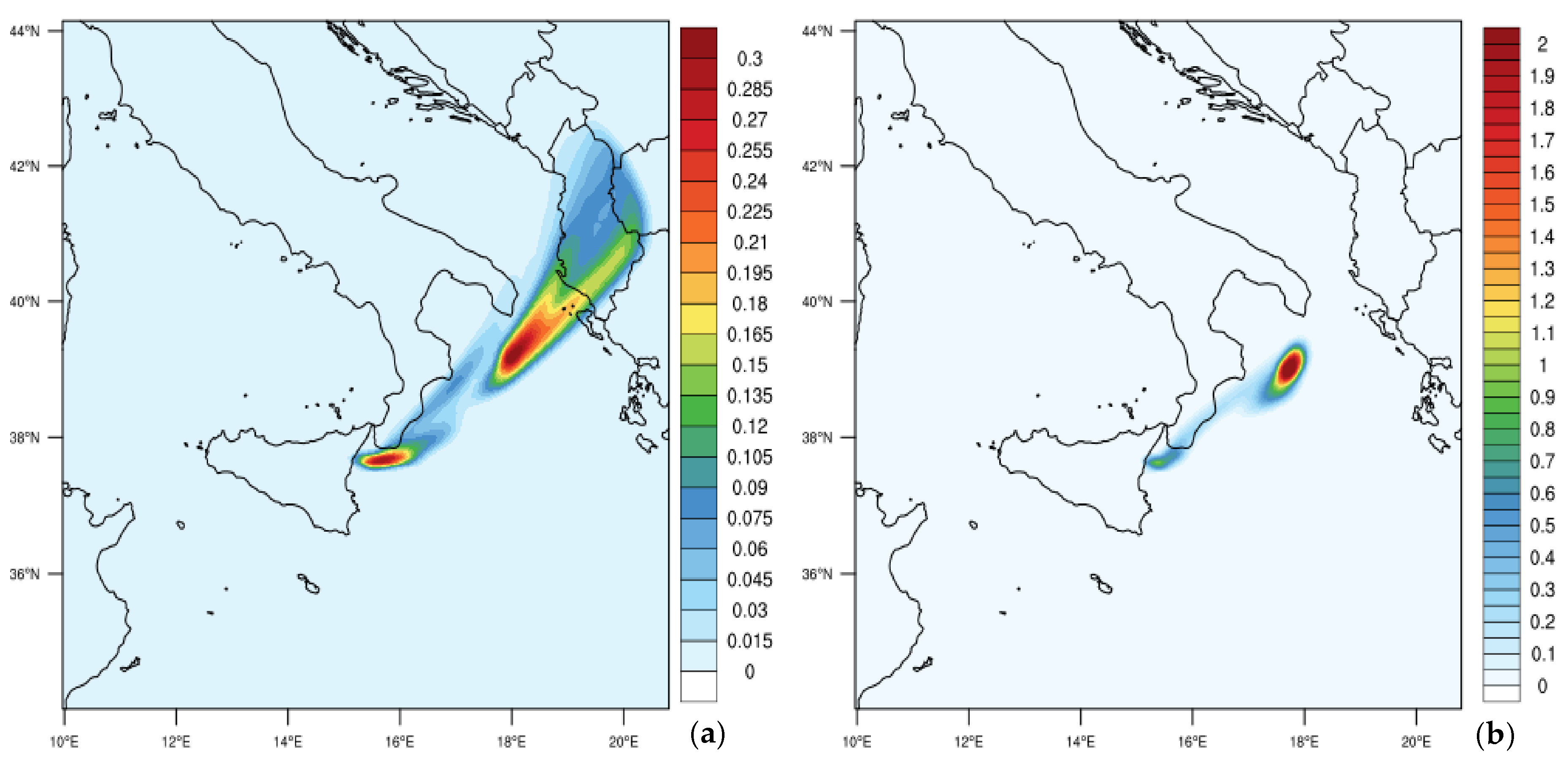
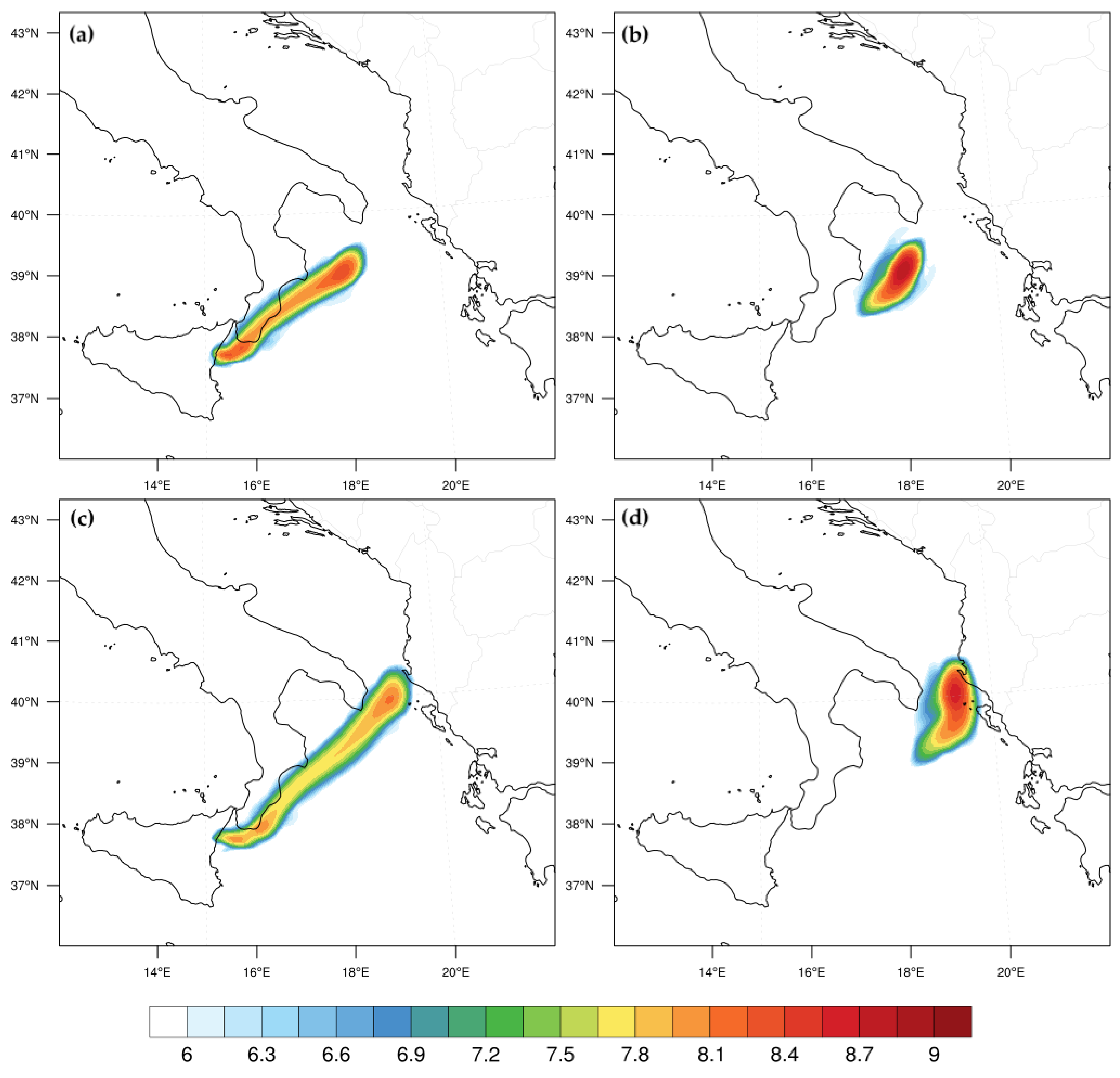
3.2. Comparison for SO₂

The Goddard Space Flight Center (GSFC/NASA), through its Global Sulfur Dioxide Monitoring Home Page (https://so2.gsfc.nasa.gov (accessed on 5 May 2021)), makes data available for downloading, in particular SO₂ eruption alerts, SO₂ near real-time images, and finally archived daily OMI/OMPS/TROPOMI images.

The image reported in Figure 7 is relative to the eruption of 23 November 2013 retrieved from the OMPS sensor onboard the Suomi NPP satellite, which passed in its closest point to Sicily at 12:19 on the same day. This image is relative to the plume distribution about two hours after the eruption climax occurred around 10:00 UTC. As a consequence of the synoptic circulation, described in Section 3.1, the columnar SO₂ distribution after the main eruption is dislocated from Sicily to the Ionian Sea and moving in the north-east direction.

The modeled hourly map at 12:00 UTC (same day) is reported in Figure 8a,b for run1 and run2, respectively. Two important points should be remarked: (i) the volcanic plume at 12:00 UTC for run1 is fragmented into two parts with the farthest portion already passed over the Albanian coast and (ii) the spatial pattern relative to run2 is very similar to OMPS retrievals at the same hour.

This means that according to the run1 configuration, the injection height at 11 km (a.s.l.) for the whole duration of the paroxysm is a wrong assumption that leads to an unrealistic spatial distribution. This is caused by the presence of the ash cloud at the highest tropospheric levels with considerable high wind speed. Contrastingly, the transient ESP under the run2 configuration seems to produce a remarkably closer spatial pattern, both in terms of plume extension and centers of mass.

Moreover, if we consider the columnar density of SO₂, expressed in Dobson Units (DU), according to the simulation outputs, the SO₂ concentration of run2 results in approximately 2.0 DU, which is close the observed value of about 2 DU, while run1 outputs provide a lower value around 0.3 DU. Unfortunately, on the following days (24 and 25 November 2013), there are no satellite retrievals that may be utilized for a further comparison. The closer match of the SO₂ concentration and spatial pattern highlights the need for specifying the appropriate emission height based on time-varying ESP.

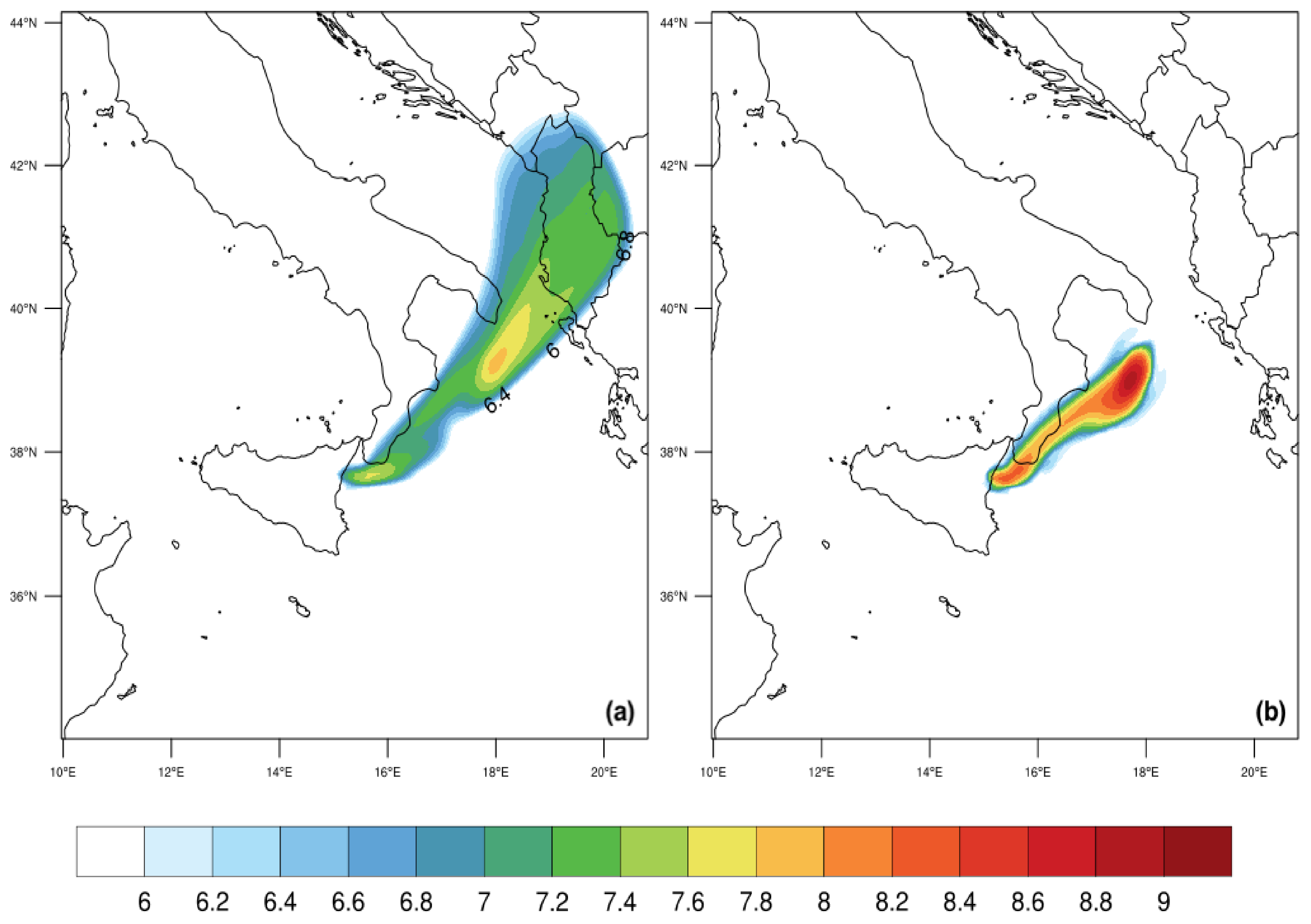
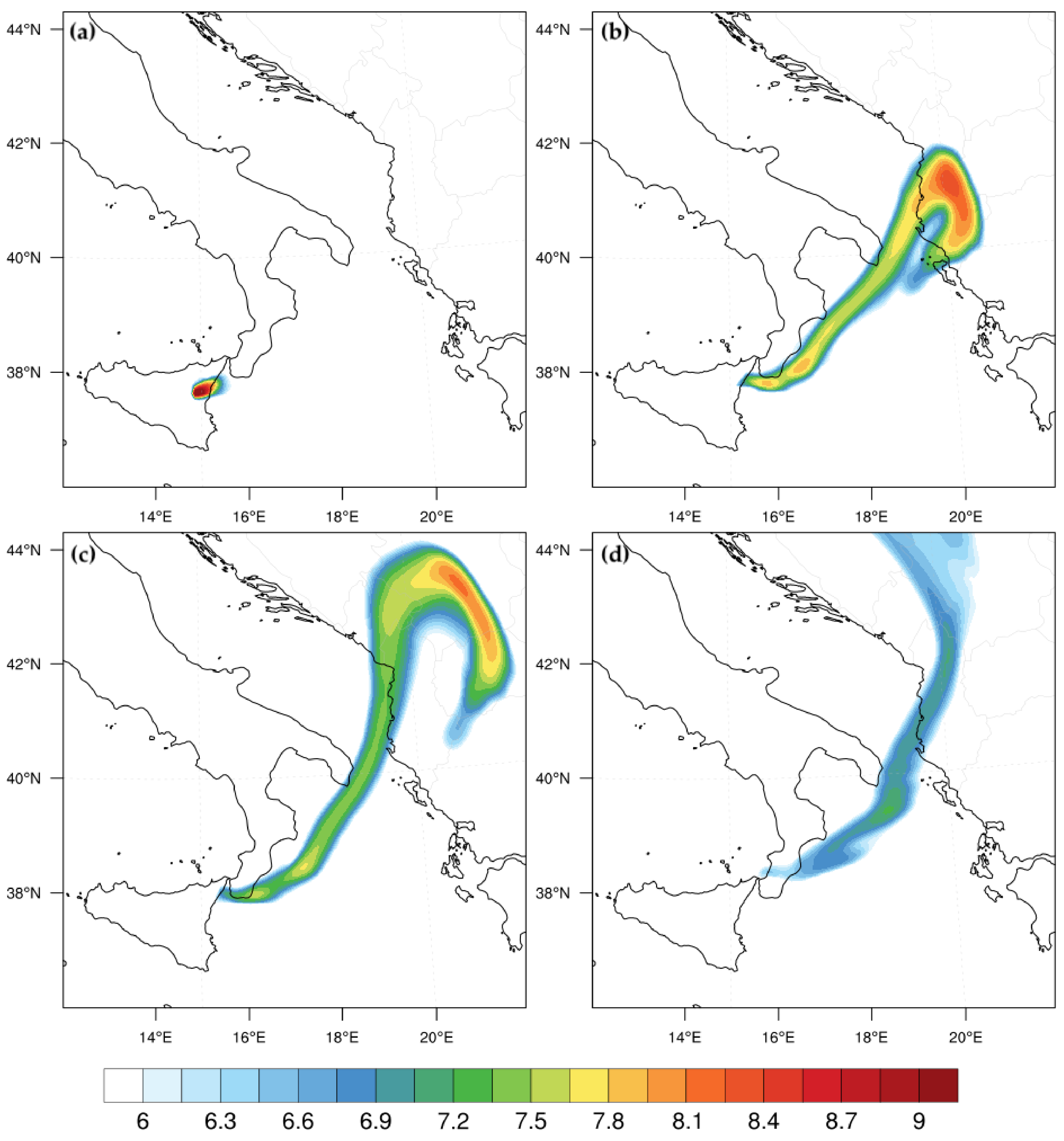
3.3. Comparison for Volcanic Ash

To validate the model predictions with respect to ash, the simulation results were compared with the observed data characterized by the Aerosol Index (AI) that was explicitly developed to detect the presence of aerosols in the air. In particular, the OMPS Aerosol Index layer specifies the presence of ultraviolet (UV)-absorbing particles in the air. In this context, it is useful for identifying and tracking the long-range transport of volcanic ash from volcanic eruptions, but it also may be utilized for other aerosol types, like desert dust, smoke from wildfires, or biomass burning. It is a science parameter of OMPS/National Polar, and derived from normalized radiances using two wavelength pairs at 340 and 378.5 nm. In Figure 9, AI is visualized from Level-2 Swath and 50 × 50 km resolution, over 1 h time coverage around 12:00 UTC on 23 November 2013.

A modeled quantity that could be qualitatively compared with the OMPS/AI is the columnar mass density, which is obtained by considering in each (x, y) grid point the following columnar quantity [53]:

$$Vas{h}_{col}={{\displaystyle \int }}_{zmin}^{zmax}vashT\times {\rho }_{air}dz,$$

(1)

where (zmin = 0 km, zmax = 20 km) are the vertical integration limits, vashT = ${{\displaystyle \sum }}_1^{10}vash\left(i\right)$ represents the sum over all volcanic bins expressed in mixing ratio units (μg kg⁻¹), and ${\rho }_{air}$ is the air density (kg m⁻³). The resulting columnar quantity (Vash_col) is expressed in μg m⁻² and reported in Figure 10a,b in Log₁₀ scale.

Considering that the comparison between Aerosol Index observations (Figure 9) and the modeled columnar mass density (Figure 10) is only qualitative, being performed between two quantities with different units, the very close reproduction of the spatial pattern by the run2 configuration (Figure 10b) at 12:00 UTC on 23 November 2013 is remarkable. In contrast, the extension at the same hour of the modeled plume over Albania and beyond in the run1 simulation (Figure 10a) reveals the unrealistic presence of volcanic ash at a high tropospheric level as far as 20 km beyond the downwind extension limit of the observed aerosols. This means that the use of averaged parameters to describe the eruptive column may lead to very substantial errors in the time and space dispersion of volcanic ash and aerosols. In particular, the optimal comparison of observations and run2 simulation is mainly the result of the appropriate specification of the time-varying MER and transient injection height. It is worth mentioning that the use of the FALL3D model as depicted by Poret et al. [4] on the same paroxysm provided comparable results, as depicted by their Figure 11 (panels a, b).

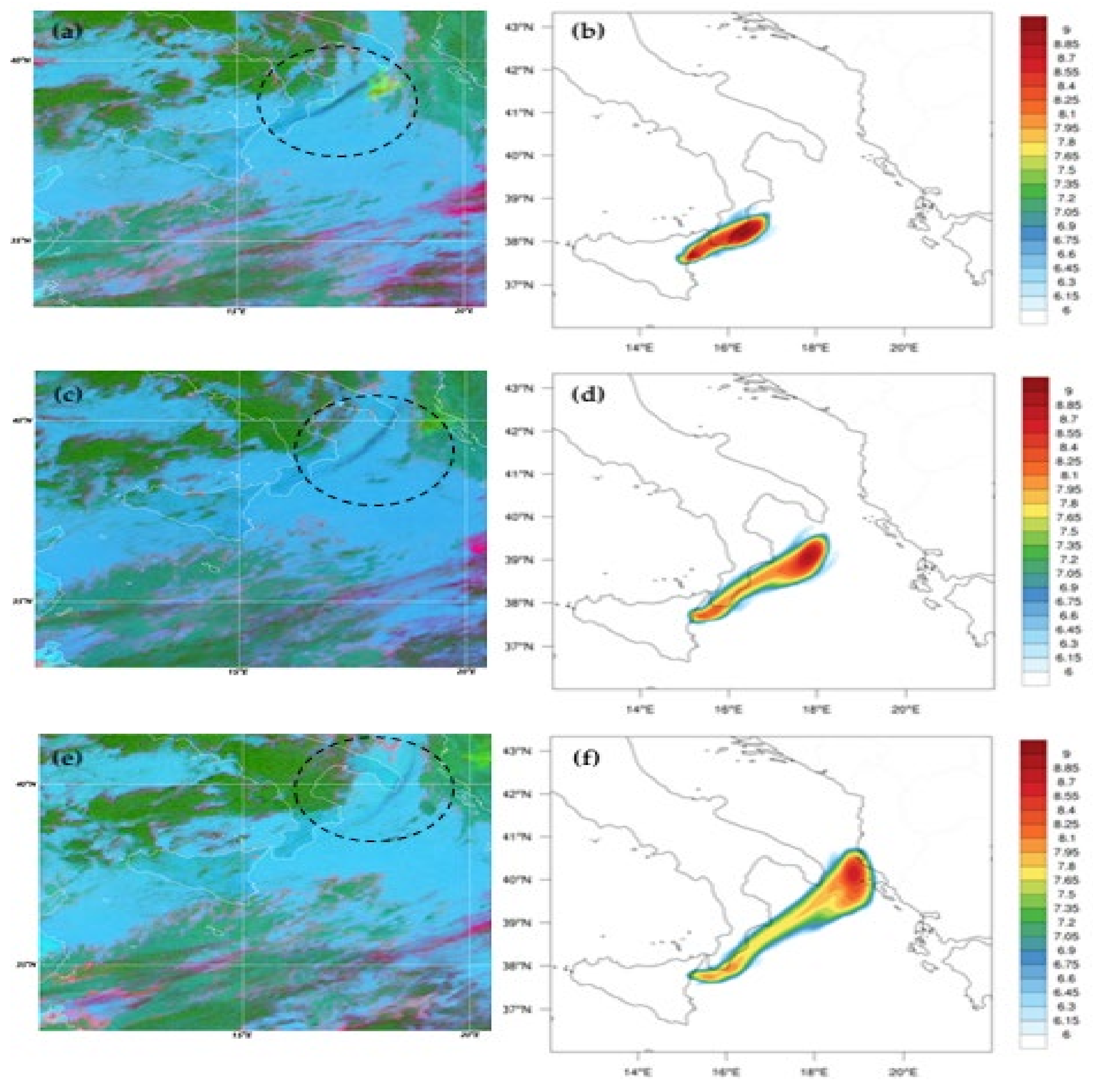
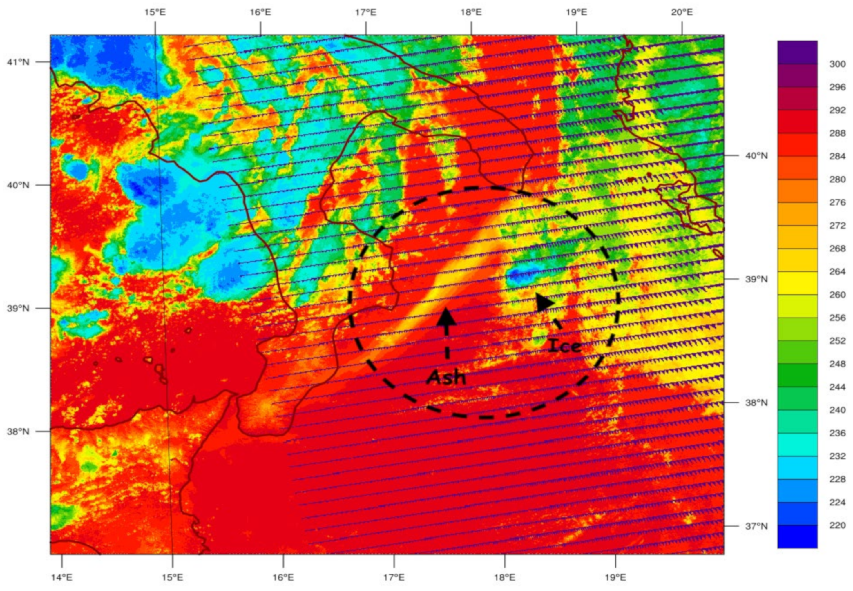
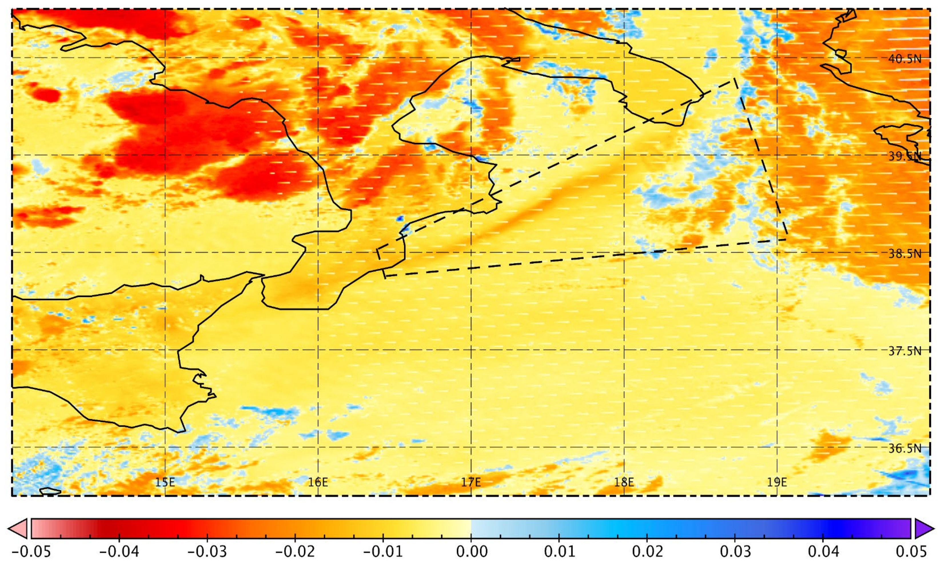
3.4. Comparison with MSG-SEVIRI Data

In this section, we compare the MSG-SEVIRI RGB composite images from HOTVOLC with the outputs of the WRF-Chem model under the run2 configuration. Figure 11 represents the plume snapshots at 11:00 (upper row), 12:00 (central row), and 13:00 UTC (lower row) on 23 November 2013. Panels (a, c, e) denote the RGB satellite images while panels (b, d, f) display the WRF-Chem outputs from the run2 configuration. In panels (a, c, e), the ash aerosols are colored in blue, whereas ice and water hydrometeors are colored in red and light green, respectively. The plume is traveling quite fast, being driven by north-east winds at almost 120 km h⁻¹, reaching Albania at 13:00 UTC.

The RGB images show a narrow volcanic plume denoted by the blue filament inside the black dotted oval that is “headed” by a red/green spot representing the presence of water/ice hydrometeors transported with the plume at 11:00 UTC (Figure 11a). This red/green spot is moving eastward in the following hours at 12:00 and 13:00 UTC (Figure 11c,e) while the rest of the plume, composed by ash aerosols, is moving in the north-east direction.

This probably indicates that a portion of the ash plume, depending on the local relative humidity and temperature, is ice nucleated and transformed into non-precipitating hydrometeors. This requires a microphysical-aerosol coupler [54] to be further investigated. Once more, it is important to remark on the optimal performance of the WRF-Chem model using time-varying ESP in input (run2 configuration), as depicted by panels b, d, and f of Figure 11.

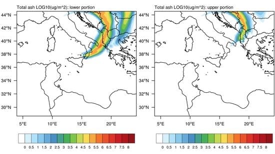
3.5. Ash Transport at Vertical Layers

To analyze the plume transport at different heights, we have split the plume into two parts. In Equation (1), the lower portion is calculated between zmin = 0 km and zmax = 8 km (a.s.l.) and the upper portion between zmin = 8 km (a.s.l.) and zmax = 12 km (a.s.l.). In this discussion, we only consider WRF-Chem outputs under the run2 configuration as it demonstrates superior performances compared with the run1 setup.

The upper panels of Figure 12a,b are the snapshots at 12:00 UTC while the lower panels (c, d) refer to 13:00 UTC of 23 November. Panels (a, c) are the vertical integrals between 0 and 8 km and panels (b, d) between 8 and 12 km (a.s.l.).

In the lower portion Figure 12a,c, we can observe typical thin and narrow volcanic plume stretching very rapidly in the north-east direction and reaching Albania at 13:00 UTC, while the upper plume portion (panels b, d) that contains the largest quantity of the ash load (~10⁸–10⁹ μg m⁻²) is transported in a more easterly direction. This behavior of the volcanic plume is confirmed by Figure A1 (Appendix A) showing the plume splitting around 14:00 UTC (Figure A1b). This is compatible with the geopotentials at 200 and 500 hPa, shown in Section 3.1. In particular, the 200 and 500 hPa geopotentials at 12:00 UTC (Figure 5b and Figure 6b, respectively) show small differences in wind direction at these two pressure heights.

These results are in agreement with the satellite data (MSG-SEVIRI) analysis of Poret et al. [4] highlighting the presence of a north-eastern volcanic ash cloud at about 6 km (a.s.l.) and a volcanic ice cloud at 11 km (a.s.l.).

Finally, Figure 13 reports the brightness temperature from the channel I5 (BTI5) at 11.5 μm of the NPP-VIIRS sensor. It reveals the location of the ash and ice plumes, respectively. The analysis of BTI5 shows that the ash plume was at around 260–270 K at approximately 3 km (a.s.l.), while the ice plume was at $~$220 K at 9 km (a.s.l.). This is confirmed by Figure A2 in Appendix B, obtained by analyzing the brightness temperature difference between the two thermal infrared VIIRS channels B15 and B16 at 11.763 and 12.03 μm, respectively. The dotted region highlights the presence of ash with thermal difference DT < 0 [41] and ice with DT > 0.

These results likely indicate that a portion of the ash plume, depending on the local relative humidity and temperature, can act as ice-nucleating particles [34]. This requires a microphysical-aerosol coupler [54,55] to be further investigated with the WRF-Chem model.

4. Conclusions

In this work, we investigated the effects of variable eruption source parameters on volcanic plume transport of the Mount Etna paroxysm of 23 November 2013. It represents a further application of the WRF-Chem model for Mount Etna following Rizza et al. [32]. Concerning the model setup, the raw data obtained from the V2B Doppler radar system were elaborated at the WRF-Chem pre-processing level. This allowed the inclusion of the transient and fluctuating nature of the volcanic emissions to accurately model atmospheric dispersion of ash/gas, pointing to the exact definition of the most critical parameters, such as paroxysm onset and end, column height, total grain size distribution, and mass eruption rate (MER).

This joint approach between an online coupled chemical transport model (CTM) like WRF-Chem and the data from the V2B Doppler radar system represents an innovative development of current volcanic ash transport and dispersion models as it considers the two-way feedback for all the processes (meteo, chemistry, and physics) at the time step level, in a context of time-varying eruption source parameters (ESPs). The meteorology is part of the system and consequently there is no need to extrapolate/interpolate external fields for both passive and active tracers.

The system was evaluated considering a Mount Etna eruption that has been largely investigated by the scientific community. This paroxysm was characterized by a north-east rapid transport of ash and gas, caused by a low-pressure system in northern Italy.

Two WRF-Chem configurations were evaluated: the first one with the climax values for the ESP, like in Rizza et al. [32], and the second with the time-varying ESP according to the MER time profiles recorded by the V2B radar. It was shown that the second configuration produces a considerably better comparison with satellite retrievals (Ozone Mapping and Profiler Suite, Meteosat Second-Generation Spinning Enhanced Visible and Infrared Imager, and Visible Infrared Imaging Radiometer Suite). To verify the role of the initial column height, three additional runs were performed and discussed in Appendix C. The relative analysis indicated that it is fundamental to describe with “great realism” MER and column height parameters during the climax phase of paroxysm. The “old style” characterization of the ESP based on eruptive average values does not adequately reproduce the transport of ash particles after the eruption. These results suggest the “main avenue” for future development of coupled CTM-radar systems, namely their full integration, at the level of the model time step, to describe all the processes involved with reactive volcanic tracers.

In this work and in the work by Rizza et al. [32], we demonstrated that the model WRF-Chem may be utilized for forecast simulations of meteorology and ash/gas dispersion of Mount Etna emissions. In addition, it may also be particularly useful to better understand its impact on the meteorological phenomena over the whole Mediterranean area.

Specific future upgrade of the WRF-Chem model aiming to further increase the accuracy of the predictions are currently underway, namely (i) a new subroutine to describe the initial column height from V2B-derived MER and 1-D column models, and (ii) a new gravitational settling scheme to consider large ash particles.

The principal suggestion for future research in the area of volcanic ash dispersion is to include a high-resolution imbedded model of volcanic plume. It is likely that the dedicated volcanic plume model will allow explicit simulation of particle coagulation and the transition between the vertical transport mode in the cloud and the predominantly horizontal mode associated with the flow resolved by the WRF-Chem.

All these considerations indicate that simulations would be achievable in near real-time in the future using VOLDORAD-2B monitoring data as input. Concluding this initial setup phase, the new system is scheduled to run in near real-time at the University of Messina (Department of Mathematical and Informatics Sciences) and will be able to provide hazard evaluations to governmental agencies immediately following Mount Etna’s explosive eruptions.

References

1. Robock, A. Volcanic eruptions and climate. Rev. Geophys. 2000, 38, 191–219. [Google Scholar] [CrossRef]
2. Durant, A.J.; Bonadonna, C.; Horwell, C. Atmospheric and Environmental Impacts of Volcanic Particulates. Elements 2010, 6, 235–240. [Google Scholar] [CrossRef]
3. Guffanti, M.; Casadevall, T.; Budding, K. Encounters of Air-Craft with Volcanic Ash Clouds: A Compilation of Known Incidents, 1953–2009, US Geological Survey Data Series 545, 1.0, 1. Available online: http://pubs.usgs.gov/ds/545 (accessed on 23 November 2020).
4. Poret, M.; Corradini, S.; Merucci, L.; Costa, A.; Andronico, D.; Montopoli, M.; Vulpiani, G.; Freret-Lorgeril, V. Reconstructing volcanic plume evolution integrating satellite and ground-based data: Application to the 23 November 2013 Etna eruption. Atmos. Chem. Phys. Discuss. 2018, 18, 4695–4714. [Google Scholar] [CrossRef] [Green Version]
5. Prata, A.T.; Dacre, H.F.; Irvine, E.A.; Mathieu, E.; Shine, K.P.; Clarkson, R.J. Calculating and communicating ensemble-based volcanic ash dosage and concentration risk for aviation. Meteorol. Appl. 2018, 26, 253–266. [Google Scholar] [CrossRef] [Green Version]
6. Folch, A.; Costa, A.; Macedonio, G. FPLUME-1.0: An integral volcanic plume model accounting for ash aggregation. Geosci. Model Dev. 2016, 9, 431–450. [Google Scholar] [CrossRef] [Green Version]
7. Vitturi, M.D.M.; Pardini, F. PLUME-MoM-TSM 1.0.0: A volcanic column and umbrella cloud spreading model. Geosci. Model Dev. 2021, 14, 1345–1377. [Google Scholar] [CrossRef]
8. Stuefer, M.; Freitas, S.R.; Grell, G.; Webley, P.; Peckham, S.; McKeen, S.A.; Egan, S.D. Inclusion of ash and SO2 emissions from volcanic eruptions in WRF-Chem: Development and some applications. Geosci. Model Dev. 2013, 6, 457–468. [Google Scholar] [CrossRef] [Green Version]
9. Muser, L.O.; Hoshyaripour, G.A.; Bruckert, J.; Horváth, A.; Malinina, E.; Wallis, S.; Prata, F.J.; Rozanov, A.; von Savigny, C.; Vogel, H.; et al. Particle aging and aerosol–radiation interaction affect volcanic plume dispersion: Evidence from the Raikoke 2019 eruption. Atmos. Chem. Phys. 2020, 20, 15015–15036. [Google Scholar] [CrossRef]
10. Carn, S. Multi-Satellite Volcanic Sulfur Dioxide L4 Long-Term Global Database V4, Greenbelt, MD, USA, Goddard Earth Science Data and Information Services Center (GES DISC). Available online: https://disc.gsfc.nasa.gov/datasets/MSVOLSO2L4_4/summary (accessed on 20 April 2021).
11. Branca, S.; Del Carlo, P. Types of eruptions of Etna volcano AD 1670–2003: Implications for short-term eruptive behaviour. Bull. Volcanol. 2005, 67, 732–742. [Google Scholar] [CrossRef]
12. Scollo, S.; Coltelli, M.; Bonadonna, C.; Del Carlo, P. Tephra hazard assessment at Mt. Etna (Italy). Nat. Hazards Earth Syst. Sci. 2013, 13, 3221–3233. [Google Scholar] [CrossRef] [Green Version]
13. Andronico, D.; Scollo, S.; Caruso, S.; Cristaldi, A. The 2002–03 Etna explosive activity: Tephra dispersal and features of the deposits. J. Geophys. Res. Space Phys. 2008, 113, B04209. [Google Scholar] [CrossRef] [Green Version]
14. Donnadieu, F.; Freville, P.; Hervier, C.; Coltelli, M.; Scollo, S.; Prestifilippo, M.; Valade, S.; Rivet, S.; Cacault, P. Near-source Doppler radar monitoring of tephra plumes at Etna. J. Volcanol. Geotherm. Res. 2016, 312, 26–39. [Google Scholar] [CrossRef]
15. Freret-Lorgeril, V.; Donnadieu, F.; Scollo, S.; Provost, A.; Fréville, P.; Guéhenneux, Y.; Hervier, C.; Prestifilippo, M.; Coltelli, M. Mass Eruption Rates of Tephra Plumes during the 2011–2015 Lava Fountain Paroxysms at Mt. Etna From Doppler Radar Retrievals. Front. Earth Sci. 2018, 6, 73. [Google Scholar] [CrossRef]
16. Marzano, F.S.; Mereu, L.; Scollo, S.; Donnadieu, F.; Bonadonna, C. Tephra Mass Eruption Rate from X-Band and L-Band Microwave Radars during the 2013 Etna Explosive Lava Fountain. IEEE Trans. Geosci. Remote Sens. 2020, 58, 3314–3327. [Google Scholar] [CrossRef]
17. Peterson, R.A.; Dean, K.G. Forecasting exposure to volcanic ash based on ash dispersion modeling. J. Volcanol. Geotherm. Res. 2008, 170, 230–246. [Google Scholar] [CrossRef]
18. Folch, A.; Costa, A.; Macedonio, G. FALL3D: A computational model for transport and deposition of volcanic ash. Comput. Geosci. 2009, 35, 1334–1342. [Google Scholar] [CrossRef]
19. Skamarock, W.; Klemp, J.; Dudhia, J.; Gill, D.; Barker, D.; Wang, W. A Description of the Advanced Research WRF Version 2; No. NCAR/TN-468+STR; NCAR Scientific Divisions, University Corporation of Atmospheric Research: Boulder, CO, USA, 2005. [CrossRef]
20. Skamarock, W.C.; Klemp, J.B.; Dudhia, J.; Gill, D.O.; Barker, D.M.; Wang, W.; Powers, J.G. A Description of the Advanced Research WRF Version 3; NCAR Scientific Divisions: Boulder, CO, USA, 2008; NCAR Technical note-475 + STR.
21. Collini, E.; Osores, M.S.; Folch, A.; Viramonte, J.G.; Villarosa, G.; Salmuni, G. Volcanic ash forecast during the June 2011 Cordón Caulle eruption. Nat. Hazards 2012, 66, 389–412. [Google Scholar] [CrossRef]
22. Draxler, R.R.; Hess, G.D. An overview of the HYSPLIT_4 modeling system of trajectories, dispersion, and deposition. Aust. Meteor. Mag. 1998, 47, 295–308. [Google Scholar]
23. Jones, A.R.; Thomson, D.J.; Hort, M.; Devenish, B. The U.K. Met Office’s next-generation atmospheric dispersion model, NAME III’. In Air Pollution Modeling and Its Application XVII., Proceedings of the 27 NATO/CCMS International Technical Meeting on Air Pollution Modeling and Its Application, Banff, Canada, 24–29 October 2004; Borrego, C., Norman, A.-L., Eds.; Springer: Boston, MA, USA, 2007; pp. 580–589. [Google Scholar] [CrossRef]
24. Searcy, C.; Dean, K.G.; Stringer, B. PUFF: A volcanic ash tracking and prediction model. J. Volcanol. Geotherm. Res. 1998, 80, 1–16. [Google Scholar] [CrossRef]
25. Plu, M.; Bigeard, G.; Sič, B.; Emili, E.; Bugliaro, L.; El Amraoui, L.; Guth, J.; Josse, B.; Mona, L.; Piontek, D. Modelling the volcanic ash plume from Eyjafjallajökull eruption (May 2010) over Europe: Evaluation of the benefit of source term improvements and of the assimilation of aerosol measurements. Nat. Hazards Earth Syst. Sci. Discuss. 2021. [Google Scholar] [CrossRef]
26. Devenish, B.J.; Francis, P.; Johnson, B.T.; Sparks, R.S.J.; Thomson, D.J. Sensitivity analysis of dispersion modeling of volcanic ash from Eyjafjallajökull in May 2010. J. Geophys. Res. Space Phys. 2012, 117. [Google Scholar] [CrossRef]
27. Webster, H.N.; Thomson, D.J.; Johnson, B.T.; Heard, I.P.C.; Turnbull, K.; Marenco, F.; Kristiansen, N.I.; Dorsey, J.; Minikin, A.; Weinzierl, B.; et al. Operational prediction of ash concentrations in the distal volcanic cloud from the 2010 Eyjafjallajökull eruption. J. Geophys. Res. 2012, 117. [Google Scholar] [CrossRef] [Green Version]
28. Folch, A.; Costa, A.; Basart, S. Validation of the FALL3D ash dispersion model using observations of the 2010 Eyjafjallajökull volcanic ash clouds. Atmos. Environ. 2012, 48, 165–183. [Google Scholar] [CrossRef]
29. Mailler, S.; Menut, L.; Khvorostyanov, D.; Valari, M.; Couvidat, F.; Siour, G.; Turquety, S.; Briant, R.; Tuccella, P.; Bessagnet, B.; et al. CHIMERE-2017: From urban to hemispheric chemistry-transport modeling. Geosci. Model Dev. 2017, 10, 2397–2423. [Google Scholar] [CrossRef] [Green Version]
30. Lachatre, M.; Mailler, S.; Menut, L.; Turquety, S.; Sellitto, P.; Guermazi, H.; Salerno, G.; Caltabiano, T.; Carboni, E. New strategies for vertical transport in chemistry transport models: Application to the case of the Mount Etna eruption on 18 March 2012 with CHIMERE v2017r4. Geosci. Model Dev. 2020, 13, 5707–5723. [Google Scholar] [CrossRef]
31. Grell, G.A.; Peckham, S.E.; Schmitz, R.; McKeen, S.A.; Frost, G.; Skamarock, W.C.; Eder, B. Fully coupled “online” chemistry within the WRF model. Atmos. Environ. 2005, 39, 6957–6975. [Google Scholar] [CrossRef]
32. Rizza, U.; Brega, E.; Caccamo, M.; Castorina, G.; Morichetti, M.; Munaò, G.; Passerini, G.; Magazù, S. Analysis of the ETNA 2015 Eruption Using WRF–Chem Model and Satellite Observations. Atmosphere 2020, 11, 1168. [Google Scholar] [CrossRef]
33. Egan, S.D.; Stuefer, M.; Webley, P.W.; Lopez, T.; Cahill, C.F.; Hirtl, M. Modeling volcanic ash aggregation processes and related impacts on the April–May 2010 eruptions of Eyjafjallajökull volcano with WRF-Chem. Nat. Hazards Earth Syst. Sci. 2020, 20, 2721–2737. [Google Scholar] [CrossRef]
34. Maters, E.C.; Dingwell, D.B.; Cimarelli, C.; Müller, D.; Whale, T.F.; Murray, B.J. The importance of crystalline phases in ice nucleation by volcanic ash. Atmos. Chem. Phys. Discuss. 2019, 19, 5451–5465. [Google Scholar] [CrossRef] [Green Version]
35. Corradini, S.; Montopoli, M.; Guerrieri, L.; Ricci, M.; Scollo, S.; Merucci, L.; Marzano, F.S.; Pugnaghi, S.; Prestifilippo, M.; Ventress, L.J.; et al. A Multi-Sensor Approach for Volcanic Ash Cloud Retrieval and Eruption Characterization: The 23 November 2013 Etna Lava Fountain. Remote Sens. 2016, 8, 58. [Google Scholar] [CrossRef] [Green Version]
36. Bonaccorso, A.; Calvari, S.; Linde, A.; Sacks, S. Eruptive processes leading to the most explosive lava fountain at Etna volcano: The 23 November 2013 episode. Geophys. Res. Lett. 2014, 41, 4912–4919. [Google Scholar] [CrossRef]
37. Donnadieu, F.; Freville, P.; Rivet, S.; Hervier, C.; Cacault, P. The Volcano Doppler Radar Data Base of Etna (VOLDORAD-2B); Université Clermont Auvergne CNRS: Clermont-Ferrand, France, 2015. [Google Scholar] [CrossRef]
38. Freret-Lorgeril, V.; Bonadonna, C.; Corradini, S.; Donnadieu, F.; Guerrieri, L.; Lacanna, G.; Marzano, F.; Mereu, L.; Merucci, L.; Ripepe, M.; et al. Examples of Multi-Sensor Determination of Eruptive Source Parameters of Explosive Events at Mount Etna. Remote Sens. 2021, 13, 2097. [Google Scholar] [CrossRef]
39. Degruyter, W.; Bonadonna, C. Improving on mass flow rate estimates of volcanic eruptions. Geophys. Res. Lett. 2012, 39. [Google Scholar] [CrossRef] [Green Version]
40. Chen, B.; Zhang, P.; Zhang, B.; Jia, R.; Zhang, Z.; Wang, T.; Zhou, T. An overview of passive and active dust detection methods using satellite measurements. J. Meteorol. Res. 2014, 28, 1029–1040. [Google Scholar] [CrossRef]
41. Prata, A.J. Infrared radiative transfer calculations for volcanic ash clouds. Geophys. Res. Lett. 1989, 16, 1293–1296. [Google Scholar] [CrossRef]
42. Gouhier, M.; Guéhenneux, Y.; Labazuy, P.; Cacault, P.; Decriem, J.; Rivet, S. HOTVOLC: A web-based monitoring system for volcanic hot spots. Geol. Soc. Lond. Spéc. Publ. 2016, 426, 223–241. [Google Scholar] [CrossRef]
43. Nakanishi, M.; Niino, H. Development of an Improved Turbulence Closure Model for the Atmospheric Boundary Layer. J. Meteorol. Soc. Jpn. 2009, 87, 895–912. [Google Scholar] [CrossRef] [Green Version]
44. Benjamin, S.G.; Grell, G.A.; Brown, J.M.; Smirnova, T.G.; Bleck, R. Mesoscale weather prediction with the RUC hybrid isentropic terrain- following coordinate model. Mon. Weather Rev. 2004, 132, 473–494. [Google Scholar] [CrossRef]
45. Mlawer, E.J.; Taubman, S.J.; Brown, P.D.; Iacono, M.J.; Clough, S.A. Radiative transfer for inhomogeneous atmosphere: RRTM, a validated correlated-k model for the longwave. J. Geophys. Res. 1997, 102, 16663–16682. [Google Scholar] [CrossRef] [Green Version]
46. Morrison, H.; Thompson, G.; Tatarskii, V. Impact of Cloud Microphysics on the Development of Trailing Stratiform Precipitation in a Simulated Squall Line: Comparison of One- and Two-Moment Schemes. Mon. Weather. Rev. 2009, 137, 991–1007. [Google Scholar] [CrossRef] [Green Version]
47. Rizza, U.; Mancinelli, E.; Canepa, E.; Piazzola, J.; Missamou, T.; Yohia, C.; Morichetti, M.; Virgili, S.; Passerini, G.; Miglietta, M.M. WRF Sensitivity Analysis in Wind and Temperature Fields Simulation for the Northern Sahara and the Mediterranean Basin. Atmosphere 2020, 11, 259. [Google Scholar] [CrossRef] [Green Version]
48. Montopoli, M. Velocity profiles inside volcanic clouds from three-dimensional scanning microwave dual-polarization Doppler radars. J. Geophys. Res. Atmos. 2016, 121, 7881–7900. [Google Scholar] [CrossRef] [Green Version]
49. Scollo, S.; Prestifilippo, M.; Pecora, E.; Corradini, S.; Merucci, L.; Spata, G.; Coltelli, M. Eruption column height estimation of the 2011–2013 Etna lava fountains. Ann. Geophys. 2014, 57, S0214. [Google Scholar] [CrossRef] [Green Version]
50. Freret-Lorgeril, V. The Source Term of Tephra Plumes: Radar Applications at Etna and Stromboli Volcanoes (Italy). Ph.D. Thesis, Université Clermont Auvergne, Clermont-Ferrand, France, 2018. [Google Scholar]
51. Sparks, R.S.J.; Bursik, M.I.; Carey, S.N.; Gilbert, J.S.; Glaze, L.S.; Sigurdsson, H.; Woods, A.W. Volcanic Plumes; John Wiley and Sons: Chichester, UK, 1997; p. 574. [Google Scholar]
52. Hersbach, H.; Bell, B.; Berrisford, P.; Horányi, A.; Sabater, J.M.; Nicolas, J.; Radu, R.; Schepers, D.; Simmons, A.; Soci, C.; et al. Global reanalysis: Goodbye ERA-Interim, hello ERA5. ECMWF Newsl. 2019, 159, 17–24. [Google Scholar]
53. Ukhov, A.; Ahmadov, R.; Grell, G.; Stenchikov, G. Improving dust simulations in WRF-Chem v4.1.3 coupled with the GOCART aerosol module. Geosci. Model Dev. 2021, 14, 473–493. [Google Scholar] [CrossRef]
54. Thompson, G.; Eidhammer, T. A Study of Aerosol Impacts on Clouds and Precipitation Development in a Large Winter Cyclone. J. Atmos. Sci. 2014, 71, 3636–3658. [Google Scholar] [CrossRef]
55. Su, L.; Fung, J.C.H. Investigating the role of dust in ice nucleation within clouds and further effects on the regional weather system over East Asia—Part 1: Model development and validation. Atmos. Chem. Phys. Discuss. 2018, 18, 8707–8725. [Google Scholar] [CrossRef] [Green Version]
56. Stein, A.F.; Draxler, R.R.; Rolph, G.D.; Stunder, B.J.B.; Cohen, M.; Ngan, F. NOAA’s HYSPLIT Atmospheric Transport and Dispersion Modeling System. Bull. Am. Meteorol. Soc. 2015, 96, 2059–2077. Available online: https://journals.ametsoc.org/view/journals/bams/96/12/bams-d-14-00110.1.xml (accessed on 16 June 2021). [CrossRef]
Figure 1. Wind speed intensity (colors, in m s−1) and direction (vectors) at 300 hPa (about 9000 m) at (a) 00:00 UTC; (b) 06:00 UTC; (c) 12:00 UTC; (d) 18:00 UTC, on 23 November 2013.
Remotesensing 13 04037 g001
Figure 2. Model domain and Etna location (red point) on Lambert Conformal projection.
Remotesensing 13 04037 g002
Figure 3. Radial and inferred vertical velocity (a) and echo power (b) measured by the VOLDORAD-2B Doppler radar in the two beam volumes above New SE Crater (at 3135 m in red and 3285 m in blue) during the 23 November 2013 paroxysm of Etna. Displayed data represent only the spectral contributions associated with a positive Doppler shift corresponding to uprising tephra and used to compute the MER. Data were integrated over 1.1 s and averaged with a moving window of 21 data points.
Remotesensing 13 04037 g003
Figure 4. Time series of (a) plume height (above vent), and (b) mass eruption rate (MER) obtained from V2B 40 s averaged data.
Remotesensing 13 04037 g004
Figure 5. Geopotential at 200 hPa in km, panels (a,c,e) ERA5 reanalysis, panels (b,d,f) WRF-Chem. Top, middle and bottom rows at 12:00 UTC on November 23, 24, and 25, respectively.
Remotesensing 13 04037 g005
Figure 6. Geopotential at 500 hPa in km, panels (a,c,e) ERA5 reanalysis, panels (b,d,f) WRF-Chem. Top, middle, and bottom rows at 12:00 UTC on November 23, 24, and 25, respectively.
Remotesensing 13 04037 g006
Figure 7. SO2 retrieval from the OMPS sensor onboard the Suomi NPP platform at 12:22 UTC on 23 November 2013 (https://so2.gsfc.nasa.gov (accessed on 5 May 2021).
Remotesensing 13 04037 g007
Figure 8. WRF-Chem SO2 spatial pattern at 12:00 UTC of 23 November 2013 for (a) run1 with constant ESP during the whole eruptive episode and (b) run2 that uses time-varying ESP obtained from video (plume height) and V2B Doppler radar (MER) data.
Remotesensing 13 04037 g008
Figure 9. Suomi NPP OMPS Aerosol Index. Data are for Orbit L2 Swath 50 × 50 km, time coverage from 11:38:39 to 12:28:30 on 23 November 2013.
Remotesensing 13 04037 g009
Figure 10. The columnar quantity (Vashcol, μ g m−2), in log10 scale, for (a) run1 and (b) run2 configurations, both at 12:00 UTC on 23 November 2013.
Remotesensing 13 04037 g010
Figure 11. Snapshots of Etna’s volcanic ash plume at 11:00 UTC (upper row), 12:00 UTC (central row), and 13:00 UTC (lower row) on 23 November 2013. Panels (a,c,e) represent RGB composite images from MSG SEVIRI (HOTVOLC), with detected volcanic ash in blue within the area highlighted by the black dotted line; panels (b,d,f): WRF-Chem model outputs from run2 configuration with time-varying ESP showing columnar ash mass density ( μ g m−2, in Log10 scale).
Remotesensing 13 04037 g011
Figure 12. Plume snapshots of vertically integrated layers from: (a) 0–8 km a.s.l. at 12:00 UTC, (b) 8–12 km a.s.l. at 12:00 UTC, (c) 0–8 km a.s.l. at 13:00 UTC, and (d) 8–12 km a.s.l. at 13:00 UTC. Contour lines are displayed in log10 scale with μg m−2 units.
Remotesensing 13 04037 g012
Figure 13. Brightness temperature (K) from NPP-VIIRS sensor I-5 Channel, at 1220 UTC of 23 November. Circled dotted line denotes the ash and ice plumes.
Remotesensing 13 04037 g013