Adaptive Weighting Feature Fusion Approach Based on Generative Adversarial Network for Hyperspectral Image Classification


Abstract
1. Introduction
- (1)
- A novel GAN-based framework for HSI classification named AWF-GAN is proposed; it considers an adaptive spectral–spatial combination pattern in the discriminator, and improves the efficiency of discriminative spectral–spatial feature extraction.
- (2)
- To explore the interdependence of spectral bands and neighboring pixels, the adaptive weighting feature fusion module provides four sets of weighting filter banks to improve performance.
- (3)
- To alleviate the mode collapse of AWF-GANs, we jointly optimize the framework by considering both center loss and mean minimization loss.
2. Related Works
2.1. Generative Adversarial Networks
2.2. Center Loss for Local Spatial Context
3. Methodology
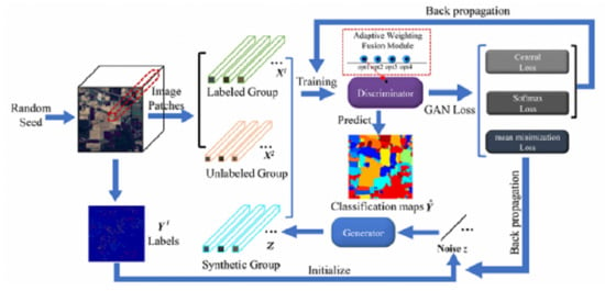
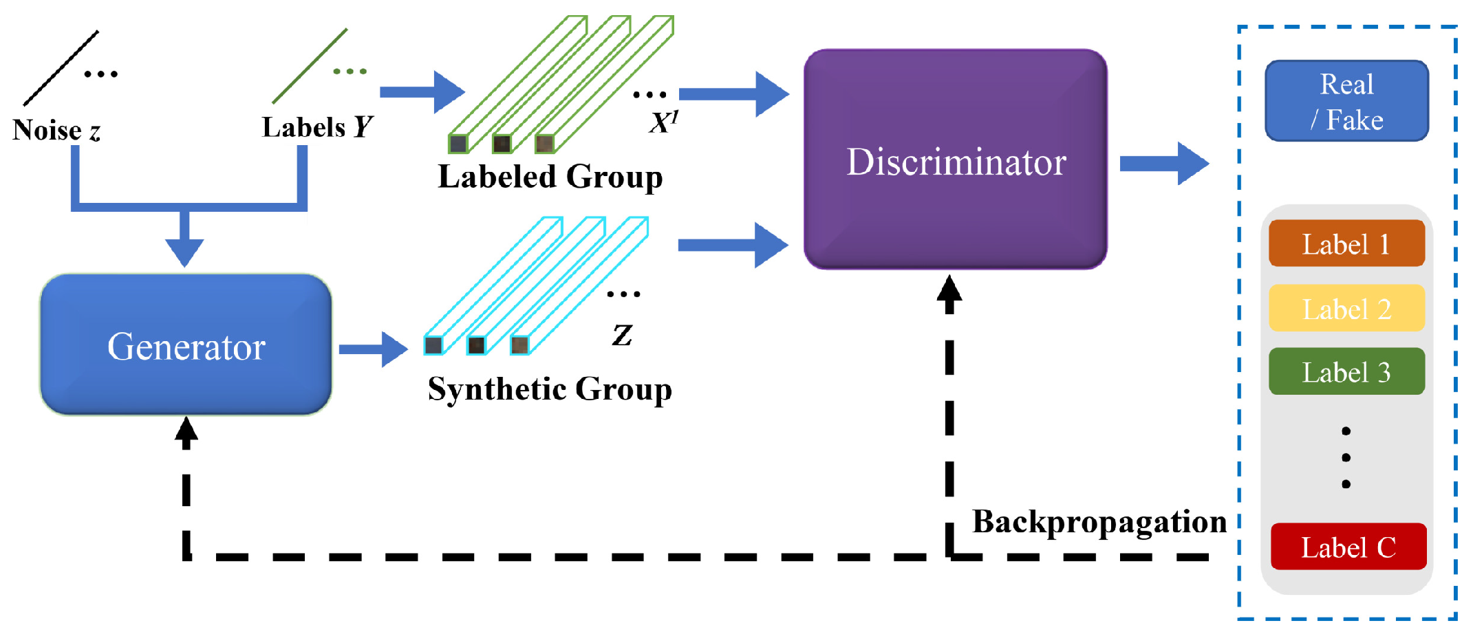
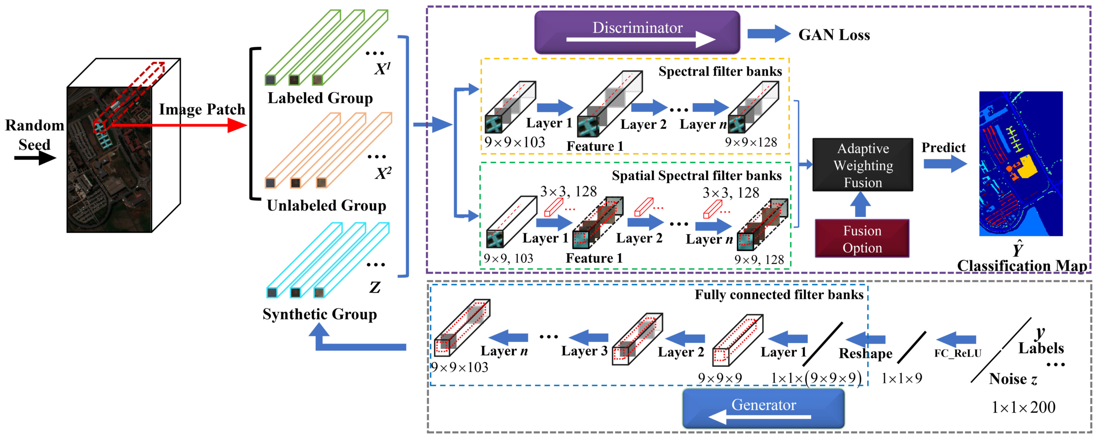
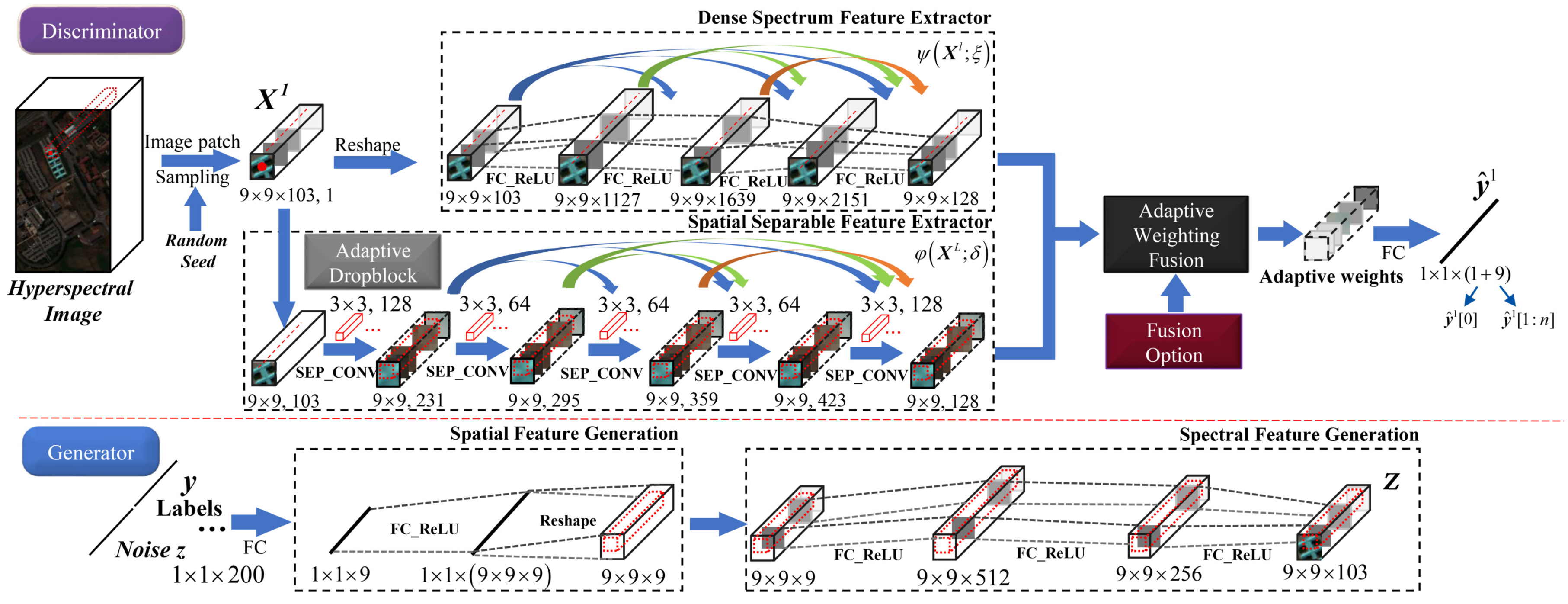
3.1. The Proposed AWF-GAN Framework
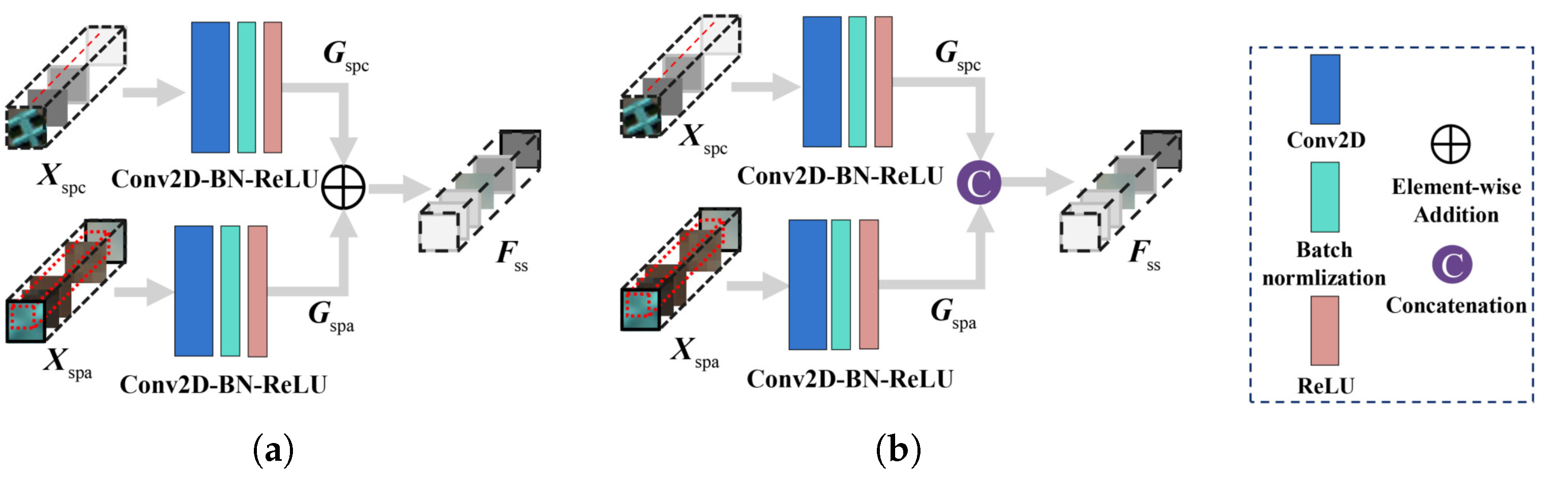
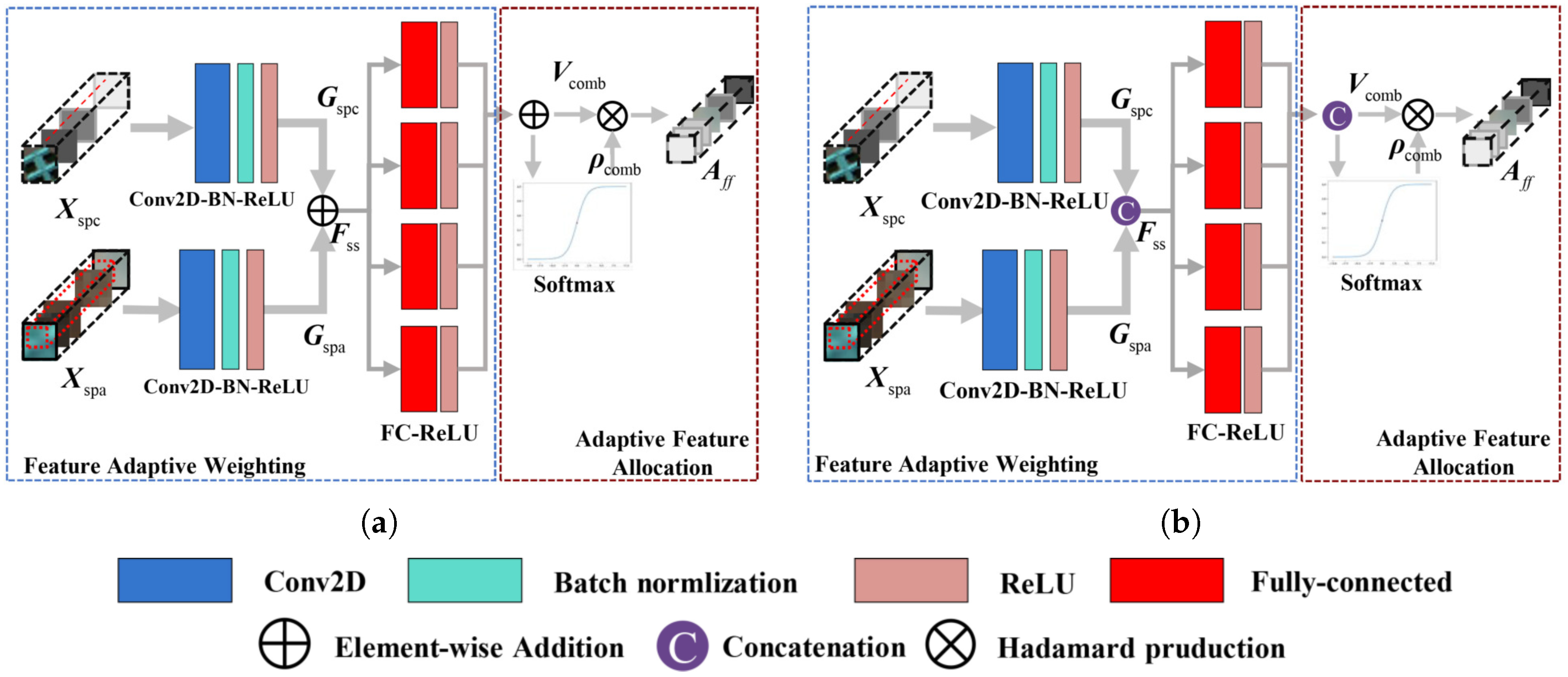
3.2. Adaptive Weighting Feature Fusion Module
3.2.1. Basic Feature Fusion Modules
3.2.2. Fusion Models with Adaptive Feature Weighting
3.3. Details of the AWF-GAN Architecture
3.3.1. Adaptive Weighting Feature Fusion Discriminator
3.3.2. Generator with Fully Connected Components
3.4. Training Loss Functions
4. Experimental Results
4.1. Experiment Setup
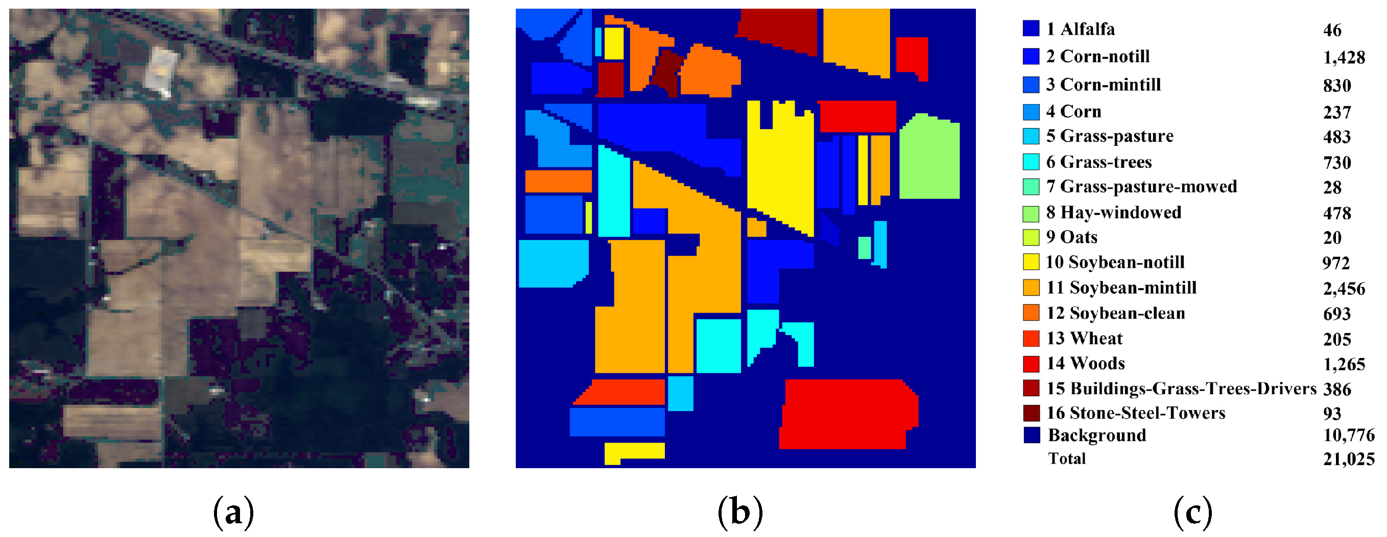
4.2. Experiments on the IN Dataset
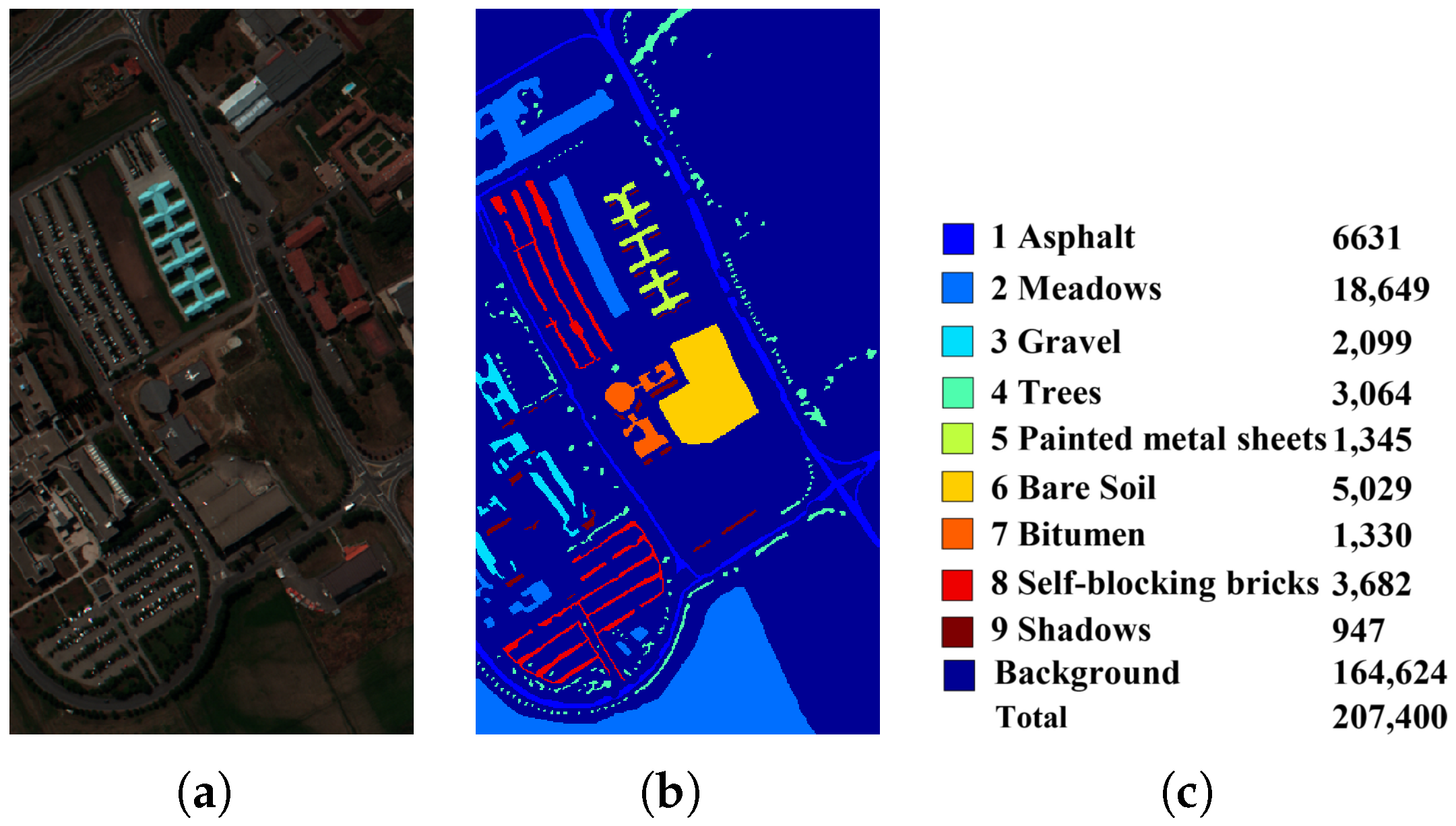
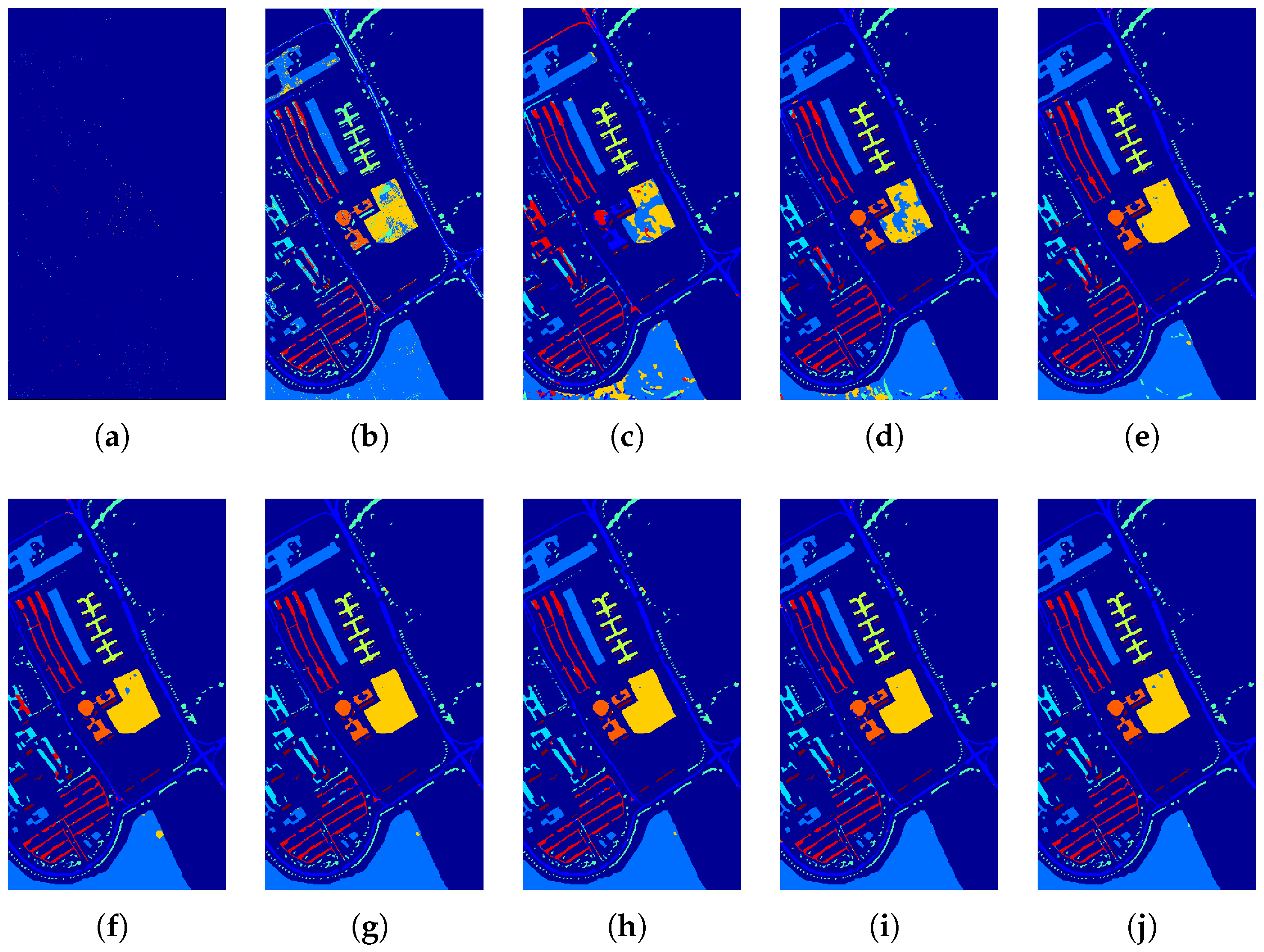
4.3. Experiments Using the UP Dataset
5. Discussion
5.1. Investigation of Running Time
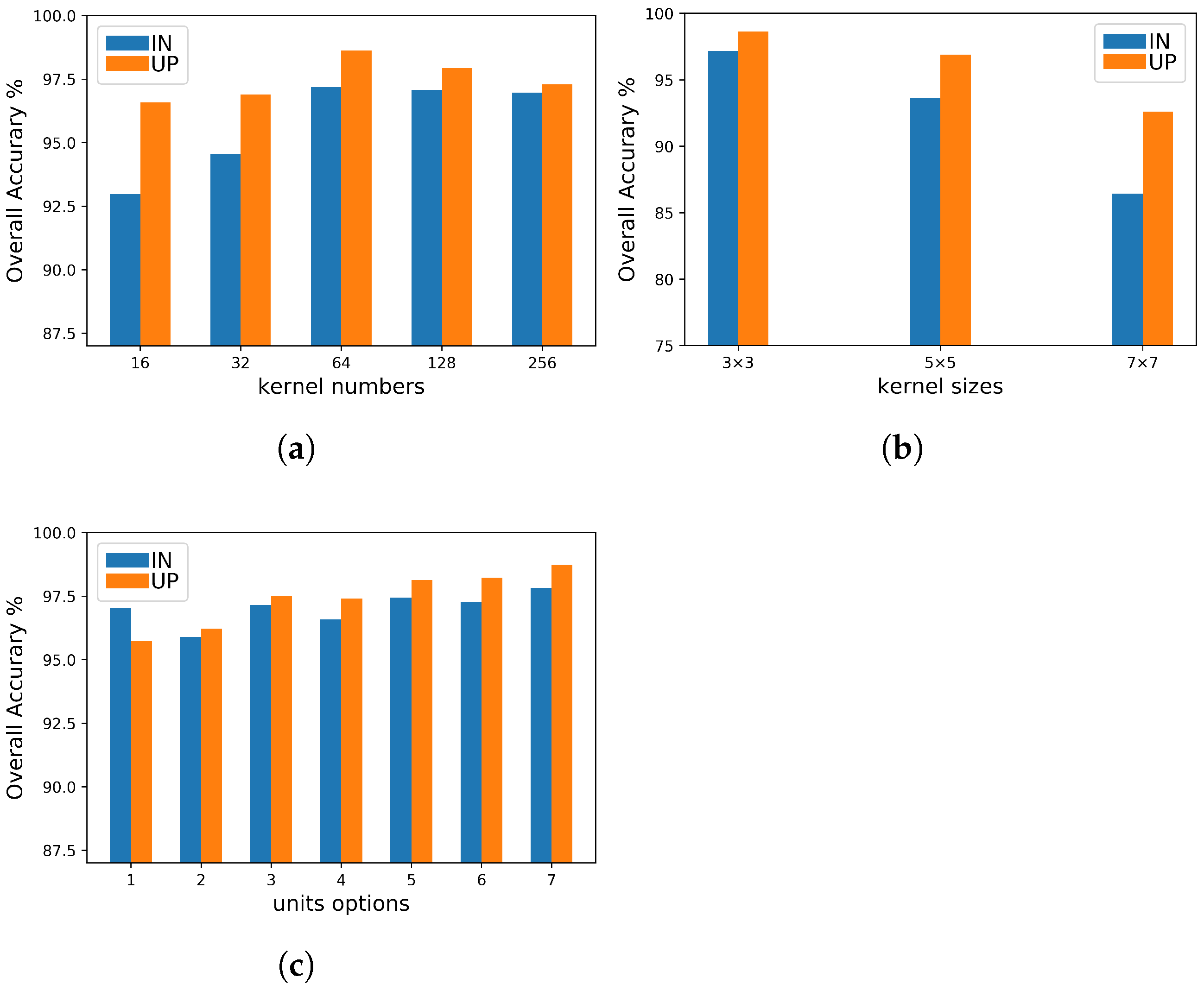
5.2. Kernel Setting and Units Selection for Feature Extraction
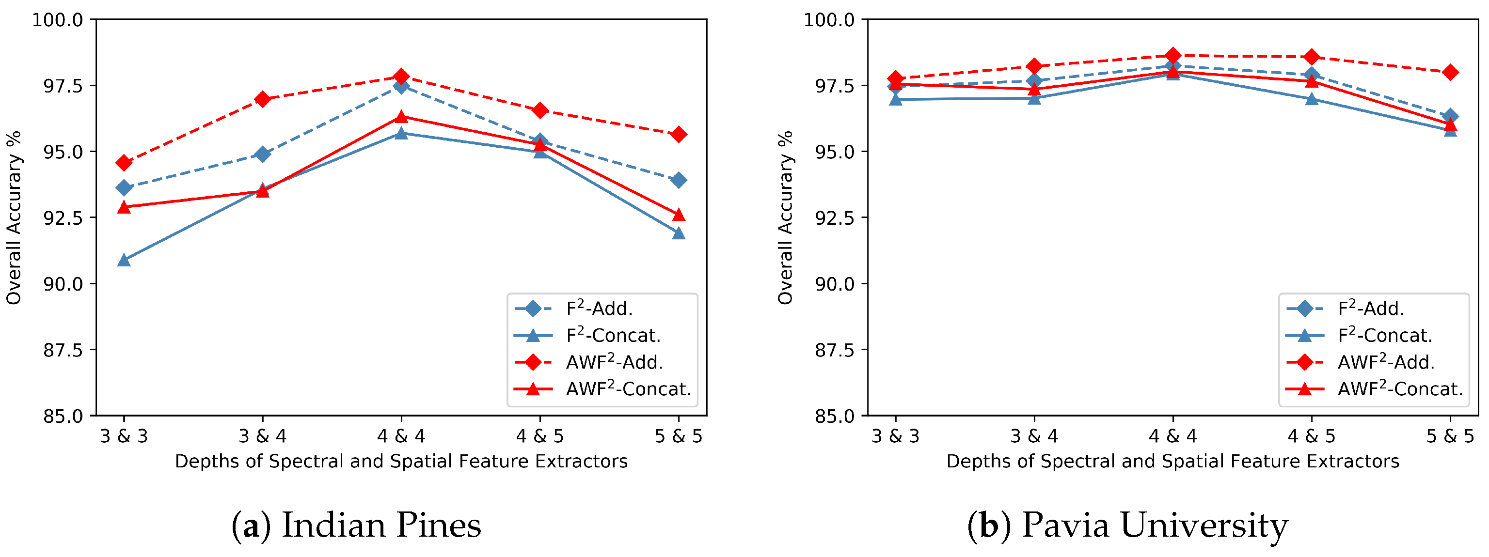
5.3. Depths of the Feature Extractors
5.4. Influence of Unlabeled Real HSI Cuboids for AWF-GANs
6. Conclusions
Author Contributions
Funding
Acknowledgments
Conflicts of Interest
References
- Berger, K.; Atzberger, C.; Danner, M.; D’Urso, G.; Mauser, W.; Vuolo, F.; Hank, T. Evaluation of the PROSAIL model capabilities for future hyperspectral model environments: A review study. Remote Sens. 2018, 10, 85. [Google Scholar] [CrossRef]
- Gerhards, M.; Schlerf, M.; Mallick, K.; Udelhoven, T. Challenges and future perspectives of multi-/Hyperspectral thermal infrared remote sensing for crop water-stress detection: A review. Remote Sens. 2019, 11, 1240. [Google Scholar] [CrossRef]
- Vali, A.; Comai, S.; Matteucci, M. Deep learning for land use and land cover classification based on hyperspectral and multispectral earth observation data: A review. Remote Sens. 2020, 12, 2495. [Google Scholar] [CrossRef]
- Chang, C.I.; Song, M.; Zhang, J.; Wu, C.C. Editorial for Special Issue “Hyperspectral Imaging and Applications”. Remote Sens. 2019, 11, 17. [Google Scholar] [CrossRef]
- Pullanagari, R.R.; Kereszturi, G.; Yule, I.J.; Ghamisi, P. Assessing the performance of multiple spectral–spatial features of a hyperspectral image for classification of urban land cover classes using support vector machines and artificial neural network. J. Appl. Remote Sens. 2017, 11, 026009. [Google Scholar] [CrossRef]
- Zhang, N.; Yang, G.; Pan, Y.; Yang, X.; Chen, L.; Zhao, C. A Review of Advanced Technologies and Development for Hyperspectral-Based Plant Disease Detection in the Past Three Decades. Remote Sens. 2020, 12, 3188. [Google Scholar] [CrossRef]
- Kycko, M.; Zagajewski, B.; Lavender, S.; Dabija, A. In situ hyperspectral remote sensing for monitoring of alpine trampled and recultivated species. Remote Sens. 2019, 11, 1296. [Google Scholar] [CrossRef]
- Ding, C.; Li, Y.; Xia, Y.; Wei, W.; Zhang, L.; Zhang, Y. Convolutional neural networks based hyperspectral image classification method with adaptive kernels. Remote Sens. 2017, 9, 618. [Google Scholar] [CrossRef]
- Luo, F.; Du, B.; Zhang, L.; Zhang, L.; Tao, D. Feature learning using spatial-spectral hypergraph discriminant analysis for hyperspectral image. IEEE Trans. Cybern. 2018, 49, 2406–2419. [Google Scholar] [CrossRef]
- Audebert, N.; Le Saux, B.; Lefèvre, S. Deep learning for classification of hyperspectral data: A comparative review. IEEE Geosci. Remote Sens. Mag. 2019, 7, 159–173. [Google Scholar] [CrossRef]
- Meng, Z.; Li, L.; Jiao, L.; Feng, Z.; Tang, X.; Liang, M. Fully Dense Multiscale Fusion Network for Hyperspectral Image Classification. Remote Sens. 2019, 11, 2718. [Google Scholar] [CrossRef]
- Shi, G.; Huang, H.; Liu, J.; Li, Z.; Wang, L. Spatial-Spectral Multiple Manifold Discriminant Analysis for Dimensionality Reduction of Hyperspectral Imagery. Remote Sens. 2019, 11, 2414. [Google Scholar] [CrossRef]
- Hu, W.; Huang, Y.; Wei, L.; Zhang, F.; Li, H. Deep convolutional neural networks for hyperspectral image classification. J. Sens. 2015, 2015, 333–344. [Google Scholar] [CrossRef]
- Chen, Y.; Jiang, H.; Li, C.; Jia, X.; Ghamisi, P. Deep feature extraction and classification of hyperspectral images based on convolutional neural networks. IEEE Trans. Geosci. Remote Sens. 2016, 54, 6232–6251. [Google Scholar] [CrossRef]
- Zhao, W.; Du, S. Spectral–spatial feature extraction for hyperspectral image classification: A dimension reduction and deep learning approach. IEEE Trans. Geosci. Remote Sens. 2016, 54, 4544–4554. [Google Scholar] [CrossRef]
- Mei, S.; Ji, J.; Hou, J.; Li, X.; Du, Q. Learning sensor-specific spatial-spectral features of hyperspectral images via convolutional neural networks. IEEE Trans. Geosci. Remote Sens. 2017, 55, 4520–4533. [Google Scholar] [CrossRef]
- Li, W.; Wu, G.; Zhang, F.; Du, Q. Hyperspectral image classification using deep pixel-pair features. IEEE Trans. Geosci. Remote Sens. 2016, 55, 844–853. [Google Scholar] [CrossRef]
- Imani, M.; Ghassemian, H. An overview on spectral and spatial information fusion for hyperspectral image classification: Current trends and challenges. Inf. Fusion 2020, 59, 59–83. [Google Scholar] [CrossRef]
- Li, Y.; Zhang, H.; Shen, Q. Spectral–spatial classification of hyperspectral imagery with 3D convolutional neural network. Remote Sens. 2017, 9, 67. [Google Scholar] [CrossRef]
- Zhang, M.; Li, W.; Du, Q. Diverse region-based CNN for hyperspectral image classification. IEEE Trans. Image Process. 2018, 27, 2623–2634. [Google Scholar] [CrossRef] [PubMed]
- Liang, M.; Jiao, L.; Meng, Z. A superpixel-based relational auto-encoder for feature extraction of hyperspectral images. Remote Sens. 2019, 11, 2454. [Google Scholar] [CrossRef]
- Liu, H.; Li, J.; He, L.; Wang, Y. Superpixel-guided layer-wise embedding CNN for remote sensing image classification. Remote Sens. 2019, 11, 174. [Google Scholar] [CrossRef]
- Zhong, Z.; Li, J.; Luo, Z.; Chapman, M. Spectral–spatial residual network for hyperspectral image classification: A 3-D deep learning framework. IEEE Trans. Geosci. Remote Sens. 2017, 56, 847–858. [Google Scholar] [CrossRef]
- Wang, W.; Dou, S.; Jiang, Z.; Sun, L. A fast dense spectral–spatial convolution network framework for hyperspectral images classification. Remote Sens. 2018, 10, 1068. [Google Scholar] [CrossRef]
- Zhu, K.; Chen, Y.; Ghamisi, P.; Jia, X.; Benediktsson, J.A. Deep convolutional capsule network for hyperspectral image spectral and spectral-spatial classification. Remote Sens. 2019, 11, 223. [Google Scholar] [CrossRef]
- Cui, X.; Zheng, K.; Gao, L.; Zhang, B.; Yang, D.; Ren, J. Multiscale spatial-spectral convolutional network with image-based framework for hyperspectral imagery classification. Remote Sens. 2019, 11, 2220. [Google Scholar] [CrossRef]
- Zhang, Y.; Huynh, C.P.; Ngan, K.N. Feature fusion with predictive weighting for spectral image classification and segmentation. IEEE Trans. Geosci. Remote Sens. 2019, 57, 6792–6807. [Google Scholar] [CrossRef]
- Lin, T.Y.; Dollár, P.; Girshick, R.; He, K.; Hariharan, B.; Belongie, S. Feature pyramid networks for object detection. In Proceedings of the CVPR 2017—2017 IEEE Conference on Computer Vision and Pattern Recognition, Honolulu, HI, USA, 22–25 July 2017; pp. 2117–2125. [Google Scholar]
- Mnih, V.; Kavukcuoglu, K.; Silver, D.; Rusu, A.A.; Veness, J.; Bellemare, M.G.; Graves, A.; Riedmiller, M.; Fidjeland, A.K.; Ostrovski, G.; et al. Human-level control through deep reinforcement learning. Nature 2015, 518, 529–533. [Google Scholar] [CrossRef]
- Fang, S.; Quan, D.; Wang, S.; Zhang, L.; Zhou, L. A Two-Branch Network with Semi-Supervised Learning for Hyperspectral Classification. In Proceedings of the IGARSS 2018—2018 IEEE International Geoscience and Remote Sensing Symposium, Valencia, Spain, 22–27 July 2018; pp. 3860–3863. [Google Scholar]
- Hu, Y.; An, R.; Wang, B.; Xing, F.; Ju, F. Shape Adaptive Neighborhood Information-Based Semi-Supervised Learning for Hyperspectral Image Classification. Remote Sens. 2020, 12, 2976. [Google Scholar] [CrossRef]
- Wan, S.; Gong, C.; Zhong, P.; Du, B.; Zhang, L.; Yang, J. Multiscale dynamic graph convolutional network for hyperspectral image classification. IEEE Trans. Geosci. Remote Sens. 2019, 58, 3162–3177. [Google Scholar] [CrossRef]
- Zhao, W.; Chen, X.; Chen, J.; Qu, Y. Sample Generation with Self-Attention Generative Adversarial Adaptation Network (SaGAAN) for Hyperspectral Image Classification. Remote Sens. 2020, 12, 843. [Google Scholar] [CrossRef]
- He, Z.; Liu, H.; Wang, Y.; Hu, J. Generative adversarial networks-based semi-supervised learning for hyperspectral image classification. Remote Sens. 2017, 9, 1042. [Google Scholar] [CrossRef]
- Zhan, Y.; Hu, D.; Wang, Y.; Yu, X. Semisupervised hyperspectral image classification based on generative adversarial networks. IEEE Geosci. Remote Sens. Lett. 2017, 15, 212–216. [Google Scholar] [CrossRef]
- Zhu, L.; Chen, Y.; Ghamisi, P.; Benediktsson, J.A. Generative adversarial networks for hyperspectral image classification. IEEE Trans. Geosci. Remote Sens. 2018, 56, 5046–5063. [Google Scholar] [CrossRef]
- Zhong, Z.; Li, J.; Clausi, D.A.; Wong, A. Generative adversarial networks and conditional random fields for hyperspectral image classification. IEEE Trans. Cybern. 2020, 50, 3318–3329. [Google Scholar] [CrossRef]
- Gao, H.; Yao, D.; Wang, M.; Li, C.; Liu, H.; Hua, Z.; Wang, J. A Hyperspectral Image Classification Method Based on Multi-Discriminator Generative Adversarial Networks. Sensors 2019, 19, 3269. [Google Scholar] [CrossRef]
- Feng, J.; Feng, X.; Chen, J.; Cao, X.; Zhang, X.; Jiao, L.; Yu, T. Generative adversarial networks based on collaborative learning and attention mechanism for hyperspectral image classification. Remote Sens. 2020, 12, 1149. [Google Scholar] [CrossRef]
- Wang, J.; Gao, F.; Dong, J.; Du, Q. Adaptive DropBlock-Enhanced Generative Adversarial Networks for Hyperspectral Image Classification. IEEE Trans. Geosci. Remote Sens. 2020, 1–14. [Google Scholar] [CrossRef]
- Radford, A.; Metz, L.; Chintala, S. Unsupervised representation learning with deep convolutional generative adversarial networks. In Proceedings of the International Conference on Learning Representations ICLR, Toulon, France, 20 January 2016; pp. 1–16. [Google Scholar]
- Feng, J.; Yu, H.; Wang, L.; Cao, X.; Zhang, X.; Jiao, L. Classification of hyperspectral images based on multiclass spatial–spectral generative adversarial networks. IEEE Trans. Geosci. Remote Sens. 2019, 57, 5329–5343. [Google Scholar] [CrossRef]
- Goodfellow, I.; Pouget-Abadie, J.; Mirza, M.; Xu, B.; Warde-Farley, D.; Ozair, S.; Courville, A.; Bengio, Y. Generative adversarial nets. Adv. Neural Inf. Process. Syst. 2014, 27, 2672–2680. [Google Scholar]
- Odena, A.; Olah, C.; Shlens, J. Conditional Image Synthesis With Auxiliary Classifier GANs. In International Conference on Machine Learning; PMLR: Sydney, Australia, 2017; pp. 2642–2651. [Google Scholar]
- Wen, Y.; Zhang, K.; Li, Z.; Qiao, Y. A discriminative feature learning approach for deep face recognition. In European Conference on Computer Vision; Springer: Amsterdam, The Netherlands, 2016; pp. 499–515. [Google Scholar]
- Cai, Y.; Dong, Z.; Cai, Z.; Liu, X.; Wang, G. Discriminative Spectral-Spatial Attention-Aware Residual Network for Hyperspectral Image Classification. In Proceedings of the 2019 10th Workshop on Hyperspectral Imaging and Signal Processing: Evolution in Remote Sensing (WHISPERS), Amsterdam, The Netherlands, 24–26 September 2019; pp. 1–5. [Google Scholar]
- Ioffe, S.; Szegedy, C. Batch normalization: Accelerating deep network training by reducing internal covariate shift. arXiv 2015, arXiv:1502.03167. [Google Scholar]
- He, K.; Zhang, X.; Ren, S.; Sun, J. Delving deep into rectifiers: Surpassing human-level performance on imagenet classification. In Proceedings of the IEEE International Conference on Computer Vision, Santiago, Chile, 13–16 December 2015; pp. 1026–1034. [Google Scholar]
- Marpu, P.R.; Pedergnana, M.; Dalla Mura, M.; Benediktsson, J.A.; Bruzzone, L. Automatic generation of standard deviation attribute profiles for spectral–spatial classification of remote sensing data. IEEE Geosci. Remote Sens. Lett. 2012, 10, 293–297. [Google Scholar] [CrossRef]


| Generator | ||||
|---|---|---|---|---|
| Block | Input Dimension | Layer/Operator | Reshape | Number of Neurons |
| Spatial Feature Generation | 1 × 1 × 200 | FC-ReLU | No | 9 |
| 1 × 1 × 9 | FC-ReLU | No | 9 × 9 × 9 | |
| 1 × 1 × (9 × 9 × 9) | † | Yes | † | |
| Spectral Feature Generation | 9 × 9 × 9 | FC-ReLU | No | 512 |
| 9 × 9 × 512 | FC-ReLU | No | 256 | |
| 9 × 9 × 256 | FC-ReLU | No | 103 | |
| Synthetic HSI cuboid Z | 9 × 9 × 103 | Output | † | † |
| Discriminator D | |||||
|---|---|---|---|---|---|
| Compoment | Input Dimension | Layer /Operator | Neural Units | Kernel | Concatenation |
| Dense Spectrum Feature Extractor | 9 × 9 × 103 | FC-ReLU | 1024 | † | No |
| 9 × 9 × 1127 | FC-ReLU | 512 | † | Yes | |
| 9 × 9 × 1639 | FC-ReLU | 512 | † | Yes | |
| 9 × 9 × 2151 | FC-ReLU | 128 | † | No | |
| Spectral Feature | 9 × 9 × 128 | Output | † | † | † |
| Spatially Separable Feature Extractor | 9 × 9 × 103 | Adaptive Dropblock | † | † | No |
| 9 × 9 × 103 | Sep-CONV | † | 3 × 3 × 128 | No | |
| 9 × 9 × 231 | Sep-CONV | † | 3 × 3 × 64 | Yes | |
| 9 × 9 × 295 | Sep-CONV | † | 3 × 3 × 64 | Yes | |
| 9 × 9 × 359 | Sep-CONV | † | 3 × 3 × 64 | Yes | |
| 9 × 9 × 423 | Sep-CONV | † | 3 × 3 × 128 | No | |
| Spatial Feature | 9 × 9 × 128 | Output | † | † | † |
| Adaptive Weight Matrix | / | Adaptive Weighting Feature Fusion | † | † | † |
| Classification Vectors | 1 × 1 × (1 + 9) | Fully-connection | † | † | † |
| Class | Train (Test) | SVM | HS-GAN | 3D-GAN | SS-GAN | AD-GAN | AWF-GANs | |||
|---|---|---|---|---|---|---|---|---|---|---|
| F-Con. | F-Add. | AWF-Con. | AWF-Add. | |||||||
| 1 | 5 (41) | 64.49 ± 0.81 | 20.39 ± 7.35 | 58.48 ± 0.26 | 93.04 ± 0.99 | 100 ± 0.00 | 100 ± 0.00 | 100 ± 0.00 | 100 ± 0.00 | 100 ± 0.00 |
| 2 | 72 (1356) | 81.06 ± 3.04 | 68.29 ± 0.75 | 90.49 ± 0.57 | 96.1 ± 0.32 | 96.24 ± 0.27 | 96.95 ± 0.16 | 95.53 ± 0.19 | 95.97 ± 0.09 | 98.00 ± 0.09 |
| 3 | 42 (788) | 73.55 ± 0.98 | 62.25 ± 1.79 | 81.14 ± 0.90 | 92.72 ± 0.39 | 93.45 ± 0.81 | 97.03 ± 0.06 | 93.71 ± 0.09 | 95.07 ± 0.10 | 95.14 ± 0.14 |
| 4 | 12 (225) | 40.02 ± 0.13 | 60.45 ± 3.57 | 90.72 ± 0.87 | 92.51 ± 0.59 | 94.09 ± 0.15 | 92.81 ± 0.30 | 100 ± 0.00 | 98.75 ± 0.18 | 98.84 ± 0.25 |
| 5 | 25 (458) | 81.79 ± 0.50 | 72.34 ± 7.89 | 72.34 ± 0.07 | 99.07 ± 0.79 | 99.44 ± 0.18 | 94.02 ± 0.09 | 99.16 ± 0.13 | 99.45 ± 0.25 | 100 ± 0.00 |
| 6 | 37 (693) | 87.88 ± 0.41 | 90.78 ± 1.06 | 90.78 ± 1.06 | 98.95 ± 0.74 | 99.75 ± 0.24 | 96.31 ± 0.13 | 99.34 ± 0.14 | 95.97 ± 0.08 | 98.56 ± 0.81 |
| 7 | 3 (25) | 59.13 ± 0.18 | 34.79 ± 5.75 | 94.56 ± 0.67 | 96.27 ± 0.83 | 100 ± 0.00 | 78.51 ± 0.30 | 100 ± 0.00 | 80.09 ± 0.34 | 100 ± 0.00 |
| 8 | 24 (454) | 91.13 ± 0.30 | 94.56 ± 1.67 | 99.09 ± 0.14 | 99.58 ± 0.60 | 99.76 ± 0.00 | 98.89 ± 0.27 | 99.73 ± 0.22 | 98.95 ± 0.11 | 100 ± 0.00 |
| 9 | 3 (18) | 40.00 ± 0.25 | 34.63 ± 3.85 | 34.63 ± 0.38 | 98.09 ± 0.57 | 100 ± 0.00 | 66.53 ± 1.53 | 84.35 ± 0.30 | 79.77 ± 0.63 | 100 ± 0.00 |
| 10 | 49 (923) | 78.76 ± 2.08 | 55.85 ± 10.4 | 93.60 ± 0.25 | 93.05 ± 0.32 | 92.58 ± 1.32 | 91.49 ± 0.32 | 98.03 ± 0.18 | 93.89 ± 0.25 | 96.98 ± 0.16 |
| 11 | 123 (2332) | 93.59 ± 1.91 | 75.99 ± 1.46 | 91.30 ± 0.21 | 94.68 ± 0.43 | 96.52 ± 0.26 | 94.46 ± 0.21 | 97.89 ± 0.56 | 96.07 ± 0.29 | 97.71 ± 0.27 |
| 12 | 30 (563) | 72.61 ± 0.76 | 50.89 ± 1.46 | 75.99 ± 0.14 | 91.41 ± 0.88 | 97.80 ± 0.62 | 89.94 ± 0.34 | 95.85 ± 0.15 | 96.40 ± 0.37 | 98.65 ± 0.20 |
| 13 | 11 (194) | 78.34 ± 0.13 | 82.27 ± 1.06 | 82.27 ± 1.06 | 98.80 ± 1.53 | 100 ± 0.00 | 97.32 ± 0.22 | 100 ± 0.00 | 98.94 ± 0.16 | 100 ± 0.00 |
| 14 | 64 (1201) | 92.42 ± 0.39 | 93.26 ± 1.30 | 90.89 ± 0.13 | 98.37 ± 1.58 | 98.26 ± 0.33 | 98.66 ± 0.37 | 99.03 ± 0.13 | 98.62 ± 0.38 | 98.35 ± 0.05 |
| 15 | 20 (366) | 62.08 ± 0.13 | 45.75 ± 1.35 | 90.95 ± 0.13 | 94.35 ± 0.37 | 97.65 ± 0.24 | 89.54 ± 0.43 | 97.45 ± 0.15 | 92.81 ± 0.29 | 96.39 ± 0.31 |
| 16 | 5 (88) | 28.43 ± 1.36 | 79.89 ± 0.81 | 85.05 ± 0.74 | 96.96 ± 2.5 | 95.08 ± 1.09 | 81.27 ± 0.53 | 88.82 ± 0.38 | 89.46 ± 0.59 | 92.99 ± 0.07 |
| OA(%) | 82.86 ± 1.43 | 77.89 ± 1.62 | 92.28 ± 3.05 | 95.35 ± 0.14 | 96.72 ± 0.17 | 94.90 ± 0.14 | 97.45 ± 0.27 | 96.32 ± 0.17 | 97.83 ± 0.11 | |
| AA(%) | 70.37 ± 2.72 | 63.94 ± 2.77 | 82.60 ± 4.79 | 95.87 ± 0.16 | 97.54 ± 0.21 | 91.56 ± 0.39 | 96.81 ± 0.06 | 94.47 ± 0.20 | 98.30 ± 0.18 | |
| 80.12 ± 1.77 | 75.56 ± 0.89 | 90.51 ± 0.35 | 94.69 ± 0.16 | 96.26 ± 0.20 | 94.10 ± 0.10 | 97.09 ± 0.09 | 95.8 ± 0.28 | 97.53 ± 0.09 | ||
| Sample | Classification Method | ||||||||
|---|---|---|---|---|---|---|---|---|---|
| (Per Class) | SVM | HS-GAN | 3D-GAN | SS-GAN | AD-GAN | AWF2-GANs | |||
| F-Con. | F-Add. | AWF-Con. | AWF-Add. | ||||||
| 110 (1%) | 60.38 ± 1.60 | 59.28 ± 1.47 | 69.79 ± 0.76 | 72.81 ± 0.62 | 75.84 ± 0.55 | 77.59 ± 0.47 | 80.17 ± 0.39 | 80.75 ± 0.35 | 83.77 ± 0.23 |
| 314 (3%) | 72.59 ± 1.33 | 71.87 ± 1.35 | 83.40 ± 0.57 | 85.57 ± 0.67 | 87.67 ± 0.53 | 92.47 ± 0.64 | 95.73 ± 0.42 | 93.85 ± 0.44 | 95.32 ± 0.17 |
| 520 (5%) | 81.70 ± 1.39 | 76.67 ± 1.44 | 91.71 ± 0.67 | 94.46 ± 0.46 | 95.89 ± 0.39 | 94.49 ± 0.0.57 | 96.82 ± 0.28 | 95.79 ± 0.34 | 97.53 ± 0.21 |
| 726 (7%) | 84.77 ± 1.28 | 78.89 ± 1.16 | 93.24 ± 0.44 | 95.77 ± 0.52 | 96.77 ± 0.48 | 96.30 ± 0.31 | 97.83 ± 0.33 | 97.21 ± 0.30 | 98.16 ± 0.25 |
| 1031 (10%) | 88.90 ± 1.01 | 83.40 ± 1.20 | 95.79 ± 0.21 | 97.79 ± 0.13 | 97.56 ± 0.18 | 97.33 ± 0.14 | 98.70 ± 0.12 | 98.57 ± 0.22 | 99.07 ± 0.04 |
| Class | Train (Test) | SVM | HS-GAN | 3D-GAN | SS-GAN | AD-GAN | AWF-GANs | |||
|---|---|---|---|---|---|---|---|---|---|---|
| F-Con. | F-Add. | AWF-Con. | AWF-Add. | |||||||
| 1 | 54 (6577) | 84.53 ± 2.38 | 75.46 ± 1.53 | 96.73 ± 0.49 | 98.97 ± 0.14 | 98.65 ± 0.15 | 96.75 ± 0.29 | 96.80 ± 0.01 | 97.70 ± 0.19 | 100 ± 0.00 |
| 2 | 150 (18499) | 95.48 ± 1.67 | 93.57 ± 0.86 | 97.82 ± 0.39 | 99.33 ± 0.03 | 98.96 ± 0.35 | 98.85 ± 0.30 | 98.94 ± 0.07 | 98.89 ± 0.13 | 98.57 ± 0.38 |
| 3 | 17 (2082) | 67.50 ± 0.83 | 82.24 ± 4.23 | 95.00 ± 0.64 | 86.40 ± 0.15 | 98.69 ± 0.03 | 93.82 ± 0.19 | 97.68 ± 0.18 | 90.89 ± 0.25 | 99.37 ± 0.61 |
| 4 | 25 (3039) | 95.33 ± 0.10 | 85.64 ± 1.13 | 98.87 ± 0.59 | 99.47 ± 0.10 | 99.91 ± 0.05 | 98.00 ± 0.14 | 96.68 ± 0.19 | 97.93 ± 0.51 | 96.48 ± 0.38 |
| 5 | 14 (1331) | 51.86 ± 0.14 | 78.98 ± 5.26 | 1.00 ± 0.00 | 99.54 ± 0.08 | 99.92 ± 0.02 | 98.81 ± 0.24 | 99.68 ± 0.37 | 99.73 ± 0.30 | 100 ± 0.00 |
| 6 | 41 (4988) | 75.47 ± 0.05 | 70.07 ± 0.72 | 97.09 ± 0.46 | 97.51 ± 0.19 | 97.79 ± 0.22 | 98.49 ± 0.26 | 99.02 ± 0.13 | 99.05 ± 0.14 | 99.80 ± 0.30 |
| 7 | 11 (1319) | 80.90 ± 0.61 | 77.67 ± 2.99 | 95.95 ± 0.64 | 95.96 ± 0.45 | 95.63 ± 0.06 | 100 ± 0.00 | 100 ± 0.00 | 97.10 ± 0.38 | 100 ± 0.00 |
| 8 | 30 (3652) | 84.19 ± 0.34 | 80.98 ± 0.27 | 89.98 ± 0.96 | 91.73 ± 0.36 | 85.09 ± 0.43 | 94.84 ± 0.18 | 95.98 ± 0.14 | 96.00 ± 0.22 | 97.39 ± 0.25 |
| 9 | 8 (939) | 50.85 ± 0.11 | 90.96 ± 0.38 | 97.78 ± 0.41 | 99.85 ± 0.02 | 100 ± 0.00 | 100 ± 0.00 | 100 ± 0.00 | 99.85 ± 0.12 | 98.62 ± 0.47 |
| OA(%) | 86.26 ± 1.19 | 84.98 ± 2.33 | 97.07 ± 0.19 | 97.25 ± 0.15 | 97.39 ± 0.09 | 98.05 ± 0.24 | 98.24 ± 0.16 | 98.01 ± 0.19 | 98.68 ± 0.22 | |
| AA(%) | 76.23 ± 2.75 | 81.11 ± 1.21 | 96.99 ± 0.36 | 96.53 ± 0.13 | 97.18 ± 0.07 | 97.68 ± 0.32 | 98.53 ± 0.11 | 97.43 ± 0.20 | 98.81 ± 0.20 | |
| 81.76 ± 1.54 | 80.56 ± 1.77 | 96.49 ± 0.46 | 96.37 ± 0.19 | 96.53 ± 0.12 | 97.31 ± 0.26 | 97.66 ± 0.27 | 97.47 ± 0.18 | 98.12 ± 0.43 | ||
| Sample | Classification Method | ||||||||
|---|---|---|---|---|---|---|---|---|---|
| Per Class | SVM | HS-GAN | 3D-GAN | SS-GAN | AD-GAN | AWF-GANs | |||
| F-Con. | F-Add. | AWF-Con. | AWF-Add. | ||||||
| 48 (0.1%) | 67.75 ± 1.54 | 66.96 ± 1.23 | 80.12 ± 0.98 | 81.73 ± 1.01 | 83.38 ± 0.95 | 85.75 ± 1.12 | 87.00 ± 0.97 | 89.76 ± 0.89 | 90.74 ± 0.92 |
| 91 (0.2%) | 78.33 ± 1.34 | 75.57 ± 1.19 | 89.57 ± 1.03 | 89.98 ± 0.97 | 91.09 ± 0.89 | 91.54 ± 0.98 | 91.97 ± 0.88 | 93.85 ± 1.16 | 94.80 ± 0.77 |
| 176 (0.4%) | 82.69 ± 1.11 | 78.87 ± 1.36 | 93.13 ± 0.88 | 94.57 ± 0.82 | 95.38 ± 1.06 | 95.35 ± 0.61 | 96.20 ± 0.45 | 96.54 ± 0.54 | 97.31 ± 0.37 |
| 347 (0.8%) | 86.26 ± 0.97 | 84.98 ± 1.29 | 97.07 ± 0.75 | 97.25 ± 0.79 | 97.39 ± 0.61 | 96.90 ± 0.77 | 97.31 ± 0.48 | 98.01 ± 0.32 | 98.68 ± 0.29 |
| 432 (1%) | 88.74 ± 1.26 | 86.99 ± 0.97 | 97.26 ± 0.65 | 97.47 ± 0.16 | 97.64 ± 0.22 | 97.97 ± 0.13 | 98.09 ± 0.21 | 98.26 ± 0.16 | 98.73 ± 0.09 |
| Methods | Training Time (s) | Testing Time (s) | ||
|---|---|---|---|---|
| IndianPines | Pavia University | IndianPines | Pavia University | |
| SVM | 1.21 ± 1.05 | 1.05 ± 0.95 | 1.11 ± 0.19 | 1.2 ± 0.23 |
| HS-GAN | 465.35 ± 34.54 | 586.77 ± 25.35 | 0.37 ± 0.05 | 0.55 ± 0.11 |
| 3D-GAN | 1047.62 ± 70.29 | 798.22 ± 34.46 | 0.97 ± 0.15 | 2.35 ± 0.23 |
| SS-GAN | 770.89 ± 75.55 | 535.79 ± 59.66 | 8.36 ± 0.19 | 16.44 ± 0.07 |
| AD-GAN | 574.24 ± 66.75 | 409.26 ± 50.99 | 5.79 ± 0.22 | 6.76 ± 0.12 |
| F-Con. | 187.02 ± 10.16 | 165.56 ± 8.52 | 5.23 ± 0.10 | 4.83 ± 0.31 |
| F-Add. | 112.53 ± 11.59 | 99.68 ± 7.93 | 2.16 ± 0.14 | 4.91 ± 0.07 |
| AWF-Con. | 185.68 ± 32.67 | 138.59 ± 21.89 | 5.23 ± 0.09 | 10.58 ± 0.05 |
| AWF-Add. | 140.99 ± 25.78 | 118.365 ± 17.87 | 3.31 ± 0.12 | 7.22 ± 0.08 |
| Dataset | Models | 0 | 300 | 1000 | 5000 |
|---|---|---|---|---|---|
| Indian Pines | HS-GAN | 65.89 | 65.38 | 60.16 | 59.86 |
| SS-GAN | 89.69 | 91.28 | 88.22 | 79.85 | |
| F-Con. | 94.79 | 93.07 | 89.73 | 67.49 | |
| F-Add. | 95.95 | 96.60 | 94.83 | 96.47 | |
| AWF-Con. | 93.86 | 94.83 | 95.32 | 79.82 | |
| AWF-Add. | 96.06 | 96.47 | 95.16 | 78.57 | |
| Pavia University | HS-GAN | 83.42 | 83.69 | 80.87 | 78.89 |
| SS-GAN | 96.64 | 96.75 | 94.82 | 92.80 | |
| F-Con. | 98.02 | 97.99 | 95.66 | 84.35 | |
| F-Add. | 98.03 | 98.27 | 94.46 | 82.17 | |
| AWF-Con. | 97.91 | 98.01 | 93.39 | 90.59 | |
| AWF-Add. | 98.16 | 98.37 | 96.69 | 91.26 |
Publisher’s Note: MDPI stays neutral with regard to jurisdictional claims in published maps and institutional affiliations. |
© 2021 by the authors. Licensee MDPI, Basel, Switzerland. This article is an open access article distributed under the terms and conditions of the Creative Commons Attribution (CC BY) license (http://creativecommons.org/licenses/by/4.0/).
Share and Cite
Liang, H.; Bao, W.; Shen, X. Adaptive Weighting Feature Fusion Approach Based on Generative Adversarial Network for Hyperspectral Image Classification. Remote Sens. 2021, 13, 198. https://doi.org/10.3390/rs13020198
Liang H, Bao W, Shen X. Adaptive Weighting Feature Fusion Approach Based on Generative Adversarial Network for Hyperspectral Image Classification. Remote Sensing. 2021; 13(2):198. https://doi.org/10.3390/rs13020198
Chicago/Turabian StyleLiang, Hongbo, Wenxing Bao, and Xiangfei Shen. 2021. "Adaptive Weighting Feature Fusion Approach Based on Generative Adversarial Network for Hyperspectral Image Classification" Remote Sensing 13, no. 2: 198. https://doi.org/10.3390/rs13020198
APA StyleLiang, H., Bao, W., & Shen, X. (2021). Adaptive Weighting Feature Fusion Approach Based on Generative Adversarial Network for Hyperspectral Image Classification. Remote Sensing, 13(2), 198. https://doi.org/10.3390/rs13020198