HRCNet: High-Resolution Context Extraction Network for Semantic Segmentation of Remote Sensing Images

Abstract

Semantic segmentation is a significant method in remote sensing image (RSIs) processing and has been widely used in various applications. Conventional convolutional neural network (CNN)-based semantic segmentation methods are likely to lose the spatial information in the feature extraction stage and usually pay little attention to global context information. Moreover, the imbalance of category scale and uncertain boundary information meanwhile exists in RSIs, which also brings a challenging problem to the semantic segmentation task. To overcome these problems, a high-resolution context extraction network (HRCNet) based on a high-resolution network (HRNet) is proposed in this paper. In this approach, the HRNet structure is adopted to keep the spatial information. Moreover, the light-weight dual attention (LDA) module is designed to obtain global context information in the feature extraction stage and the feature enhancement feature pyramid (FEFP) structure is promoted and employed to fuse the contextual information of different scales. In addition, to achieve the boundary information, we design the boundary aware (BA) module combined with the boundary aware loss (BAloss) function. The experimental results evaluated on Potsdam and Vaihingen datasets show that the proposed approach can significantly improve the boundary and segmentation performance up to 92.0% and 92.3% on overall accuracy scores, respectively. As a consequence, it is envisaged that the proposed HRCNet model will be an advantage in remote sensing images segmentation.

1. Introduction

Remote sensing images (RSIs) collected from satellite and aerial platforms are widely used in various applications, such as land-use mapping, urban resources management, and disaster monitoring [1]. Deep learning based segmentation methods composing of instance segmentation and semantic segmentation, which are crucial for automatic analysis and exploitation of the RSIs in the aforementioned applications. Instance segmentation methods are originated from the region-based CNN (RCNN [2,3,4,5]). These methods focus on region classification with less consideration of the background, which are especially suit for the region highlight field, such as ice-wedge detection [6,7,8,9]. However, for urban scenes, each component needs to be concerned, so semantic segmentation would be a better choice. Due to the rapid development of remote sensing technology, especially the improvement of customized imaging sensors, a massive number of high-quality images are available to be analysed [10]. The ever-increasing RSIs can facilitate massive semantic segmentation methods being applied in satellite remote sensing images analysis.

The remote sensing images segmentation performance is determined by three vital factors: spatial information, global context information and boundary details. First, spatial information of RSIs is beneficial in restoring damaged structure and reducing the effects brought by cutting operation, since image is cut into pieces resulting in the destruction of the structure before the segmentation operation. Second, global context information should be employed to help search for the categories relevance in images as categories are difficult to be discriminated by only making use of the local information. Third, boundary of the objects is often blurred leading to a degrading classification performance due to the satellite movement. Therefore, the aforementioned three factors should be considered before the network potentials being realized.

Encoder-decoder based convolutional neural networks (CNNs) and its variants (e.g., SegNet, U-Net) led to a breakthrough of semantic segmentation in remote sensing images (RSIs) because of the concern on spatial information [11,12]. But, this so-called “encoder-decoder” structure has the limited ability to rebuild the spatial information and pays little attention to the boundary. To solve this problem, Sun et al. [13] introduced a parallel-branch network called High-Resolution Network (HRNet) to combine high-resolution features (mainly include structural information, such as the shape) and high-level semantic information (could be described as the logical description, such as the category information) in the “decoder”, instead of fusing the shallow layers with less semantic information, which yields an improvement in spatial information for objects segmentation. However, such a method has no ability to use global context information so that the performance of recognition on objects and regions is impaired [1]. Consequently, spatial attention mechanism is proposed for achieving image contextual information by building the relationship between local pixel and global pixels [14]. This attention mechanism makes the CNNs context-aware, especially promoting the classification accuracy of large targets [15], but results in high computation load and great redundant information along with the promotion [16]. Meanwhile, the high-resolution multiple branches also enlarge the size of HRNet, making this network heavy-weight. In addition, with respect to boundary details, HRNet can make the boundary more clear to be better recognized, but still far away from the groundtruth.

According to the previous work, UNet has the limited ability to obtain the spatial information, HRNet is capable of fusing enough spatial information whereas the further research on contextual information and boundary information is less considered. Therefore, on the basis of HRNet backbone, a novel architecture called High-Resolution Context Extraction Network (HRCNet, see Figure 1) is proposed to make the attention mechanism light-weight to effectively acquire global context information and helps the boundary being well recognized. First, based on Fu’s work [17], the light-weight dual attention (LDA) module is designed with high performance of feature optimization and less computation load. Second, Feature Enhancement Feature Pyramid (FEFP) module is presented to merge multi-scale information to cope with the scale inconsistency problem. Finally, Boundary Aware (BA) module is introduced to make the network focus on the boundary. In addition, considering that semantic segmentation only focuses on pixel-level classification, it lacks region-level and image-level optimization [18,19]. To this end, we propose the multi-level loss functions composing of cross entropy loss (CEloss [20]), boundary aware loss (BAloss [21]) and semantic encoding loss (SEloss [22]) to supervise the training procedure, making the model focus on pixel-level classification, region-level (boundary) classification, and image-level classification at the same time [21]. The proposed model is compared with other methods on International Society for Photogrammetry and Remote Sensing (ISPRS) 2D semantic labeling benchmark and achieves the best (92.0% and 92.3% overall accuracy scores on Potsdam and Vaihingen datasets, respectively). The remainder of this paper is organized as follows. Section 2 introduces some related work. Section 3 demonstrates the overall structure of our proposed model and the details of each module. Section 4 presents the experimental results and details. Section 5 shows the discussions and limitations. Section 6 concludes this study.

To be more clear, the main contributions of this work are summarized as follows:

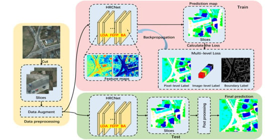
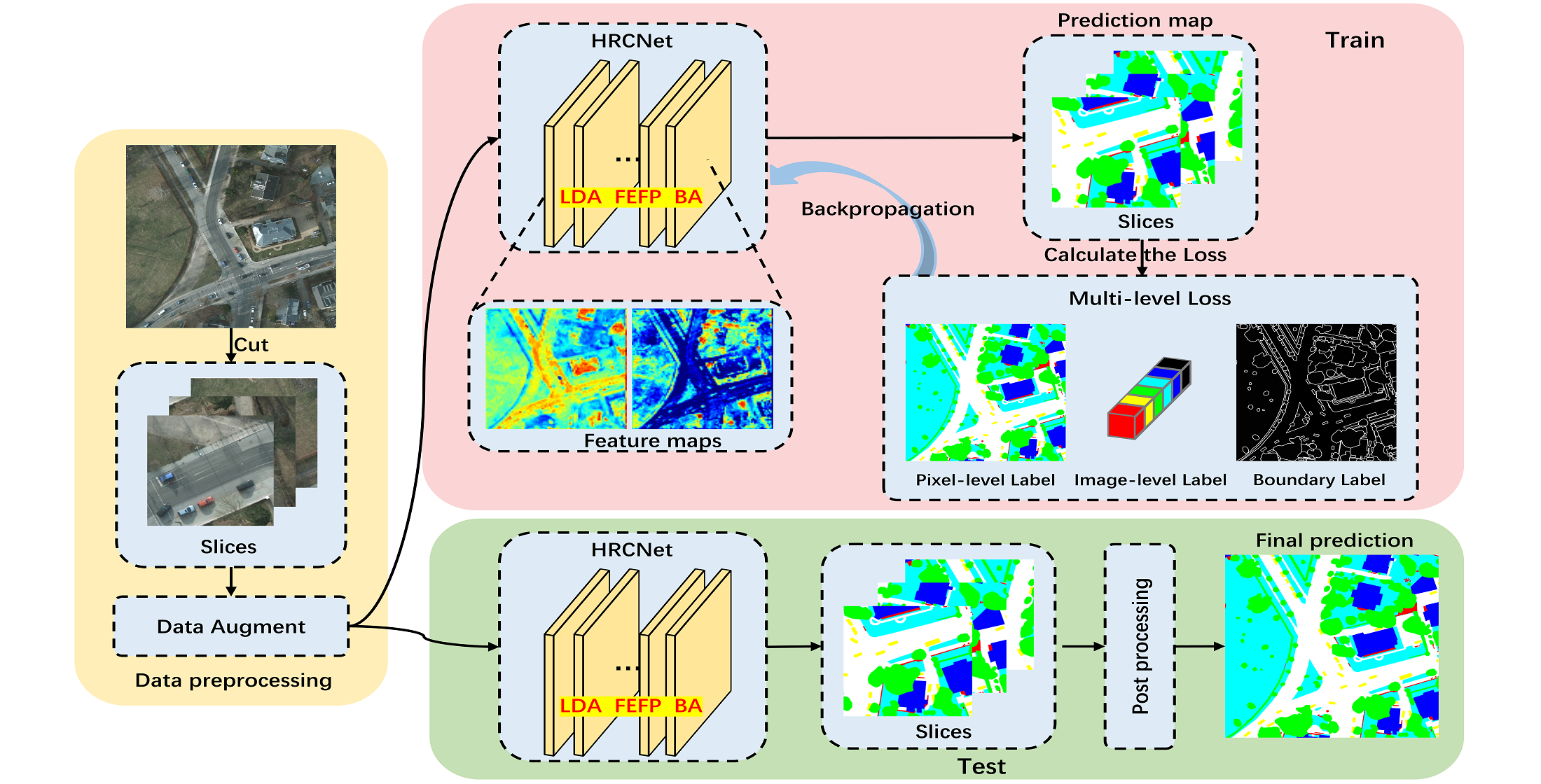
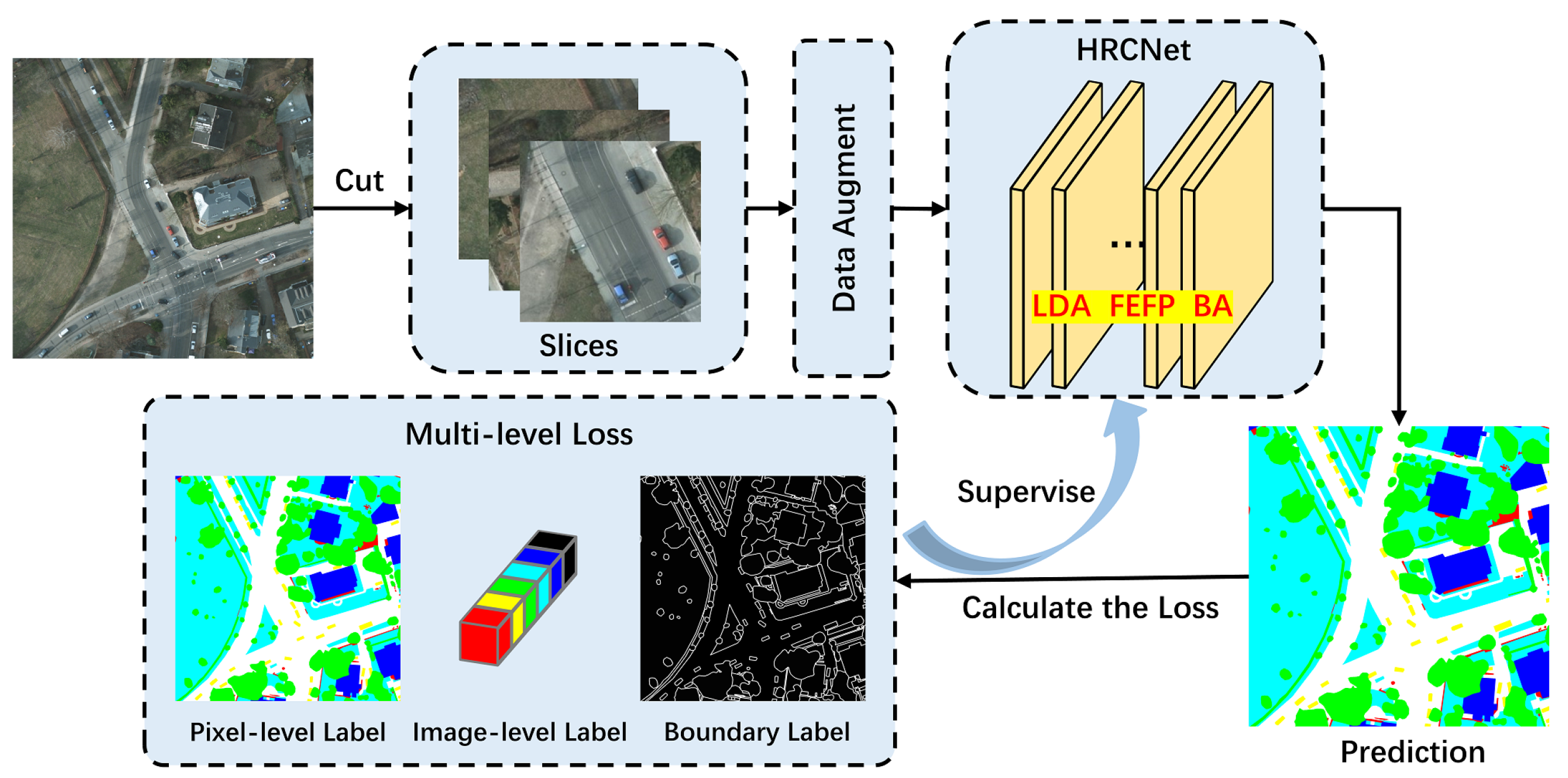
• Combining the light-weight dual attention (LDA) mechanism and boundary aware (BA) module, we propose a light-weight high-resolution context extraction network (HRCNet) to obtain global context information and improve the boundary.
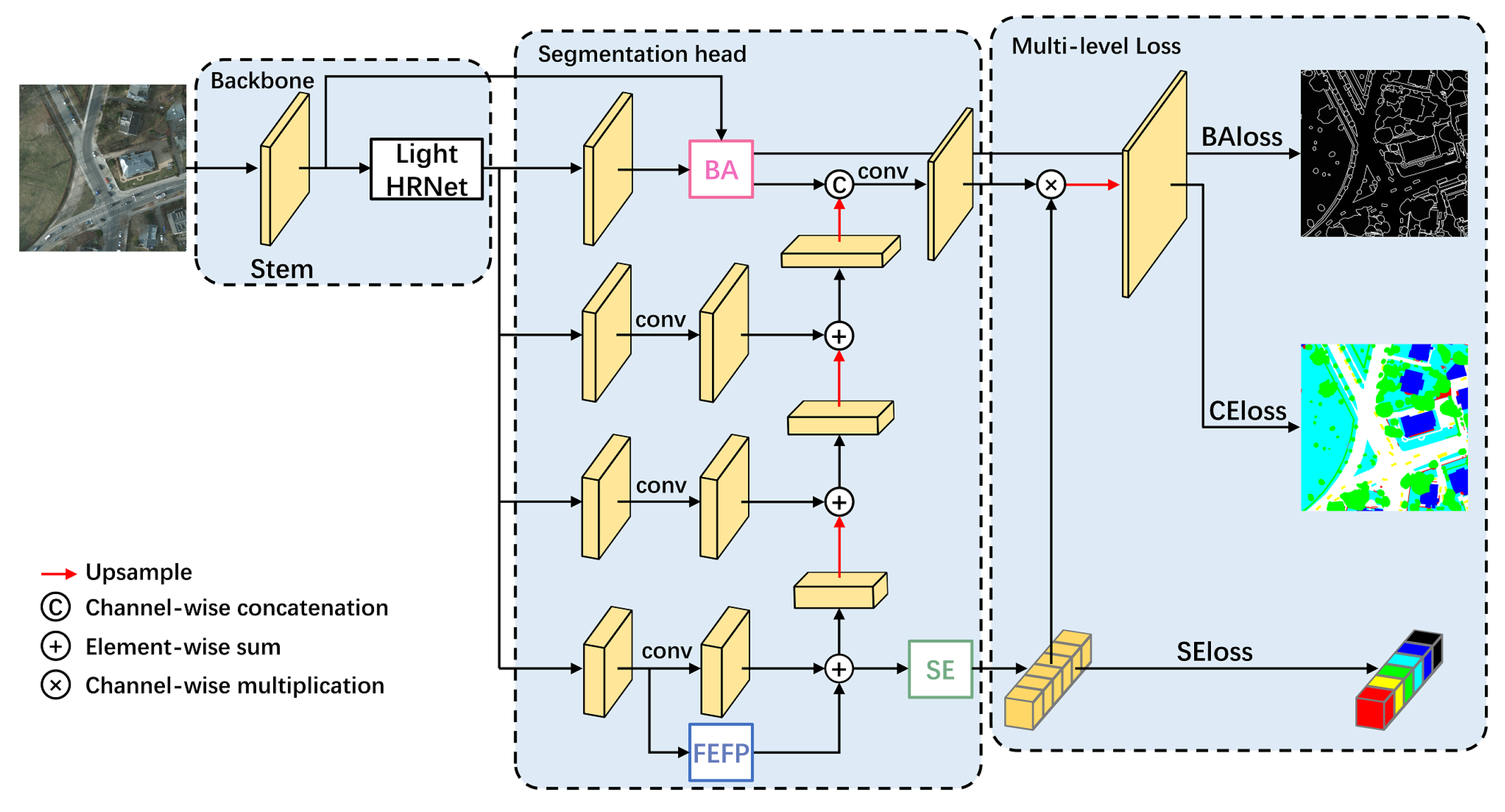
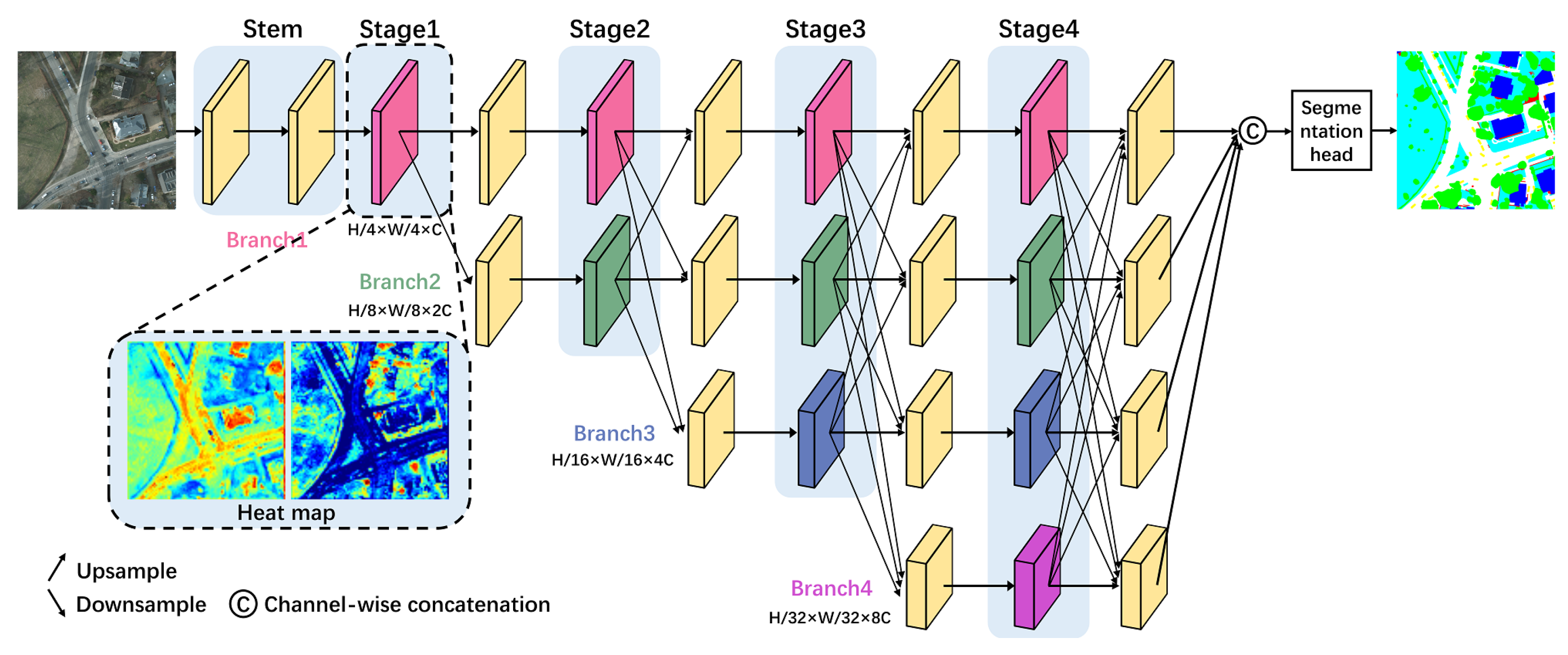
• Based on the parallel-branch architecture of HRNet, we promote the feature enhancement feature pyramid (FEFP) module to integrate the low-to-high features, improving the segmentation accuracy of each category at different scales.
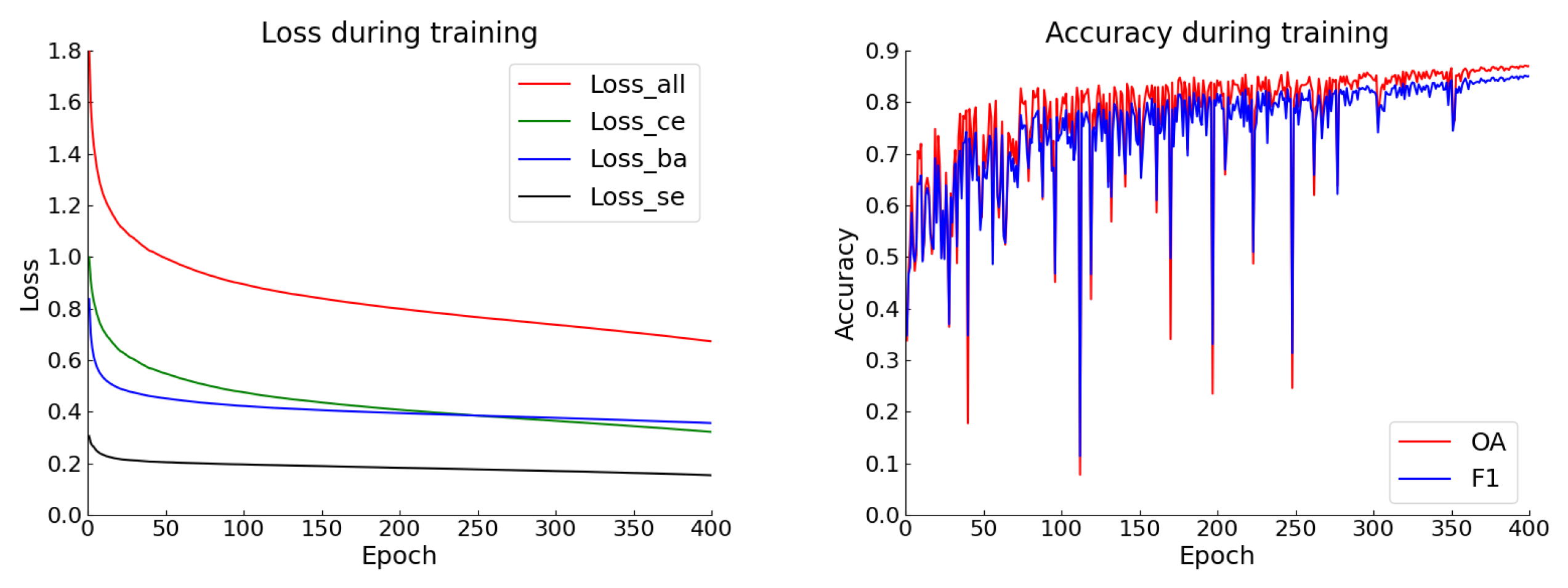
• We propose the multi-level loss functions composing of CEloss, BAloss, and SEloss to optimize the learning procedure.

2. Related Work

In this section, some related work regarding state-of-the-art remote sensing applications and the model design. The model design is composing of design of the backbone, boundary problems and attention mechanisms, where different approaches are compared coming with their advantages and shortcomings.

2.1. Remote Sensing Applications

With the development of remote sensing technology, remote sensing applications such as road detection, urban resources management and land-use mapping are applied to all fields of society. The road detection technology introduced by [23] adopted GF-3 satellite (the first C-band multi-polarized synthetic aperture rada satellite in China) to analyse the road conditions, which is helpful to improve the level of urban management. Hyperspectral remote sensing image is known with rich but redundant spectral information, Ref. [24] presented a hybrid lossless compression technique to reduce the redundant information, which could help efficiently using these RSIs. The newly developed semantic segmentation technology [25] based on deep learning adopted a more efficient technique to help for land-use mapping. Such semantic segmentation technology combined with deep learning inspired us to design a more powerful model for achieving a better performance in remote sensing segmentation.

2.2. Model Design

Combining the aforementioned three vital factors: spatial information, boundary details and global context information, three parts of the model design will be introduced respectively.

2.2.1. Design of the Backbone

Semantic segmentation is an end-to-end image segmentation method making the network directly predict the pixel-level label map. Backbone, as the feature extractor of the network, plays a paramount role in the segmentation task as the backbone performance will directly affect the “encoder” and segmentation head [26]. The LeNet in [27] is only capable of dealing with easy tasks due to the convolution layer number (only five). According to [28], the increased depth (numbers of convolution layers) can enlarge the receptive field and strengthen the discriminating ability of each pixel in comparison with increasing the width (dimensions of each convolution layer).

However, increasing the depth of the network will lead to the vanishing gradient problem, making the CNNs difficult to converge. To overcome the gradient vanishing problem, He et al. [29] proposed residual connection structure in Deep Residual Network (ResNet) model to make CNNs getting deeper even over 1000 layers without gradient vanishing problem. Based on that, some variants such as Densely Connected Convolutional Networks (DenseNet [30]) are designed to enhance the connection between residual units, and lift the ResNet a bit. In comparison with ResNet, HRNet is parallel-branch based model that can appropriately cope with multi-spectral/multi-scale image, however, such method doesn’t consider the effects of global context information and attention mechanism.

2.2.2. Boundary Problems

Boundary problems caused by the network always lead to a degraded classification performance as the network cannot treat the categories (e.g., road, vegetation and buildings) of different scales equally, so some small targets may be neglected [15]. On the contrary, it is more reliable to identify large objects because of clearer spatial information and details can be provided by the sensor. However, small objects with less spatial information are unreliable since the images taken by different sensors may be distorted and the manual labels having error.

To solve these boundary problems, the most commonly used method is skip connections, where shallow layers are fused in the CNNs due to the rich contour information [12,31]. Mou et al. [32] proposed a method that combined FCN [33] and a recurrent neural network (RNN [34]) for achieving accurate object boundary inference and semantic segmentation [35]. U-Net [10,12] adopts a number of skip connections between top layers and bottom layers at the upsampling stage to restore high-resolution information. The aforementioned two methods focus on the boundary information acquisition. Although this method is promising, there is no quantitative verification explaining that the improvement of the boundary is caused by the shallow layers. Meanwhile, the fusion method is not smooth since low-level spatial features (come from shallow layers) may damage high-level semantic features. Inspired by [9] that give an insightful discussion of the fusion algorithms, we design an explainable boundary aware module to smoothly integrate high-level and low-level features.

2.2.3. Attention Mechanisms

Attention mechanism is significant in the phase of obtaining global context information. The attention mechanisms can be divided into two parts, spatial attention mechanism and channel attention mechanism. Spatial attention mechanism is designed to capture long-range dependencies of each pixel [14]. Channel attention mechanism can obtain the relationship of different categories [36]. To lead the CNNs context-aware but also light-weight, Zhong et al. [36] proposed channel attention mechanism to obtain the relevance between different categories. Both spatial attention mechanism and channel attention mechanism yield a promising results for classification problem in [17,37], but these two methods are usually added in the segmentation head (where spatial information is damaged) and extremely heavy-weight. Therefore, the Light-weight Dual Attention module (LDA) is highly desirable at early stages.

3. Methods

In this section, we firstly present the basic HRNet, and then illustrate the framework of our proposed HRCNet, including the improvements based on HRNet. Finally, each component of HRCNet is described in details.

3.1. The Basic HRNet

As depicted in Figure 2, HRNet starts from a high-resolution subnetwork (Branch1), gradually adding high-to-low resolution subnetworks one by one to form more branches and connecting the multi-resolution subnetworks in parallel [13]. It maintains high-resolution features, providing n stages and corresponding n branches and n resolutions (here n is set as 4) [38]. After the input, two stride $3\times 3$ convolution layers (see Stem section in Figure 2) decrease the resolution to 1/4 and increase the width (number of channels of the convolution layers) to 64. The channel number C (could be selected as 32 and 48 in HRNet, which represent HRNet_W32 (W means width) and HRNet_W48, respectively) in different branches are in turn set as C, $2C$, $4C$ and $8C$, respectively. Meanwhile, the resolution decreases as H/4 × W/4, H/8 × W/8, H/16 × W/16 and H/32 × W/32. In application to semantic segmentation, the final four output features are mixed up to generate multi-scale semantic information [39]. Partial feature maps of stage1 are visualized (see Heat map), the red region represents the focus area. It can be seen that the shallow features focus more on structural information. The multi-branch parallel structure of HRNet can efficiently obtain spatial information, but it doesn’t give a consideration for global context information and boundary information.

3.2. Framework of the Proposed HRCNet

To make up for the shortcomings of HRNet, HRCNet adopts the following designs. As is shown in Figure 3, the proposed model framework consists of three sections including backbone, segmentation head, and loss functions. First, the backbone is introduced as a feature extractor to obtain semantic information aiming at downsampling (Stem) the input to expand the receptive fields and get contextual information (Light HRNet). Second, the segmentation head is applied to rebuild high-resolution features, employing the low-to-high structure to fuse the four branches after features enhancement (FEFP). Finally, the multi-level loss function is proposed to supervise the classification of the boundary, pixels, and the categories by integrating three various loss functions (BAloss, CEloss and SEloss).

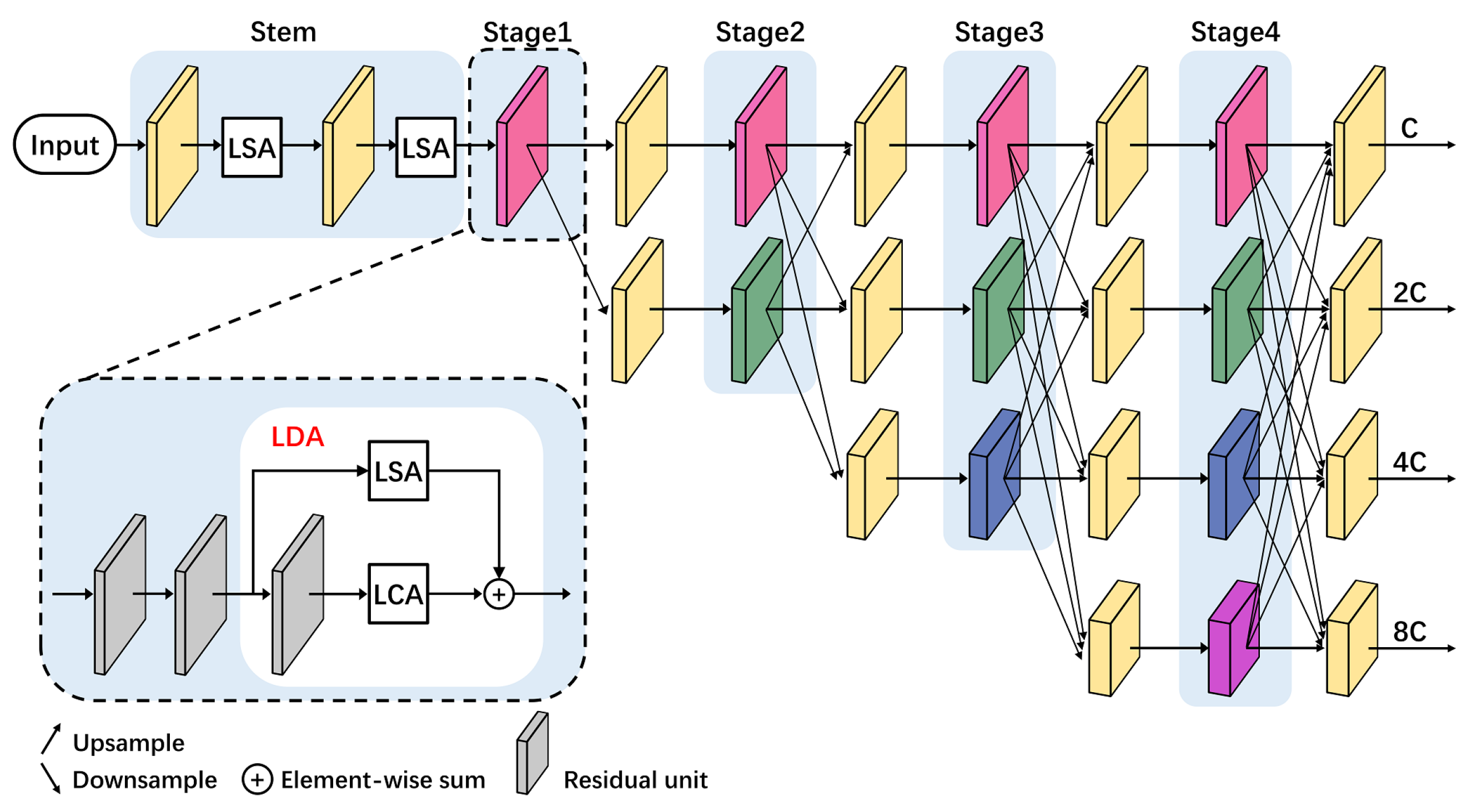
3.3. Light-Weight High-Resolution Network (Light HRNet)

In practical scenario, it is essential to guarantee the accuracy of the model and improve real-time performance. Then, the computation efficiency should be high. Inspired by light-weight semantic segmentation networks, such as BiseNet [40,41], ICNet [42], ShuffleNet [43,44], MobileNet [45,46,47], it can be found that ResNet based network (e.g., ResNet18, ResNet50, or some variant networks) is the commonly used backbone because of the high efficiency. In addition, parallel-branch architecture is proved to be efficient [48,49]. As shown in Figure 4, the light-weight HRNet architecture adopts the parallel-branch ResNet as the backbone, the number of each stage is reduced to one and the minimum residual units are kept in each branch of the same stage. Compared with these aforementioned networks, great performance improvements can be guaranteed using the proposed Light HRNet with a relatively high computation efficiency.

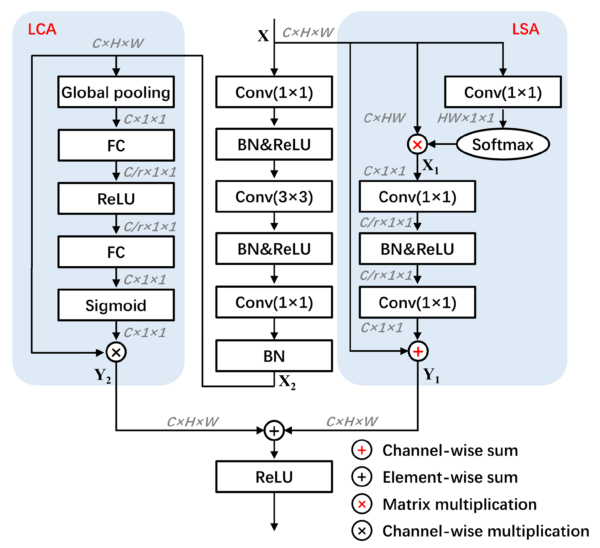
3.3.1. Light-Weight Dual Attention (LDA) Module

It can be followed from Figure 5, LDA module is composed of LSA module and LCA module to obtain spatial relevance and dimension relevance respectively, where both attention modules are light-weight. The middle branch in the LDA module is residual unit, where can be used to get feature representation. LCA module is applied behind the residual unit for that dimension relevance is high-level semantic information. LSA module is parallel with residual unit using the same input ‘X’ as residual unit, since high-resolution features are suited for obtaining spatial information. To verify the design, the position of LCA module and LSA module are exchanged, where the results indicate that the proposed LDA yields the best performance. Meanwhile, the number of LDA module is also taken into consideration to balance the computation load and final performance. The results show that one LDA module has the ability to extract the contextual information rather than using unlimited growing LDA numbers.

3.3.2. Light-Weight Spatial Attention (LSA) Module

Global Context Network (GCNet [50]) in LSA module presents that for each pixel in a H×W feature map, they almost learn the same feature map by using the conventional Non Local Networks [14] and the global context for each pixel is location independent. Therefore, to simplify the calculation, one feature map could be enough to represent the relationship between each pixel and the whole H×W pixels. Given an input feature map $\mathbf{X}\in {\mathbb{R}}^{C\times H\times W}$, the calculation details are summarized as follows:

• The first branch applies 1×1 convolution to $\mathbf{X}$ to generate a feature map with the size of ${\mathbb{R}}^{1\times H\times W}$, then reshape it to ${\mathbb{R}}^{HW\times 1\times 1}$ and softmax function is applied after that. The second branch reshapes $\mathbf{X}$ to ${\mathbb{R}}^{C\times HW}$. To this end, two branches’ results are multiplied to obtain the feature ${\mathbf{X}}_1\in {\mathbb{R}}^{C\times 1\times 1}$. $\mathit{F}(·)$ denotes convolution operation, $\alpha (·)$ denotes softmax function, $f_r(·)$ denotes reshape, and ⊗ in red denotes matrix multiplication.

  $${\mathbf{X}}_1=f_r\left(\mathbf{X}\right)\otimes \alpha \left(f_r\left(\mathit{F}\left(\mathbf{X}\right)\right)\right)$$

  (1)
• To reduce the number of parameters after the 1×1 convolution, feature ${\mathbf{X}}_1$ turns into the size of ${\mathbb{R}}^{C/r\times 1\times 1}$, where r is the bottleneck ratio usually be set to 16. Then, batch normalization (BN [51]) and activation function (ReLU [52]) are applied to improve the generalization ability of the network. After that, the feature to the size of ${\mathbb{R}}^{C\times 1\times 1}$ is restored and added to $\mathbf{X}$, getting the final output ${\mathbf{Y}}_1\in {\mathbb{R}}^{C\times H\times W}$. ⊕ in red denotes the channel-wise summation operation, and $f_{bn\&relu}(·)$ denotes BN as well as ReLU.

  $${\mathbf{Y}}_1=\mathbf{X}\oplus \mathit{F}\left(f_{bn\&relu}\left(\mathit{F}\left({\mathbf{X}}_1\right)\right)\right)$$

  (2)

3.3.3. Light-Weight Channel Attention (LCA) Module

Similar as LSA module, LCA module pays attention to the relevance between each channel (C). Given an input feature map ${\mathbf{X}}_2\in {\mathbb{R}}^{C\times H\times W}$, global average pooling is adopted to each channel of the feature map with the size of H×W to generate a global representation of the feature. Then, two fully connected layers are added with the bottleneck ratio $r=16$ to reduce the parameters. Sigmoid function works after the aforementioned operations by multiplying with ${\mathbf{X}}_2$. Here, ${\mathit{F}}_{gap}(·)$ denotes global average pooling, ${\mathit{F}}_{fc}(·)$ means fully connected layer, ⊗ denotes channel-wise multiplication, $\beta (·)$ denotes sigmoid function, and ${\mathbf{Y}}_2$ is the output of LCA module.

$${\mathbf{Y}}_2={\mathbf{X}}_2\otimes \beta \left({\mathit{F}}_{fc}\left(f_{relu}\left({\mathit{F}}_{fc}\left({\mathit{F}}_{gap}\left({\mathbf{X}}_2\right)\right)\right)\right)\right)$$

(3)

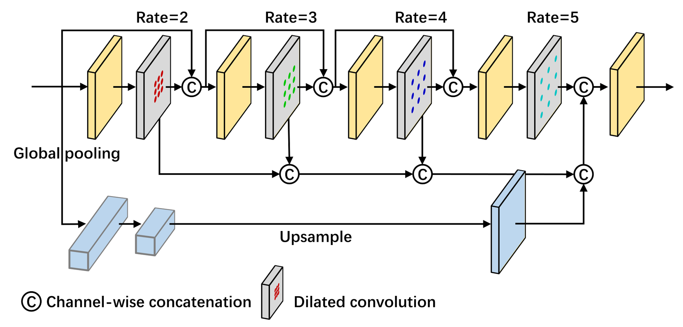
3.4. Feature Enhancement Feature Pyramid (FEFP) Module

FEFP module is proposed to replace the original fusing operation in HRNet for the aim of utilizing the multi-scale contextual information in the parallel architecture. Feature Pyramid Networks (FPN) has the ability to generate features of four scales by employing downsampling operation, and fuses the features step by step [53]. However, the multi-scale information is highly related to the original features but along with limited semantic information [54]. To overcome the defects of FPN, some improvements are made. First, four branches’ outputs of HRCNet are utilized to replace the four scales’ features without using the spatial-reduction downsampling operation. Second, the advantages of DenseNet (densely connected operation between © to strengthen information exchange among features) and Atrous Spatial Pyramid Pooling (ASPP: dilated convolution with different rates to obtain multi-scale information) module are combined together [55]. Therefore, in our work, a FEFP module is presented shown in Figure 6 by incorporating dense connections, ASPP and FPN to make the best use of high-level semantic information.

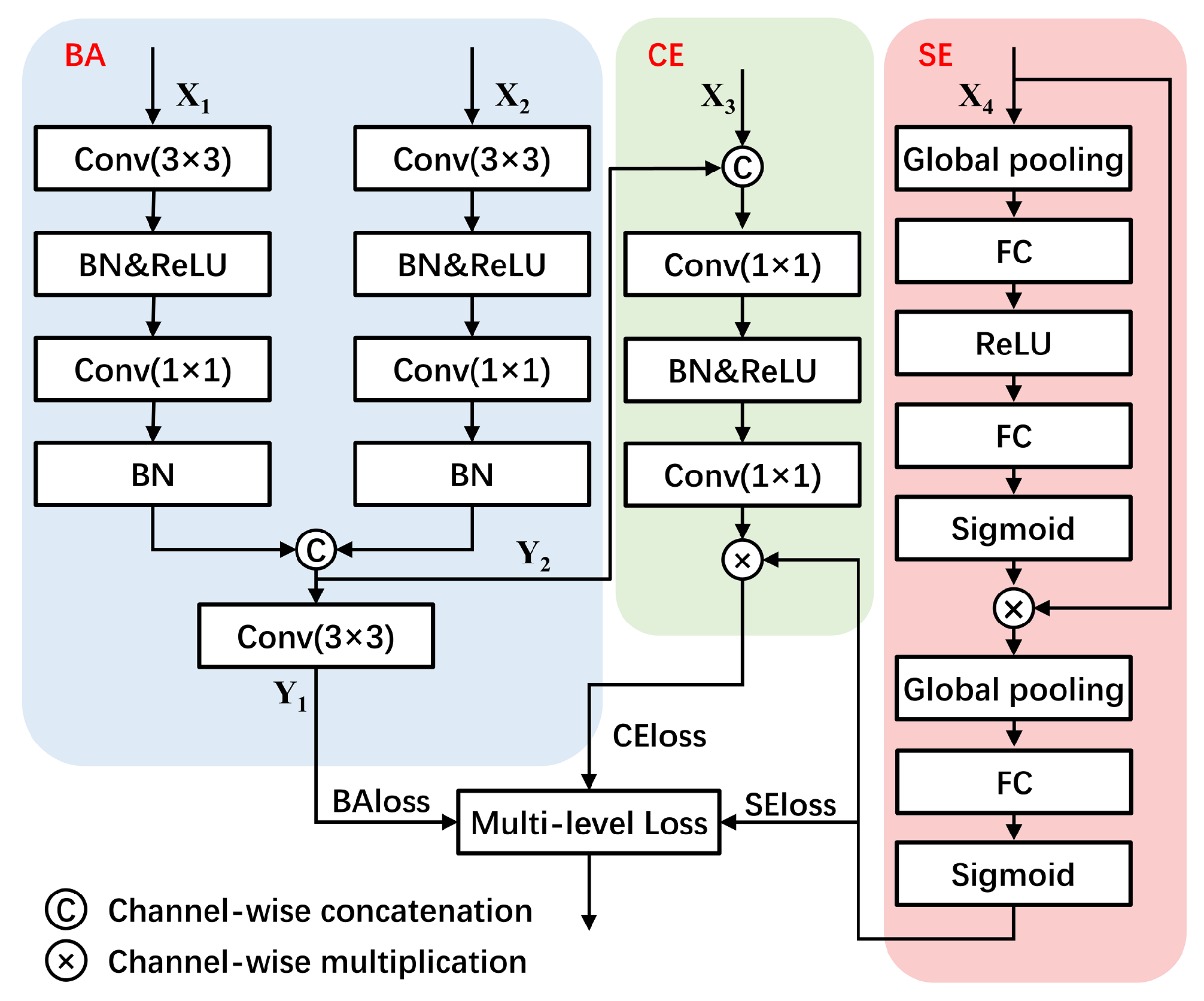
3.5. Multi-Level Loss Function

Loss function design is one of the most important step in deep learning because it guides the CNNs to optimize model parameters during the back-propagation period (e.g., loss function is normally written as the deviation value between the prediction and ground truth). As displayed in Figure 7, the conventional method applied to semantic segmentation is cross entropy loss (CEloss), which is helpful to calculate the mean of each pixel’s loss. In this proposed model, three loss functions are integrated to supervise the training data at different levels from various perspectives. Conventional CEloss is mainly employed for supervising the model in pixel-level. Boundary aware loss (BAloss) is to supervise the classification of object boundaries in region-level. The last semantic encoding loss (SEloss) is designed for supervising the classification in image-level. To help all the three loss functions work better in the proposed model, the corresponding three convolution modules are designed as follows.

3.5.1. Cross Entropy Loss for Pixel-level Classification

As is shown in CE from Figure 7, this module accepts the outputs of FEFP module (${\mathbf{X}}_3$) and BA module. The output of FEFP module represents high-level semantic information for pixel classification. The output of BA module represents high-resolution information for boundary classification. The output of CE module applies the result of SE module for auxiliary judging what categories are included in the images, since SE module could help to justify the categories from a global perspective.

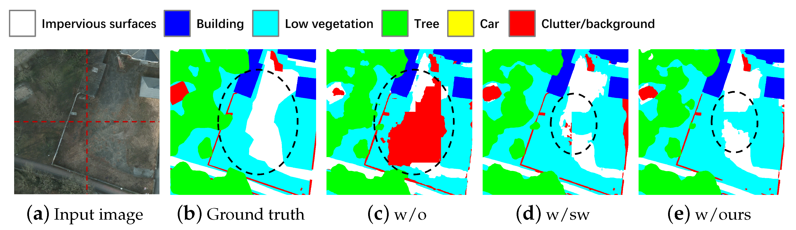
3.5.2. Boundary Aware Loss for Region-level Classification

In the segmentation task, the prediction of the boundary is often ignored because the objects boundary only accounts for a small part of the images, and the boundary is often clear once the camera is stable [56]. But for RSIs, the camera is mobile and images are photographed in an extremely long distance so that the boundary is distorted and the proportion could be much more [57]. To reduce the impact of uncertain border definitions on the evaluation, the official proposes a reference set without boundary. However, there should be another way to improve the boundary quality for the segmentation result. By referring to some conventional edge detection networks [58,59,60,61], high-resolution features are always adopted to get the boundary. However, high-resolution features are lack of semantic information, resulting in misclassification. Moreover, the boundary of the conventional boundary label is too thin resulting in the increased training difficulties.

To overcome these drawbacks, we design the boundary aware module as displayed in the left of Figure 7. It combines the outputs of the stem (${\mathbf{X}}_1$) and the first branch (${\mathbf{X}}_2$). The former possesses high resolution and structural information, the latter possesses high resolution and high-level semantic information. Both features are fused to generate binary classification results. Then, this method uses the boundary labels to supervise the results to urge the model to learn a clear boundary. The boundary labels are particularly designed as the official requirements, using a circular disc of 3 pixel radius to erode the boundary and divide the images into two regions.

3.5.3. Semantic Encoding Loss for Image-Level Classification

In the standard training process of semantic segmentation, the network is learnt from isolated pixels (per-pixel cross-entropy loss for the given input image and ground truth label), so the network may have difficulty in understanding context with no global information [22]. Some non-existing categories may be wrongly predicted for the lack of global information. Therefore, the SE module shown in the right of Figure 7 is designed to make global judgement. SEloss predicts the categories of the inputs with a very small extra computation cost. Unlike per-pixel loss, SEloss considers large and small objects equally, where is helpful to improve the segmentation accuracy of small objects. In addition, the output of the semantic encoding module is a one-dimensional vector representing the existing categories, which guides the results of semantic segmentation and filters out misclassified categories.

3.5.4. Multiple Loss Functions Fusion

The details of this proposed multi-level loss function is introduced step by step as follows:

The CEloss function as the most commonly used loss function in semantic segmentation, it is defined as:

$${\mathit{L}}_{ce}=-\sum _{i=1}^N\sum _{x=1}^H\sum _{y=1}^W\left[{\eta }_i(x,y)log\frac{e^{a_i}}{{\sum }_{i=1}^N{e}^{a_i}}+(1-{\eta }_i(x,y))log(1-\frac{e^{a_i}}{{\sum }_{i=1}^N{e}^{a_i}})\right]$$

(4)

where ${\eta }_i(x,y)\in \{0,1\}$ is the label of pixel(x, y) belonging to category i, N is the number of categories, $a_i$ is the probability of belonging to category i∈ {1, N} at pixel(x, y).

The BAloss function is commonly used in binary semantic segmentation, the loss is defined as:

$${\mathit{L}}_{ba}=-\sum _{x=1}^H\sum _{y=1}^W\left[\eta (x,y)log\frac{e^{a_0}}{e^{a_0}+e^{a_1}}+(1-\eta (x,y))log\frac{e^{a_1}}{e^{a_0}+e^{a_1}}\right]$$

(5)

where $\eta (x,y)\in \{0,1\}$ is the label of pixel(x, y), $a_0$ is the probability of boundary pixels, $a_1$ is the probability of non-boundary pixels.

The SEloss function consists of two parts, the first part turns the label to one dimensional category vector, the second part adopts multi-class binary cross entropy to calculate the loss. SEloss is defined as:

$${\mathit{L}}_{se}=-\sum _{i=1}^N\left[\eta \left(i\right)log\frac{e^{a_i}}{{\sum }_{i=1}^N{e}^{a_i}}+(1-\eta \left(i\right))log(1-\frac{e^{a_i}}{{\sum }_{i=1}^N{e}^{a_i}})\right]$$

(6)

where $\eta \left(i\right)\in \{0,1\}$ is the i th category of the category vector, $a_i$ is the probability of belonging to category i∈ {1, N}.

To obtain high-quality regional segmentation and clear boundary, we propose to define ${\mathit{L}}_{all}$ as a hybrid loss:

$${\mathit{L}}_{all}={\lambda }_1{\mathit{L}}_{ce}+{\lambda }_2{\mathit{L}}_{ba}+{\lambda }_3{\mathit{L}}_{se}$$

(7)

${\lambda }_1$, ${\lambda }_2$, and ${\lambda }_3$ are utilized to balance the losses during training, and proposed to be set as 1, 0.9, 0.2, respectively during the training process. To help under the training process, we draw the pictures (see Figure 8) (left) Epoch vs Loss, (right) Epoch vs Accuracy, OA represents overall accuracy, F1 means F1 score. Both the metrics are defined in Section 4.

4. Experiment

In this section, the datasets and experimental settings are introduced first and then two sets of experiments applied on Potsdam and Vaihingen datasets will be analysed.

4.1. Datasets

The proposed HRCNet is evaluated on the ISPRS 2D semantic benchmark datasets which include the Potsdam and Vaihingen datasets. Both datasets can be freely downloaded (http://www2.isprs.org/commissions/comm3/wg4/semantic-labeling.html). Six categories are manually labelled by six colors on these datasets, including impervious surfaces (white), building (blue), low vegetation (cyan), tree (green), car (yellow), cluster/background (red). The details of both datasets are listed as

Table 1. Datasets Settings.

Items	Potsdam		Vaihingen
	Training	Testing	Training	Testing
Sample source	ISPRS	ISPRS	ISPRS	ISPRS
Bands provided	IRRGB DSM	IRRGB DSM	IRRG DSM	IRRG DSM
Bands used	RGB	RGB	IRRG	IRRG
Ground sampling distance	5 cm	5 cm	9 cm	9 cm
Sample size (pixels)	6000 × 6000	6000 × 6000	1996 × 1995–3816 × 2550	1996 × 1995–3816 × 2550
Use size (pixels)	384 × 384	384 × 384	384 × 384	384 × 384
Sample number	24	14	16	17
Slices number	8664	13,454	817	2219
Overlapping pixels	72	192	72	192

.

4.1.1. The Potsdam Dataset

The Potsdam dataset is a high-resolution airborne image dataset collected over the city of Potsdam. It contains 38 patches (6000 × 6000 pixels), where each one consists of a true orthophoto (TOP), digital surface model (DSM), and the ground sampling distance of 5 cm. The TOP contains different bands information: near infrared (NIR), red (R), green (G), and blue (B). In this study, RGB bands are employed as features with no DSM information. Also, the dataset is divided into the training set and testing set to avoid overfitting problems (could be described as a phenomenon that highly dependent on the features of training set but performs bad on testing set), where 24 patches for training and the remaining 14 for testing. Due to the limit of hardware, we cut the sample to slices with the size of 384 × 384 pixels. And to avoid the impact of the cutting operation, 72 and 192 pixels’ overlapping are adopted in training and testing datasets, respectively. Finally, we get 8664 slices for training and 13,454 slices for testing.

4.1.2. The Vaihingen Dataset

The Vaihingen dataset shows a relatively small village with many detached buildings, where the defined object categories are the same as the Potsdam dataset. This dataset contains 33 patches with different size from 1996 × 1995 to 3816 × 2550 pixels. The ground sampling distance of the TOP (containing IR (Infrared), R, G bands) and the DSM is 9 cm. In this study, the patches of the TOP is used with 16 patches for training and 17 patches for testing. The use size and overlapping pixels are same as Potsdam datasets. Finally, 817 and 2219 slices are used for training and testing, respectively.

4.2. Experiment Settings and Evaluation Metrics

The experiments (see

Table 2. Experiment Settings.

System	Ubuntu 16.04
HPC Resource	NVIDIA RTX2080Ti GPU
DL Framework	Pytorch V1.1.0
Compiler	Pycharm 2018.3.1
Program	Python V3.5.2
Optimizer	SGD
LR Policy	Poly
Loss Functions	CEloss, BAloss, and SEloss
LR	0.01 (Potsdam), 0.08 (Vaihingen)
BS	16 (Potsdam), 8 (Vaihingen)

) are run on a high performance computing (HPC) resource NVIDIA RTX2080Ti GPU (11 GB RAM) by applying the Pytorch [62] deep learning framework. The Compiler and program are pycharm and python, respectively. The commonly used stochastic gradient descent (SGD) optimizer is adopted to direct the optimization. Learning rate (LR) and batch size (BS) are obtained through experiments. Loss functions adopt the aforementioned CEloss, BAloss and SEloss. The poly learning rate policy is used to make the training process smooth, where is expressed as follows:

$$\mathit{learning}\_\mathit{rate}=\mathit{initial}\_\mathit{learning}\_\mathit{rate}{(1-\frac{\mathit{iteration}}{\mathit{max}\_\mathit{iteration}})}^{power}$$

(8)

Initial_learning_rate is set as 0.01 and 0.08 on Potsdam and Vaihingen datasets, respectively. Iteration is calculated according to the current epoch, max_iteration is the training epoch multiplying the number of training set images. power is set as 0.9.

The evaluating metrics follow the official advice, including overall accuracy (OA) score, F1 score, precision, recall and the commonly used mean intersection over union (mIoU, the average of the six categories’ IoU) in semantic segmentation field. The formula is shown below:

$$\mathit{OA}=\frac{\mathit{TP}+\mathit{TN}}{\mathit{P}+\mathit{N}},\mathit{precision}=\frac{\mathit{TP}}{\mathit{TP}+\mathit{FP}},\mathit{recall}=\frac{\mathit{TP}}{\mathit{TP}+\mathit{FN}}$$

(9)

$${\mathit{F}}_1=2\times \frac{\mathit{precision}\times \mathit{recall}}{\mathit{precision}+\mathit{recall}},\mathit{IoU}=\frac{\mathit{TP}}{\mathit{TP}+\mathit{FP}+\mathit{FN}}$$

(10)

where P, N, TP, TN, FP, and FN represent the positive, negative, true positive, true negative, false positive, and false negative pixels in the prediction map, respectively.

4.3. Training Data and Testing Data Preparation

4.3.1. Training Data Preparation

Training data preparation is of paramount before using these data. Due to the the memory limits of the GPU hardware, it is not possible to send the whole image to the model. Here the method introduced in [1] is applied for training data generation where the original training images can be cut into small pieces remaining the objects spatial structure. These images are cut into 384 × 384 size with an overlap of 72 pixels to prevent the loss of space structure. Then, considering the importance of multi-scale information, we randomly resize the slices as different scales (0.5, 0.75, 1.0, 1.25, 1.5). When all these data augmentation methods are applied, it is equivalent to expanding the dataset by 20 times. The mentioned methods will extremely increase the diversity of the dataset, improving the applicability of the proposed model.

4.3.2. Testing Data Preparation

Testing data preparation aims at preparing the testing data before the network performance being validated. By considering the hardware limitation, the testing data also is cut into slices. Due to the demand on the completed prediction maps, we introduce three methods to restore the prediction maps, the conventional method, ‘sliding window’ method, and our proposed method. The conventional method doesn’t rebuild the edge of the slices as it employs the slices without (w/o) overlap, which lead to the spatial structure reduction. The ‘sliding window’ method (w/sw) adopts the slices with an overlap of 192 pixels, and adds the overlapping part of two slices to rebuild the edge. However, this operation may lead to a wrong prediction since the two slices cannot promise generating the same result in the overlapping part. Our proposed method (w/ours) also adopts the same slices as ‘sliding window’ method, but for the overlapping part, we only adopt the middle 192 pixels’ square, which reduces the spatial structure reduction of the edge. As is shown in

Table 3. The results evaluated by Recall (%), Precision (%), F1 (%) and overall accuracy (OA; %) based on HRNet_W32 on the Potsdam datasets.

Method	Recall	Precision	F1	OA
HRNet_W32(w/o)	89.19	88.28	88.62	88.05
HRNet_W32(w/sw)	89.57	88.62	89.08	88.45
HRNet_W32(w/ours)	89.75	88.85	89.20	88.62

, by applying our proposed method, we get nearly 0.6% promotion in each evaluating metric. Figure 9 shows the improvement in the boundary by the above three methods. The red line in the input image represents the junction of the slices. As displayed in the black circle of the prediction map, our proposed method (w/ours) gets a better performance in the junction. Consequently, the following experiments all adopt our proposed testing method.

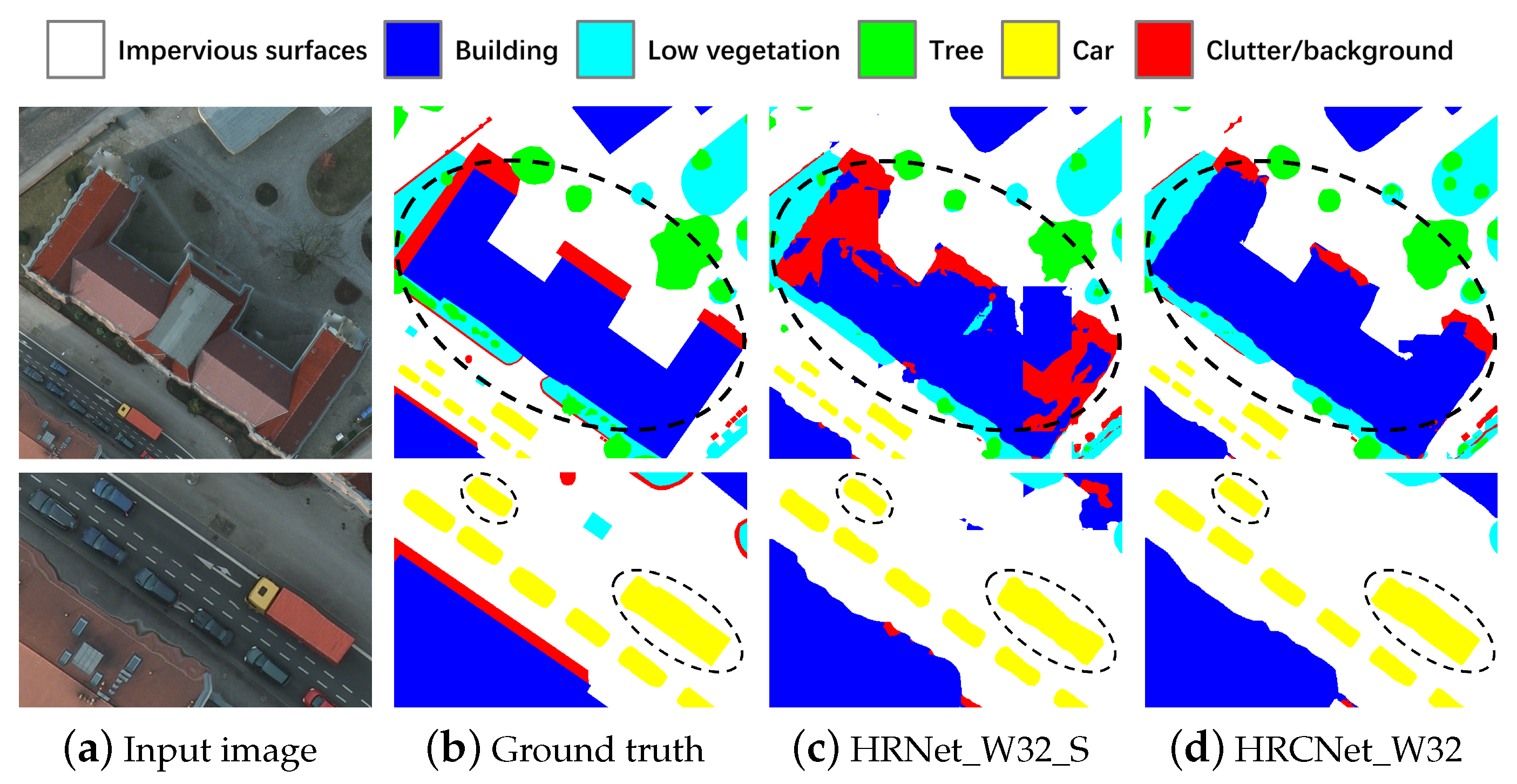
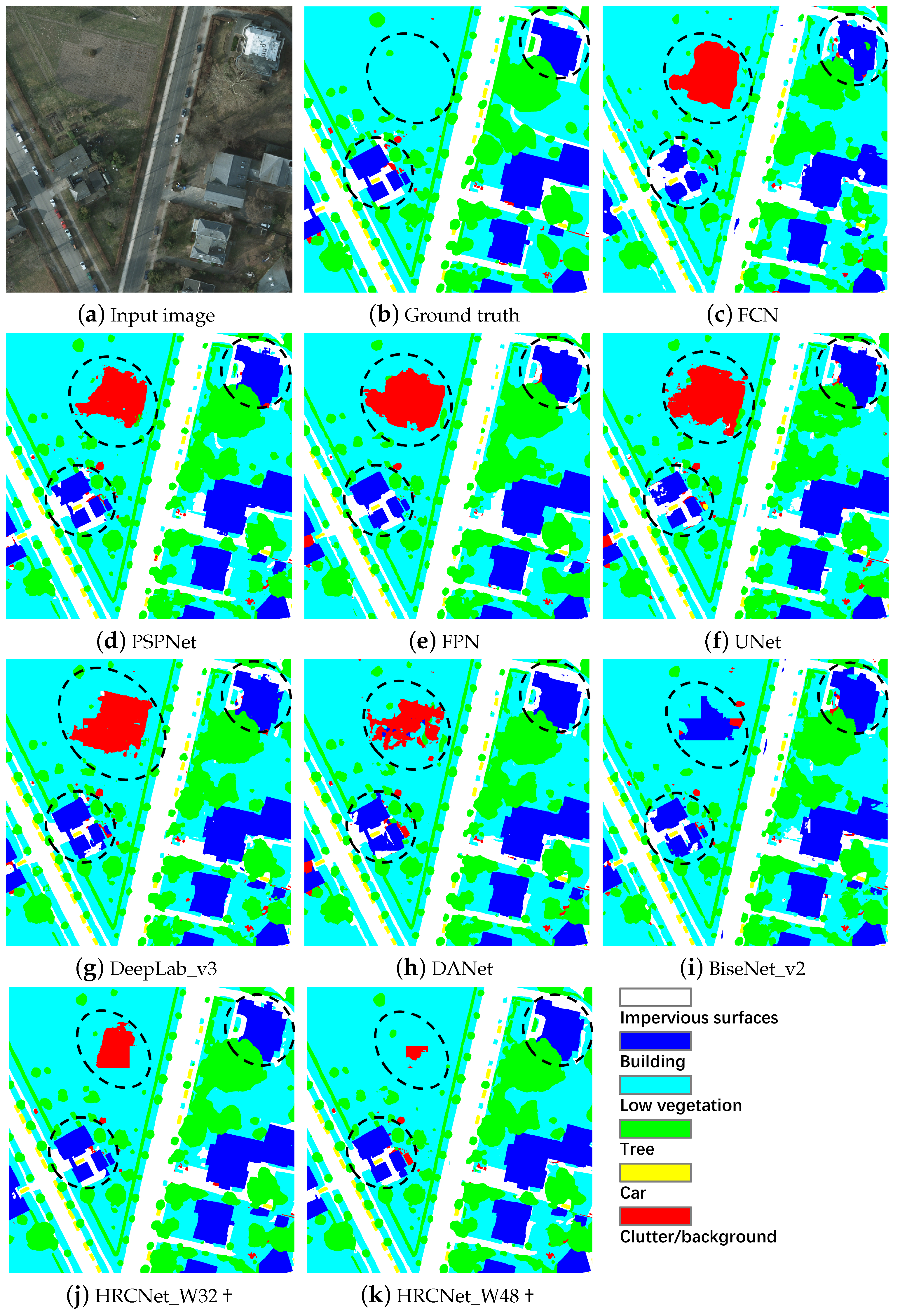
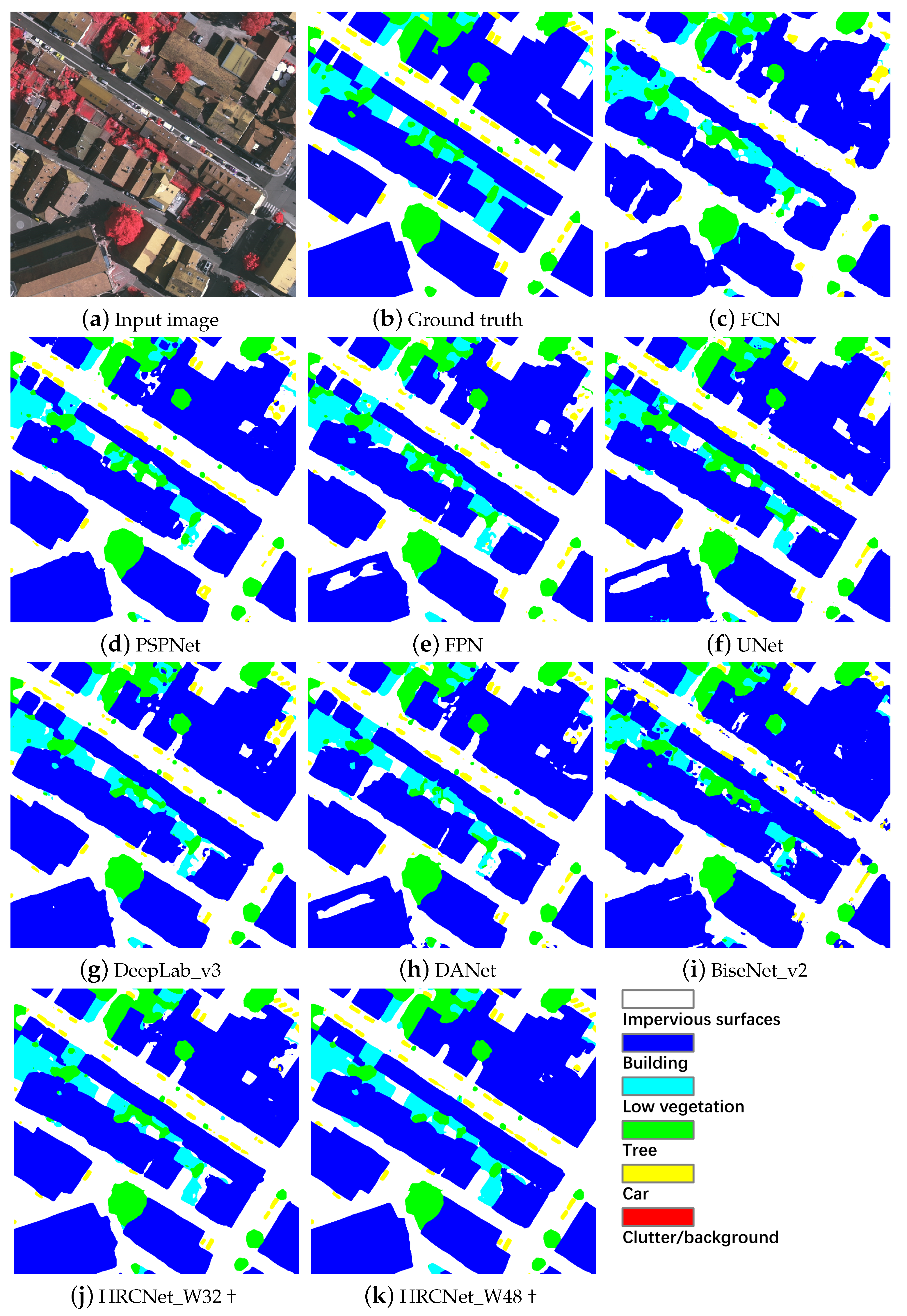
4.4. Experimental Results

According to the same network framework (Pytorch [62]) and settings, the following networks are compared with FCN [33], PSPNet [63], FPN [53], UNet [12], DeepLab_v3 [64], DANet [17] and a light-weight network BiseNet_v2 [41]. Meanwhile, the Top 1 methods called SWJ_2 [65] and HUSTW5 in Potsdam and Vaihingen 2D Semantic Labeling challenge are also compared, respectively. For ease of analysis, the best results in the table below are highlighted in bold.

Table 4. Results evaluated by Recall (%), Precision (%), F1 (%), OA (%), Giga Floating-point Operations Per Second (GFLOPS) (G) and Params (M) on the Potsdam dataset with full reference.

Method	Recall	Precision	F1	OA	GFLOPS	Params
FCN [33]	86.07	85.70	85.75	85.64	45.3	14.6
PSPNet [63]	90.13	88.95	89.45	88.78	104.0	46.5
FPN [53]	88.59	89.19	88.72	88.27	25.7	26.4
UNet [12]	89.42	88.13	88.67	87.76	70.0	12.8
DeepLab_v3 [64]	90.29	89.23	89.66	88.97	96.4	39.9
DANet [17]	90.13	88.80	89.37	88.82	115.6	47.3
BiseNet_v2 [41]	89.42	88.33	88.78	88.18	7.3	3.5
SWJ_2 [65]	89.40	89.82	89.58	89.40	/	/
HRCNet_W32	90.30	89.43	89.77	89.08	11.1	9.1
HRCNet_W32 + Flip	90.60	89.67	90.05	89.37	11.1	9.1
HRCNet_W48	90.44	89.70	89.98	89.26	52.8	59.8
HRCNet_W48 + Flip	90.69	89.90	90.20	89.50	52.8	59.8

shows the quantitative results on the Potsdam dataset where considering the boundary information (full reference set). DeepLab_v3 and PSPNet with the multi-scale fusion modules achieve a good performance in OA and F1 scores. SWJ_2 and DANet containing the attention module to obtain the global context information also perform well. BiseNet_v2 is less capable than the aforementioned four models, but with an extremely lower Giga Floating-point Operations Per Second (GFLOPS) and Params. Our proposed model HRCNet_W32 (with extremely less GFLOPS and Params) improves the Recall score by 0.9% and the F1 score by 0.19% compared with SWJ_2. In addition to HRCNet_W32, HRCNet_W48 (with Flip, Flip represents the data augmentation method called flip testing) also yields the best performance.

The results using no boundary reference set are compared in

Table 5. Results evaluated by Recall (%), Precision (%), F1 (%), OA (%), GFLOPS (G) and Params (M) on the Potsdam dataset with no boundary.

Method	Recall	Precision	F1	OA	GFLOPS	Params
SWJ_2 [65]	92.62	92.20	92.38	91.70	/	/
HRCNet_W32 + Flip	93.59	92.28	92.86	91.83	11.1	9.1
HRCNet_W48 + Flip	93.72	92.43	93.00	91.95	52.8	59.8

. The proposed two models (HRCNet_W32 and HRCNet_W48) completely surpass SWJ_2 method from all evaluation metrics.

Table 6. IoU scores (%) of each category on the Potsdam dataset.

Method	Imp Surf	Building	Low Veg	Tree	Car	Average (mIoU)
FCN [33]	81.67	88.99	71.24	72.80	79.91	78.92
PSPNet [63]	82.71	90.21	72.62	74.22	81.11	80.18
FPN [53]	81.63	89.22	71.37	73.05	79.09	78.87
UNet [12]	82.58	90.08	72.58	74.22	81.38	80.17
DeepLab_v3 [64]	82.81	89.95	72.22	74.11	82.16	80.25
DANet [17]	82.27	89.15	71.77	73.70	81.72	79.72
BiseNet_v2 [41]	81.17	87.61	71.75	73.60	81.41	79.11
HRCNet_W32 + Flip	83.16 (+0.35)	90.69 (+0.74)	72.67 (+0.45)	74.35 (+0.24)	82.73 (+0.57)	80.72 (+0.47)
HRCNet_W48 + Flip	83.58 (+0.77)	91.15 (+1.20)	73.07 (+0.85)	74.88 (+0.77)	83.32 (+1.16)	81.20 (+0.95)

displays the IoU of each category. Taking DeepLab_v3 as the baseline, the proposed HRCNet (W48) gets an average increase of 0.95%, it should be noticed that the categories building (+1.20%) and car (+1.16%) get more promotion, which proves the effectiveness of the proposed modules (LDA etc.). The prediction maps (see Figure 10) show that our proposed models achieve a better performance by focusing on the integrity of the building and the details of small objects (seen in the black circles).

Table 7. Results (%) on the Vaihingen dataset with full reference.

Method	Recall	Precision	F1	OA
FCN [33]	80.89	83.14	81.46	87.11
PSPNet [63]	84.10	84.86	84.15	87.17
FPN [53]	82.21	84.50	82.94	86.70
UNet [12]	85.01	84.46	84.44	87.14
DeepLab_v3 [64]	84.38	85.09	84.42	87.32
DANet [17]	83.89	84.65	83.95	87.07
BiseNet_v2 [41]	83.16	84.77	83.57	86.88
HUSTW5	83.32	86.20	84.50	88.60
HRCNet_W32	85.48	85.75	85.31	87.90
HRCNet_W32 + Flip	85.71	86.12	85.60	88.11
HRCNet_W32 + Flip + MS	85.30	86.40	85.48	88.29
HRCNet_W48	86.27	85.57	85.65	88.07
HRCNet_W48 + Flip	86.53	85.96	85.97	88.33
HRCNet_W48 + Flip + MS	86.29	86.47	86.07	88.56

displays the results on the Vaihingen dataset. GFLOPS and Params are not taken into account since HUSTW5 is not available. Based on the full reference set, the HRCNet_W48 (with Flip and MS, where MS represents the data augmentation method called Multi-Scale testing ) improves the Recall by 2.97%, the Precision by 0.27%, and the F1 by 1.57% compared with HUSTW5, respectively. The supplementary results using various methods on the no boundary reference set are shown in

Table 8. Results (%) on the Vaihingen dataset with no boundary, “†” means data augmentation (Flip and Multi-scale (MS) testing) methods.

Method	Recall	Precision	F1	OA
HUSTW5 [65]	87.36	89.36	88.24	91.60
HRCNet_W32 †	90.71	89.70	89.86	92.03
HRCNet_W48 †	91.49	89.80	90.30	92.30

, and it can be noticed that the proposed method achieves the best performance over HUSTW5 (“†” represents Flip and MS [66]).

Table 9. Intersection over union (IoU) scores (%) of each category on the Vaihingen dataset, “†” means data augmentation (Flip and MS testing) methods.

Method	Imp Surf	Building	Low Veg	Tree	Car	Average (mIoU)
FCN [33]	77.68	82.33	63.94	74.35	51.83	70.02
PSPNet [63]	78.90	84.26	65.34	75.14	56.18	71.96
FPN [53]	77.65	82.72	64.34	74.43	52.11	70.25
UNet [12]	79.02	84.46	65.23	75.13	57.07	72.18
DeepLab_v3 [64]	79.23	83.70	64.88	75.14	57.54	72.10
DANet [17]	78.55	82.10	64.18	74.80	56.36	71.20
BiseNet_v2 [41]	77.70	78.78	63.23	74.98	53.24	69.58
HRCNet_W32 †	80.21 (+1.19)	85.87 (+1.41)	66.01 (+0.78)	75.88 (+0.75)	58.40 (+1.33)	73.27 (+1.09)
HRCNet_W48 †	81.05 (+2.03)	86.65 (+2.19)	66.91 (+1.68)	76.63 (+1.50)	59.31 (+2.24)	74.11 (+1.93)

shows the IoU scores on Vaihingen dataset. On the baseline of UNet, our model gets the same conclusion as the experiments on Potadam dataset for achieving a greater improvement of large object (building) and small object (car).

The improvements using Vaihingen dataset is much more than using Potsdam dataset. The likely reason is due to the sensing image composition, where the category of building accounting for a large proportion in the whole image in Vaihingen dataset. Therefore, it is particularly essential for the model to obtain the spatial information and boundary details. Figure 11 displays the ability of each model to extract spatial information. It could be seen in the boundary of the buildings, our proposed models could predict a sharp boundary and complete structure in Vaihingen dataset.

5. Discussion

In this section, first, two sets of ablation experiments are used to verify the effectiveness of proposed modules (LDA, FEFP and multi-level loss function). Then, the reason for improving the accuracy is analysed and the improvements of the segmentation results are visualized. Finally, the improvements compared to previous research and the limitations of the proposed methods are discussed.

5.1. Ablation Experiments

To demonstrate the effectiveness of our proposed modules, two ablation experiments are performed on the Potsdam dataset. In addition, to eliminate the possibility of the improvement caused by the increase of parameters and computation load, a comparative study is conducted before and after adding different architectures. The basic parameters are abbreviated as Params, the unit is MByte (M) and the calculation amount is expressed by GFLOPS (Giga Floating-point Operations Per Second). The following experiments are performed with the same setting.

As is shown in

Table 10. The ablation experiments evaluated by F1 (%) and OA (%) about the proposed architectures.

Method	LSA	LCA	FEFP	F1	OA
HRNet_W32_S				89.20	88.62
HRNet_W32_S	✓			89.34	88.75
HRNet_W32_S		✓		89.32	88.71
HRNet_W32_S	✓	✓		89.42	88.81
HRNet_W32_S(HRCNet_W32)	✓	✓	✓	89.60	88.93
HRNet_W48				89.46	88.83
HRNet_W48	✓			89.53	88.94
HRNet_W48		✓		89.51	88.92
HRNet_W48	✓	✓		89.57	88.99
HRNet_W48(HRCNet_W48)	✓	✓	✓	89.74	89.13

, LSA module, LCA module, and FEFP module are performed by HRNet_W32_S (S means a light-weight HRNet_W32) and HRNet_W48, respectively. Based on the HRNet_W32_S model, LSA and LCA modules yield an approximate increase of 0.1% in F1 and OA scores, and two modules promote 0.19% in OA score and 0.22% in F1 score by integrating these two modules. The proposed HRCNet_W32 integrating LSA, LCA and FEFP modules achieves 0.40% and 0.31% promotion in F1 and OA scores. On the basis of HRNet_W48 model, LSA and LCA modules working together promote 0.16% in OA score and 0.11% in F1 score, where both scores are less than the improvement of the HRNet_W32_S model. The overall improvements of this proposed architecture using W32 and W48 are 0.40%/0.28% in OA score and 0.31%/0.30% in F1 score. The possible reason is caused by that the same modules are more difficult to perform well on a stronger model (HRNet_W48). However, it still can be concluded that the proposed method (HRCNet) is advantageous in both W32 and W48 compared with the single module based network.

It can be visually see from

Table 11. The ablation experiments evaluated by F1 (%) and OA (%) about the multi-level loss functions.

Method	CEloss	BAloss	SEloss	F1	OA
HRCNet_W32	✓			89.60	88.93
HRCNet_W32	✓	✓		89.72	89.05
HRCNet_W32	✓		✓	89.70	89.01
HRCNet_W32	✓	✓	✓	89.77	89.08
HRCNet_W48	✓			89.74	89.13
HRCNet_W48	✓	✓		89.90	89.25
HRCNet_W48	✓		✓	89.84	89.15
HRCNet_W48	✓	✓	✓	89.98	89.26

where utilized various three multi-level loss functions (CEloss, BAloss, and SEloss) in the ablation experiment. In comparison with CEloss based and BAloss based loss functions, the performance of OA and F1 scores accommodating CEloss, BAloss and SEloss methods outperforms other two methods on two models (W32: 89.08, 89.77; W48: 89.26, 89.98). From the results, we get a conclusion that compared with SEloss, the BAloss brings greater improvement as the proposed model could easily recognize which categories are included in the image (the significance of SEloss), but distinguishing the boundary still be challenging if without BAloss.

Table 12. The ablation experiments evaluated by F1 (%), OA (%), GFLOPS (G) and Params (M) about the multi-level loss functions.

Method	Recall	Precision	F1	OA	GFLOPS	Params
HRNet_W32_S	89.75	88.85	89.20	88.62	13.0	9.8
HRCNet_W32	90.30	89.43	89.77	89.08	11.1	9.1
HRNet_W48	89.97	89.14	89.46	88.83	52.8	62.8
HRCNet_W48	90.44	89.70	89.98	89.26	52.8	59.8

shows the proposed model with the decreasing of Params and GLOPS, the OA and F1 scores achieved the better performance.

To directly verify the model performance combining both high-resolution information and low-resolution information of the image, the segmentation results of HRNet_W32_S and HRCNet_W32 are visualised in Figure 12. Some categories such as building and tree represent global perception, car represents the attention in details.

5.2. Improvements and Limitations

Our proposed model focuses on obtaining global context information (LDA module), spatial information (HRNet structure), boundary information (BA module) at the same time. The literature on remote sensing segmentation, such as UNet (spatial information) and DeepLab_V3 (global context information) only focuses one aspect and are not good enough. As for the boundary information, very few works highlight it. Moreover, we first propose to combine the three loss functions (CEloss, BAloss and SEloss) with our proposed modules to improve the aforementioned three vital factors. The visualized prediction maps shown in Figure 9, Figure 10, Figure 11 and Figure 12 display the improvements of the boundary details and overall segmentation performance in case of adopting our methods. Especially, Table 6 and Table 9 show the increase of IoU scores on Potsdam and Vaihingen datasets. The IoU scores of category building and car are above the average IoU (mIoU) scores, which means our models extremely improve the segmentation performance of large and small objects due to the proposed modules.

Also, there are some limitations of our models and the experimental results. The most important part is the choice of band information. In this paper, we choice the RGB bands and IRRG bands on Potsdam and Vaihingen datasets respectively, both of the bands are composing of three divided bands. [7] expressed the combination of different bands will get different results so that proposed several evaluation methods for the combination modes. Moreover, it is obvious that more bands more information. Therefore, the combination modes and the number of bands should be specially considered. Additional explanation, we have tried to apply RGB bands with additional DSM band but get very few promotions. We attribute this to the diversity of the DSM band, which should be especially designed to fit the present models.

6. Conclusions

In this paper, the CNNs based semantic segmentation of remote sensing images is conducted. Because of the significance of spatial information, global context information and boundary details, a novel architecture named High-Resolution Context Extraction Network (HRCNet) is proposed. In comparison with HRNet in weakly obtaining the global context information and boundary information, the proposed method designs different modules to overcome such problems. LDA module is designed to adopt light-weight dual attention mechanisms to make the model focus on the relevance of different categories. Moreover, FEFP module is employed with high accuracy (W48 achieves 89.13% OA and 89.74% F1 scores on the full reference set) and less computation load (W32 consumes only 11.1 G GFLOPS and 9.1 M Params) to make the use of multi-scale contextual information in comparison with HRNet. Finally, boundary aware (BA) are employed to greatly improve the objects boundary (see Figure 12) and multi-level loss function is applied to optimize the model. The proposed architecture shows an improvement over existing state-of-the-art networks and yields the best performance, which achieves 92.0% and 92.3% overall accuracy scores on Potsdam and Vaihingen datasets, respectively. With the increasing physical information of remote sensing images, in the future the DSM information can be considered to further improve the network performance.

References

1. Zhang, J.; Lin, S.; Ding, L.; Bruzzone, L. Multi-Scale Context Aggregation for Semantic Segmentation of Remote Sensing Images. Remote Sens. 2020, 12, 701. [Google Scholar] [CrossRef] [Green Version]
2. Gkioxari, G.; Girshick, R.; Malik, J. Actions and attributes from wholes and parts. In Proceedings of the IEEE International Conference on Computer Vision, Santiago, Chile, 7–13 December 2015; pp. 2470–2478. [Google Scholar]
3. Ren, S.; He, K.; Girshick, R.; Sun, J. Faster r-cnn: Towards real-time object detection with region proposal networks. IEEE Trans. Pattern Anal. Mach. Intell. 2016, 39, 1137–1149. [Google Scholar] [CrossRef] [PubMed] [Green Version]
4. Lin, T.Y.; Goyal, P.; Girshick, R.; He, K.; Dollár, P. Focal loss for dense object detection. In Proceedings of the IEEE international conference on computer vision, Venice, Italy, 22–29 October 2017; pp. 2980–2988. [Google Scholar]
5. Dai, J.; Li, Y.; He, K.; Sun, J. R-fcn: Object detection via region-based fully convolutional networks. arXiv 2016, arXiv:1605.06409. [Google Scholar]
6. Zhang, W.; Liljedahl, A.K.; Kanevskiy, M.; Epstein, H.E.; Jones, B.M.; Jorgenson, M.T.; Kent, K. Transferability of the Deep Learning Mask R-CNN Model for Automated Mapping of Ice-Wedge Polygons in High-Resolution Satellite and UAV Images. Remote Sens. 2020, 12, 1085. [Google Scholar] [CrossRef] [Green Version]
7. Bhuiyan, M.A.E.; Witharana, C.; Liljedahl, A.K. Use of Very High Spatial Resolution Commercial Satellite Imagery and Deep Learning to Automatically Map Ice-Wedge Polygons across Tundra Vegetation Types. J. Imaging 2020, 6, 137. [Google Scholar] [CrossRef]
8. Bhuiyan, M.A.E.; Witharana, C.; Liljedahl, A.K.; Jones, B.M.; Daanen, R.; Epstein, H.E.; Kent, K.; Griffin, C.G.; Agnew, A. Understanding the Effects of Optimal Combination of Spectral Bands on Deep Learning Model Predictions: A Case Study Based on Permafrost Tundra Landform Mapping Using High Resolution Multispectral Satellite Imagery. J. Imaging 2020, 6, 97. [Google Scholar] [CrossRef]
9. Witharana, C.; Bhuiyan, M.A.E.; Liljedahl, A.K.; Kanevskiy, M.; Epstein, H.E.; Jones, B.M.; Daanen, R.; Griffin, C.G.; Kent, K.; Jones, M.K.W. Understanding the synergies of deep learning and data fusion of multispectral and panchromatic high resolution commercial satellite imagery for automated ice-wedge polygon detection. ISPRS J. Photogramm. Remote Sens. 2020, 170, 174–191. [Google Scholar] [CrossRef]
10. Wang, Y.; Liang, B.; Ding, M.; Li, J. Dense Semantic Labeling with Atrous Spatial Pyramid Pooling and Decoder for High-Resolution Remote Sensing Imagery. Remote Sens. 2019, 11, 20. [Google Scholar] [CrossRef] [Green Version]
11. Badrinarayanan, V.; Kendall, A.; Cipolla, R. SegNet: A Deep Convolutional Encoder-Decoder Architecture for Image Segmentation. IEEE Trans. Pattern Anal. Mach. Intell. 2017, 39, 2481–2495. [Google Scholar] [CrossRef]
12. Ronneberger, O.; Fischer, P.; Brox, T. U-net: Convolutional Networks for Biomedical Image Segmentation. In Proceedings of the International Conference on Medical Image Computing And Computer-Assisted Intervention, Munich, Germany, 5–9 October 2015; pp. 234–241. [Google Scholar]
13. Sun, K.; Xiao, B.; Liu, D.; Wang, J. Deep high-resolution representation learning for human pose estimation. In Proceedings of the IEEE Conference on Computer Vision and Pattern Recognition, Long Beach, CA, USA, 16–20 June 2019; pp. 5693–5703. [Google Scholar]
14. Wang, X.; Girshick, R.; Gupta, A.; He, K. Non-local neural networks. In Proceedings of the IEEE Conference on Computer Vision and Pattern Recognition, Salt Lake City, UT, USA, 18–22 June 2018; pp. 7794–7803. [Google Scholar]
15. Takikawa, T.; Acuna, D.; Jampani, V.; Fidler, S. Gated-scnn: Gated shape cnns for semantic segmentation. In Proceedings of the IEEE International Conference on Computer Vision, Seoul, Korea, 27 October–2 November 2019; pp. 5229–5238. [Google Scholar]
16. Huang, Z.; Wang, X.; Huang, L.; Huang, C.; Wei, Y.; Liu, W. Ccnet: Criss-cross attention for semantic segmentation. In Proceedings of the IEEE International Conference on Computer Vision, Seoul, Korea, 27 October–2 November 2019; pp. 603–612. [Google Scholar]
17. Fu, J.; Liu, J.; Tian, H.; Li, Y.; Bao, Y.; Fang, Z.; Lu, H. Dual attention network for scene segmentation. In Proceedings of the IEEE Conference on Computer Vision and Pattern Recognition, Long Beach, CA, USA, 16–20 June 2019; pp. 3146–3154. [Google Scholar]
18. Li, X.; Li, X.; Zhang, L.; Cheng, G.; Shi, J.; Lin, Z.; Tan, S.; Tong, Y. Improving semantic segmentation via decoupled body and edge supervision. arXiv 2020, arXiv:2007.10035. [Google Scholar]
19. Zhen, M.; Wang, J.; Zhou, L.; Li, S.; Shen, T.; Shang, J.; Fang, T.; Quan, L. Joint Semantic Segmentation and Boundary Detection using Iterative Pyramid Contexts. In Proceedings of the IEEE/CVF Conference on Computer Vision and Pattern Recognition, Seattle, WA, USA, 14–19 June 2020; pp. 13666–13675. [Google Scholar]
20. De Boer, P.T.; Kroese, D.P.; Mannor, S.; Rubinstein, R.Y. A tutorial on the cross-entropy method. Ann. Oper. Res. 2005, 134, 19–67. [Google Scholar] [CrossRef]
21. Qin, X.; Zhang, Z.; Huang, C.; Gao, C.; Dehghan, M.; Jagersand, M. Basnet: Boundary-aware salient object detection. In Proceedings of the IEEE Conference on Computer Vision and Pattern Recognition, Long Beach, CA, USA, 16–20 June 2019; pp. 7479–7489. [Google Scholar]
22. Zhang, H.; Dana, K.; Shi, J.; Zhang, Z.; Wang, X.; Tyagi, A.; Agrawal, A. Context encoding for semantic segmentation. In Proceedings of the IEEE conference on Computer Vision and Pattern Recognition, Salt Lake City, UT, USA, 18–22 June 2018; pp. 7151–7160. [Google Scholar]
23. Sun, Z.; Lin, D.; Wei, W.; Woźniak, M.; Damaševičius, R. Road Detection Based on Shearlet for GF-3 Synthetic Aperture Radar Images. IEEE Access 2020, 8, 28133–28141. [Google Scholar] [CrossRef]
24. Afjal, M.I.; Uddin, P.; Mamun, A.; Marjan, A. An efficient lossless compression technique for remote sensing images using segmentation based band reordering heuristics. Int. J. Remote Sens. 2020, 42, 756–781. [Google Scholar] [CrossRef]
25. Chen, G.; Li, C.; Wei, W.; Jing, W.; Woźniak, M.; Blažauskas, T.; Damaševičius, R. Fully convolutional neural network with augmented atrous spatial pyramid pool and fully connected fusion path for high resolution remote sensing image segmentation. Appl. Sci. 2019, 9, 1816. [Google Scholar] [CrossRef] [Green Version]
26. Tian, Z.; He, T.; Shen, C.; Yan, Y. Decoders matter for semantic segmentation: Data-dependent decoding enables flexible feature aggregation. In Proceedings of the IEEE Conference on Computer Vision and Pattern Recognition, Long Beach, CA, USA, 16–20 June 2019; pp. 3126–3135. [Google Scholar]
27. Lecun, Y.; Bottou, L.; Bengio, Y.; Haffner, P. Gradient-based learning applied to document recognition. Proc. IEEE 1998, 86, 2278–2324. [Google Scholar] [CrossRef] [Green Version]
28. Simonyan, K.; Zisserman, A. Very deep convolutional networks for large-scale image recognition. arXiv 2014, arXiv:1409.1556. [Google Scholar]
29. He, K.; Zhang, X.; Ren, S.; Sun, J. Deep residual learning for image recognition. In Proceedings of the IEEE Conference on Computer Vision and Pattern Recognition, Las Vegas, NV, USA, 27–30 June 2016; pp. 770–778. [Google Scholar]
30. Huang, G.; Liu, Z.; Van Der Maaten, L.; Weinberger, K.Q. Densely connected convolutional networks. In Proceedings of the IEEE Conference on Computer Vision and Pattern Recognition, Honolulu, HI, USA, 21–26 July 2017; pp. 4700–4708. [Google Scholar]
31. He, S.; Du, H.; Zhou, G.; Li, X.; Mao, F.; Zhu, D.; Xu, Y.; Zhang, M.; Huang, Z.; Liu, H.; et al. Intelligent Mapping of Urban Forests from High-Resolution Remotely Sensed Imagery Using Object-Based U-Net-DenseNet-Coupled Network. Remote Sens. 2020, 12, 3928. [Google Scholar] [CrossRef]
32. Mou, L.; Zhu, X.X. RiFCN: Recurrent network in fully convolutional network for semantic segmentation of high resolution remote sensing images. arXiv 2018, arXiv:1805.02091. [Google Scholar]
33. Long, J.; Shelhamer, E.; Darrell, T. Fully convolutional networks for semantic segmentation. In Proceedings of the IEEE Conference on Computer Vision and Pattern Recognition, Boston, MA, USA, 7–12 June 2015; pp. 3431–3440. [Google Scholar]
34. Zaremba, W.; Sutskever, I.; Vinyals, O. Recurrent neural network regularization. arXiv 2014, arXiv:1409.2329. [Google Scholar]
35. Yang, G.; Zhang, Q.; Zhang, G. EANet: Edge-Aware Network for the Extraction of Buildings from Aerial Images. Remote Sens. 2020, 12, 2161. [Google Scholar] [CrossRef]
36. Hu, J.; Shen, L.; Sun, G. Squeeze-and-excitation networks. In Proceedings of the IEEE Conference on Computer Vision and Pattern Recognition, Salt Lake City, UT, USA, 18–22 June 2018; pp. 7132–7141. [Google Scholar]
37. Yuan, Y.; Chen, X.; Wang, J. Object-contextual representations for semantic segmentation. arXiv 2019, arXiv:1909.11065. [Google Scholar]
38. Wang, J.; Sun, K.; Cheng, T.; Jiang, B.; Deng, C.; Zhao, Y.; Liu, D.; Mu, Y.; Tan, M.; Wang, X.; et al. Deep high-resolution representation learning for visual recognition. IEEE Trans. Pattern Anal. Mach. Intell. 2020, 99, 1. [Google Scholar] [CrossRef] [PubMed] [Green Version]
39. Sun, K.; Zhao, Y.; Jiang, B.; Cheng, T.; Xiao, B.; Liu, D.; Mu, Y.; Wang, X.; Liu, W.; Wang, J. High-resolution representations for labeling pixels and regions. arXiv 2019, arXiv:1904.04514. [Google Scholar]
40. Yu, C.; Wang, J.; Peng, C.; Gao, C.; Yu, G.; Sang, N. Bisenet: Bilateral segmentation network for real-time semantic segmentation. In Proceedings of the European Conference on Computer Cision (ECCV), Munich, Germany, 8–14 September 2018; pp. 325–341. [Google Scholar]
41. Yu, C.; Gao, C.; Wang, J.; Yu, G.; Shen, C.; Sang, N. BiSeNet V2: Bilateral Network with Guided Aggregation for Real-time Semantic Segmentation. arXiv 2020, arXiv:2004.02147. [Google Scholar]
42. Zhao, H.; Qi, X.; Shen, X.; Shi, J.; Jia, J. Icnet for real-time semantic segmentation on high-resolution images. In Proceedings of the European Conference on Computer Vision (ECCV), Munich, Germany, 8–14 September 2018; pp. 405–420. [Google Scholar]
43. Zhang, X.; Zhou, X.; Lin, M.; Sun, J. Shufflenet: An extremely efficient convolutional neural network for mobile devices. In Proceedings of the IEEE Conference on Computer Vision and Pattern Recognition, Salt Lake City, UT, USA, 18–22 June 2018; pp. 6848–6856. [Google Scholar]
44. Ma, N.; Zhang, X.; Zheng, H.T.; Sun, J. Shufflenet v2: Practical guidelines for efficient cnn architecture design. In Proceedings of the European Conference on Computer Vision (ECCV), Munich, Germany, 8–14 September 2018; pp. 116–131. [Google Scholar]
45. Howard, A.G.; Zhu, M.; Chen, B.; Kalenichenko, D.; Wang, W.; Weyand, T.; Andreetto, M.; Adam, H. Mobilenets: Efficient convolutional neural networks for mobile vision applications. arXiv 2017, arXiv:1704.04861. [Google Scholar]
46. Sandler, M.; Howard, A.; Zhu, M.; Zhmoginov, A.; Chen, L.C. Mobilenetv2: Inverted residuals and linear bottlenecks. In Proceedings of the IEEE Conference on Computer Vision and Pattern Recognition, Salt Lake City, UT, USA, 18–22 June 2018; pp. 4510–4520. [Google Scholar]
47. Howard, A.; Sandler, M.; Chu, G.; Chen, L.C.; Chen, B.; Tan, M.; Wang, W.; Zhu, Y.; Pang, R.; Vasudevan, V.; et al. Searching for mobilenetv3. In Proceedings of the IEEE International Conference on Computer Vision, Seoul, Korea, 27 October–2 November 2019; pp. 1314–1324.
48. Tan, M.; Le, Q.V. Efficientnet: Rethinking model scaling for convolutional neural networks. arXiv 2019, arXiv:1905.11946. [Google Scholar]
49. Radosavovic, I.; Kosaraju, R.P.; Girshick, R.; He, K.; Dollár, P. Designing network design spaces. In Proceedings of the IEEE/CVF Conference on Computer Vision and Pattern Recognition, Seattle, WA, USA, 14–19 June 2020; pp. 10428–10436. [Google Scholar]
50. Cao, Y.; Xu, J.; Lin, S.; Wei, F.; Hu, H. Gcnet: Non-local networks meet squeeze-excitation networks and beyond. In Proceedings of the IEEE International Conference on Computer Vision Workshops, Seoul, Korea, 27 October–2 November 2019. [Google Scholar]
51. Ioffe, S.; Szegedy, C. Batch normalization: Accelerating deep network training by reducing internal covariate shift. arXiv 2015, arXiv:1502.03167. [Google Scholar]
52. Glorot, X.; Bordes, A.; Bengio, Y. Deep sparse rectifier neural networks. In Proceedings of the Fourteenth International Conference on Artificial Intelligence and Statistics, Fort Lauderdale, FL, USA, 11–13 April 2011; pp. 315–323. [Google Scholar]
53. Lin, T.Y.; Dollár, P.; Girshick, R.; He, K.; Hariharan, B.; Belongie, S. Feature pyramid networks for object detection. In Proceedings of the IEEE Conference on Computer Vision and Pattern Recognition, Honolulu, HI, USA, 21–26 July 2017; pp. 2117–2125. [Google Scholar]
54. Guo, S.; Jin, Q.; Wang, H.; Wang, X.; Wang, Y.; Xiang, S. Learnable Gated Convolutional Neural Network for Semantic Segmentation in Remote-Sensing Images. Remote Sens. 2019, 11, 1922. [Google Scholar] [CrossRef] [Green Version]
55. Yang, M.; Yu, K.; Zhang, C.; Li, Z.; Yang, K. Denseaspp for semantic segmentation in street scenes. In Proceedings of the IEEE Conference on Computer Vision and Pattern Recognition, Salt Lake City, UT, USA, 18–22 June 2018; pp. 3684–3692. [Google Scholar]
56. Wang, H.; Wang, Y.; Zhang, Q.; Xiang, S.; Pan, C. Gated Convolutional Neural Network for Semantic Segmentation in High-Resolution Images. Remote Sens. 2017, 9, 446. [Google Scholar] [CrossRef] [Green Version]
57. Ahmadi, S.; Zoej, M.V.; Ebadi, H.; Moghaddam, H.A.; Mohammadzadeh, A. Automatic urban building boundary extraction from high resolution aerial images using an innovative model of active contours. Int. J. Appl. Earth Obs. Geoinf. 2010, 12, 150–157. [Google Scholar] [CrossRef]
58. Luo, L.; Xue, D.; Feng, X. EHANet: An Effective Hierarchical Aggregation Network for Face Parsing. Appl. Sci. 2020, 10, 3135. [Google Scholar] [CrossRef]
59. He, J.; Zhang, S.; Yang, M.; Shan, Y.; Huang, T. Bi-directional cascade network for perceptual edge detection. In Proceedings of the IEEE Conference on Computer Vision and Pattern Recognition, Long Beach, CA, USA, 16–20 June 2019; pp. 3828–3837. [Google Scholar]
60. Zeng, C.; Zheng, J.; Li, J. Real-Time Conveyor Belt Deviation Detection Algorithm Based on Multi-Scale Feature Fusion Network. Algorithms 2019, 12, 205. [Google Scholar] [CrossRef] [Green Version]
61. Liu, Y.; Cheng, M.M.; Hu, X.; Wang, K.; Bai, X. Richer convolutional features for edge detection. In Proceedings of the IEEE Conference on Computer Vision and Pattern Recognition, Honolulu, HI, USA, 21–26 July 2017; pp. 3000–3009. [Google Scholar]
62. Paszke, A.; Gross, S.; Chintala, S.; Chanan, G.; Yang, E.; DeVito, Z.; Lin, Z.; Desmaison, A.; Antiga, L.; Lerer, A. Automatic differentiation in pytorch. In Proceedings of the Conference on Neural Information Processing Systems, Long Beach, CA, USA, 4–9 December 2017. [Google Scholar]
63. Zhao, H.; Shi, J.; Qi, X.; Wang, X.; Jia, J. Pyramid scene parsing network. In Proceedings of the IEEE Conference on Computer Vision and Pattern Recognition, Honolulu, HI, USA, 21–26 July 2017; pp. 2881–2890. [Google Scholar]
64. Chen, L.C.; Papandreou, G.; Schroff, F.; Adam, H. Rethinking atrous convolution for semantic image segmentation. arXiv 2017, arXiv:1706.05587. [Google Scholar]
65. Wang, J.; Shen, L.; Qiao, W.; Dai, Y.; Li, Z. Deep feature fusion with integration of residual connection and attention model for classification of VHR remote sensing images. Remote Sens. 2019, 11, 1617. [Google Scholar] [CrossRef] [Green Version]
66. Tian, Z.; Shen, C.; Chen, H.; He, T. Fcos: Fully convolutional one-stage object detection. In Proceedings of the IEEE International Conference on Computer Vision, Seoul, Korea, 27 October–2 November 2019; pp. 9627–9636. [Google Scholar]
Figure 1. The overall framework of our model.
Remotesensing 13 00071 g001
Figure 2. Illustrating the architecture of HRNet. The rectangular blocks represent the feature maps, and ’⟶’ represents the convolution operation. Stem is the downsampling process.
Remotesensing 13 00071 g002
Figure 3. The overall architecture is divided into three parts, from left to right are the backbone, segmentation head, and loss functions.
Remotesensing 13 00071 g003
Figure 4. Light-weight dual attention (LDA) module is applied to the four stages (Stage1, Stage2, Stage3, and Stage4).
Remotesensing 13 00071 g004
Figure 5. Detailed design of LDA module.
Remotesensing 13 00071 g005
Figure 6. Framework of feature enhancement feature pyramid (FEFP) module.
Remotesensing 13 00071 g006
Figure 7. Framework of designed multiple loss functions.
Remotesensing 13 00071 g007
Figure 8. Loss and accuracy during the training process.
Remotesensing 13 00071 g008
Figure 9. Comparation of the three postprocessing methods on the Potsdam dataset.
Remotesensing 13 00071 g009
Figure 10. Prediction maps of the compared methods on the Potsdam dataset. “†” means using data augmentation (Flip testing) methods.
Remotesensing 13 00071 g010
Figure 11. The prediction maps of the above methods on the Vaihingen dataset. “†” means using data augmentation (Flip and MS testing) methods.
Remotesensing 13 00071 g011
Figure 12. Our proposed modules significantly improve the segmentation of large objects, and for small objects, the boundary segmentation is smoother.
Remotesensing 13 00071 g012