Article

The Grain for Green Program Intensifies Trade-Offs between Ecosystem Services in Midwestern Shanxi, China

1
School of Ecology and Nature Conservation, Beijing Forestry University, Beijing 100083, China
2
Hohhot Meteorological Bureau, Hohhot 010020, China
3
State Key Laboratory of Urban and Regional Ecology, Research Center for Eco-Environmental Sciences, Chinese Academy of Sciences, Beijing 100085, China
*
Author to whom correspondence should be addressed.
Remote Sens. 2021, 13(19), 3966; https://doi.org/10.3390/rs13193966
Submission received: 30 August 2021 / Revised: 26 September 2021 / Accepted: 30 September 2021 / Published: 3 October 2021
(This article belongs to the Topic Climate Change and Environmental Sustainability)

Abstract

:
Ecological engineering is a widely used strategy to address environmental degradation and enhance human well-being. A quantitative assessment of the impacts of ecological engineering on ecosystem services (ESs) is a prerequisite for designing inclusive and sustainable engineering programs. In order to strengthen national ecological security, the Chinese government has implemented the world’s largest ecological project since 1999, the Grain for Green Program (GFGP). We used a professional model to evaluate the key ESs in Lvliang City. Scenario analysis was used to quantify the contribution of the GFGP to changes in ESs and the impacts of trade-offs/synergy. We used spatial regression to identify the main drivers of ES trade-offs. We found that: (1) From 2000 to 2018, the contribution rates of the GFGP to changes in carbon storage (CS), habitat quality (HQ), water yield (WY), and soil conservation (SC) were 140.92%, 155.59%, −454.48%, and 92.96%, respectively. GFGP compensated for the negative impacts of external environmental pressure on CS and HQ, and significantly improved CS, HQ, and SC, but at the expense of WY. (2) The GFGP promotes the synergistic development of CS, HQ, and SC, and also intensifies the trade-off relationships between WY and CS, WY and HQ, and WY and SC. (3) Land use change and urbanization are significantly positively correlated with the WY–CS, WY–HQ, and WY–SC trade-offs, while increases in NDVI helped alleviate these trade-offs. (4) Geographically weighted regression explained 90.8%, 94.2%, and 88.2% of the WY–CS, WY–HQ, and WY–SC trade-offs, respectively. We suggest that the ESs’ benefits from the GFGP can be maximized by controlling the intensity of land use change, optimizing the development of urbanization, and improving the effectiveness of afforestation. This general method of quantifying the impact of ecological engineering on ESs can act as a reference for future ecological restoration plans and decision-making in China and across the world.

1. Introduction

Ecosystem services (ESs) refer to all the benefits that human beings obtain directly or indirectly from the natural ecosystem to meet and maintain their living needs [1,2]. The Millennium Ecosystem Assessment (MEA) divides ESs into four basic types, including regulating services (e.g., soil conservation and carbon storage), provisioning services (e.g., water and timber), supporting services (e.g., biodiversity conservation and nutrient cycling), and cultural services (e.g., forest recreation) [2,3]. Human development patterns over the last few centuries have detrimentally affected the health and resilience of natural ecosystems [3,4]. Declines in ESs have been observed at global and regional scales, and these declines pose a significant threat to human well-being [2,5]. Ecological engineering is a widely adopted countermeasure that attempts to mitigate the contradiction between human development and ecosystem protection [6,7]. Ecological engineering aims to increase the sustainable supply of ESs by repairing or improving ecosystem functioning [8,9]. At present, global investment in the development of ecological engineering amounts to billions of dollars per year [9], and quantitative assessment of the effects of ecological engineering on ESs has attracted the attention of many managers, research organizations, and researchers [10].
ESs are good indicators for evaluating the ecological benefits of ecological engineering, as they effectively connect human well-being and the natural environment [1,11]. ES trade-offs occur when the increase of a certain ES is at the cost of reducing another ES [2,12]. Therefore, revealing the influencing factors of ES trade-offs is crucial to maintaining the sustainable supply of multiple ESs [12,13]. The frequent conversion between land use types caused by high-intensity human activities is the main cause of ES declines [14,15]. Rebuilding the ecological functioning of degraded ecosystems by changing land use patterns and intensity of use is the main aim of most ecological projects [8,16], which will have strong impacts on the supply and trade-offs between ESs [17,18]. Ecological engineering that unilaterally promotes a single ES makes it difficult to maximize ecological benefits [19], and may even negatively affect ecosystem functioning and cause other services to decline [20,21].
Ecological degradation is one of the main reasons for the increasing frequency of natural disasters [22]. In order to achieve carbon neutrality and strengthen national ecological security, the Chinese government has implemented the world’s largest ecological project since 1999: the Grain for Green Program (GFGP) [23]. With the implementation of the GFGP, vegetation cover has increased significantly [24] and various ESs, such as biodiversity and climate regulation, have been significantly improved [25]. However, large-scale planting of non-native vegetation not only leads to a significant increase in water consumption and evapotranspiration [26], which aggravates the potential conflict between regional ecosystem functioning and human demand for water resources [27], but also further challenges the achievement of balance between green and grain land, especially in arid regions [28,29]. This has rendered uncertain the sustainability of the ecological benefits of the GFGP. Therefore, quantitative assessment of the impacts of ecological engineering on ESs and analysis of the dominant factors driving ES trade-offs are prerequisites for the design of inclusive and sustainable ecological engineering [30].
In the context of rapid socio-economic development, most studies have confirmed that the GFGP can improve ESs and change the relationship between ecosystem support services and regulation services [31,32]. However, this change is influenced by multiple factors, such as natural, anthropogenic, climatic, and socio-economic factors [33]. There are few studies that quantify the contribution rate of ecological engineering to changes in ESs and the impacts of ecological engineering on the relationship between different ESs. In this study, we focus on Lvliang City, Shanxi Province, an area typical of the GFGP. This region has serious soil erosion and is a typical ecologically fragile zone. Our specific objectives are: (1) to quantify the contribution rate of the GFGP to changes in ESs; (2) to analyze the impacts of the GFGP on the trade-offs and synergy between ESs; and (3) to identify the factors influencing the trade-offs between ESs and put forward suggestions for promoting the inclusive and sustainable development of the GFGP. This research should serve as a reference for future ecological engineering projects in China and around the world.

2. Materials and Methods
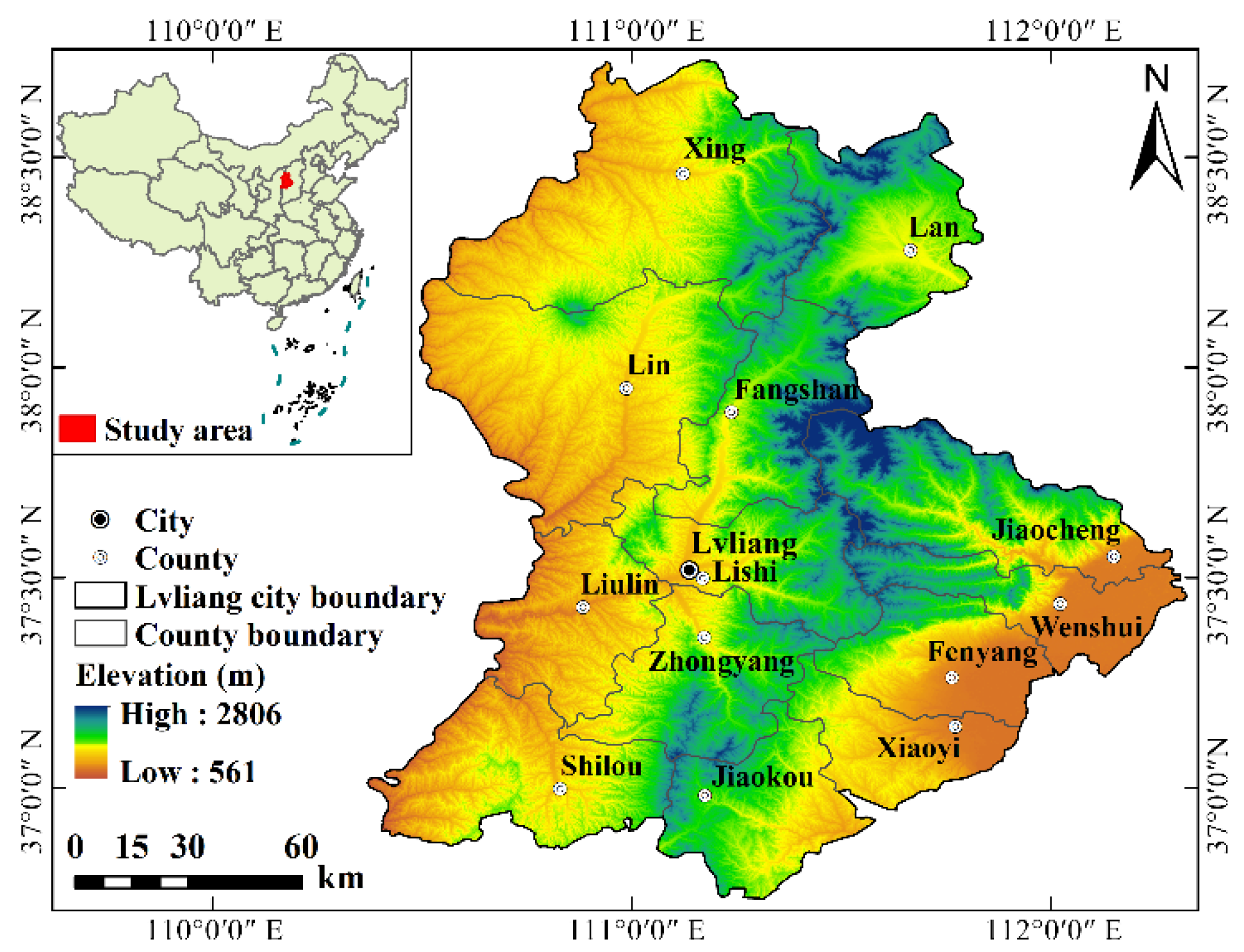
2.1. Study Area

Lvliang City is located in the east-central region of China’s Loess Plateau and the western region of Shanxi Province, and has an area of about 21,100 km2 (Figure 1). Lvliang City has a continental monsoon climate with four distinct seasons, synchronized rain and heat, and sufficient sunlight. The average annual temperature is between 0.4 °C and 12.2 °C, and the average annual precipitation is between 438 and 588 mm. The elevation of the study area ranges from 561 to 2806 m a.s.l., with high terrain in the middle of the study area and lower terrain on the edges (Figure 1). Vegetation cover in the mountains of the central and eastern regions is relatively high, and human activities and industrial development are mainly concentrated in the southeastern plains; the western loess hilly regions have broken terrain, barren soil, and sparse vegetation [34,35]. Due to the low coverage rate of surface vegetation coupled with the landform type of prevalent ravines, the area has serious soil erosion and is typically an ecologically fragile area [34]. In recent years, because of the GFGP, the vegetation coverage rate in this area has increased significantly, the functions of various ecosystems such as climate regulation and soil conservation have improved significantly, and ESs have, accordingly, changed significantly [24,35].

2.2. Data Sources and Descriptions

In this study, we used multi-source data products, such as land use, meteorology, soil, and digital elevation models, to evaluate ESs. Detailed descriptions and data sources are shown in Table 1. In ArcGIS 10.2, all data are converted to the same projected coordinate system (WGS_1984_UTM_Zone_49N), and the “Resample” tool is used to unify the raster data resolution to 30 m.

2.3. Quantifying Ecosystem Services

The InVEST model is used to quantify four key ESs: water yield (WY), soil conservation (SC), habitat quality (HQ), and carbon storage (CS). WY is calculated based on the difference between annual average precipitation and actual annual evapotranspiration [29,36]. SC refers to the erosion control ability of the ecosystem to prevent soil loss and the ability to store and maintain sediment [36,37]. The sediment delivery ratio module calculates soil conservation services based on the difference between potential (under extremely degraded conditions without vegetation cover) and actual (under current land cover and management conditions) soil loss [19,36,37]. HQ refers to the ability to provide resources and environmental conditions for the survival and development of species or populations, which depends on the abundance of natural resources [36,38]. The habitat quality module calculates the HQ according to the habitat suitability of each land use type, the impact distance and weight of threat factors, and the sensitivity of each land use type to threat factors [36,38]. Through previous studies [38,39,40,41], we determined the impact distance and weight of threat factors, the habitat suitability of each land use type, and the sensitivity parameters to each threat factor (Tables S1 and S2). The carbon module quantifies CS using previous local research on the carbon density of different land use types [42,43,44] (Table S3). To avoid the influence of abnormal climate fluctuations in a single year, we selected the average rainfall and temperature from 2000 to 2018 as the general results from the study area [45,46]. Table 2 provide greater detail on the process of assessment of each ES.

2.4. Calculation of Trade-Offs Between Ecosystem Services

Correlation analysis is an effective tool to identify relationships between pairs of ESs, with significant negative correlations representing trade-offs and positive correlations representing synergies [47]. The size of the Pearson correlation coefficient indicates the strength of the trade-off and synergy relationships [47]. Obviously, this method ignores the difference in the geographical space of the change rate of the ES trade-offs. The root mean squared error (RMSE) quantifies the average difference between the standard deviation of a single ES and the average ES’s standard deviation [47,48]. The dispersion degree of the standard deviation of distance of average ESs is described, and reflects the difference in the geographical space of the change rate of the ES’s trade-offs [49,50]. Therefore, this study uses the RMSE to quantify the trade-offs between ESs. To eliminate the influence of ES unit differences, we first standardize the value of each ES.
ES i = ES i , o b s ES i , m i n ES i , m a x ES i , m i n .
where ESi is the standardized value; ESi,obs is the raw value; and ESi,min and ESi,max are the minimum and maximum values of the i ESs, respectively. RMSE is calculated as follows:
R M S E = 1 n 1 i = 1 n ( ES i ES ¯ ) 2
where E S ¯ is the expected value of n kinds of ESs. In two dimensions, RMSE represents the distance from the coordinate point to the diagonal, and the relative position of the coordinate point represents the relative benefit of a certain ecosystem service [49]. Lu et al. [48] and Luo et al. [50] provide detailed instructions and procedures for the calculation of such trade-offs.

2.5. Actual Land Use Changes and Scenarios

The local administrative department of the GFGP provided vector data for the implementation area of the GFGP in Lvliang City as of the end of 2018. We set up a scenario where the GFGP was not implemented and quantified the impact of the GFGP on regional ESs by comparing this alternative scenario with the actual scenario.
(1) Actual scenario: we evaluated ESs before (2000) and after (2018) the implementation of the GFGP based on actual land use. By comparing ESs in 2000 and 2018, we can understand actual changes of ESs under the implementation of the GFGP.
(2) Alternative scenarios where the GFGP was not implemented (2018S): this is a simulated scenario. We assume that during the period 2000–2018, the actual GFGP implementation area did not implement the GFGP; that is, the land use types remained, unchanged, at their state in 2000, while the land use types in other regions were consistent with actual changes. By comparing ESs in 2018S and 2018, we were able to quantify the impact of the GFGP on ESs.
Terrain fragmentation due to soil erosion is the main cause of ecological degradation in the Loess Plateau [51]. The design and implementation of the GFGP on the sub-watershed scale to carry out comprehensive control of soil erosion has achieved good results [19,52]. In addition, as a physical geographical unit, the sub-watershed scale can more accurately reflect biophysical characteristics [19]. Therefore, we obtained the average value of each ES at the sub-watershed scale through the Zonal Statistics tool in ArcGIS 10.2. At the sub-watershed scale, the impact of GFGP on ESs was quantified and the trade-offs among ESs and their influencing factors were analyzed.

2.6. Geographically Weighted Regression Model

Previous studies have confirmed that there are obvious geographical differences in ESs [53,54]. It is difficult for the classic global regression to reflect the differences in the relationship between ES trade-offs and influencing factors in geographic space, and not fully reflect actual local processes [55]. Geographically weighted regression (GWR) obtains local coefficients by minimizing residuals, taking into account differences in the spatial variation in the relationship between ES trade-offs and influencing factors, which improves the reliability of the model [56].
ESs and their trade-off relationships are affected by factors such as land use [57], climate [58], vegetation [19], geomorphology [59], and urbanization [60]. We selected eight influencing factors to include in our model: the dynamic degree of comprehensive land use change (LUD; Refer to Li et al. [61] method for calculation), annual average temperature (TEM), NDVI, annual average precipitation (PRE), percentage of construction land (CON), elevation (DEM), slope (SLO), and potential evapotranspiration (PET) (Table S4 provides detailed calculation methods or sources). To avoid the influence of multicollinearity, all factors were tested for multicollinearity in SPSS 21, and the factors with VIF greater than five were eliminated (Table S5). These preliminary analyses left us with LUD, NDVI, PRE, DEM, and CON as independent variables and the trade-off relationships between ESs as dependent variables for our GWR model. The lower the AICc value of the model output, the more concise the model and the more reliable the regression estimation. The higher adjusted R2 indicates a higher explanatory power and a better fit [56]. The mathematical expression of the model is as follows:
y i = β 0 ( u i ,   v i ) + j = 1 p β j ( u i , v i ) x i j + ε i ,   i { 1 , 2 , , n }
where y is the dependent variable; (ui, vi) is the spatial location of the i-th sample; β0 (ui, vi) is the intercept; p is the number of influencing factors; xij represents the independent variables; βj (ui, vi) is the estimated coefficient of the i-th sample for the j-th driving factors; and ɛi is the error term.

3. Results

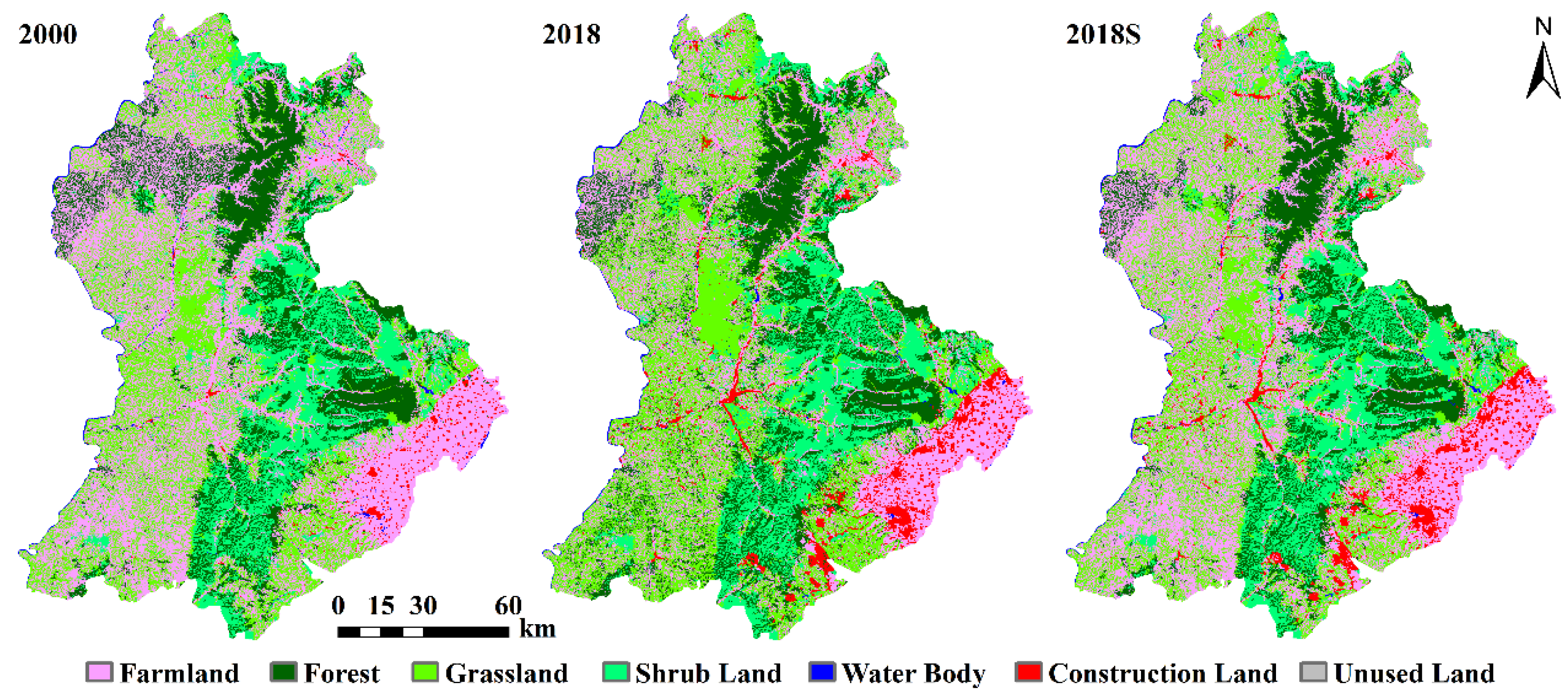
3.1. Land Use Change
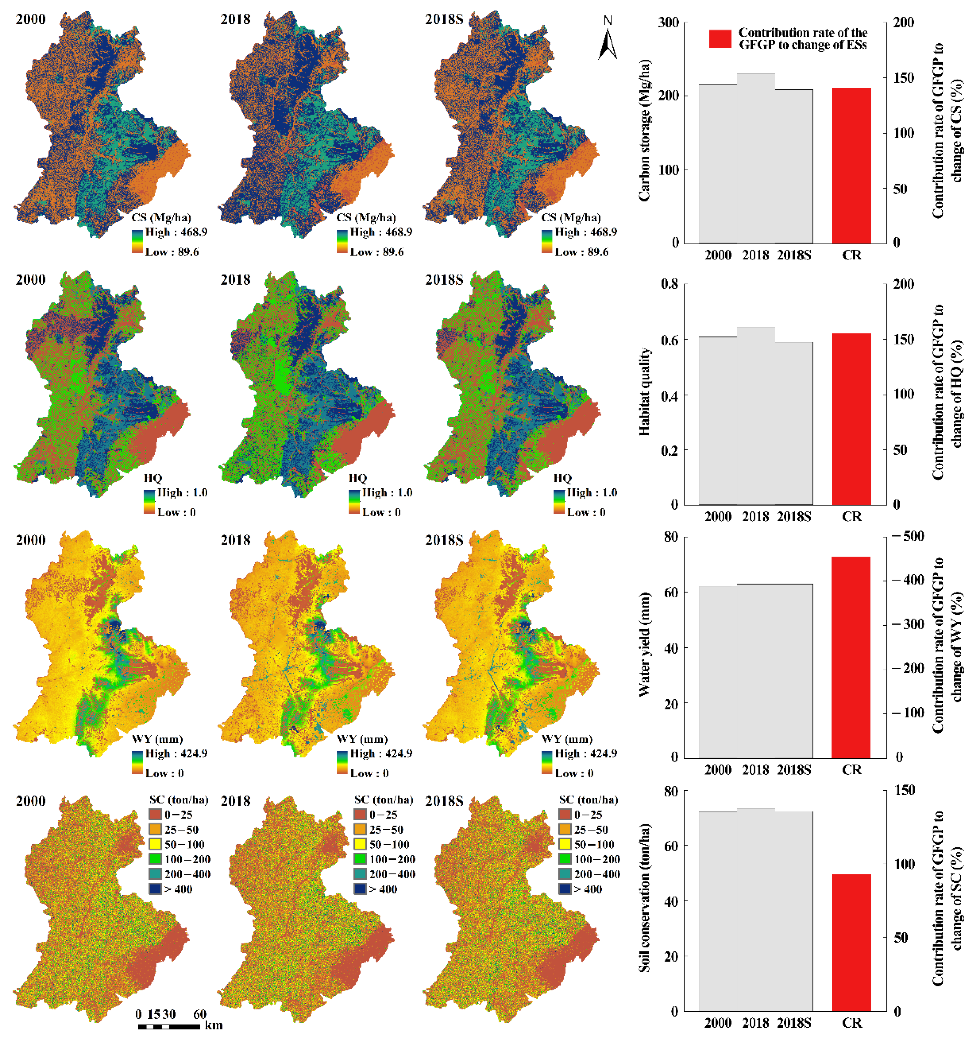
Figure 2 shows the land use patterns in 2000, 2018, and 2018S (the scenario if the GFGP were not implemented). Compared with 2000, the area of farmland decreased by 28.90% in 2018, and the area of construction land, forest, grassland, and shrub land increased by 259.31%, 13.7%, 23.98%, and 4.51%, respectively (Table 3). The area of farmland and forest under the 2018S scenario decreased by 5.21% and 10.92%, respectively, and the area of grassland and shrub land increased by 4.20% and 0.87%, respectively (Table 3). Our results show that the GFGP led to a decrease of 23.69% in the area of farmland, and an increase of 24.62%, 19.78%, and 3.64% in the area of forest, grassland, and shrub land, respectively (Table 3), and thus was the main driving force for the significant increase in regional vegetation cover.

3.2. ESs Change

Figure 3 shows the spatial pattern of ESs in 2000, 2018, and 2018S (the scenario if the GFGP were not implemented). The spatial pattern of CS is consistent with land use, and high-value areas are distributed in mountainous regions with higher forest cover (Figure 3). Compared with 2000, the average CS in 2018 and 2018S increased by 15.47 (Mg/ha) and decreased by 6.33 (Mg/ha), respectively. During the study period, the contribution rate of the GFGP to CS changes was 140.92% (Figure 3). The central and eastern areas are dominated by forest and grassland, with high HQ, while in the western loess hilly region and the southeastern plains, HQ is relatively low (Figure 3). Compared with 2000, the average HQ in 2018 and 2018S increased by 0.035 and decreased by 0.019, respectively. During the study period, the contribution rate of the GFGP to HQ changes was 155.59% (Figure 3). WY was high in the center of the study area and low in the outer regions (Figure 3). Compared with 2000, the average WY in 2018 and 2018S increased by 0.79 (mm) and 4.36 (mm), respectively. During the study period, the GFGP had a significant negative impact on WY, with a contribution rate of −454.48% (Figure 3). The central and eastern regions had high SC values, while the southeast and western regions had relatively low SC (Figure 3). Compared with 2000, the average SC in 2018 and 2018S increased by 0.947 (ton/ha) and 0.067 (ton/ha), respectively. During the study period, the contribution rate of the GFGP to SC changes was 92.96% (Figure 3). In general, the implementation of the GFGP from 2000 to 2018 compensated for the negative impacts of external environmental pressures on CS and HQ, and significantly improved CS, HQ, and SC; however, this improvement came at the expense of WY.

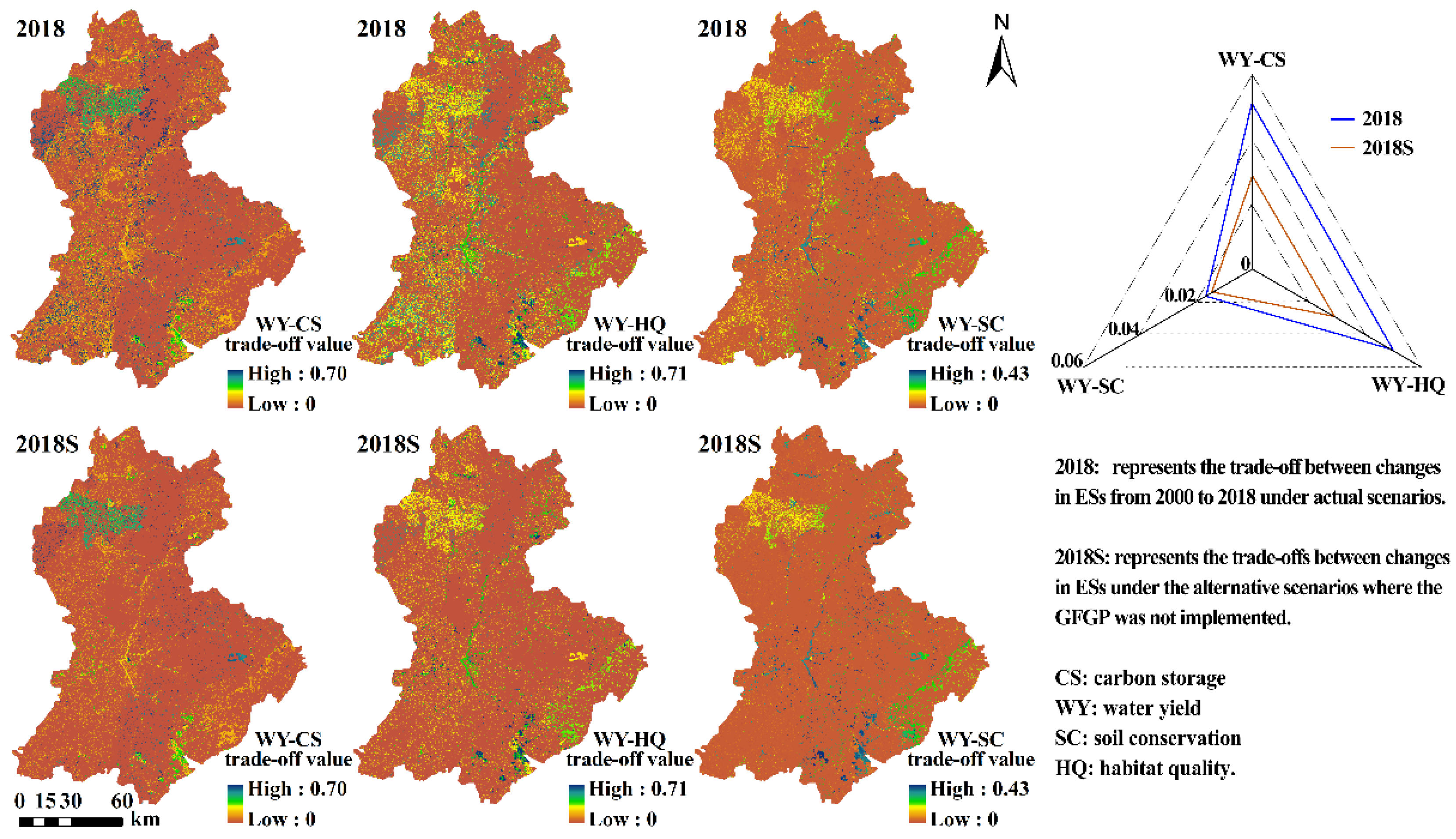
3.3. Trade-Offs Between ESs

The correlation between changes in ESs from 2000 to 2018 and 2018S (the scenarios if the GFGP were not implemented) was analyzed at the sub-watershed scale. CS, HQ, and SC have a significant synergistic relationship, and there is a significant trade-off between these ESs and WY (Table 4). In addition, the correlation coefficients (including positive and negative correlations) between paired ESs in the actual scenario are larger than those in the alternative scenario if the GFGP were not implemented (Table 4). This indicates that the GFGP has intensified the trade-offs and synergies between ESs.
We visualized the WY-CS, WY-HQ, and WY-SC trade-offs using root mean squared error (RMSE), and our results show that the west and southeast are the high value areas of the trade-offs (Figure 4). Average tradeoff values of WY-CS, WY-HQ, and WY-SC are 0.051, 0.050, and 0.016, respectively, in the actual scenario, and the average tradeoff values of WY-CS, WY-HQ, and WY-SC are 0.028, 0.030, and 0.014, respectively, in the alternative scenario if the GFGP were not implemented (Figure 4). This indicates that the implementation of the GFGP strengthens the trade-offs between WY-CS, WY-HQ, and WY-SC.

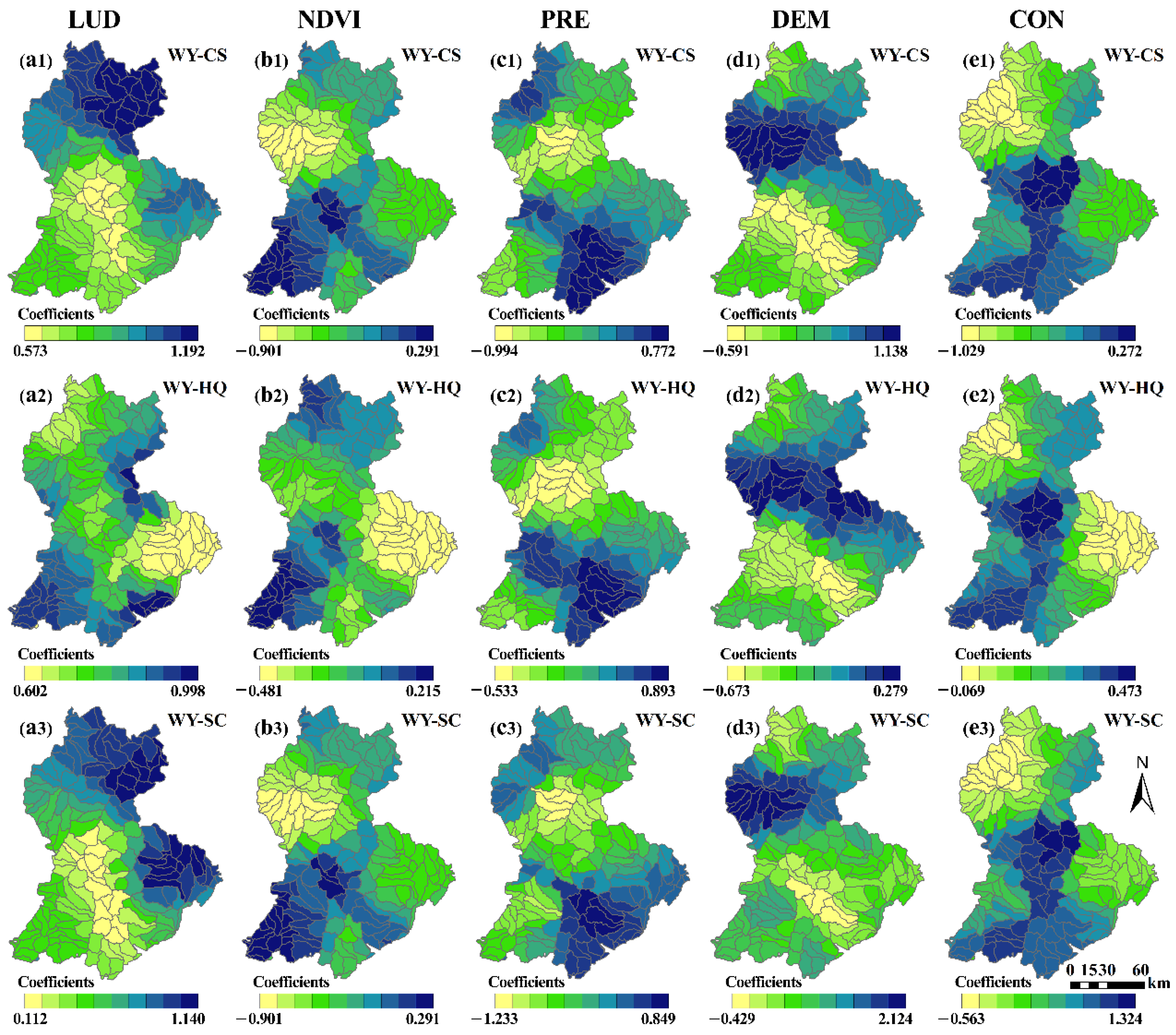
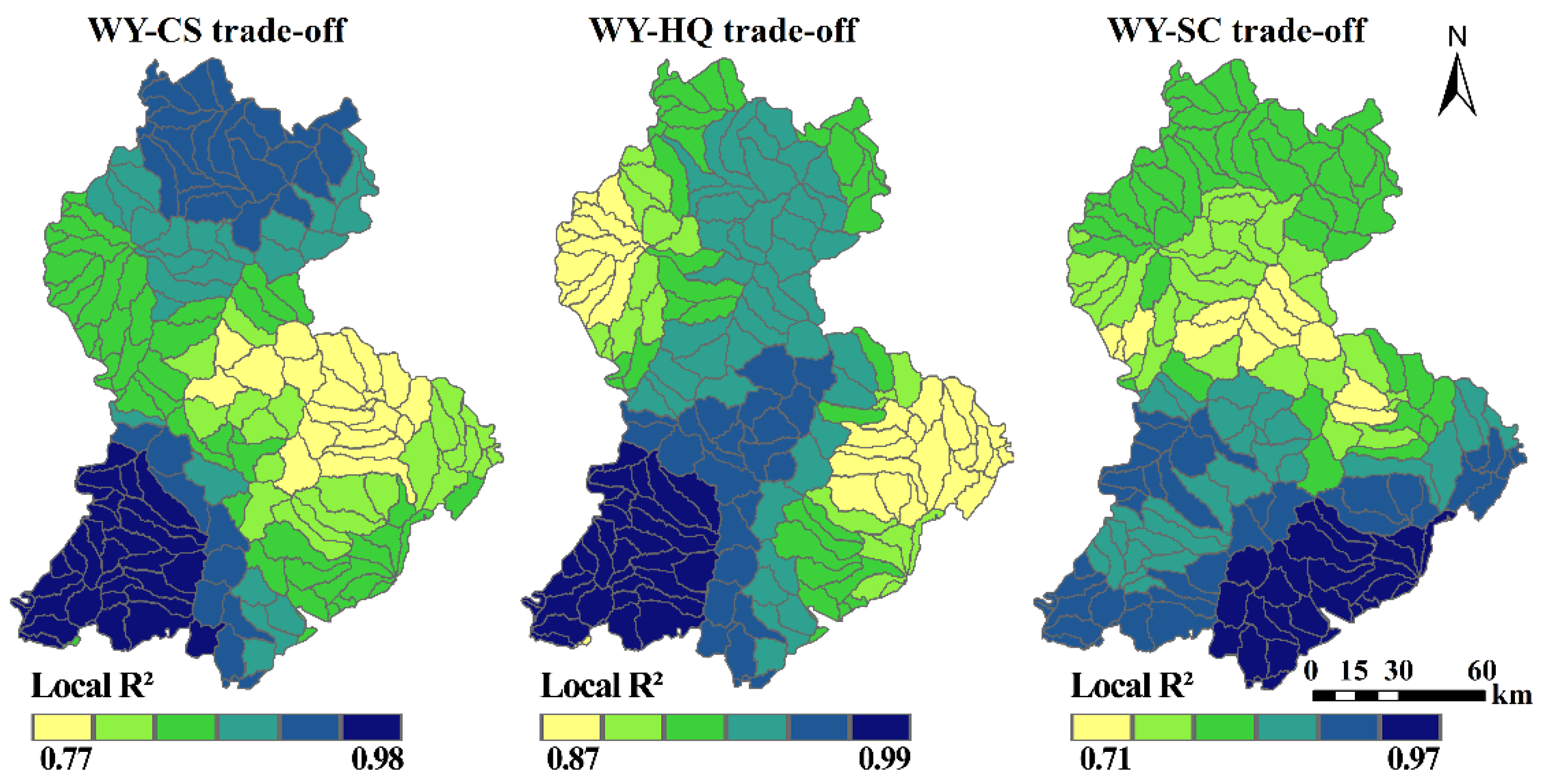
3.4. FACTORS Influencing ESs Trade-Offs

We built a GWR model to explore the geospatial relationship between ES trade-offs and the factors that influence them. Compared with OLS, the adjusted R2 of the GWR model was greater, and the AICc value decreased significantly (Table 5), indicating that the GWR results have higher explanatory power and can more accurately reflect the processes at play.
The correlation coefficient of the GWR model reflects the spatial non-stationary response of ES trade-offs to influencing factors (Figure 5). LUD is significantly positively correlated with WY-CS, WY-HQ, and WY-SC trade-offs, and the correlation coefficient is relatively high in the northeast (Figure 5 (a1–a3), Table 6). NDVI is significantly negatively correlated with WY-CS, WY-HQ, and WY-SC trade-offs, and the correlation coefficient is relatively high in the southwest (Figure 5 (b1–b3), Table 6). PRE is positively correlated with WY-CS and WY-HQ trade-offs, but negatively correlated with the WY-SC trade-off, and the correlation coefficient is high in the southeast (Figure 5 (c1–c3), Table 6). DEM is negatively correlated with the WY-HQ trade-off, but positively correlated with WY-CS and WY-SC trade-offs, and the correlation coefficient is larger in the north (Figure 5 (d1–d3), Table 6). CON is negatively correlated with the WY-CS trade-off, but significantly positively correlated with WY-HQ and WY-SC trade-offs, and the correlation coefficient is larger in the south (Figure 5 (e1–e3), Table 6).
Local R2 maps describe spatial differences in model goodness of fit, ranging between 0 and 1. Our results show that the selected five influencing factors are closely related to ES trade-offs, explaining 90.8%, 94.2%, and 88.2% of the WY-CS, WY-HQ, and WY-SC trade-offs, respectively (Figure 6, Table 5). In general, LUD, CON, and NDVI are the most important driving factors of ES trade-offs, and they are significantly positively correlated with LUD and CON while being negatively correlated with NDVI (Figure 6, Table 6). This means that increasing vegetation cover, controlling the intensity of land use change, and optimizing the development of urbanization are effective ways to alleviate the trade-offs between ESs and realize the synergistic promotion of multiple ESs.

4. Discussion

4.1. Effects of the GFGP on ESs

The GFGP is a successful program for coping with environmental degradation and increasing the supply of ESs [31]. Although the quality of the regional ecological environment has been greatly improved [17,62], realizing the coordinated development of multiple ESs is still a key consideration in optimizing GFGP policies. Our results show that the implementation of the GFGP significantly increased forest, grassland, and shrub land area (Table 3), and vegetation cover increased significantly [24], leading to significant increases in CS, HQ, and SC. This indicates that the GFGP promoted the synergistic relationship among CS, HQ, and SC. However, CS and HQ, under an alternative scenario where the GFGP was not implemented, significantly decreased (Figure 3), indicating that the GFGP effectively compensated for the negative impacts of external environmental pressures on CS and HQ. By comparing the actual scenario in 2018 with the alternative scenario, we found that the GFGP is the most important driving force for the increase in SC, with a contribution rate of 92.96% (Figure 3). In addition, our results show that the GFGP has had a significant negative impact on WY, with a contribution rate of −454.48% (Figure 3). This is mainly due to the large-scale planting of non-native vegetation, which leads to a significant increase in water consumption and evapotranspiration [27,63]. Our research confirms that the GFGP produces significant ecological benefits while also exacerbating regional water resource conflicts, which is consistent with previous studies [26,27,51,64]. However, unlike previous studies, we quantified the contribution rate of the GFGP to ES changes and the impact on the trade-offs/synergies between ESs, providing a more direct reference for alleviating regional water resource conflicts and realizing the synergistic promotion of multiple ESs.

4.2. Suggestions on the Inclusiveness and Sustainable Development of the GFGP

Identifying the dominant factors influencing the trade-offs between ESs is critical to formulating an inclusive and sustainable plan for the GFGP. There are obvious spatial differences in the relationships between ES trade-offs and their influencing factors [65,66], and classical global regression models did not fully reflect the relationships between the two in geographic space [59]. The local coefficients obtained by the GWR model by minimizing the residuals reflect the spatial non-stationary relationships between them [56], effectively overcoming the problems with classic regression models. We used the GWR model to explore the spatially non-stationary relationship between ES trade-offs and their influencing factors, and our results show that LUD, CON, and NDVI are the most important driving factors for ES trade-offs (Figure 5, Table 6). The WY–CS, WY–HQ, and WY–SC trade-offs were significantly positively correlated with LUD and CON, but negatively correlated with NDVI (Figure 5 (a1–a3, b1–b3, e1–e3), Table 6).
Land use change and urbanization are the main drivers of declines in CS, HQ, and SC [57,67], and also have negative impacts on the water conservation capacity of ecosystems [68]. However, land use change and urbanization also reduced the evapotranspiration of surface vegetation to a certain degree [69], and their impacts on precipitation at smaller timescales are also limited [70]. Therefore, increases in LUD and CON intensify the trade-offs between WY–CS, WY–HQ, and WY–SC. NDVI is the most direct manifestation of the effectiveness of afforestation [71]. The GFGP is the main driver of the increase in regional NDVI [24], which not only improves CS, HQ, and SC but also improves the water conservation capacity of the ecosystem [72,73]. Therefore, increasing NDVI helps to alleviate the trade-offs between WY–CS, WY–HQ, and WY–SC.
The correlation coefficient of the GWR model reflects the spatial non-stationary response of ES trade-offs to their influencing factors (Figure 5). In the northeast and south of the study area, urbanization developed rapidly and the intensity of human activity was high (Figure 2), so the correlation coefficient between LUD, CON, and ES trade-offs was relatively large (Figure 5 (a1–a3, e1–e3)). In the southwestern region, the terrain is rugged and vegetation is relatively scarce [34], so the correlation coefficient between NDVI and ESs trade-offs is relatively high (Figure 5 (b1–b3)). Therefore, controlling LUD and CON in the northeast and south, and increasing vegetation cover in the southwest, is essential to alleviate the WY–CS, WY–HQ, and WY–SC trade-offs.
In summary, we propose that future engineering projects should take into account the geospatial relationships between ES trade-offs and their influencing factors. By controlling the intensity of land use change, optimizing the development of urbanization, and improving the effectiveness of afforestation, the inclusive and sustainable development of the regional GFGP can be realized.

4.3. Uncertainties and Limitations

Our research provides a direct and flexible method to quantify the impacts of the GFGP on ESs, but it still has certain limitations. First, changing ESs is a complex process driven by factors such as nature, human activities, and climate change [17,74]. It is very difficult to completely quantify the impact of the GFGP on ESs. Our study used the average climate parameters from 2000 to 2018. Although this method is widely adopted [45,46], climate change during the research period will certainly have had an impact on ESs. Second, the input parameters of the model evaluation are taken from previous studies, but due to the limitations of our data sources, quality, and availability, we did not verify the results of the ES evaluations. Third, because of the limited availability of data, we had to ignore some details of the GFGP, such as tree species selection and configuration, vegetation management methods, etc., although these practices certainly could have a strong impact on ESs [71]. These problems may introduce some uncertainty into our model results. Therefore, it is necessary to obtain long-term positioning observation data and conduct more detailed research on the impacts of the GFGP.

5. Conclusions

Based on scenario analysis, we quantified the impacts of the GFGP on changes in ESs in Lvliang City, a typical ecologically fragile area, and analyzed the main forces driving ES trade-offs through spatial regression. Our research shows that the GFGP compensated for the negative impacts of external environmental pressures on CS and HQ, and significantly improved CS, HQ, and soil conservation (SC), but this improvement came at the expense of water yield (WY). While the GFGP promotes the synergistic development of CS, HQ, and SC, it also intensifies the trade-off relationships between these services and WY. Land use change and urbanization are significantly positively correlated with the trade-offs between WY–CS, WY–HQ, and WY–SC, while increasing NDVI helped to alleviate these trade-offs. Therefore, controlling the intensity of land use change, optimizing the development of urbanization, and improving the effectiveness of afforestation are effective ways to realize the inclusive and sustainable development of the GFGP. The general methods used in this study to quantify the impacts of ecological engineering on ESs can provide a reference for future ecological restoration plans and decision-making in China and around the world.

Supplementary Materials

The following are available online at https://www.mdpi.com/article/10.3390/rs13193966/s1, Table S1: Threats and their maximum distance of influence and weights. Table S2: The sensitivity of habitat types to each threat. Table S3: Table of biophysical coefficients for InVEST. Table S4: Description of variables selected in this study. Table S5: Multicollinearity test among influencing factors.

Author Contributions

Conceptualization, Methodology, and Writing—original draft, B.H.; Formal analysis, Z.Z.; Validation and Resources, H.H.; Software and Data curation, Z.L.; Project administration, X.C.; Supervision, F.K.; Visualization, H.W. All authors have read and agreed to the published version of the manuscript.

Funding

This research was supported by the National Key Research and Development Program of China (No. 2019YFA0607304).

Institutional Review Board Statement

Not applicable.

Informed Consent Statement

Not applicable.

Data Availability Statement

Publicly available datasets were analyzed in this study. Data sources and access links are detailed in Table 1 and Table S4.

Acknowledgments

We sincerely thank the reviewers and editors for their efforts to improve the quality of our paper. We would like to express our gratitude to those who participated in the manuscript revisions.

Conflicts of Interest

The authors declare no conflict of interest.

References

  1. Costanza, R.; d’Arge, R.; De Groot, R.; Farber, S.; Grasso, M.; Hannon, B.; Limburg, K.; Naeem, S.; O’Neill, R.V.; Paruelo, J.; et al. The value of the world’s ecosystem services and natural capital. Nature 1997, 387, 253–260. [Google Scholar] [CrossRef]
  2. Carpenter, S.R.; Mooney, H.A.; Agard, J.; Capistrano, D.; Defries, R.S.; Díaz, S.; Dietz, T.; Duraiappah, A.K.; Oteng-Yeboah, A.; Pereira, H.M.; et al. Science for managing ecosystem services: Beyond the millennium ecosystem assessment. Proc. Natl. Acad. Sci. USA 2009, 106, 1305–1312. [Google Scholar] [CrossRef] [PubMed] [Green Version]
  3. Costanza, R.; De Groot, R.; Sutton, P.; van der Ploeg, S.; Anderson, S.J.; Kubiszewski, I.; Farber, S.; Turner, R.K. Changes in the global value of ecosystem services. Glob. Environ. Chang. 2014, 26, 152–158. [Google Scholar] [CrossRef]
  4. Xiang, H.; Wang, Z.; Mao, D.; Zhang, J.; Zhao, D.; Zeng, Y.; Wu, F. Surface mining caused multiple ecosystem service losses in China. J. Environ. Manag. 2021, 290, 112618. [Google Scholar] [CrossRef] [PubMed]
  5. Newbold, T.; Hudson, L.N.; Hill, S.L.L.; Contu, S.; Lysenko, I.; Senior, R.A.; Börger, L.; Bennett, D.J.; Choimes, A.; Collen, B.; et al. Global effects of land use on local terrestrial biodiversity. Nature 2015, 520, 45–50. [Google Scholar] [CrossRef] [Green Version]
  6. Wunder, S.; Brouwer, R.; Engel, S.; Ezzine-de-Blas, D.; Muradian, R.; Pascual, U.; Pinto, R. From principles to practice in paying for nature’s services. Nat. Sustain. 2018, 1, 145–150. [Google Scholar] [CrossRef]
  7. Zeng, J.; Chen, T.; Yao, X.; Chen, W. Do protected areas improve ecosystem services? A case study of Hoh Xil Nature Reserve in Qinghai-Tibetan Plateau. Remote Sens. 2020, 12, 471. [Google Scholar] [CrossRef] [Green Version]
  8. Benayas, J.M.R.; Newton, A.C.; Diaz, A.; Bullock, J.M. Enhancement of biodiversity and ecosystem services by ecological restoration: A meta-analysis. Science 2009, 325, 1121–1124. [Google Scholar] [CrossRef]
  9. Salzman, J.; Bennett, G.; Carroll, N.; Goldstein, A.; Jenkins, M. The global status and trends of Payments for Ecosystem Services. Nat. Sustain. 2018, 1, 136–144. [Google Scholar] [CrossRef]
  10. Costanza, R.; De Groot, R.; Braat, L.; Kubiszewski, I.; Fioramonti, L.; Sutton, P.; Farber, S.; Grasso, M. Twenty years of ecosystem services: How far have we come and how far do we still need to go? Ecosyst. Serv. 2017, 28, 1–16. [Google Scholar] [CrossRef]
  11. Gao, J. Editorial for the Special Issue “Ecosystem Services with Remote Sensing”. Remote Sens. 2020, 12, 2191. [Google Scholar] [CrossRef]
  12. Turkelboom, F.; Leone, M.; Jacobs, S.; Kelemen, E.; García-Llorente, M.; Baró, F.; Termansen, M.; Barton, D.N.; Berry, P.; Stange, E.; et al. When we cannot have it all: Ecosystem services trade-offs in the context of spatial planning. Ecosyst. Serv. 2018, 29, 566–578. [Google Scholar] [CrossRef]
  13. Qian, D.; Du, Y.; Li, Q.; Guo, X.; Cao, G. Alpine grassland management based on ecosystem service relationships on the southern slopes of the Qilian Mountains, China. J. Environ. Manag. 2021, 288, 112447. [Google Scholar] [CrossRef] [PubMed]
  14. Li, S.; Zhang, Y.; Wang, Z.; Li, L. Mapping human influence intensity in the Tibetan Plateau for conservation of ecological service functions. Ecosyst. Serv. 2018, 30, 276–286. [Google Scholar] [CrossRef]
  15. Schirpke, U.; Tscholl, S.; Tasser, E. Spatio-temporal changes in ecosystem service values: Effects of land-use changes from past to future (1860–2100). J. Environ. Manag. 2020, 272, 111068. [Google Scholar] [CrossRef]
  16. Grafius, D.R.; Corstanje, R.; Warren, P.H.; Evans, K.L.; Hancock, S.; Harris, J.A. The impact of land use/land cover scale on modelling urban ecosystem services. Landsc. Ecol. 2016, 31, 1509–1522. [Google Scholar] [CrossRef] [Green Version]
  17. Liu, Y.; Lü, Y.; Fu, B.; Harris, P.; Wu, L. Quantifying the spatio-temporal drivers of planned vegetation restoration on ecosystem services at a regional scale. Sci. Total. Environ. 2019, 650, 1029–1040. [Google Scholar] [CrossRef]
  18. Zheng, H.; Li, Y.; Robinson, B.E.; Liu, G.; Ma, D.; Wang, F.; Lu, F.; Ouyang, Z.; Daily, G.C. Using ecosystem service trade-offs to inform water conservation policies and management practices. Front. Ecol. Environ. 2016, 14, 527–532. [Google Scholar] [CrossRef]
  19. Feng, Q.; Zhao, W.; Hu, X.; Liu, Y.; Daryanto, S.; Cherubini, F. Trading-off ecosystem services for better ecological restoration: A case study in the Loess Plateau of China. J. Clean. Prod. 2020, 257, 120469. [Google Scholar] [CrossRef]
  20. Divinsky, I.; Becker, N.; Kutiel, P. Ecosystem service tradeoff between grazing intensity and other services-A case study in Karei-Deshe experimental cattle range in northern Israel. Ecosyst. Serv. 2017, 24, 16–27. [Google Scholar] [CrossRef]
  21. Peng, J.; Hu, X.; Wang, X.; Meersmans, J.; Liu, Y.; Qiu, S. Simulating the impact of Grain-for-Green Programme on ecosystem services trade-offs in Northwestern Yunnan, China. Ecosyst. Serv. 2019, 39, 100998. [Google Scholar] [CrossRef]
  22. Cai, W.; Borlace, S.; Lengaigne, M.; Rensch, P.V.; Collins, M.; Vecchi, G.; Timmermann, A.; Santoso, A.; McPhaden, M.J.; Wu, L.; et al. Increasing frequency of extreme El Niño events due to greenhouse warming. Nat. Clim. Chang. 2014, 4, 111–116. [Google Scholar] [CrossRef] [Green Version]
  23. Geng, Q.; Ren, Q.; Yan, H.; Li, L.; Zhao, X.; Mu, X.; Wu, P.; Yu, Q. Target areas for harmonizing the Grain for Green Programme in China’s Loess Plateau. Land Degrad. Dev. 2019, 31, 325–333. [Google Scholar] [CrossRef]
  24. Zheng, K.; Wei, J.; Pei, J.; Cheng, H.; Zhang, X.; Huang, F.; Li, F.; Ye, J. Impacts of climate change and human activities on grassland vegetation variation in the Chinese Loess Plateau. Sci. Total. Environ. 2019, 660, 236–244. [Google Scholar] [CrossRef]
  25. Hou, Y.; Lü, Y.; Chen, W.; Fu, B. Temporal variation and spatial scale dependency of ecosystem service interactions: A case study on the central Loess Plateau of China. Landsc. Ecol. 2017, 32, 1201–1217. [Google Scholar] [CrossRef]
  26. Wen, X.; Théau, J. Spatiotemporal analysis of water-related ecosystem services under ecological restoration scenarios: A case study in northern Shaanxi, China. Sci. Total. Environ. 2020, 720, 137477. [Google Scholar] [CrossRef] [PubMed]
  27. Feng, X.; Fu, B.; Piao, S.; Wang, S.; Ciais, P.; Zeng, Z.; Lü, Y.; Zeng, Y.; Li, Y.; Jiang, X.; et al. Revegetation in China’s Loess Plateau is approaching sustainable water resource limits. Nat. Clim. Chang. 2016, 6, 1019–1022. [Google Scholar] [CrossRef]
  28. Chen, Y.; Wang, K.; Lin, Y.; Shi, W.; Song, Y.; He, X. Balancing green and grain trade. Nat. Geosci. 2015, 8, 739–741. [Google Scholar] [CrossRef]
  29. Yang, S.; Bai, Y.; Alatalo, J.M.; Wang, H.; Jiang, B.; Liu, G.; Chen, G. Spatio-temporal changes in water-related ecosystem services provision and trade-offs with food production. J. Clean. Prod. 2021, 286, 125316. [Google Scholar] [CrossRef]
  30. Mandle, L.; Shields-Estrada, A.; Chaplin-Kramer, R.; Mitchell, M.G.E.; Bremer, L.L.; Gourevitch, J.D.; Hawthorne, P.; Johnson, J.A.; Robinson, B.E.; Smith, J.R.; et al. Increasing decision relevance of ecosystem service science. Nat. Sustain. 2021, 4, 161–169. [Google Scholar] [CrossRef]
  31. Ouyang, Z.; Zheng, H.; Xiao, Y.; Polasky, S.; Liu, J.; Xu, W.; Wang, Q.; Zhang, L.; Xiao, Y.; Rao, E.; et al. Improvements in ecosystem services from investments in natural capital. Science 2016, 352, 1455–1459. [Google Scholar] [CrossRef]
  32. Yang, S.; Zhao, W.; Liu, Y.; Wang, S.; Wang, J.; Zhai, R. Influence of land use change on the ecosystem service trade-offs in the ecological restoration area: Dynamics and scenarios in the Yanhe watershed, China. Sci. Total. Environ. 2018, 644, 556–566. [Google Scholar] [CrossRef]
  33. Peng, J.; Tian, L.; Zhang, Z.; Zhao, Y.; Green, S.M.; Quine, T.A.; Liu, H.; Meersmans, J. Distinguishing the impacts of land use and climate change on ecosystem services in a karst landscape in China. Ecosyst. Serv. 2020, 46, 101199. [Google Scholar] [CrossRef]
  34. Sun, C.; Li, X.; Zhang, W.; Chen, W.; Wang, J. Evaluation of ecological security in poverty-stricken region of Lüliang Mountain based on the remote sensing image. China Environ. Sci. 2019, 39, 5352–5360. [Google Scholar]
  35. Li, J.; Wang, Y. Spatial coupling characteristics of eco-environment quality and economic poverty in Lüliang area. Chin. J. Appl. Ecol. 2014, 25, 1715–1724. [Google Scholar]
  36. Sharp, R.; Tallis, H.T.; Ricketts, T.; Guerry, A.D.; Wood, S.A.; Chaplin-Kramer, R.; Nelson, E.; Ennaanay, D.; Wolny, S.; Olwero, N.; et al. InVEST 3.8.0 User’s Guide. The Natural Capital Project: Stanford University, University of Minnesota, The Nature Conservancy, and World Wildlife Fund. 2020. Available online: http://releases.naturalcapitalproject.org/invest-userguide/latest/#supporting-tools (accessed on 26 November 2020).
  37. Zhang, L.; Fu, B.; Lü, Y.; Zeng, Y. Balancing multiple ecosystem services in conservation priority setting. Landsc. Ecol. 2015, 30, 535–546. [Google Scholar] [CrossRef]
  38. Liu, L.; Zhang, H.; Gao, Y.; Zhu, W.; Liu, X.; Xu, Q. Hotspot identification and interaction analyses of the provisioning of multiple ecosystem services: Case study of Shaanxi Province, China. Ecol. Indic. 2019, 107, 105566. [Google Scholar] [CrossRef]
  39. Sun, X.; Lu, Z.; Li, F.; Crittenden, J.C. Analyzing spatio-temporal changes and trade-offs to support the supply of multiple ecosystem services in Beijing, China. Ecol. Indic. 2018, 94, 117–129. [Google Scholar] [CrossRef]
  40. Liu, C.; Wang, C. Spatio-temporal evolution characteristics of habitat quality in the Loess Hilly Region based on land use change: A case study in Yuzhong county. Acta Ecol. Sin. 2018, 38, 7300–7311. [Google Scholar]
  41. Zhou, L.; Tang, J.; Liu, X.; Dang, X.; Mu, H. Effects of urban expansion on habitat quality in densely populated areas on the Loess Plateau: A case study of Lanzhou, Xi’an-Xianyang and Taiyuan, China. Chin. J. Appl. Ecol. 2021, 32, 261–270. [Google Scholar]
  42. Liang, Y.; Hashimoto, S.; Liu, L. Integrated assessment of land-use/land-cover dynamics on carbon storage services in the Loess Plateau of China from 1995 to 2050. Ecol. Indic. 2021, 120, 106939. [Google Scholar] [CrossRef]
  43. Zhang, Y.; Shi, X.; Tang, Q. Carbon storage assessment in the upper reaches of the Fenhe River under different land use scenarios. Acta Ecol. Sin. 2021, 41, 360–373. [Google Scholar]
  44. Tang, X.; Zhao, X.; Bai, Y.; Tang, Z.; Wang, W.; Zhao, Y.; Wan, H.; Xie, Z.; Shi, X.; Wu, B.; et al. Carbon pools in China’s terrestrial ecosystems: New estimates based on an intensive field survey. Proc. Natl. Acad. Sci. USA 2018, 115, 4021–4026. [Google Scholar] [CrossRef] [PubMed] [Green Version]
  45. Zheng, H.; Wang, L.; Peng, W.; Zhang, C.; Li, C.; Robinson, B.E.; Wu, X.; Kong, L.; Li, R.; Xiao, Y.; et al. Realizing the values of natural capital for inclusive, sustainable development: Informing China’s new ecological development strategy. Proc. Natl. Acad. Sci. USA 2019, 116, 8623–8628. [Google Scholar] [CrossRef] [Green Version]
  46. Fu, Q.; Li, B.; Hou, Y.; Bi, X.; Zhang, X. Effects of land use and climate change on ecosystem services in Central Asia’s arid regions: A case study in Altay Prefecture, China. Sci. Total. Environ. 2017, 607, 633–646. [Google Scholar] [CrossRef] [PubMed]
  47. Bradford, J.B.; D’Amato, A.W. Recognizing trade-offs in multi-objective land management. Front. Ecol. Environ. 2012, 10, 210–216. [Google Scholar] [CrossRef] [Green Version]
  48. Lu, N.; Fu, B.; Jin, T.; Chang, R. Trade-off analyses of multiple ecosystem services by plantations along a precipitation gradient across Loess Plateau landscapes. Landsc. Ecol. 2014, 29, 1697–1708. [Google Scholar] [CrossRef]
  49. Xu, J.; Chen, J.; Liu, Y. Partitioned responses of ecosystem services and their tradeoffs to human activities in the Belt and Road region. J. Clean. Prod. 2020, 276, 123205. [Google Scholar]
  50. Luo, Y.; Lü, Y.; Fu, B.; Zhang, Q.; Li, T.; Hu, W.; Comber, A. Half century change of interactions among ecosystem services driven by ecological restoration: Quantification and policy implications at a watershed scale in the Chinese Loess Plateau. Sci. Total. Environ. 2019, 651, 2546–2557. [Google Scholar] [CrossRef] [Green Version]
  51. Fu, B.; Wang, S.; Liu, Y.; Liu, J.; Liang, W.; Miao, C. Hydrogeomorphic ecosystem responses to natural and anthropogenic changes in the Loess Plateau of China. Annu. Rev. Earth Planet. Sci. 2017, 45, 223–243. [Google Scholar] [CrossRef]
  52. Jiang, C.; Zhang, H.; Zhang, Z. Spatially explicit assessment of ecosystem services in China’s Loess Plateau: Patterns, interactions, drivers, and implications. Glob. Planet. Chang. 2018, 161, 41–52. [Google Scholar] [CrossRef]
  53. Wang, L.; Ma, S.; Jiang, J.; Zhao, Y.; Zhang, J. Spatiotemporal Variation in Ecosystem Services and Their Drivers among Different Landscape Heterogeneity Units and Terrain Gradients in the Southern Hill and Mountain Belt, China. Remote Sens. 2021, 13, 1375. [Google Scholar] [CrossRef]
  54. Ahmed, M.A.; Abd-Elrahman, A.; Escobedo, F.J.; Cropper, W.P.; Martin, T.A.; Timilsina, N. Spatially-explicit modeling of multi-scale drivers of aboveground forest biomass and water yield in watersheds of the Southeastern United States. J. Environ. Manag. 2017, 199, 158–171. [Google Scholar] [CrossRef] [PubMed]
  55. Zhang, Z.; Liu, Y.; Wang, Y.; Liu, Y.; Zhang, Y.; Zhang, Y. What factors affect the synergy and tradeoff between ecosystem services, and how, from a geospatial perspective? J. Clean. Prod. 2020, 257, 120454. [Google Scholar] [CrossRef]
  56. Fotheringham, A.S.; Yang, W.; Kang, W. Multiscale geographically weighted regression (MGWR). Ann. Am. Assoc. Geogr. 2017, 107, 1247–1265. [Google Scholar] [CrossRef]
  57. Clerici, N.; Cote-Navarro, F.; Escobedo, F.J.; Rubiano, K.; Villegas, J.C. Spatio-temporal and cumulative effects of land use-land cover and climate change on two ecosystem services in the Colombian Andes. Sci. Total. Environ. 2019, 685, 1181–1192. [Google Scholar] [CrossRef] [PubMed]
  58. Sannigrahi, S.; Zhang, Q.; Pilla, F.; Joshi, P.K.; Basu, B.; Keesstra, S.; Roy, P.S.; Wang, Y.; Sutton, P.C.; Chakraborti, S.; et al. Responses of ecosystem services to natural and anthropogenic forcings: A spatial regression based assessment in the world’s largest mangrove ecosystem. Sci. Total. Environ. 2020, 715, 137004. [Google Scholar] [CrossRef]
  59. Gao, J.; Zuo, L.; Liu, W. Environmental determinants impacting the spatial heterogeneity of karst ecosystem services in Southwest China. Land Degrad. Dev. 2020, 32, 1718–1731. [Google Scholar] [CrossRef]
  60. Li, S.; He, Y.; Xu, H.; Zhu, C.; Dong, B.; Lin, Y.; Si, B.; Deng, J.; Wang, K. Impacts of Urban Expansion Forms on Ecosystem Services in Urban Agglomerations: A Case Study of Shanghai-Hangzhou Bay Urban Agglomeration. Remote Sens. 2021, 13, 1908. [Google Scholar] [CrossRef]
  61. Li, B.; Wang, W. Trade-offs and synergies in ecosystem services for the Yinchuan Basin in China. Ecol. Indic. 2018, 84, 837–846. [Google Scholar] [CrossRef]
  62. Guo, S.; Han, X.; Li, H.; Wang, T.; Tong, X.; Ren, G.; Feng, Y.; Yang, G. Evaluation of soil quality along two revegetation chronosequences on the Loess Hilly Region of China. Sci. Total. Environ. 2018, 633, 808–815. [Google Scholar] [CrossRef] [PubMed]
  63. Yang, L.; Che, L.; Wei, W.; Yu, Y.; Zhang, H. Comparison of deep soil moisture in two re-vegetation watersheds in semi-arid regions. J. Hydrol. 2014, 513, 314–321. [Google Scholar] [CrossRef]
  64. Jia, X.; Fu, B.; Feng, X.; Hou, G.; Liu, Y.; Wang, X. The tradeoff and synergy between ecosystem services in the Grain-for-Green areas in Northern Shaanxi, China. Ecol. Indic. 2014, 43, 103–113. [Google Scholar] [CrossRef]
  65. García, A.M.; Santé, I.; Loureiro, X.; Miranda, D. Green infrastructure spatial planning considering ecosystem services assessment and trade-off analysis. Application at landscape scale in Galicia region (NW Spain). Ecosyst. Serv. 2020, 43, 101115. [Google Scholar] [CrossRef]
  66. Liang, J.; Li, S.; Li, X.; Li, X.; Liu, Q.; Meng, Q.; Lin, A.; Li, J. Trade-off analyses and optimization of water-related ecosystem services (WRESs) based on land use change in a typical agricultural watershed, southern China. J. Clean. Prod. 2021, 279, 123851. [Google Scholar] [CrossRef]
  67. Wang, X.; Yan, F.; Su, F. Impacts of Urbanization on the Ecosystem Services in the Guangdong-Hong Kong-Macao Greater Bay Area, China. Remote Sens. 2020, 12, 3269. [Google Scholar] [CrossRef]
  68. Zhang, Y.; Liu, Y.; Zhang, Y.; Liu, Y.; Zhang, G.; Chen, Y. On the spatial relationship between ecosystem services and urbanization: A case study in Wuhan, China. Sci. Total. Environ. 2018, 637–638, 780–790. [Google Scholar] [CrossRef]
  69. Gao, J.; Li, F.; Gao, H.; Zhou, C.; Zhang, X. The impact of land-use change on water-related ecosystem services: A study of the Guishui River Basin, Beijing, China. J. Clean. Prod. 2017, 163, S148–S155. [Google Scholar] [CrossRef]
  70. Lang, Y.; Song, W.; Zhang, Y. Responses of the water-yield ecosystem service to climate and land use change in Sancha River Basin, China. Phys. Chem. Earth 2017, 101, 102–111. [Google Scholar] [CrossRef]
  71. Wu, X.; Wang, S.; Fu, B.; Liu, J. Spatial variation and influencing factors of the effectiveness of afforestation in China’s Loess Plateau. Sci. Total. Environ. 2021, 771, 144904. [Google Scholar] [CrossRef]
  72. Wen, X.; Deng, X.; Zhang, F. Scale effects of vegetation restoration on soil and water conservation in a semi-arid region in China: Resources conservation and sustainable management. Resour. Conserv. Recycl. 2019, 151, 104474. [Google Scholar] [CrossRef]
  73. Zhou, G.; Wei, X.; Chen, X.; Zhou, P.; Liu, X.; Xiao, Y.; Sun, G.; Scott, D.F.; Zhou, S.; Han, L.; et al. Global pattern for the effect of climate and land cover on water yield. Nat. Commun. 2015, 6, 5918. [Google Scholar] [CrossRef] [PubMed] [Green Version]
  74. He, Y.; Kuang, Y.; Zhao, Y.; Ruan, Z. Spatial Correlation between Ecosystem Services and Human Disturbances: A Case Study of the Guangdong–Hong Kong–Macao Greater Bay Area, China. Remote Sens. 2021, 13, 1174. [Google Scholar] [CrossRef]
Figure 1. Location and elevation of study area.
Remotesensing 13 03966 g001
Figure 2. Land use patterns in 2000, 2018, and 2018S. 2018S: the scenario if the GFGP were not implemented.
Remotesensing 13 03966 g002
Figure 3. Spatial pattern of ESs in 2000, 2018, and 2018S. 2018S: the scenario if the GFGP were not implemented. The bar chart on the right represents the average value of ESs in 2000, 2018, and 2018S and the contribution rate of the GFGP to the changes in ESs. Abbreviations: CS: carbon storage; WY: water yield; SC: soil conservation; HQ: habitat quality.
Remotesensing 13 03966 g003
Figure 4. The spatial distributions of trade-offs between ESs. The radar graph on the right represents the average values of trade-offs between ESs.
Remotesensing 13 03966 g004
Figure 5. GWR coefficients between ES trade-offs and their influencing factors. Abbreviations: CS: carbon storage; WY: water yield; SC: soil conservation; HQ: habitat quality; LUD: dynamic degree of comprehensive land use change; NDVI: Normalized Difference Vegetation Index; PRE: precipitation; DEM: elevation; CON: percentage of construction land.
Remotesensing 13 03966 g005
Figure 6. Spatial patterns of local R2 from GWR between ES trade-offs and influencing factors. Abbreviations: CS: carbon storage; WY: water yield; SC: soil conservation; HQ: habitat quality.
Remotesensing 13 03966 g006
Table 1. Description and sources of data used to evaluate ESs.
DataData FormatData DescriptionData Sources
Land use mapsRaster
(30 m)
Land use maps interpreted from Landsat TM/ETM/OLI images. Land use types are classified into seven categories: farmland, forest, grassland, shrub land, water body, construction land, and unused land.Data Center for Resources and Environmental Sciences, Chinese Academy of Sciences (http://www.resdc.cn/ (accessed on 16 March 2021))
Digital Elevation ModelRaster
(30 m)
Elevation data.Geospatial Data Cloud (http://www.gscloud.cn (accessed on 16 March 2021))
Meteorological dataRaster
(1 km)
Including monthly average temperature and precipitation, annual average temperature and precipitation, and potential evapotranspiration.National Earth System Science Data Center (http://www.geodata.cn/ (accessed on 16 March 2021))
Soil propertiesRaster
(1 km)
Including soil texture, topsoil sand fraction, topsoil silt fraction, topsoil clay fraction, topsoil organic carbon, root restricting layer depth, and plant available water content.Harmonized World Soil database (http://www.iiasa.ac.at/Research/LUC/External-World-soil-database/HTML/ (accessed on 16 March 2021))
Evapotranspiration coefficient (Kc)Excel formatPlant evapotranspiration for different land use types.Food and Agriculture Organization of the United Nations (FAO) (http://www.fao.org/3/X0490E/x0490e0b.htm (accessed on 16 March 2021))
Watershed boundaryShapefileDigital watershed atlas.HydroSHEDS (http://hydrosheds.org/ (accessed on 16 March 2021))
Table 2. Methods for quantifying ESs.
ESsMethodsMathematical Expression
WYInVEST model water yield module W Y x = ( 1 A E T x / P x ) × P x
WYx: annual water yield for each grid cell; AETx: annual actual evapotranspiration for pixel x; Px: annual precipitation on pixel x; Biophysical coefficients of model input are shown in Table S3.
SCInVEST model sediment delivery ratio module S C = R × K × L S × ( 1 C × P )
SC: soil conservation; R: rainfall erosion factor; K: soil erosion factor; LS: slope length and gradient factor; C: vegetation cover factor; P: support practice factor. R and K are calculated to refer to the method of Yang et al. [32] and Zhang et al. [37]. We assigned C and P values according to existing literature [17,36,39] (Table S3).
HQInVEST model habitat quality module H Q = H j × [ 1 ( D x j Z D x j Z + K Z ) ]
HQ: habitat quality; Hj: habitat suitability for habitat type j; Dxj: degree of habitat degradation in pixel x that is in habitat type j; K: half-saturation constant; Z: default parameter of the normalized constant model.
CSInVEST model carbon module C S = C a + C b + C s + C d
CS: carbon storage; Ca, Cb, Cs, and Cd are carbon densities in aboveground biomass, belowground biomass, soil, and dead matter, respectively, for each land use type.
Table 3. Land use changes from 2000 to 2018 and 2018S. 2018S: the scenario if the GFGP were not implemented.
Land Use TypesFarmlandForestGrasslandShrub LandWater BodyConstruction LandUnused Land
2018Change area (km2)−2515.04527.151214.05140.63−24.39656.970.62
Change ratio (%)−28.90%13.70%23.98%4.51%−17.36%259.31%87.06%
2018SChange area (km2)−453.05−420.01212.6127.23−24.39656.970.64
Change ratio (%)−5.21%−10.92%4.20%0.87%−17.36%259.31%90.36%
Effect of GFGP on land use change (%)−23.69%24.62%19.78%3.64%00−3.30%
Table 4. Pearson’s correlation analysis between changes in ecosystem services.
N = 181CS2018HQ2018SC2018WY2018CS2018SHQ2018SSC2018SWY2018S
CS20181
HQ20180.920 **1
SC20180.835 **0.889 **1
WY2018−0.804 **−0.898 **−0.641 **1
CS2018S 1
HQ2018S 0.684 **1
SC2018S 0.384 **0.397 **1
WY2018S −0.645 **−0.878 **−0.0751
CS2018 (CS2018S), HQ2018 (HQ2018S), SC2018 (SC2018S), and WY2018 (WY2018S), respectively, indicate changes in carbon storage, habitat quality, soil conservation, and water yield in 2018 (scenarios with and without the implementation of the GFGP) relative to 2000; N represents the number of sub-watersheds; ** indicates significance at the p < 0.01 level.
Table 5. Model fit metrics for ordinary least squares (OLS) regression and GWR.
ES Trade-Offs Fit MetricsModel
OLSGWR
WY-CSR2 (adjust)0.8370.908
AICc194.958128.907
WY-HQR2 (adjust)0.9010.942
AICc104.27948.576
WY-SCR2 (adjust)0.7210.882
AICc291.957182.843
Abbreviations: CS: carbon storage; WY: water yield; SC: soil conservation; HQ: habitat quality.
Table 6. Mean statistics of GWR coefficients between ES trade-offs and influencing factors.
ESs Trade-OffsLUDNDVIPREDEMCON
WY-CS0.888−0.0360.0440.070−0.143
WY-HQ0.794−0.0520.120−0.1260.206
WY-SC0.595−0.054−0.0100.4240.619
Abbreviations: CS: carbon storage; WY: water yield; SC: soil conservation; HQ: habitat quality; LUD: dynamic degree of comprehensive land use change; NDVI: Normalized Difference Vegetation Index; PRE: precipitation; DEM: elevation; CON: percentage of construction land.
Publisher’s Note: MDPI stays neutral with regard to jurisdictional claims in published maps and institutional affiliations.

