
Dynamic Assessment of the Impact of Flood Disaster on Economy and Population under Extreme Rainstorm Events


Abstract
:1. Introduction
2. Materials and Methods
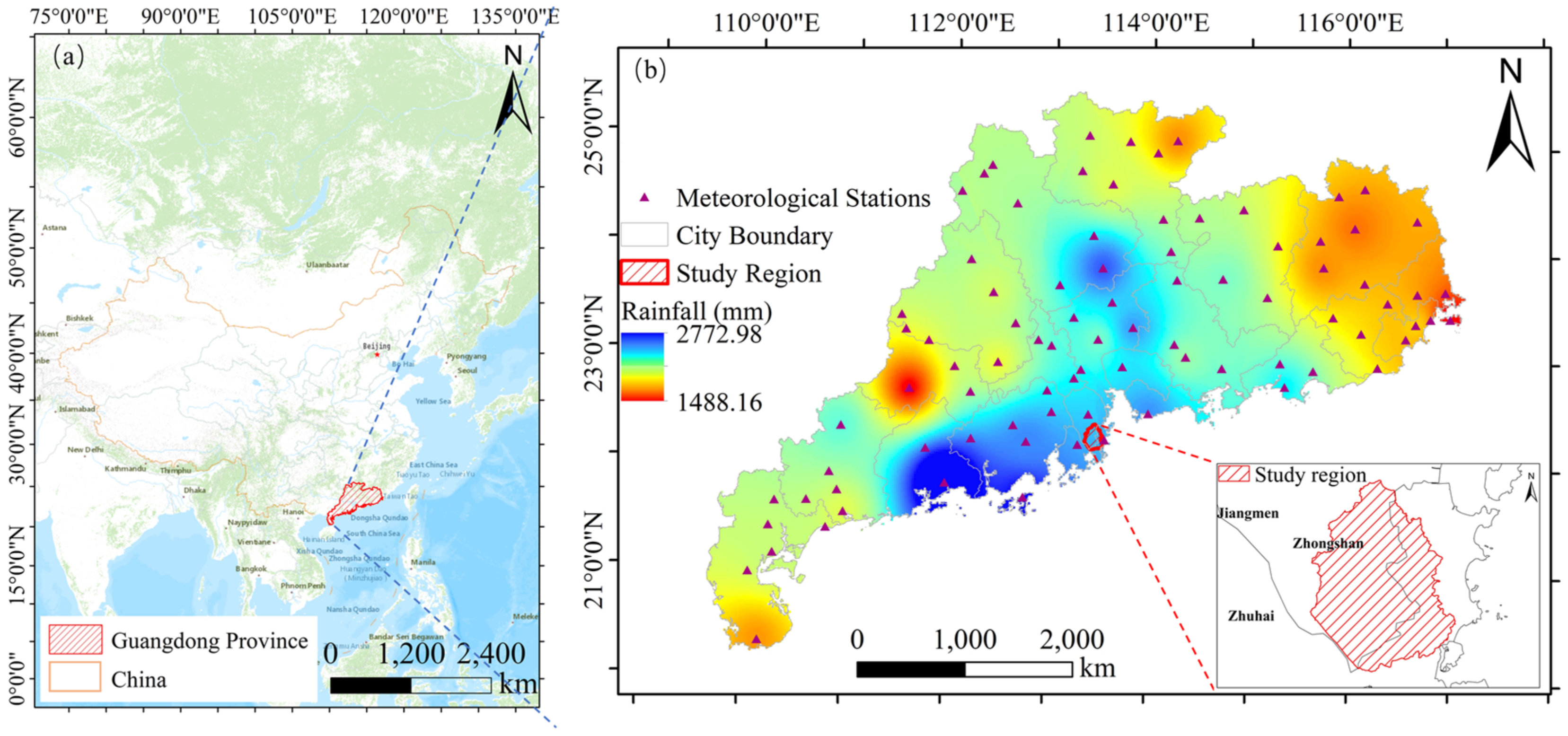
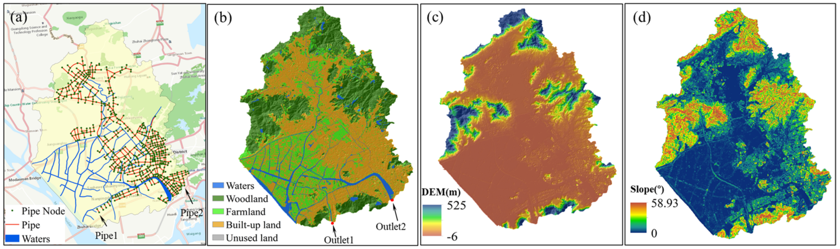
2.1. Study Area
2.2. Data Sources
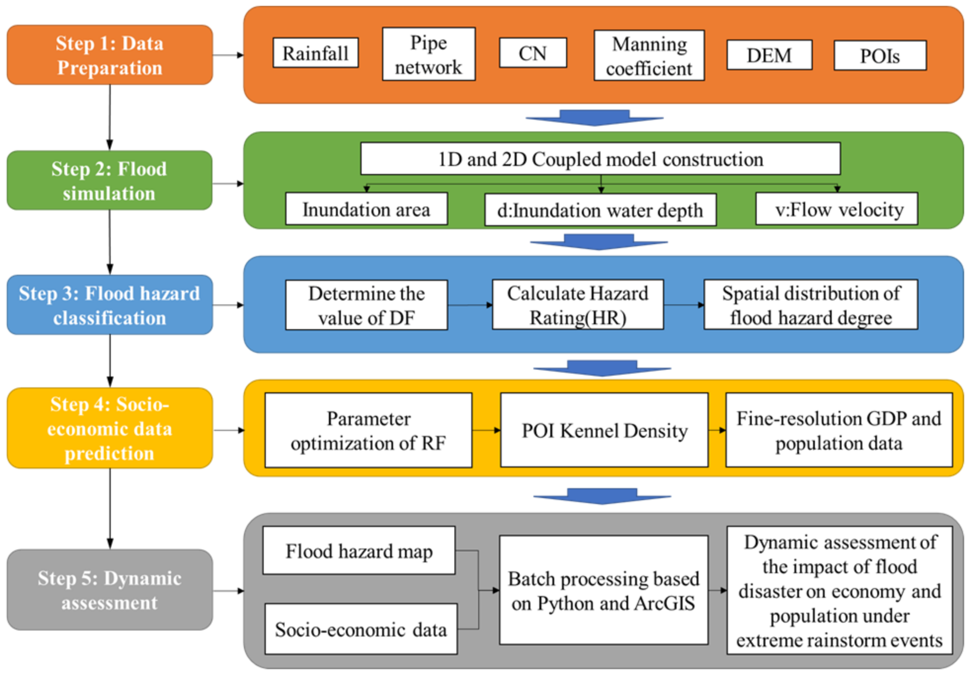
2.3. Methods
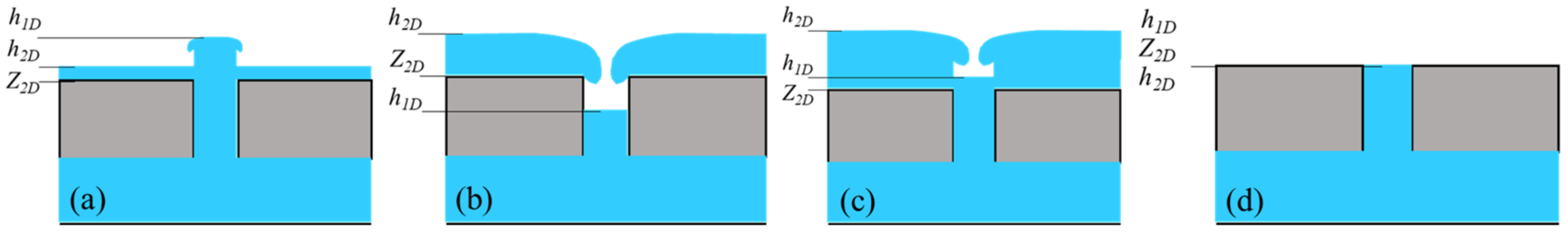
2.3.1. Principle and Method of Urban Flood Hydrodynamic Model
- h2D < h1D, the node water level was higher than the surface water level, the water flowed from the drainage network to the surface;
- h1D < Z2D < h2D, the node water level was lower than the surface elevation, the water flowed from the surface to the drainage network;
- Z2D < h1D < h2D, the node water level was higher than the surface elevation and lower than the surface water level, the water flowed from the surface to the drainage network;
- Z2D = h1D = h2D, the node water level, surface elevation, and surface water level were all equal, and were in a critical state of water exchange. In this case, it was assumed that no water exchange occurred.
2.3.2. Flood Hazard Classification Method
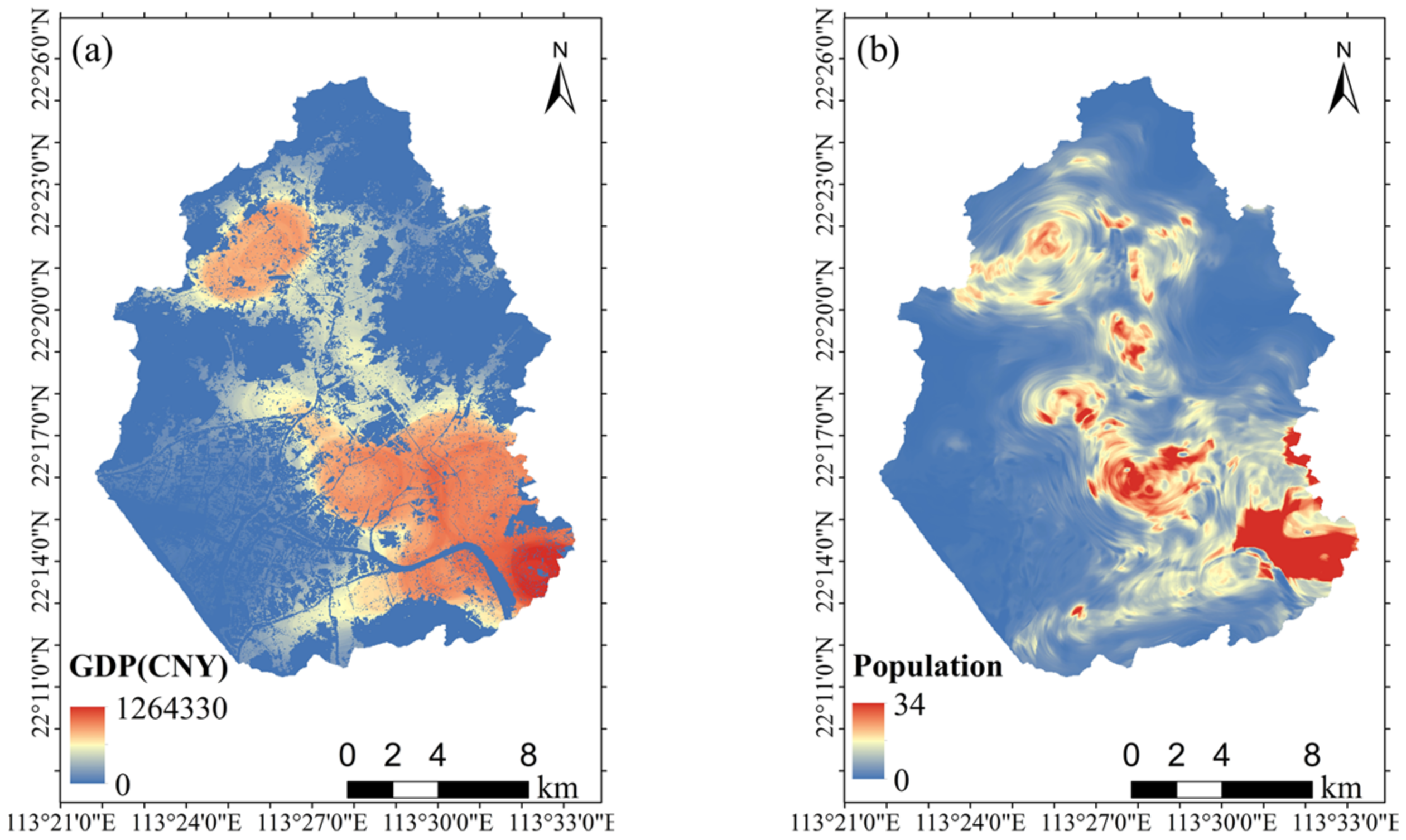
2.3.3. Spatialization Method of Fine-Resolution GDP and Population
2.3.4. Dynamic Assessment Method
3. Results
3.1. Urban Flood Simulation Results
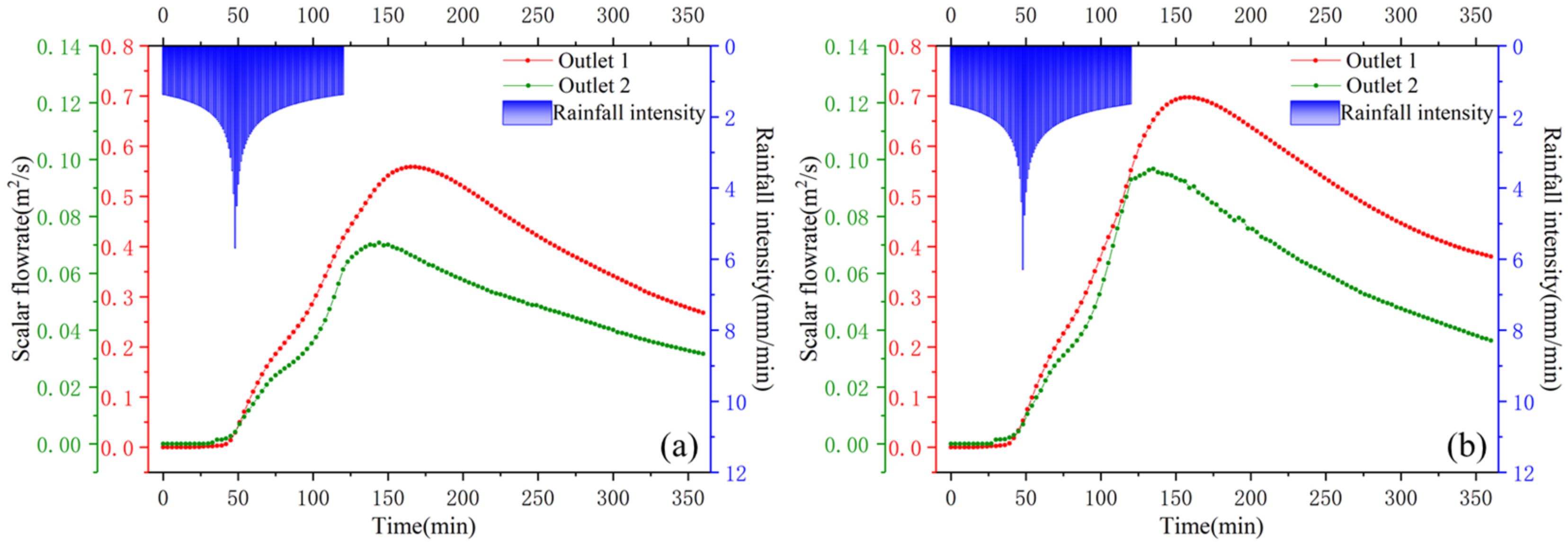
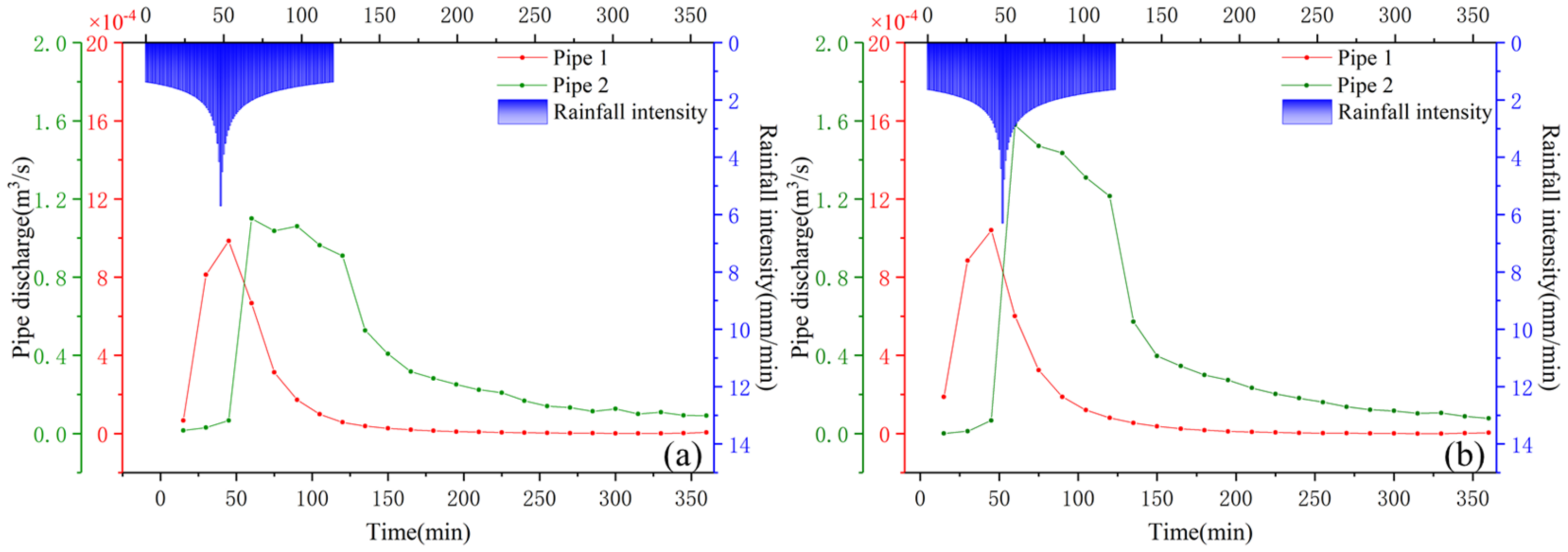
3.1.1. Model Rationality Verification
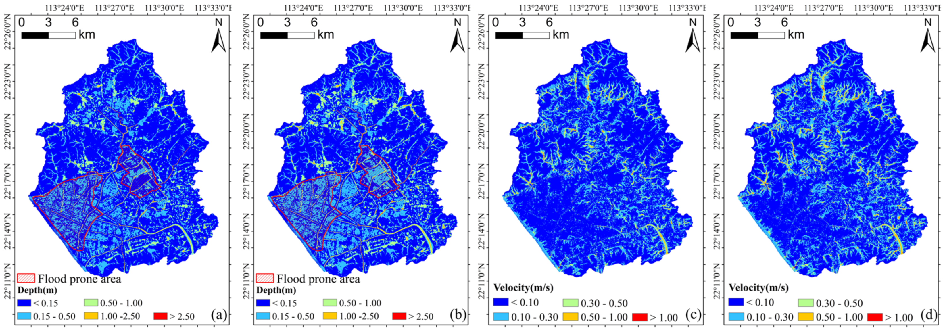
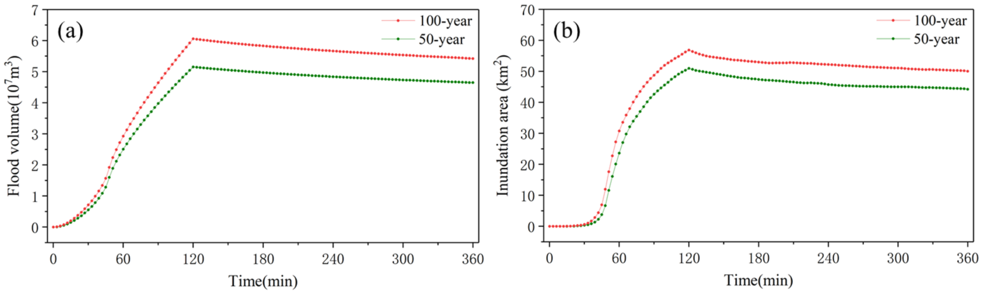
3.1.2. Flood Simulation Results
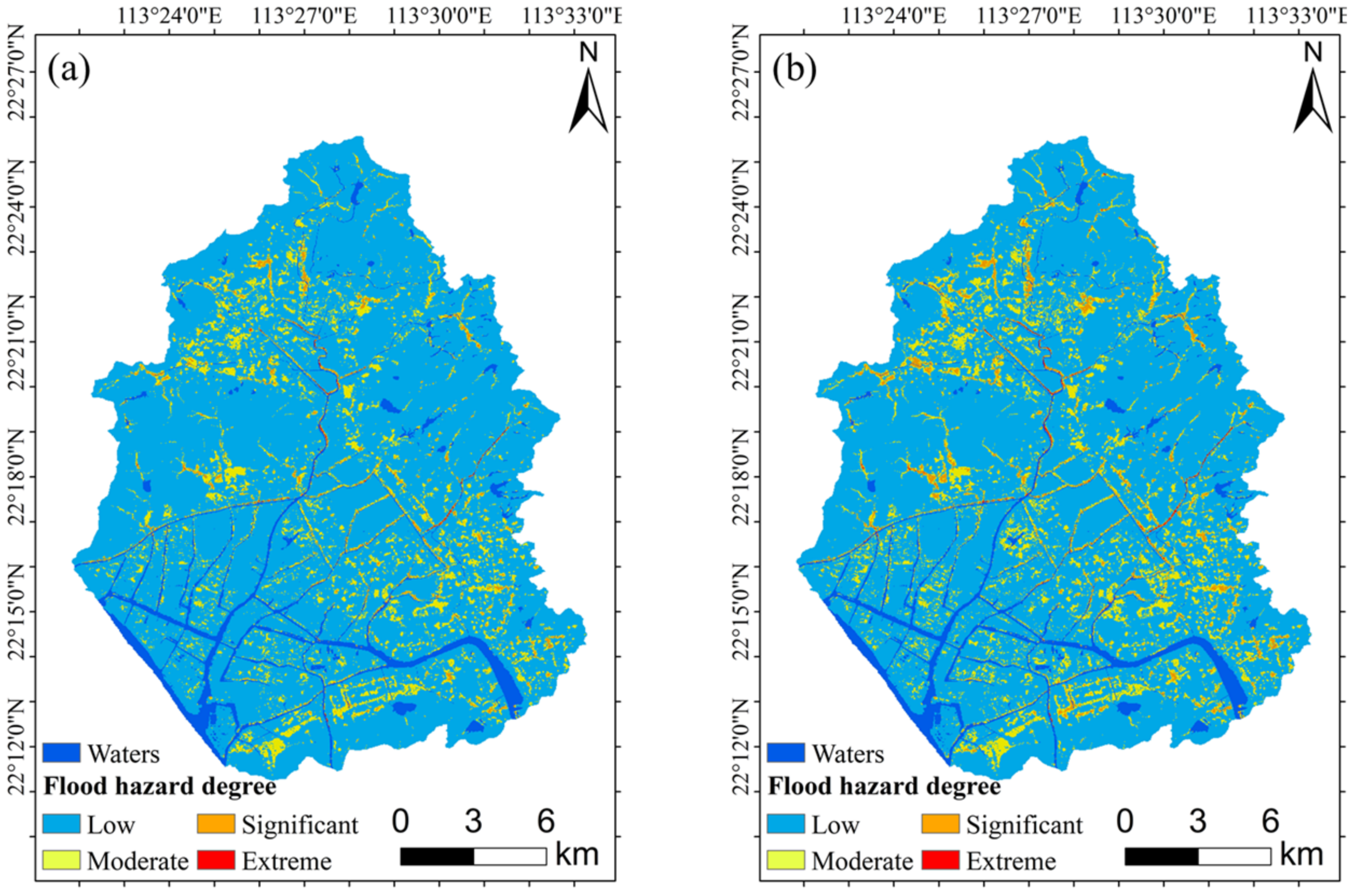
3.2. Flood Hazard Classification Results
3.3. Flood Disaster Loss Dynamic Assessment
3.3.1. Spatialization of Fine-Resolution GDP and Population Data Based on POIs Kernel Density
3.3.2. Dynamic Assessment of the Effect of Flood Disaster on GDP
3.3.3. Dynamic Assessment of the Effect of Flood Disaster on Population
4. Discussion
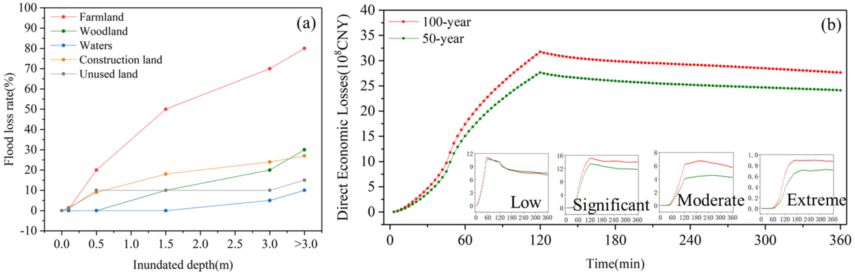
4.1. The Development Rules of Flood Disaster Loss under Different Flood Hazards
4.2. Suggestions on Measures to Reduce Flood Disaster Loss
4.3. Uncertainty in Research
4.3.1. The Uncertainty of Flood Simulation
4.3.2. The Uncertainty of Flood Disaster Loss Assessment
4.3.3. The Uncertainty of Machine Learning
4.4. Future Studies
- The prediction accuracy of the GDP spatial distribution data was 65%. Future studies should try some methods to solve this problem, such as adding training samples, increasing the type of input variables, or comparing the accuracy of different machine learning methods;
- Machine learning algorithms have been widely used, but they are rarely used in the field of urban hydrology. This study attempted to use machine learning algorithms to obtain fine-resolution socio-economic data, which provided data for a flood disaster loss assessment. Future studies should explore the application of machine learning algorithms in the field of urban hydrology such as obtaining flood inundation maps based on machine learning to improve the timeliness of flood simulations;
- The results of this study showed that the return period had an effect on the initial time and peak occurrence time of the flood disaster. However, only two rainstorm situations were set in this study, resulting in limitations in the conclusions. Future studies will construct a variety of rainstorm situations by setting different peak coefficients, rainfall durations, and return periods to investigate the dynamic assessment of flood disaster loss under various rainstorm designs, and to identify the influence of rainfall characteristics on the development process of flood disaster loss;
- Different from property distribution, people should adopt different risk avoidance strategies, which would lead to a great uncertainty when using a static assessment method to calculate the number of the affected population. Therefore, future research should combine the multi-agent model to study the impact of different risk avoidance strategies on the number of the affected population and improve the accuracy of the assessment model.
5. Conclusions
- Under extreme rainstorm conditions, flood disaster had a serious impact on economy and population. For the 50- and 100-year return periods, the maximum direct economic loss was 2.77 billion CNY and 3.18 billion CNY, respectively, accounting for 2.63% and 3.02% of the total GDP, respectively. The affected population was 160,303 and 189,924, respectively, accounting for 14.76% and 17.49% of the total population, respectively;
- The higher degree flood hazard areas were mainly distributed on built-up land. Moreover, with the increase in the return period, the higher degree flood hazard areas had a greater proportion of increase;
- In terms of the occurrence time of flood disaster loss, the initial time and the peak time of flood disaster loss increased with an increasing flood hazard degree and decreased with the increase in the return period. In terms of the flood disaster loss, in moderate-, significant-, and extreme-degree hazard areas, the total loss increased with the increase in the return period, and the unit loss decreased with the increase in the return period;
- Under the design rainstorm scenario of the Chicago rain pattern, the process of flood loss development had a stage of rapid increase.
Author Contributions
Funding
Institutional Review Board Statement
Informed Consent Statement
Data Availability Statement
Acknowledgments
Conflicts of Interest
References
- Wu, Z.; Shen, Y.; Wang, H.; Wu, M. Urban flood disaster risk evaluation based on ontology and Bayesian Network. J. Hydrol. 2020, 583, 124596. [Google Scholar] [CrossRef]
- Luo, P.; Mu, D.; Xue, H.; Ngo-Duc, T.; Dang-Dinh, K.; Takara, K.; Nover, D.; Schladow, G. Flood inundation assessment for the Hanoi Central Area, Vietnam under historical and extreme rainfall conditions. Sci. Rep. 2018, 8, 12623. [Google Scholar] [CrossRef]
- Mu, D.; Luo, P.; Lyu, J.; Zhou, M.; Huo, A.; Duan, W.; Nover, D.; He, B.; Zhao, X. Impact of temporal rainfall patterns on flash floods in Hue City, Vietnam. J. Flood Risk Manag. 2020, 14, e12668. [Google Scholar] [CrossRef]
- Chao, L.; Zhang, K.; Li, Z.; Wang, J.; Yao, C.; Li, Q. Applicability assessment of the CASCade Two Dimensional SEDiment (CASC2D-SED) distributed hydrological model for flood forecasting across four typical medium and small watersheds in China. J. Flood Risk Manag. 2019, 12, e12518. [Google Scholar] [CrossRef] [Green Version]
- Cai, T.; Li, X.; Ding, X.; Wang, J.; Zhan, J. Flood risk assessment based on hydrodynamic model and fuzzy comprehensive evaluation with GIS technique. Int. J. Disaster Risk Reduct. 2019, 35, 101077. [Google Scholar] [CrossRef]
- Scawthorn, C.; Blais, N.; Seligson, H.; Tate, E.; Mifflin, E.; Thomas, W.; Murphy, J.; Jones, C. HAZUS-MH flood loss estimation methodology. I: Overview and flood hazard characterization. Nat. Hazards Rev. 2006, 7, 60–71. [Google Scholar] [CrossRef]
- Scawthorn, C.; Flores, P.; Blais, N.; Seligson, H.; Tate, E.; Chang, S.; Mifflin, E.; Thomas, W.; Murphy, J.; Jones, C. HAZUS-MH flood loss estimation methodology. II. Damage and loss assessment. Nat. Hazards Rev. 2006, 7, 72–81. [Google Scholar] [CrossRef]
- Thieken, A.; Olschewski, A.; Kreibich, H.; Kobsch, S.; Merz, B. Development and evaluation of FLEMOps–a new Flood Loss Estimation MOdel for the private sector. WIT Trans. Ecol. Environ. 2008, 118, 315–324. [Google Scholar] [CrossRef]
- Meyer, V.; Scheuer, S.; Haase, D. A multicriteria approach for flood risk mapping exemplified at the Mulde river, Germany. Nat. Hazards 2009, 48, 17–39. [Google Scholar] [CrossRef]
- Aznar-Siguan, G.; Bresch, D.N. CLIMADA v1: A global weather and climate risk assessment platform. Geosci. Model Dev. 2019, 12, 3085–3097. [Google Scholar] [CrossRef] [Green Version]
- Amadio, M.; Mysiak, J.; Carrera, L.; Koks, E. Improving flood damage assessment models in Italy. Nat. Hazards 2016, 82, 2075–2088. [Google Scholar] [CrossRef] [Green Version]
- Husby, T.G.; de Groot, H.L.; Hofkes, M.W.; Dröes, M.I. Do floods have permanent effects? Evidence from the Netherlands. J. Reg. Sci. 2014, 54, 355–377. [Google Scholar] [CrossRef]
- Guha-Sapir, D.; Rodriguez-Llanes, J.M.; Jakubicka, T. Using disaster footprints, population databases and GIS to overcome persistent problems for human impact assessment in flood events. Nat. Hazards 2011, 58, 845–852. [Google Scholar] [CrossRef] [Green Version]
- Feng, Q.; Liu, J.; Gong, J. Urban flood mapping based on unmanned aerial vehicle remote sensing and random forest classifier—A case of Yuyao, China. Water 2015, 7, 1437–1455. [Google Scholar] [CrossRef]
- Smith, A.; Bates, P.D.; Wing, O.; Sampson, C.; Quinn, N.; Neal, J. New estimates of flood exposure in developing countries using high-resolution population data. Nat. Commun. 2019, 10, 1–7. [Google Scholar] [CrossRef] [PubMed] [Green Version]
- Mosavi, A.; Ozturk, P.; Chau, K.-w. Flood prediction using machine learning models: Literature review. Water 2018, 10, 1536. [Google Scholar] [CrossRef] [Green Version]
- Zhang, S.; Zhang, W.; Wang, Y.; Zhao, X.; Song, P.; Tian, G.; Mayer, A.L. Comparing human activity density and green space supply using the Baidu Heat Map in Zhengzhou, China. Sustainability 2020, 12, 7075. [Google Scholar] [CrossRef]
- Weiwei, S.; Xin, S.; Jie, L.; Jiahong, L.; Zhiyong, Y.; Yongqiang, C.; Zhaohui, Y.; Kaibo, W. The application of big data in the analysis of the impact of urban floods: A case study of Qianshan River Basin. J. Phys. Conf. Ser. 2021, 1955, 012061. [Google Scholar] [CrossRef]
- Merz, B.; Kreibich, H.; Schwarze, R.; Thieken, A. Review article ”Assessment of economic flood damage”. Nat. Hazard Earth Sys. 2010, 10, 1697–1724. [Google Scholar] [CrossRef]
- Huang, W. Macro Analysis of Urban Structure Based on Point of Interest. In Proceedings of the 2016 6th International Conference on Mechatronics, Computer and Education Informationization (MCEI 2016), Shenyang, China, 11–13 November 2016; pp. 928–932. [Google Scholar]
- Li, K.; Chen, Y.; Li, Y. The random forest-based method of fine-resolution population spatialization by using the international space station nighttime photography and social sensing data. Remote Sens. 2018, 10, 1650. [Google Scholar] [CrossRef] [Green Version]
- Wang, Y.; Huang, C.; Zhao, M.; Hou, J.; Zhang, Y.; Gu, J. Mapping the Population Density in Mainland China Using NPP/VIIRS and Points-Of-Interest Data Based on a Random Forests Model. Remote Sens. 2020, 12, 3645. [Google Scholar] [CrossRef]
- Zhang, A.; Pan, Y.; Ming, Y.; Wang, J. Research of GDP Spatialization based on Multi-source Information Coupling: A Case Study in Beijing. Remote Sens. Technol. Appl. 2021, 36, 463–472. [Google Scholar] [CrossRef]
- Apel, H.; Aronica, G.; Kreibich, H.; Thieken, A. Flood risk analyses—how detailed do we need to be? Nat. Hazards 2009, 49, 79–98. [Google Scholar] [CrossRef]
- Zhou, Q.; Mikkelsen, P.S.; Halsnæs, K.; Arnbjerg-Nielsen, K. Framework for economic pluvial flood risk assessment considering climate change effects and adaptation benefits. J. Hydrol. 2012, 414, 539–549. [Google Scholar] [CrossRef]
- Mei, C.; Liu, J.; Wang, H.; Yang, Z.; Ding, X.; Shao, W. Integrated assessments of green infrastructure for flood mitigation to support robust decision-making for sponge city construction in an urbanized watershed. Sci. Total Environ. 2018, 639, 1394–1407. [Google Scholar] [CrossRef]
- Bisht, D.S.; Chatterjee, C.; Kalakoti, S.; Upadhyay, P.; Sahoo, M.; Panda, A. Modeling urban floods and drainage using SWMM and MIKE URBAN: A case study. Nat. Hazards 2016, 84, 749–776. [Google Scholar] [CrossRef]
- Sheng, J.G.; Dan, Y.D.; Liu, C.S.; Ma, L.M. Study of Simulation in Storm Sewer System of Zhenjiang Urban by Infoworks ICM Model. In Applied Mechanics and Materials; Trans Tech Publications Ltd.: Bäch, Switzerland, 2012; pp. 683–686. [Google Scholar]
- Mei, C.; Liu, J.; Wang, H.; Li, Z.; Yang, Z.; Shao, W.; Ding, X.; Weng, B.; Yu, Y.; Yan, D. Urban flood inundation and damage assessment based on numerical simulations of design rainstorms with different characteristics. Sci. China Technol. Sci. 2020, 63, 2292–2304. [Google Scholar] [CrossRef]
- Jahanbazi, M.; Egger, U. Application and comparison of two different dual drainage models to assess urban flooding. Urban Water J. 2014, 11, 584–595. [Google Scholar] [CrossRef]
- Li, Z.; Liu, J.; Mei, C.; Shao, W.; Wang, H.; Yan, D. Comparative Analysis of Building Representations in TELEMAC-2D for Flood Inundation in Idealized Urban Districts. Water 2019, 11, 1840. [Google Scholar] [CrossRef] [Green Version]
- Zhu, J.; Dai, Q.; Deng, Y.; Zhang, A.; Zhang, Y.; Zhang, S. Indirect damage of urban flooding: Investigation of flood-induced traffic congestion using dynamic modeling. Water 2018, 10, 622. [Google Scholar] [CrossRef] [Green Version]
- He, J.; Qiang, Y.; Luo, H.; Zhou, S.; Zhang, L. A stress test of urban system flooding upon extreme rainstorms in Hong Kong. J. Hydrol. 2021, 597, 125713. [Google Scholar] [CrossRef]
- Romali, N.S.; Yusop, Z.; Ismail, Z. Flood damage assessment: A review of flood stage–damage function curve. In ISFRAM 2014; Springer: Singapore, 2015; pp. 147–159. [Google Scholar] [CrossRef] [Green Version]
- Romali, N.S.; Yusop, Z. Flood damage and risk assessment for urban area in Malaysia. Hydrol. Res. 2021, 52, 142–159. [Google Scholar] [CrossRef]
- Li, W.; Guo, X.; Mao, X.; Xiao, D.; Lai, W.; Wang, H. The dynamic population risk assessment model for rainstorm-flood utilization multi-agent. J. Catastrophol. 2015, 30, 80–87. [Google Scholar]
- Pyatkova, K.; Chen, A.S.; Butler, D.; Vojinović, Z.; Djordjević, S. Assessing the knock-on effects of flooding on road transportation. J. Environ. Manag. 2019, 244, 48–60. [Google Scholar] [CrossRef] [PubMed]
- Yang, X.; Chen, H.; Wang, Y.; Xu, C.-Y. Evaluation of the effect of land use/cover change on flood characteristics using an integrated approach coupling land and flood analysis. Hydrol. Res. 2016, 47, 1161–1171. [Google Scholar] [CrossRef] [Green Version]
- Bai, Z.; Wang, J.; Wang, M.; Gao, M.; Sun, J. Accuracy assessment of multi-source gridded population distribution datasets in China. Sustainability 2018, 10, 1363. [Google Scholar] [CrossRef] [Green Version]
- Mei, C. Development of a Coupled Urban Hydrological-Hydrodynamic Model and Its Application; China Institute of Water Resources and Hydropower Resources: Beijing, China, 2019. [Google Scholar]
- Chen, W.J. Urban Flood Hydrological and Hydrodynamic Model Construction and Flood Management Key Issues Exploration; South China University of Technology: Guangzhou, China, 2019. [Google Scholar]
- Kvočka, D.; Falconer, R.A.; Bray, M. Flood hazard assessment for extreme flood events. Nat. Hazards 2016, 84, 1569–1599. [Google Scholar] [CrossRef] [Green Version]
- Defra, U. Defra Flood and Coastal Defence Appraisal Guidance, Social Appraisal, Supplementary Note to Operating Authorities: Assessing and Valuing the Risk to Life from Flooding for Use in Appraisal of Risk Management Measures. 2008. Available online: https://assets.publishing.service.gov.uk/government/uploads/system/uploads/attachment_data/file/181441/risktopeople.pdf (accessed on 30 September 2021).
- Wade, S.; Ramsbottom, D.; Floyd, P.; Penning-Rowsell, E.; Surendran, S. Risks to People: Developing New Approaches for Flood Hazard and Vulnerability Mapping. 2005. Available online: http://eprints.hrwallingford.com/id/eprint/562/ (accessed on 26 September 2021).
- Coulibaly, G.; Leye, B.; Tazen, F.; Mounirou, L.A.; Karambiri, H. Urban Flood Modeling Using 2D Shallow-Water Equations in Ouagadougou, Burkina Faso. Water 2020, 12, 2120. [Google Scholar] [CrossRef]
- Lyu, H.; Ni, G.; Cao, X.; Ma, Y.; Tian, F. Effect of temporal resolution of rainfall on simulation of urban flood processes. Water 2018, 10, 880. [Google Scholar] [CrossRef] [Green Version]
- Jang, J.-H.; Chang, T.-H.; Chen, W.-B. Effect of inlet modelling on surface drainage in coupled urban flood simulation. J. Hydrol. 2018, 562, 168–180. [Google Scholar] [CrossRef]
- Shi, R.; Liu, N.; Li, L.; Ye, L.; Liu, X.; Guo, G. Application of rainstorm and flood inundation model in flood disaster economic loss evaluation. Torrential Rain Disasters 2013, 32, 379–384. [Google Scholar]
- Lu, Z. Evaluation and Analysis of Flood Disaster Loss in the Pearl River Delta. Guangdong Water Resour. Hydropower 2010, 3, 17–21. [Google Scholar] [CrossRef]
- Shao, W.; Su, X.; Lu, J.; Liu, J.; Yang, Z.; Mei, C.; Liu, C.; Lu, J. Urban Resilience of Shenzhen City under Climate Change. Atmosphere 2021, 12, 537. [Google Scholar] [CrossRef]
- Jia, H.; Wang, Z.; Zhen, X.; Clar, M.; Shaw, L.Y. China’s sponge city construction: A discussion on technical approaches. Front. Environ. Sci. Eng. 2017, 11, 1–11. [Google Scholar] [CrossRef]
- Yuanyuan, W.; Ping, L.; Wenze, S.; Xinchun, Y. A new framework on regional smart water. Procedia Comput. Sci. 2017, 107, 122–128. [Google Scholar] [CrossRef]
- Lee, J.H.; Hancock, M.G.; Hu, M.-C. Towards an effective framework for building smart cities: Lessons from Seoul and San Francisco. Technol. Forecast. Soc. Change 2014, 89, 80–99. [Google Scholar] [CrossRef]
- Surminski, S. The role of insurance in reducing direct risk: The case of flood insurance. Int. Rev. Environ. Resour. Econ. 2014, 7, 241–278. [Google Scholar] [CrossRef] [Green Version]
- Liu, Y.; Li, H.; Yang, C.; Zhang, B.; He, M.; Chang, Q. Spatialization of GDP Based on Remote Sensing Data and POI Data: A Case Study of Beijing City. Areal Res. Dev. 2021, 40, 27–39. [Google Scholar]
- Wang, L.; Fan, H.; Wang, Y. Fine-resolution population mapping from international space station nighttime photography and multisource social sensing data based on similarity matching. Remote Sens. 2019, 11, 1900. [Google Scholar] [CrossRef] [Green Version]
- Wang, L.; Fan, H.; Wang, Y. Improving population mapping using Luojia 1-01 nighttime light image and location-based social media data. Sci. Total Environ. 2020, 730, 139148. [Google Scholar] [CrossRef]
- Akossou, A.; Palm, R. Impact of Data Structure on the Estimators R-square and Adjusted R-square in Linear Regression. Int. J. Math. Comput 2013, 20, 84–93. [Google Scholar]


| CN Value | Class A Soil | Class B Soil | Class C Soil | Class D Soil |
|---|---|---|---|---|
| Waters | 98 | 98 | 98 | 98 |
| Woodland | 30 | 55 | 70 | 77 |
| Farmland | 49 | 69 | 79 | 84 |
| Built-up land | 89 | 92 | 94 | 95 |
| Unused land | 81 | 88 | 91 | 93 |
| Type of Land Use | Waters | Woodland | Farmland | Built-Up Land | Unused Land |
|---|---|---|---|---|---|
| Manning coefficient | 0.027 | 0.15 | 0.035 | 0.016 | 0.025 |
| Depth (cm) | Number of WPs | The Average Inundation Depth (cm) | ||
|---|---|---|---|---|
| 50-Year | 100-Year | 50-Year | 100-Year | |
| <15 | 22 | 20 | 4 | 3 |
| 15–30 | 25 | 24 | 22 | 23 |
| >30 | 34 | 37 | 67 | 70 |
| Land Use Types | Return Period | Flood Hazard Degrees | |||
|---|---|---|---|---|---|
| Low | Moderate | Significant | Extreme | ||
| Woodland | 50-year | 95.39 | 2.50 | 0.50 | 0.02 |
| 100-year | 94.04 | 3.45 | 0.86 | 0.06 | |
| Farmland | 50-year | 65.86 | 1.55 | 0.35 | 0.05 |
| 100-year | 64.94 | 2.22 | 0.57 | 0.09 | |
| Built-up land | 50-year | 119.92 | 25.04 | 3.83 | 0.23 |
| 100-year | 113.64 | 28.86 | 6.13 | 0.38 | |
| Algorithm | Hyperparameters | R-Square | Hyperparameters | R-Square | ||
|---|---|---|---|---|---|---|
| GDP | Population | |||||
| Train Set | Test Set | Train Set | TEST SET | |||
| Random Forest | bootstrap: ‘True’ max_depth: 30 max_features: ‘log2′ min_samples_leaf: 1 min_samples_split: 2 n_estimators: 260 | 0.9244 | 0.6549 | bootstrap: ‘True’ max_depth: 80 max_features: ‘auto’ min_samples_leaf: 1 min_samples_split: 2 n_estimators: 340 | 0.9742 | 0.8368 |
| Disaster-Bearing Bodies | Return Period | The Initial Time of Flood Disaster Loss (thmin) | Trend | |||
|---|---|---|---|---|---|---|
| Low | Moderate | Significant | Extreme | |||
| GDP | 50-year | 3 | 18 | 30 | 45 | ↑ |
| 100-year | 3 | 15 | 24 | 39 | ↑ | |
| Trend | --- | ↓ | ↓ | ↓ | ||
| Population | 50-year | --- | 18 | 30 | 45 | ↑ |
| 100-year | --- | 18 | 27 | 42 | ↑ | |
| Trend | --- | ↓ | ↓ | ↓ | ||
| Disaster-Bearing Bodies | Return Period | The Peak Time of Flood Disaster Loss (thmin) | Trend | |||
|---|---|---|---|---|---|---|
| Low | Moderate | Significant | Extreme | |||
| GDP | 50-year | 63 | 123 | 264 | 330 | ↑ |
| 100-year | 57 | 120 | 192 | 246 | ↑ | |
| Trend | ↓ | ↓ | ↓ | ↓ | ||
| Population | 50-year | --- | 120 | 129 | 345 | ↑ |
| 100-year | --- | 120 | 126 | 324 | ↑ | |
| Trend | --- | --- | ↓ | ↓ | ||
| Disaster-Bearing Bodies | Return Period | Statistical Objects | Flood Loss under Different Flood Hazard Degrees | |||
|---|---|---|---|---|---|---|
| Low | Moderate | Significant | Extreme | |||
| GDP | 50-year | Total | 106,667.12 | 133,422.35 | 45,500.95 | 7301.00 |
| Unit area | 347.79 | 4583.16 | 8544.30 | 12,577.09 | ||
| 100-year | Total | 110,196.26 | 151,310.90 | 67,224.17 | 9032.20 | |
| Unit area | 356.42 | 4382.20 | 7962.21 | 12,451.33 | ||
| Population | 50-year | Total | --- | 136,231 | 23,075 | 2197 |
| Unit area | --- | 4683 | 4694 | 3791 | ||
| 100-year | Total | --- | 152,211 | 36,242 | 2785 | |
| Unit area | --- | 4408 | 4503 | 3692 | ||
Publisher’s Note: MDPI stays neutral with regard to jurisdictional claims in published maps and institutional affiliations. |
© 2021 by the authors. Licensee MDPI, Basel, Switzerland. This article is an open access article distributed under the terms and conditions of the Creative Commons Attribution (CC BY) license (https://creativecommons.org/licenses/by/4.0/).
Share and Cite
Su, X.; Shao, W.; Liu, J.; Jiang, Y.; Wang, K. Dynamic Assessment of the Impact of Flood Disaster on Economy and Population under Extreme Rainstorm Events. Remote Sens. 2021, 13, 3924. https://doi.org/10.3390/rs13193924
Su X, Shao W, Liu J, Jiang Y, Wang K. Dynamic Assessment of the Impact of Flood Disaster on Economy and Population under Extreme Rainstorm Events. Remote Sensing. 2021; 13(19):3924. https://doi.org/10.3390/rs13193924
Chicago/Turabian StyleSu, Xin, Weiwei Shao, Jiahong Liu, Yunzhong Jiang, and Kaibo Wang. 2021. "Dynamic Assessment of the Impact of Flood Disaster on Economy and Population under Extreme Rainstorm Events" Remote Sensing 13, no. 19: 3924. https://doi.org/10.3390/rs13193924
APA StyleSu, X., Shao, W., Liu, J., Jiang, Y., & Wang, K. (2021). Dynamic Assessment of the Impact of Flood Disaster on Economy and Population under Extreme Rainstorm Events. Remote Sensing, 13(19), 3924. https://doi.org/10.3390/rs13193924