
Estimation of Apple Tree Leaf Chlorophyll Content Based on Machine Learning Methods


Abstract
:1. Introduction
2. Materials and Methods
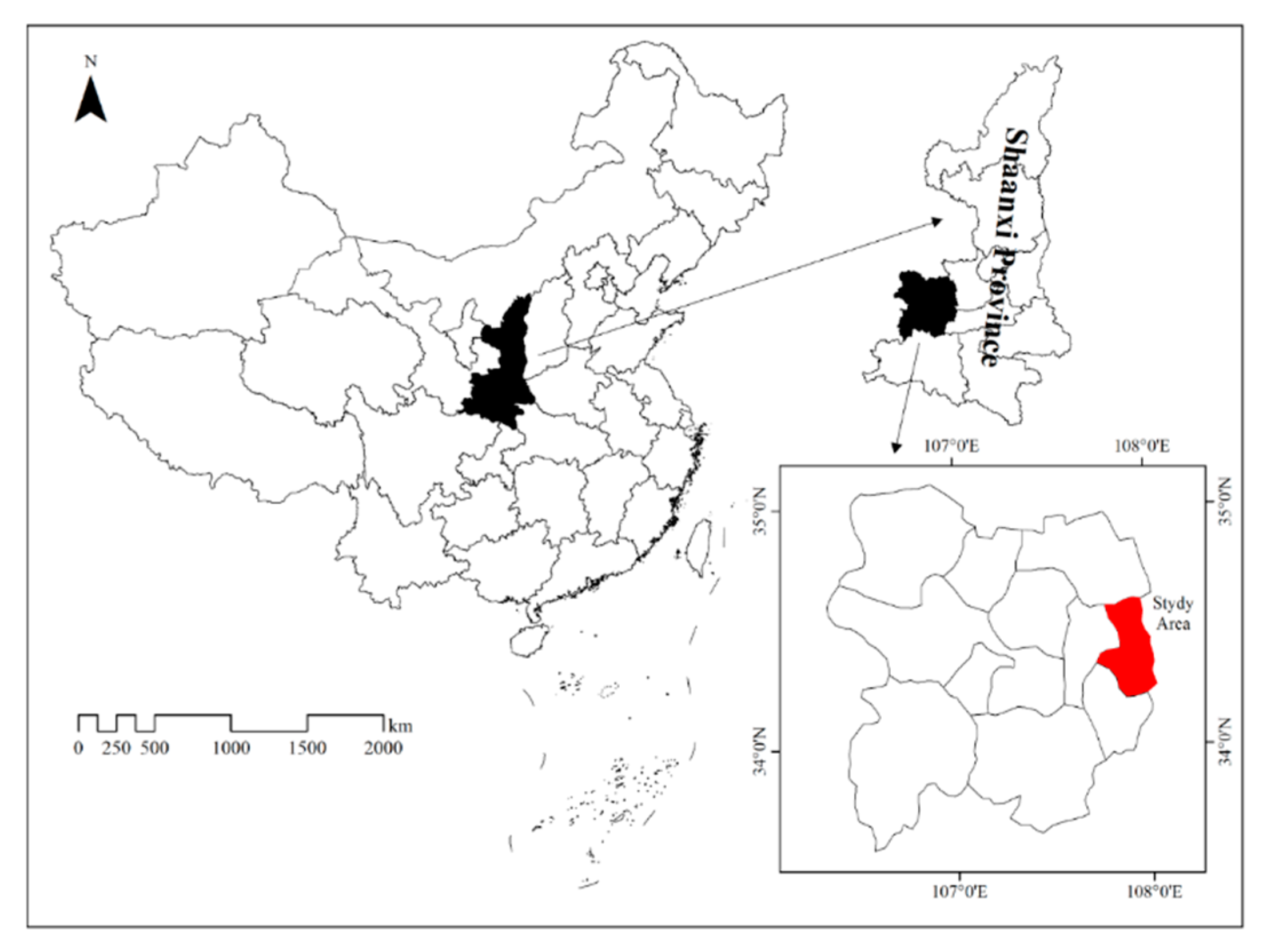
2.1. Study Area and Experimental Setup
2.2. Hyperspectral Data Acquisition
2.3. Leaf Chlorophyll Content Measurement
2.4. Methods
2.4.1. Spectral Transformation (ST)
2.4.2. Vegetation Indices
2.4.3. Three Edge Parameters

| Parameters | Explanation | References |
|---|---|---|
| ST (1) | ||
| OS | Original spectrum | [19] |
| RS | Reciprocal transformed spectrum | [19] |
| FODS | First-order differential spectrum | [19] |
| CRS | Continuum removal spectrum | [19] |
| VIs (2) | ||
| Normalized difference Vegetation index (NDVI) | (R800 − R670)/(R800 + R670) | [24] |
| Ratio vegetation index (RVI) | R765/R720 | [27] |
| Green ratio vegetation index (GRVI) | (R620 − R506)/(R620 + R506) | [29] |
| Photochemical reflectance Index (PRI) | (R570 − R531)/(R570 + R531) | [30] |
| Normalized pigment chlorophyll index (NPCI) | (R642 − R432)/(R642 + R432) | [31] |
| Modified red edge simple ratio index (mSR705) | (R750 − R445)/(R705 − R445) | [25] |
| Plant pigment ratio (PPR) | (R503 − R436)/(R503 + R436) | [32] |
| Structure intensive pigment index (SIPI) | (R800 − R445)/(R800 − R680) | [33] |
| Normalized difference spectral index (NDSI) | (R813 − R763)/(R813 + R763) | [34] |
| Leaf chlorophyll index (LCI) | (R850 − R710)/(R850 − R680) | [26] |
| TEP (3) | ||
| Db | First-order differential spectrum maximum in the wavelength range of 490~530 nm | [35] |
| Dy | First-order differential spectrum maximum in the wavelength range of 560~640 nm | [35] |
| Dr | First-order differential spectrum maximum in the wavelength range of 680~760 nm | [35] |
| SDb | First-order differential spectral integration in the wavelength range of 490~530 nm | [35] |
| SDy | First-order differential spectral integration in the wavelength range 560~640 nm | [35] |
| SDr | First-order differential spectral integration in the wavelength range of 680~760 nm | [35] |
| SDr/SDb | Ratio of the red edge area to the blue edge area | [35] |
| SDr/SDy | Ratio of the red edge area to the yellow edge area | [35] |
| (SDr − SDb)/(SDr + SDb) | Normalized value of the red edge area and the blue edge area | [35] |
| (SDr − SDy)/(SDr + SDy) | Normalized value of the red edge area and the yellow edge area | [35] |
2.4.4. Linear Regression Analysis
2.4.5. Random Forest (RF) Regression
2.4.6. Support Vector Regression (SVR)
2.5. Data Analysis
2.6. Calibration and Validation
3. Results
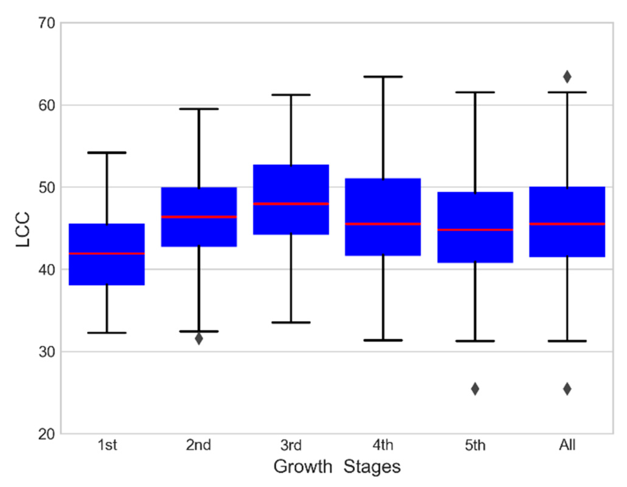
3.1. Descriptive Analysis of Measured LCC
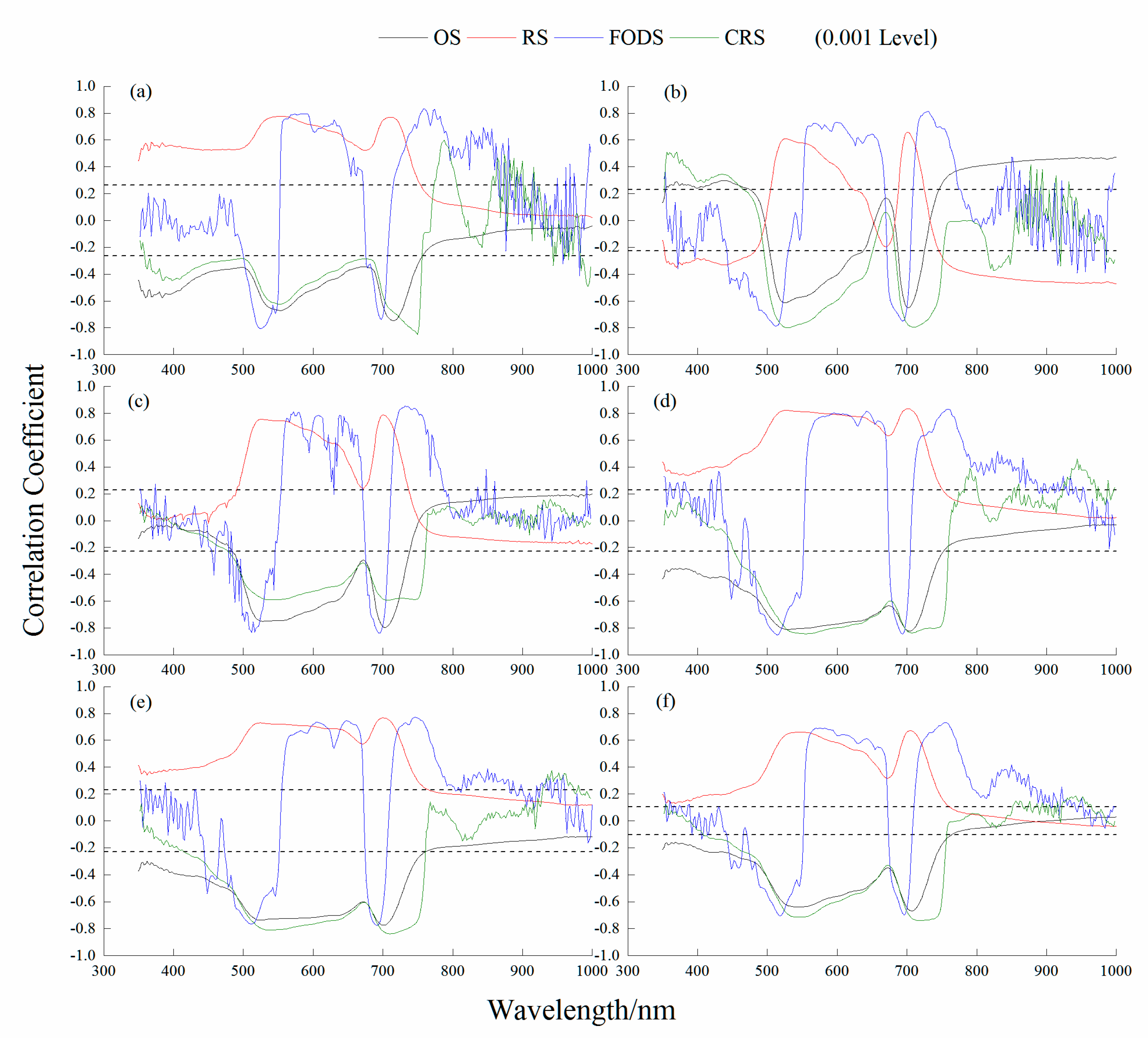
3.2. Selection of Sensitivity Parameters
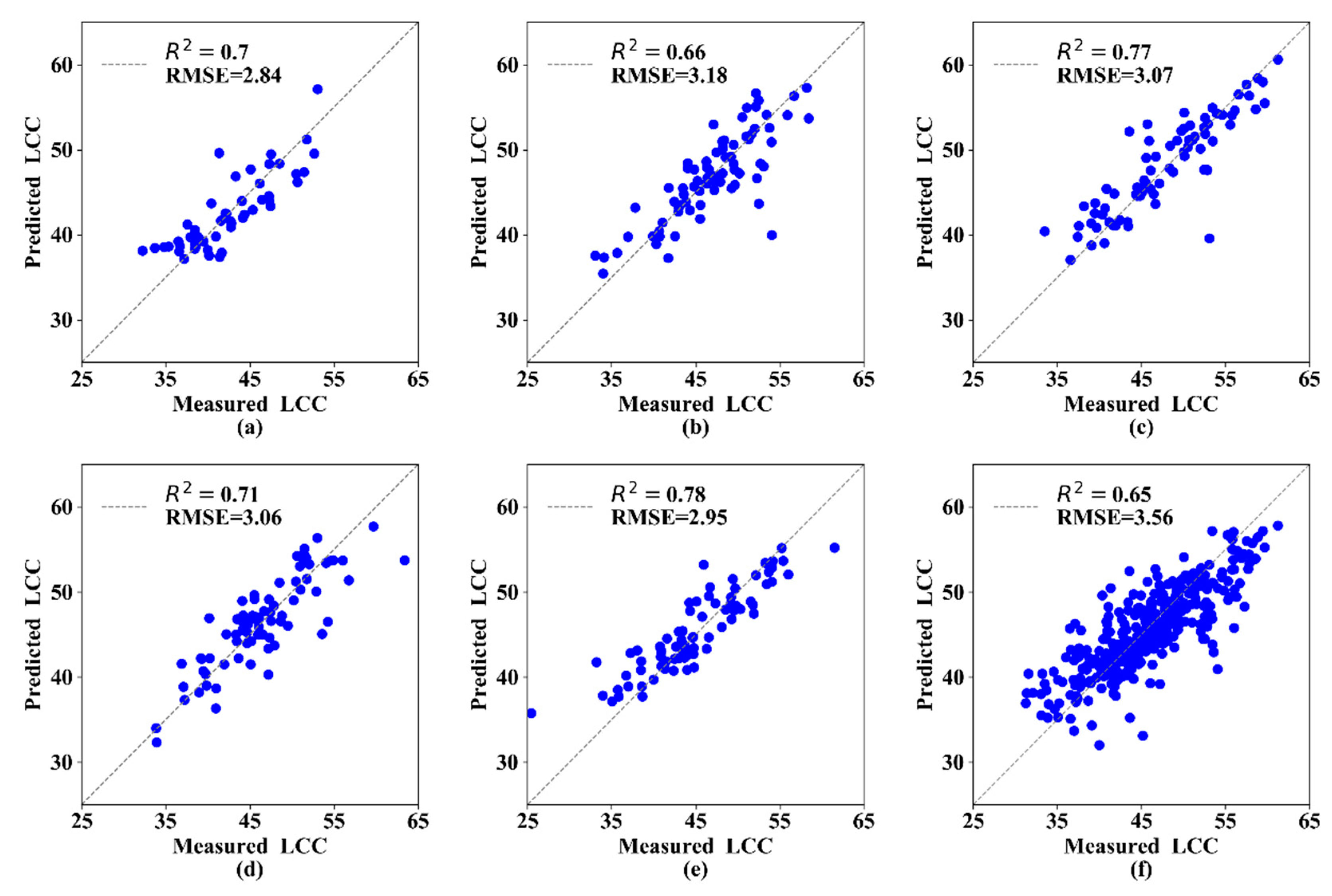
3.3. ULR
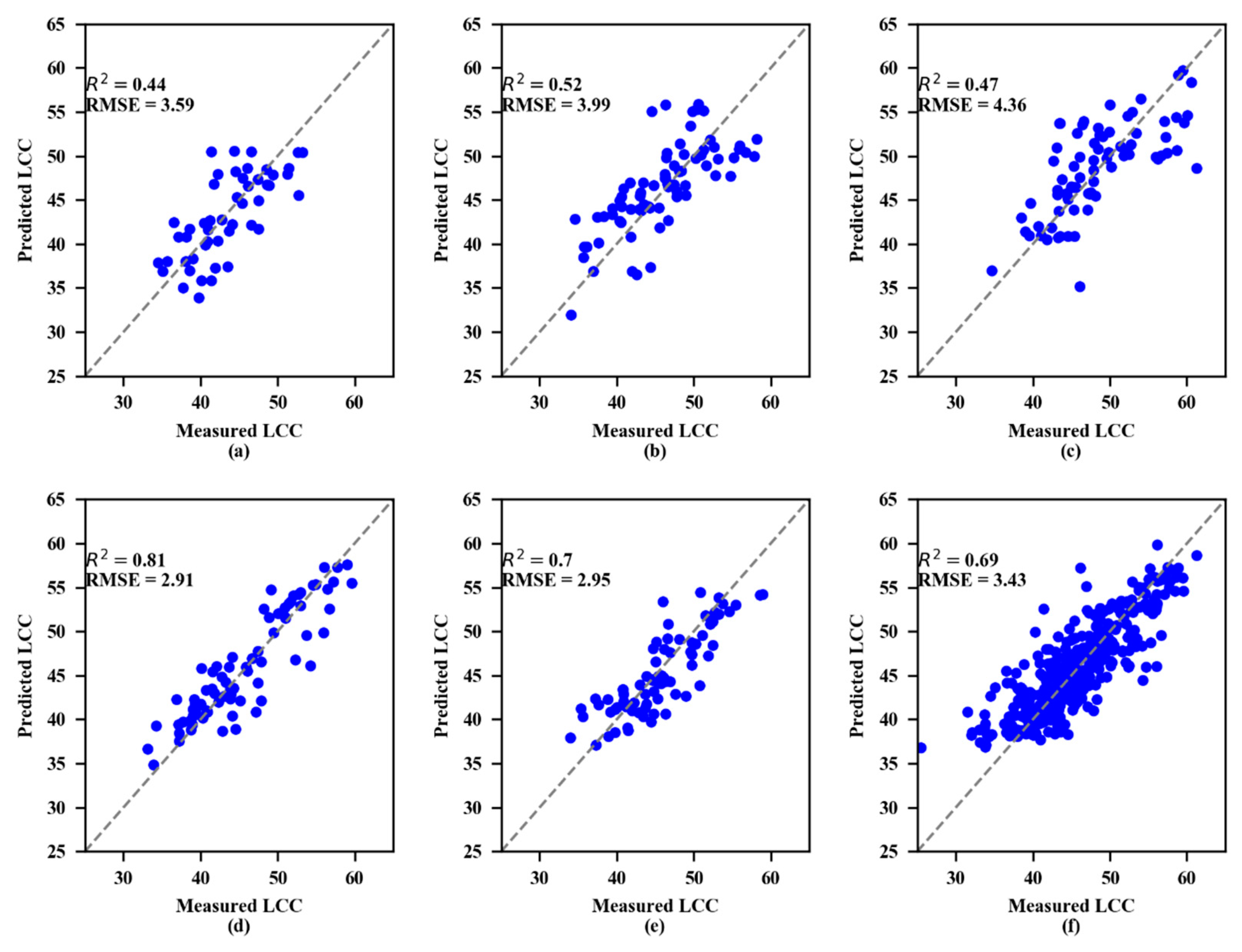
3.4. MLR
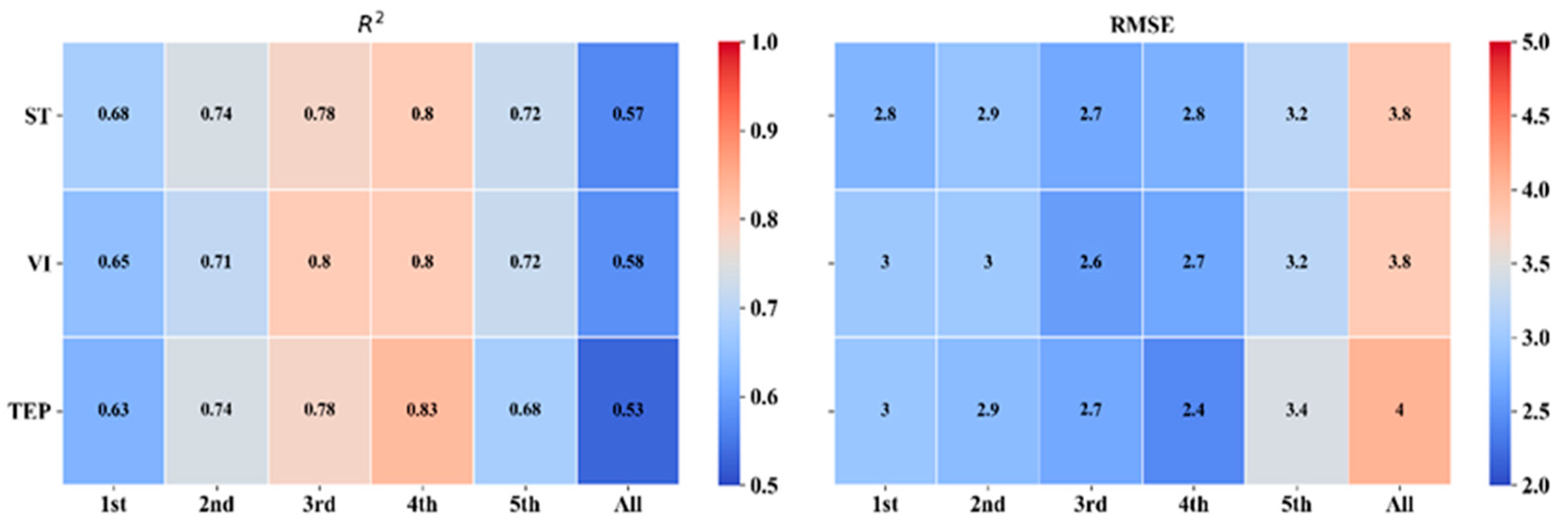
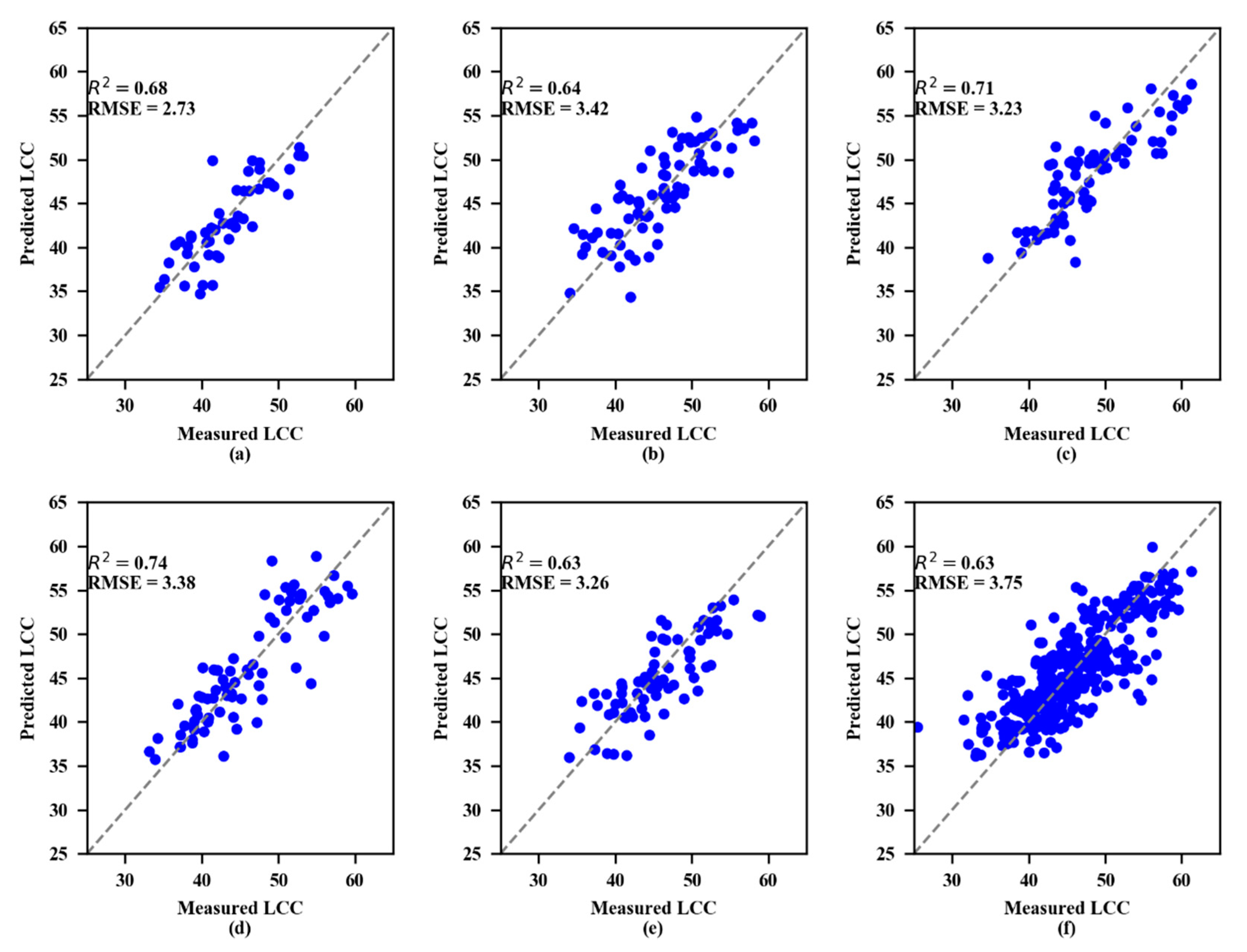
3.5. Machine Learning Models
4. Discussion
4.1. Selected Optimized Spectral Indices
4.2. Comparison of Estimation Models with LCC
4.3. Challenges and Future Research
5. Conclusions
Author Contributions
Funding
Informed Consent Statement
Data Availability Statement
Conflicts of Interest
References
- Gitelson, A.A.; Merzlyak, M.N. Remote estimation of chlorophyll content in higher plant leaves. Int. J. Remote Sens. 1997, 18, 2691–2697. [Google Scholar] [CrossRef]
- Peng, Y.; Nguy-Robertson, A.; Arkebauer, T.; Gitelson, A.A. Assessment of Canopy Chlorophyll Content Retrieval in Maize and Soybean: Implications of Hysteresis on the Development of Generic Algorithms. Remote Sens. 2017, 9, 226. [Google Scholar] [CrossRef] [Green Version]
- Merzlyak, M.N.; Gitelson, A.A.; Chivkunova, O.B.; Rakitin, V.Y. Non-destructive optical detection of pigment changes during leaf senescence and fruit ripening. Physiol. Plant. 1999, 106, 135–141. [Google Scholar] [CrossRef] [Green Version]
- Ustin, S.L.; Valko, P.G.; Kefauver, S.C.; Santos, M.J.; Zimpfer, J.F.; Smith, S.D. Remote sensing of biological soil crust under simulated climate change manipulations in the Mojave Desert. Remote Sens. Environ. 2009, 113, 317–328. [Google Scholar] [CrossRef]
- Gitelson, A.A.; Viña, A.; Ciganda, V.; Rundquist, D.C.; Arkebauer, T.J. Remote estimation of canopy chlorophyll content in crops. Geophys. Res. Lett. 2005, 32, 1–4. [Google Scholar] [CrossRef] [Green Version]
- Upreti, D.; Huang, W.; Kong, W.; Pascucci, S.; Pignatti, S.; Zhou, X.; Ye, H.; Casa, R. A Comparison of Hybrid Machine Learning Algorithms for the Retrieval of Wheat Biophysical Variables from Sentinel-2. Remote Sens. 2019, 11, 481. [Google Scholar] [CrossRef] [Green Version]
- Peuelas, J.; Filella, I. Visible and near-infrared reflectance techniques for diagnosing plant physiological status. Trends Plant Sci. 1998, 3, 151–156. [Google Scholar] [CrossRef]
- Shah, S.H.; Angel, Y.; Houborg, R.; Ali, S.; McCabe, M.F. A Random Forest Machine Learning Approach for the Retrieval of Leaf Chlorophyll Content in Wheat. Remote Sens. 2019, 11, 920. [Google Scholar] [CrossRef] [Green Version]
- Cui, B.; Zhao, Q.; Huang, W.; Song, X.; Ye, H.; Zhou, X. A New Integrated Vegetation Index for the Estimation of Winter Wheat Leaf Chlorophyll Content. Remote Sensor 2019, 11, 974. [Google Scholar] [CrossRef] [Green Version]
- Zhu, W.; Sun, Z.; Yang, T.; Li, J.; Peng, J.; Zhu, K.; Li, S.; Gong, H.; Lyu, Y.; Li, B.; et al. Estimating leaf chlorophyll content of crops via optimal unmanned aerial vehicle hyperspectral data at multi-scales. Comput. Electron. Agric. 2020, 178, 105786. [Google Scholar] [CrossRef]
- Li, C.; Zhu, X.; Wei, Y.; Cao, S.; Guo, X.; Yu, X.; Chang, C. Estimating apple tree canopy chlorophyll content based on Sentinel-2A remote sensing imaging. Sci. Rep. 2018, 8, 1–10. [Google Scholar] [CrossRef] [PubMed]
- Moghimi, A.; Pourreza, A.; Zuniga-Ramirez, G.; Williams, L.; Fidelibus, M. A Novel Machine Learning Approach to Estimate Grapevine Leaf Nitrogen Concentration Using Aerial Multispectral Imagery. Remote Sens. 2020, 12, 3515. [Google Scholar] [CrossRef]
- Wang, L.; Chang, Q.; Li, F.; Yan, L.; Huang, Y.; Wang, Q.; Luo, L. Effects of Growth Stage Development on Paddy Rice Leaf Area Index Prediction Models. Remote Sens. 2019, 11, 361. [Google Scholar] [CrossRef] [Green Version]
- Liang, S.; Zhu, X.C. Hyperspectral estimation models of chlorophyll content in apple leaves. Spectrosc Spect Anal. 2012, 32, 1367–1370. [Google Scholar] [CrossRef]
- Kong, W.; Huang, W.; Casa, R.; Zhou, X.; Ye, H.; Dong, Y. Off-Nadir Hyperspectral Sensing for Estimation of Vertical Profile of Leaf Chlorophyll Content within Wheat Canopies. Sensors 2017, 17, 2711. [Google Scholar] [CrossRef] [Green Version]
- Jin, X.; Li, Z.; Feng, H.; Xu, X.; Yang, G. Newly Combined Spectral Indices to Improve Estimation of Total Leaf Chlorophyll Content in Cotton. IEEE J. Sel. Top. Appl. Earth Obs. Remote Sens. 2014, 7, 4589–4600. [Google Scholar] [CrossRef]
- Jin, X.; Wang, K.-R.; Xiao, C.-H.; Diao, W.-Y.; Wang, F.-Y.; Chen, B.; Li, S.-K. Comparison of two methods for estimation of leaf total chlorophyll content using remote sensing in wheat. Field Crop. Res. 2012, 135, 24–29. [Google Scholar] [CrossRef]
- Zhu, Y.; Yang, G.; Yang, H.; Zhao, F.; Han, S.; Chen, R.; Zhang, C.; Yang, X.; Liu, M.; Cheng, J.; et al. Estimation of Apple Flowering Frost Loss for Fruit Yield Based on Gridded Meteorological and Remote Sensing Data in Luochuan, Shaanxi Province, China. Remote Sens. 2021, 13, 1630. [Google Scholar] [CrossRef]
- Li, F.; Wang, L.; Liu, J.; Wang, Y.; Chang, Q. Evaluation of Leaf N Concentration in Winter Wheat Based on Discrete Wavelet Transform Analysis. Remote Sens. 2019, 11, 1331. [Google Scholar] [CrossRef] [Green Version]
- Costa, C.; Dwyer, L.M.; Dutilleul, P.; Stewart, D.W.; Ma, B.L.; Smith, D.L. Inter-relationships of applied nitrogen, SPAD, and yeild of leafy and non-leafy maize genotypes. J. Plant Nutr. 2001, 24, 1173–1194. [Google Scholar] [CrossRef]
- Huanjun, L.; Wu, B.; Zhao, C.; Zhao, Y. Effect of spectral resoIution on black soil organic matter content predicting model based on laboratory renectance. Spectrosc Spect Anal. 2012, 32. [Google Scholar] [CrossRef]
- Marabel, M.; Alvarez-Taboada, F. Spectroscopic Determination of Aboveground Biomass in Grasslands Using Spectral Transformations, Support Vector Machine and Partial Least Squares Regression. Sensors 2013, 13, 10027–10051. [Google Scholar] [CrossRef] [PubMed] [Green Version]
- Ding, Y.; Li, M.; Zheng, L.; Sun, H. Estimation of tomato leaf nitrogen content using continuum-removal spectroscopy analysis technique. Proc. Spie 2012, 8527, 19. [Google Scholar]
- Rouse, J.W.; Haas, R.H.; Schell, J.A.; Deering, D.W. Monitoring Vegetation Systems in the Great Okains with ERTS. In Proceedings of the 3rd Earth Resources Technology Satellite-1 Symposium, Washington, DC, USA, 10–14 December 1974; pp. 325–333. [Google Scholar]
- Daughtry, C.S.T.; Walthall, C.L.; Kim, M.S.; De Colstoun, E.B.; McMurtrey, J. E Estimating Corn Leaf Chlorophyll Concentration from Leaf and Canopy Reflectance. Remote Sens. Environ. 2000, 74, 229–239. [Google Scholar] [CrossRef]
- Datt, B. A New Reflectance Index for Remote Sensing of Chlorophyll Content in Higher Plants: Tests using Eucalyptus Leaves. J. Plant Physiol. 1999, 154, 30–36. [Google Scholar] [CrossRef]
- Jordan, C.F. Derivation of Leaf-Area Index from Quality of Light on the Forest Floor. Ecology 1969, 50, 663–666. [Google Scholar] [CrossRef]
- Turpie, K.R. Explaining the Spectral Red-Edge Features of Inundated Marsh Vegetation. J. Coast. Res. 2013, 290, 1111–1117. [Google Scholar] [CrossRef]
- Gitelson, A.A.; Kaufman, Y.J.; Merzlyak, M.N. Use of a green channel in remote sensing of global vegetation from EOS-MODIS. Remote Sens. Environ. 1996, 58, 289–298. [Google Scholar] [CrossRef]
- Gamon, J.A.; Peñuelas, J.; Field, C.B. A narrow-waveband spectral index that tracks diurnal changes in photosynthetic efficiency. Remote Sens. Environ. 1992, 41, 35–44. [Google Scholar] [CrossRef]
- Blackburn, G.A. Spectral indices for estimating photosynthetic pigment concentrations: A test using senescent tree leaves. Int. J. Remote Sens. 1998, 19, 657–675. [Google Scholar] [CrossRef]
- Metternicht, G. Vegetation indices derived from high-resolution airborne videography for precision crop management. Int. J. Remote Sens. 2003, 24, 2855–2877. [Google Scholar] [CrossRef]
- Penuelas, J.; Baret, F.; Filella, I. Semi-empirical indices to assess carotenoids / chlorophyll a ratio from leafspectral reflectance. Photosynthetica 1995, 31, 221–230. [Google Scholar]
- Inoue, Y.; Penuelas, J.; Miyata, A.; Mano, M. Normalized difference spectral indices for estimating photosynthetic efficiency and capacity at a canopy scale derived from hyperspectral and CO2 flux measurements in rice. Remote Sens. Environ. 2008, 112, 156–172. [Google Scholar] [CrossRef]
- Li, X.-Y.; Liu, G.-S.; Yang, Y.-F.; Zhao, C.-H.; Yu, Q.-W.; Song, S.-X. Relationship Between Hyperspectral Parameters and Physiological and Biochemical Indexes of Flue-Cured Tobacco Leaves. Agric. Sci. China 2007, 6, 665–672. [Google Scholar] [CrossRef]
- Noi, P.T.; Degener, J.; Kappas, M. Comparison of Multiple Linear Regression, Cubist Regression, and Random Forest Algorithms to Estimate Daily Air Surface Temperature from Dynamic Combinations of MODIS LST Data. Remote Sens. 2017, 9, 398. [Google Scholar] [CrossRef] [Green Version]
- Clevers, J.G.P.W.; Kooistra, L.; Brande, M.M.M.V.D. Using Sentinel-2 Data for Retrieving LAI and Leaf and Canopy Chlorophyll Content of a Potato Crop. Remote Sens. 2017, 9, 405. [Google Scholar] [CrossRef] [Green Version]
- Cheng, T.; Song, R.; Li, D.; Zhou, K.; Zheng, H.; Yao, X.; Tian, Y.; Cao, W.; Zhu, Y. Spectroscopic Estimation of Biomass in Canopy Components of Paddy Rice Using Dry Matter and Chlorophyll Indices. Remote Sens. 2017, 9, 319. [Google Scholar] [CrossRef] [Green Version]
- Fu, X.; Mo, W.-P.; Zhang, J.-Y.; Zhou, L.-Y.; Wang, H.-C.; Huang, X.-M. Shoot growth pattern and quantifying flush maturity with SPAD value in litchi (Litchi chinensis Sonn.). Sci. Hortic. 2014, 174, 29–35. [Google Scholar] [CrossRef]
- Breiman, L. Random Forests. Mach. Learn. 2001, 5, 5–32. [Google Scholar] [CrossRef] [Green Version]
- Smola, A.J.; Olkopf, B.S. A tutorial on support vector regression. Stat. Comput. 2004, 14, 199–222. [Google Scholar] [CrossRef] [Green Version]
- Abraham, A.; Pedregosa, F.; Eickenberg, M.; Gervais, P.; Mueller, A.; Kossaifi, J.; Gramfort, A.; Thirion, B.; Varoquaux, G. Machine learning for neuroimaging with scikit-learn. Front. Aging Neurosci. 2014, 8, 14. [Google Scholar] [CrossRef] [Green Version]
- Pedregosa, F.; Varoquax, G.; Gramfort, A.; Michel, V.; Thirion, B.; Grisel, O.; Blondel, M.; Prettenhofer, P.; Weiss, R.; Dubourg, V.; et al. Scikit-learn machine learning in python. J. Mach. Learn. Res. 2011, 12, 2825–2830. [Google Scholar]
- Cho, M.A.; Skidmore, A.K. A new technique for extracting the red edge position from hyperspectral data: The linear extrapolation method. Remote Sens. Environ. 2006, 101, 181–193. [Google Scholar] [CrossRef]
- Ju, C.-H.; Tian, Y.-C.; Yao, X.; Cao, W.-X.; Zhu, Y.; Hannaway, D. Estimating Leaf Chlorophyll Content Using Red Edge Parameters. Pedosphere 2010, 20, 633–644. [Google Scholar] [CrossRef]
- Zheng, H.; Li, W.; Jiang, J.; Liu, Y.; Cheng, T.; Tian, Y.; Zhu, Y.; Cao, W.; Zhang, Y.; Yao, X. A Comparative Assessment of Different Modeling Algorithms for Estimating Leaf Nitrogen Content in Winter Wheat Using Multispectral Images from an Unmanned Aerial Vehicle. Remote Sens. 2018, 10, 2026. [Google Scholar] [CrossRef] [Green Version]
- Dutta, D.; Das, P.K.; Bhunia, U.K.; Singh, U.; Singh, S.; Sharma, J.R.; Dadhwal, V.K. Retrieval of tea polyphenol at leaf level using spectral transformation and multi-variate statistical approach. Int. J. Appl. Earth Obs. Geoinf. 2014, 36, 22–29. [Google Scholar] [CrossRef]
- Li’ai, W.; Zhou, X.; Zhu, X.; Dong, Z.; Guo, W. Estimation of biomass in wheat using random forest regression algorithm and remote sensing data. Crop. J. 2016, 3, 62–69. [Google Scholar]
- Durbha, S.S.; King, R.L.; Younan, N.H. Support vector machines regression for retrieval of leaf area index from multiangle imaging spectroradiometer. Remote Sens. Environ. 2007, 107, 348–361. [Google Scholar] [CrossRef]
- Maimaitijiang, M.; Sagan, V.; Sidike, P.; Daloye, A.M.; Erkbol, H.; Fritschi, F.B. Crop Monitoring Using Satellite/UAV Data Fusion and Machine Learning. Remote Sens. 2020, 12, 1357. [Google Scholar] [CrossRef]
- Ali, A.M.; Darvishzadeh, R.; Skidmore, A.; Gara, T.W.; O’Connor, B.; Roeoesli, C.; Heurich, M.; Paganini, M. Comparing methods for mapping canopy chlorophyll content in a mixed mountain forest using Sentinel-2 data. Int. J. Appl. Earth Obs. Geoinf. 2020, 87, 102037. [Google Scholar] [CrossRef]


| Growth Stages | 2016 | 2017 | 2018 | Total |
|---|---|---|---|---|
| 1st (1) | 68 | 80 | 148 | |
| 2nd (2) | 68 | 80 | 80 | 228 |
| 3rd (3) | 68 | 80 | 80 | 228 |
| 4th (4) | 68 | 80 | 80 | 228 |
| 5th (5) | 68 | 80 | 80 | 228 |
| All (6) | 272 | 388 | 400 | 1060 |
| Growth Stages | Calibration Datasets | Validation Datasets | ||||||
|---|---|---|---|---|---|---|---|---|
| n | Range | Mean ± SD | Cv(%) | n | Range | Mean ± SD | Cv(%) | |
| 1st | 99 | 33.20–54.15 | 41.94 ± 4.87 | 11.61 | 49 | 32.25–53.20 | 42.65 ± 4.85 | 11.38 |
| 2nd | 152 | 33.05–58.20 | 45.93 ± 5.28 | 11.49 | 76 | 31.55–59.50 | 46.64 ± 5.46 | 11.70 |
| 3rd | 152 | 33.50–61.22 | 48.27 ± 5.88 | 12.17 | 76 | 34.65–58.70 | 48.38 ± 5.67 | 11.72 |
| 4th | 152 | 32.10–63.40 | 46.22 ± 6.30 | 13.63 | 76 | 31.35–59.05 | 45.87 ± 5.86 | 12.79 |
| 5th | 152 | 25.45–61.50 | 45.25 ± 5.57 | 12.31 | 76 | 31.25–59.80 | 44.46 ± 5.60 | 13.40 |
| All | 707 | 25.45–61.50 | 45.74 ± 6.01 | 13.14 | 353 | 32.05–63.40 | 45.93 ± 5.79 | 12.62 |
| Parameters | 1st | 2nd | 3rd | 4th | 5th | All |
|---|---|---|---|---|---|---|
| ST (1) | ||||||
| OS | 0.75 ** | 0.65 ** | 0.80 ** | 0.82 ** | 0.77 ** | 0.67 ** |
| RS | 0.78 ** | 0.66 ** | 0.79 ** | 0.83 ** | 0.77 ** | 0.67 ** |
| FODS | 0.81 ** | 0.81 ** | 0.86 ** | 0.85 ** | 0.78 ** | 0.73 ** |
| CRS | 0.85 ** | 0.80 ** | 0.59 ** | 0.84 ** | 0.84 ** | 0.74 ** |
| VIs (2) | ||||||
| NDVI | 0.33 ** | 0.04 | 0.42 ** | 0.68 ** | 0.63 ** | 0.37 ** |
| RVI | 0.74 ** | 0.74 ** | 0.85 ** | 0.83 ** | 0.83 ** | 0.73 ** |
| GRVI | 0.70 ** | 0.03 | 0.56 ** | 0.70 ** | 0.61 ** | 0.52 ** |
| PRI | 0.57 ** | 0.23 ** | 0.23 ** | 0.55 ** | 0.50 ** | 0.34 ** |
| NPCI | 0.29 ** | 0.67 ** | 0.63 ** | 0.69 ** | 0.67 ** | 0.53 ** |
| mSR | 0.69 ** | 0.60 ** | 0.79 ** | 0.85 ** | 0.79 ** | 0.66 ** |
| PPR | 0.05 | 0.67 ** | 0.51 ** | 0.57 ** | 0.51 ** | 0.39 ** |
| SIPI | 0.28 ** | 0.55 ** | 0.34 ** | 0.30 ** | 0.27 ** | 0.23 ** |
| NDSI | 0.80 ** | 0.13 | 0.41 ** | 0.64 ** | 0.46 ** | 0.43 ** |
| LCI | 0.69 ** | 0.79 ** | 0.87 ** | 0.86 ** | 0.84 ** | 0.75 ** |
| TEP (3) | ||||||
| Db | 0.78 ** | 0.76 ** | 0.68 ** | 0.84 ** | 0.75 ** | 0.72 ** |
| Dy | 0.74 ** | 0.64 ** | 0.20 * | 0.70 ** | 0.54 ** | 0.58 ** |
| Dr | 0.24 ** | 0.15 | 0.09 | 0.03 | 0.11 | 0.13 |
| SDb | 0.73 ** | 0.74 ** | 0.83 ** | 0.84 ** | 0.75 ** | 0.70 ** |
| SDy | 0.77 ** | 0.72 ** | 0.82 ** | 0.81 ** | 0.70 ** | 0.68 ** |
| SDr | 0.05 | 0.46 ** | 0.27 ** | 0.10 | 0.03 | 0.09 |
| SDr/SDb | 0.79 ** | 0.81 ** | 0.86 ** | 0.87 ** | 0.78 ** | 0.73 ** |
| SDr/SDy | 0.81 ** | 0.79 ** | 0.87 ** | 0.86 ** | 0.77 ** | 0.73 ** |
| (SDr − SDb)/(SDr + SDb) | 0.68 ** | 0.81 ** | 0.87 ** | 0.88 ** | 0.82 ** | 0.73 ** |
| (SDr − SDy)/(SDr + SDy) | 0.65 ** | 0.78 ** | 0.85 ** | 0.86 ** | 0.78 ** | 0.72 ** |
| Growth Stages | ST | VIs | TEP | ||||||
|---|---|---|---|---|---|---|---|---|---|
| Model | R2 | RMSE | Model | R2 | RMSE | Model | R2 | RMSE | |
| 1st | L | 0.75 | 2.44 | L | 0.62 | 3.00 | L | 0.66 | 2.83 |
| 2nd | E | 0.63 | 3.23 | E | 0.60 | 3.36 | Ln | 0.63 | 3.22 |
| 3rd | Ln | 0.72 | 3.11 | L | 0.75 | 2.96 | L | 0.74 | 2.98 |
| 4th | Ln | 0.74 | 3.23 | L | 0.71 | 3.37 | E | 0.74 | 3.11 |
| 5th | L | 0.69 | 3.08 | Ln | 0.70 | 3.06 | L | 0.66 | 3.25 |
| All | E | 0.67 | 3.39 | L | 0.69 | 3.32 | L | 0.66 | 3.52 |
| Growth Stages | Models | R2 | RMSE |
|---|---|---|---|
| 1st | y = 1286.55 − 1245.17 × x1 +487.67 × x2 +0.16 × x3 | 0.77 | 2.27 |
| 2nd | y = 22.22 + 2612.22 × x1 − 4.87 × x2 +1.19 × x3 | 0.72 | 2.82 |
| 3rd | y = 18.3 + 1532.21 × x1 +26.22 × x2 − 0.66 × x3 | 0.79 | 2.46 |
| 4th | y = −21.96 + 2296.78 × x1 + 37.9 × x2 + 56.55 × x3 | 0.79 | 2.92 |
| 5th | y = 29.05 − 15.16 × x1 + 48.11 × x2 − 3.76 × x3 | 0.66 | 3.18 |
| All | y = 68.08 − 52.86 × x1 +7.97 × x2 + 13.94 × x3 | 0.67 | 3.40 |
| Metric | Models | Growth Stages | |||||
|---|---|---|---|---|---|---|---|
| 1st | 2nd | 3rd | 4th | 5th | All | ||
| R2 | SVR (1) | 0.82 | 0.80 | 0.81 | 0.78 | 0.72 | 0.67 |
| RF (2) | 0.96 | 0.94 | 0.96 | 0.95 | 0.95 | 0.94 | |
| RMSE | SVR | 2.02 | 2.30 | 2.46 | 2.78 | 3.08 | 3.38 |
| RF | 0.95 | 1.21 | 1.18 | 1.27 | 1.33 | 1.37 | |
Publisher’s Note: MDPI stays neutral with regard to jurisdictional claims in published maps and institutional affiliations. |
© 2021 by the authors. Licensee MDPI, Basel, Switzerland. This article is an open access article distributed under the terms and conditions of the Creative Commons Attribution (CC BY) license (https://creativecommons.org/licenses/by/4.0/).
Share and Cite
Ta, N.; Chang, Q.; Zhang, Y. Estimation of Apple Tree Leaf Chlorophyll Content Based on Machine Learning Methods. Remote Sens. 2021, 13, 3902. https://doi.org/10.3390/rs13193902
Ta N, Chang Q, Zhang Y. Estimation of Apple Tree Leaf Chlorophyll Content Based on Machine Learning Methods. Remote Sensing. 2021; 13(19):3902. https://doi.org/10.3390/rs13193902
Chicago/Turabian StyleTa, Na, Qingrui Chang, and Youming Zhang. 2021. "Estimation of Apple Tree Leaf Chlorophyll Content Based on Machine Learning Methods" Remote Sensing 13, no. 19: 3902. https://doi.org/10.3390/rs13193902
APA StyleTa, N., Chang, Q., & Zhang, Y. (2021). Estimation of Apple Tree Leaf Chlorophyll Content Based on Machine Learning Methods. Remote Sensing, 13(19), 3902. https://doi.org/10.3390/rs13193902