
Estimating the Changes in Glaciers and Glacial Lakes in the Xixabangma Massif, Central Himalayas, between 1974 and 2018 from Multisource Remote Sensing Data


Abstract
:1. Introduction
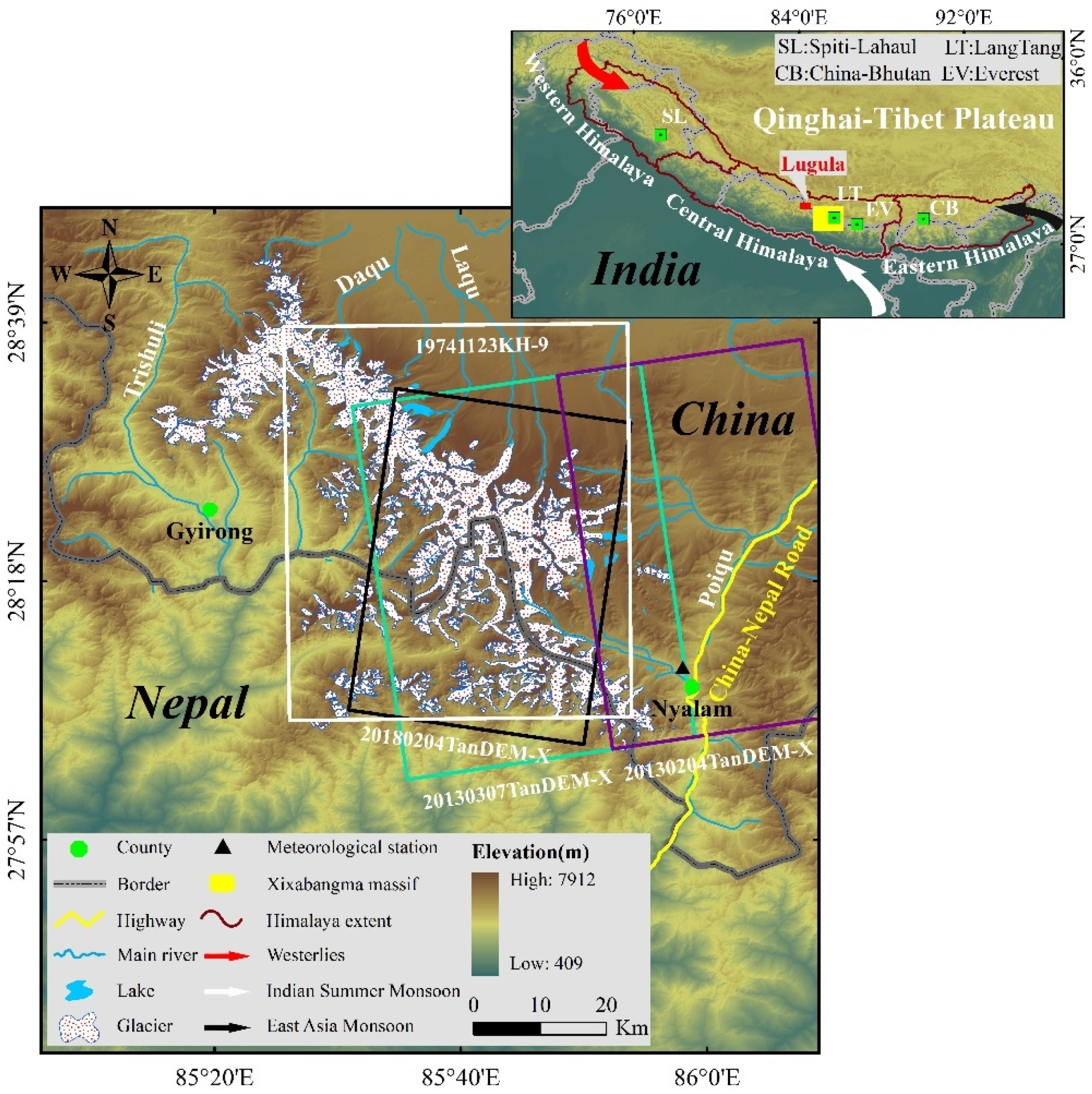
2. Study Area
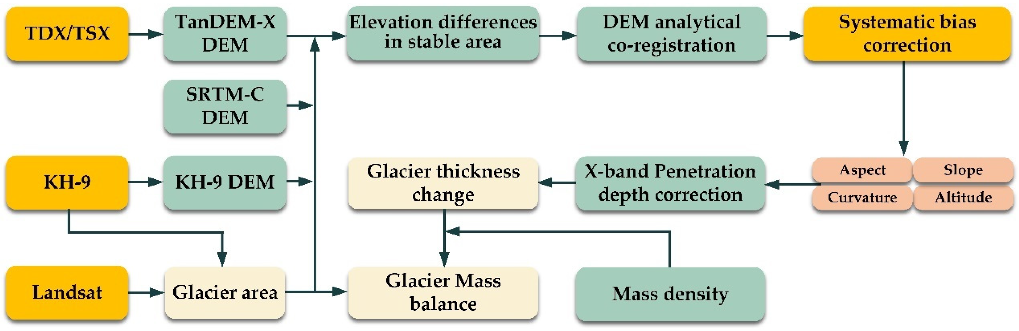
3. Datasets and Methods
3.1. Generation of KH-9 DEM
3.2. Generation of TanDEM-X DEM
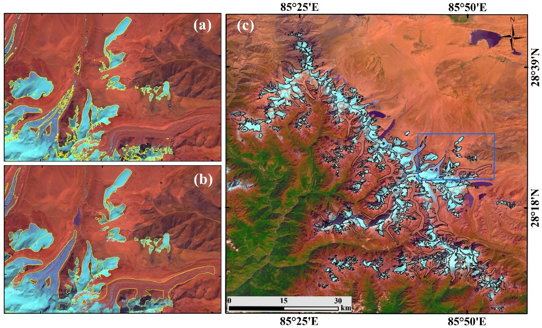
3.3. Delineation of Glacier and Glacial Lake Outlines
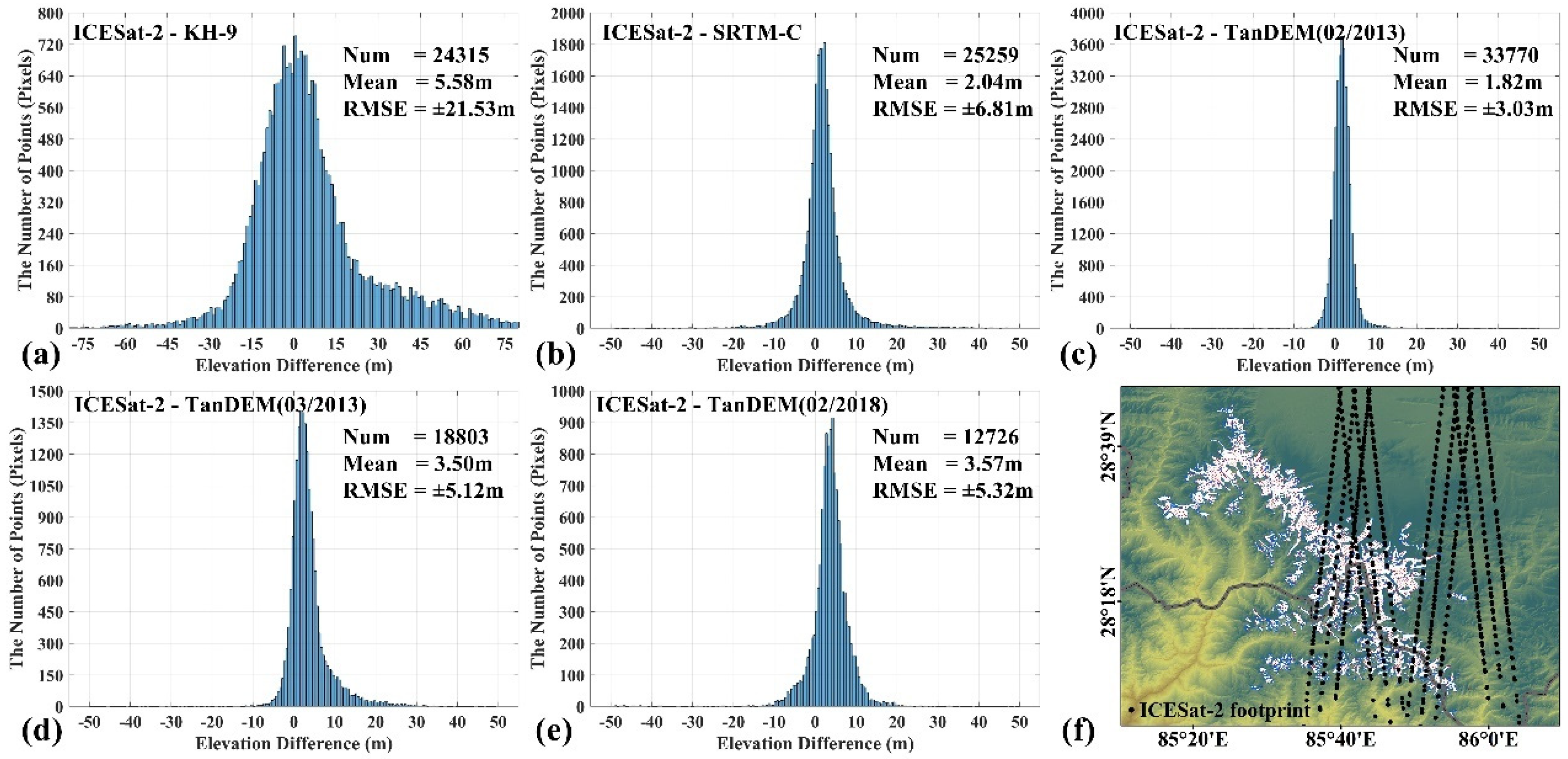
3.4. Evaluation of DEM Accuracy
3.5. Estimation of Changes in Glacier Thickness
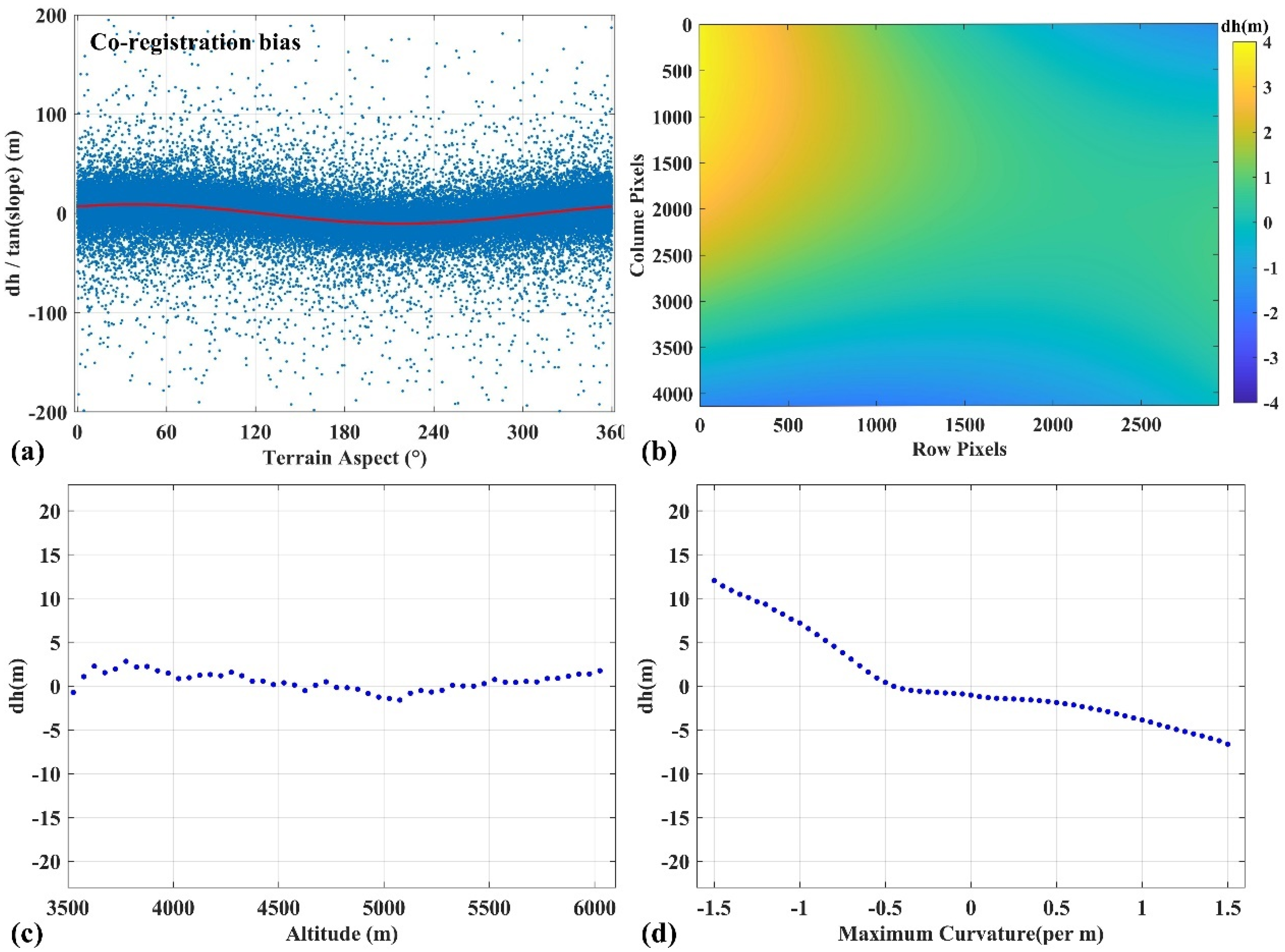
3.5.1. DEM Co-Registration and Systematic Error Correction
3.5.2. Correction of C-Band and X-Band Penetration Effects
3.6. Computation of Glacier Mass Balance
3.7. Uncertainty Analysis
4. Results and Analysis
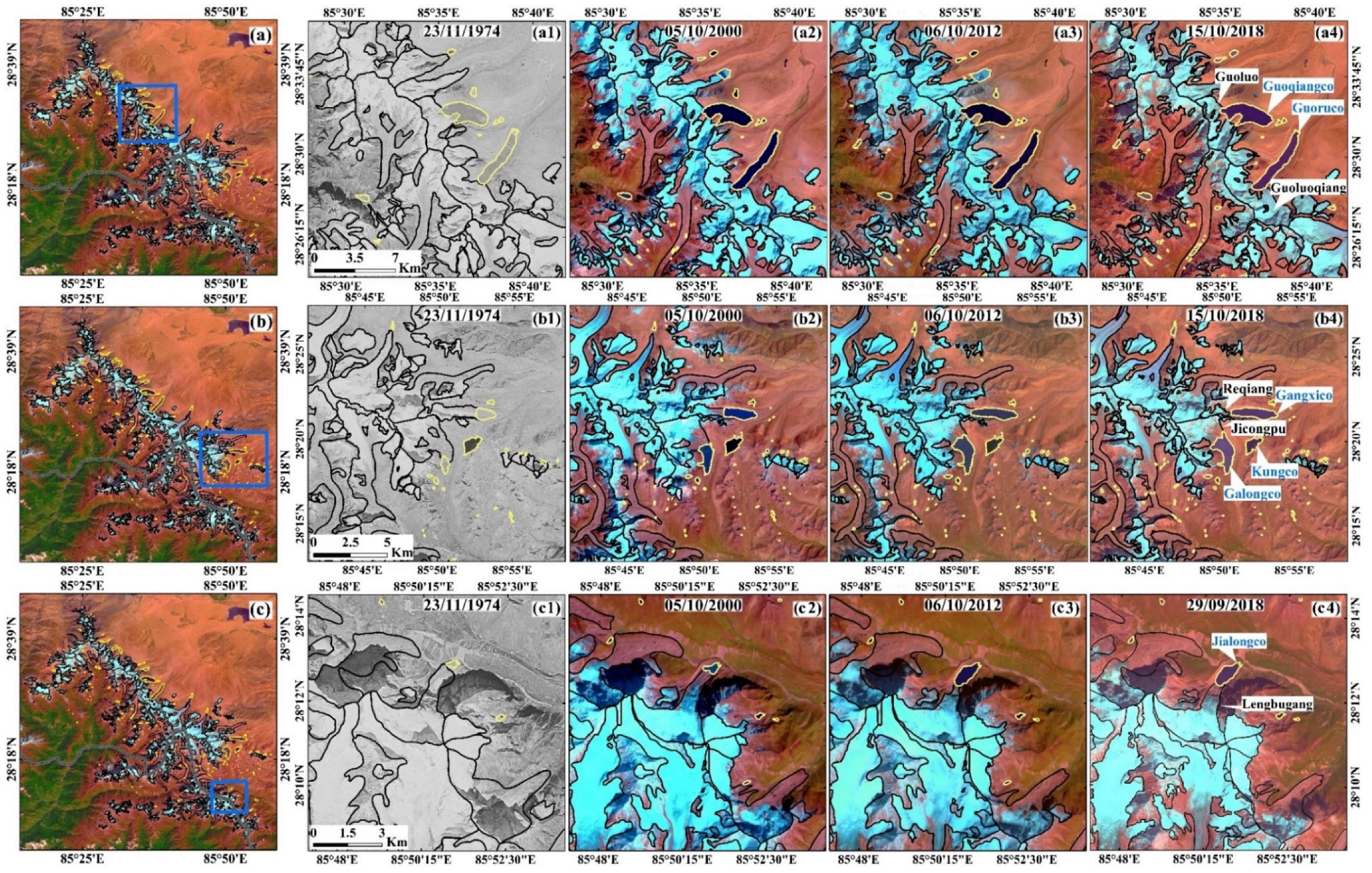
4.1. Changes in Glacier and Glacial Lake Areas during 1974–2018
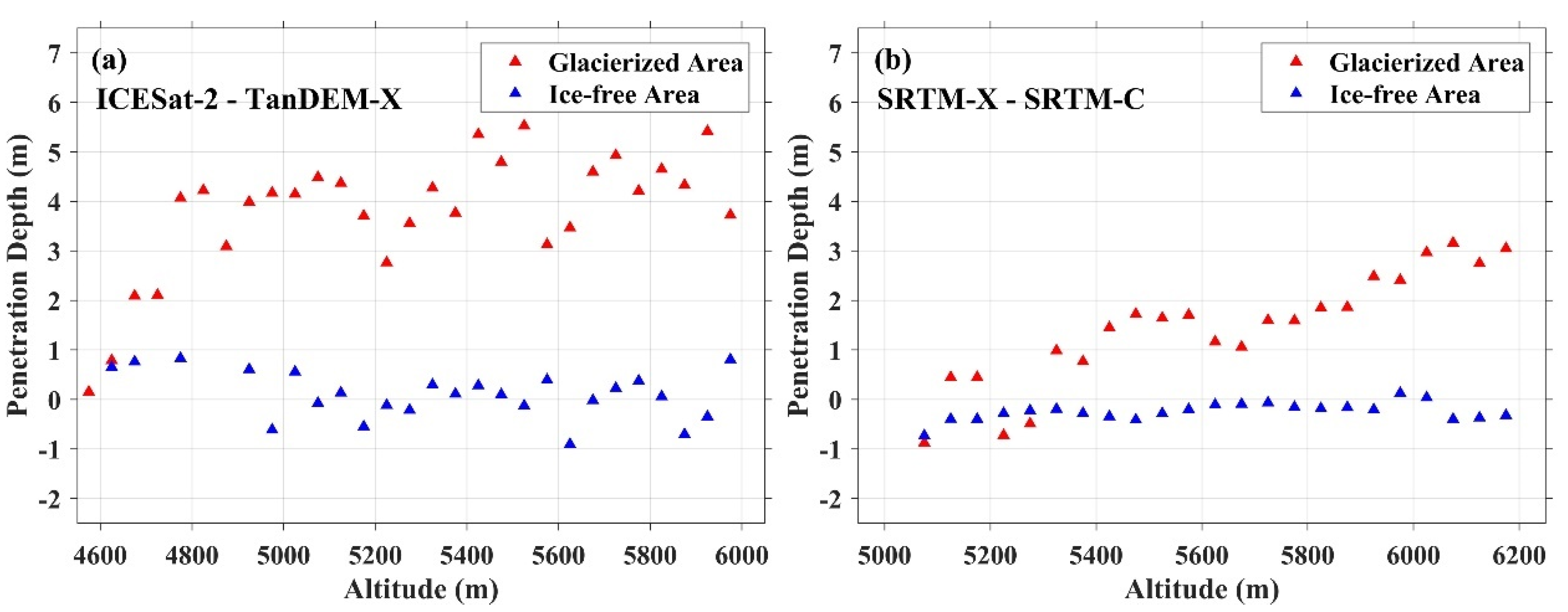
4.2. Radar Penetration Depth over Glaciers
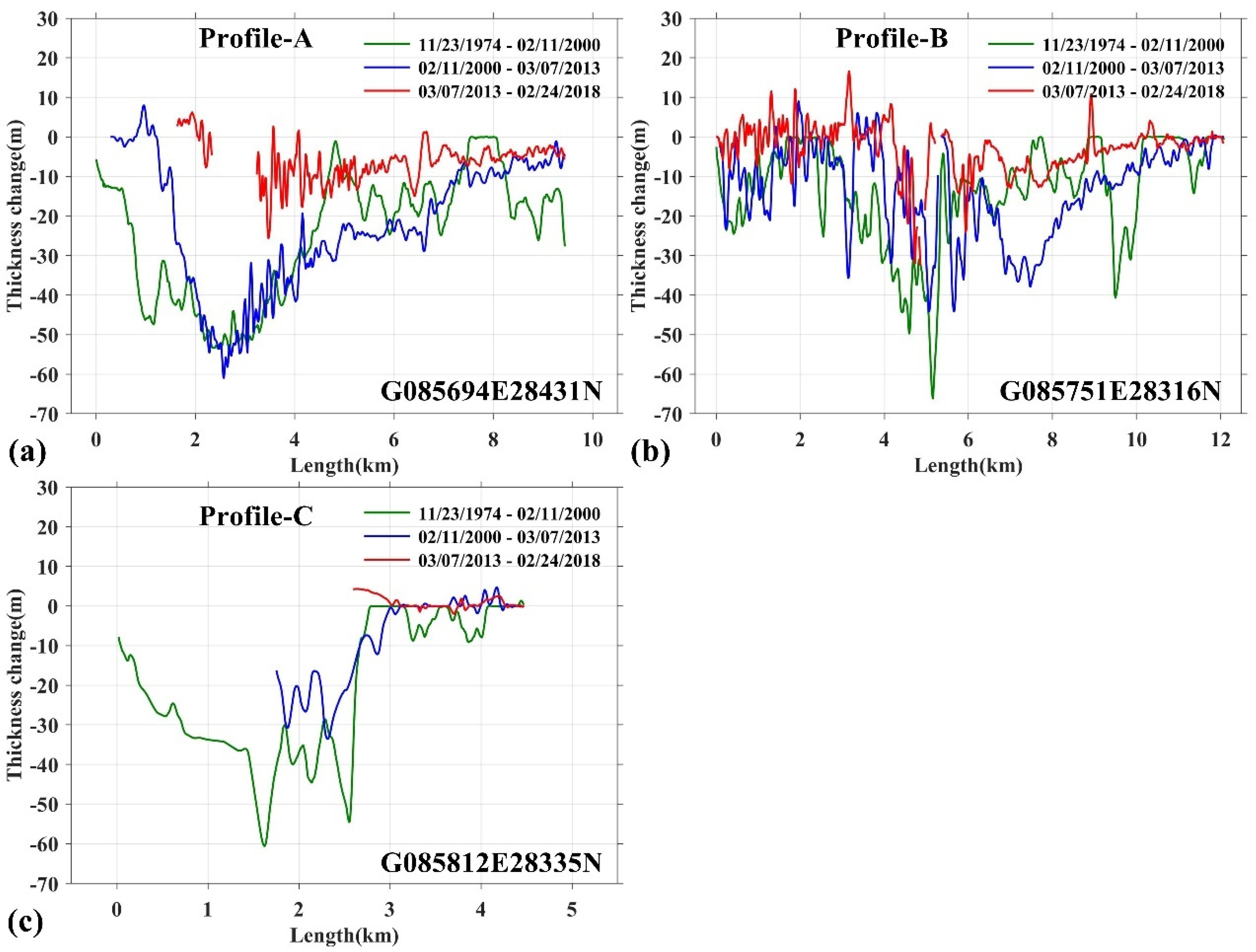
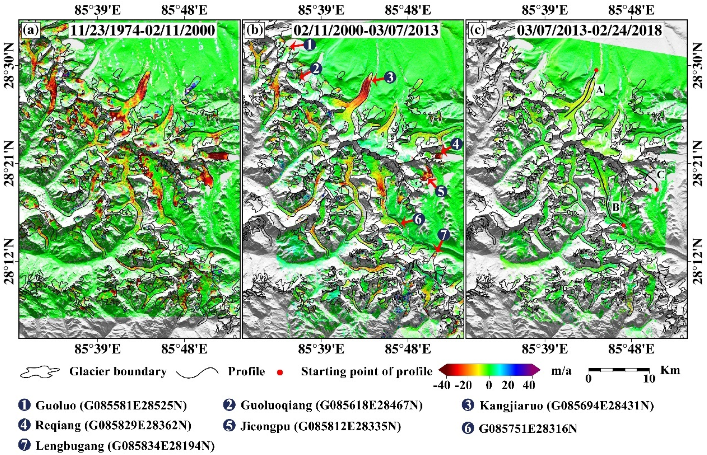
4.3. Changes in Glacier Thickness and Mass Balance
5. Discussion
5.1. Comparison with Previous Glacier Mass Balance Measurements
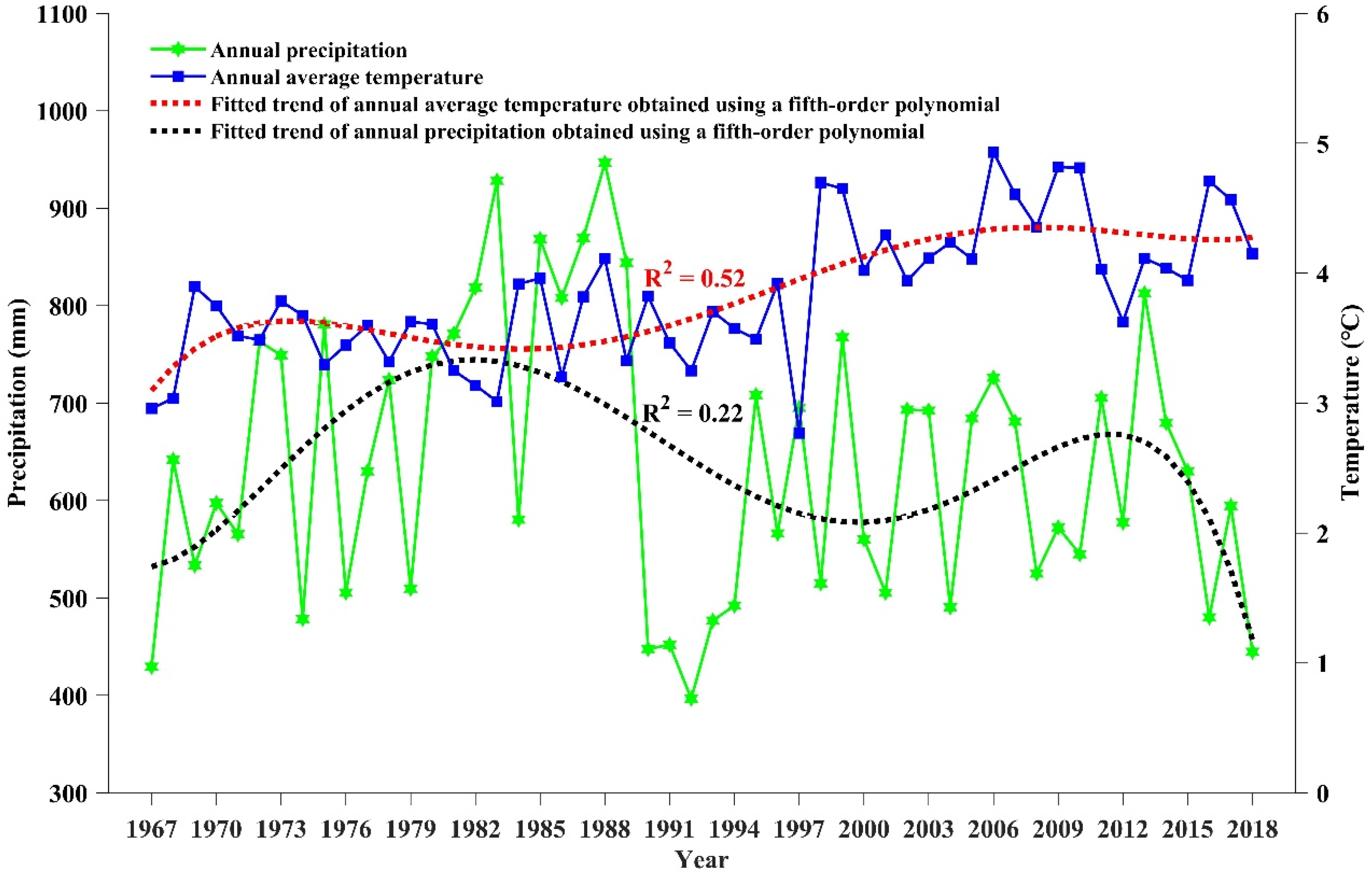
5.2. Relationship between Climate Change and Glacier/Glacial Lake Dynamics
5.3. Outburst Risk of Major Glacial Lakes in the Xixabangma Massif
5.4. Limitations of This Study
6. Conclusions
Author Contributions
Funding
Data Availability Statement
Acknowledgments
Conflicts of Interest
References
- Berthier, E.; Arnaud, Y.; Kumar, R.; Ahmad, S.; Wagnon, P.; Chevallier, P. Remote sensing estimates of glacier mass balances in the Himachal Pradesh (Western Himalaya, India). Remote Sens. Environ. 2007, 108, 327–338. [Google Scholar] [CrossRef] [Green Version]
- Bhushan, S.; Syed, T.H.; Kulkarni, A.V.; Gantayat, P.; Agarwal, V. Quantifying changes in the Gangotri glacier of central Himalaya: Evidence for increasing mass loss and decreasing velocity. IEEE J. Sel. Top. Appl. Earth Obs. Remote Sens. 2017, 10, 5295–5306. [Google Scholar] [CrossRef]
- Immerzeel, W.W.; Lutz, A.F.; Andrade, M.; Bahl, A.; Biemans, H.; Bolch, T.; Hyde, S.; Brumby, S.; Davies, B.; Elmore, A.C.; et al. Importance and vulnerability of the world’s water towers. Nature 2020, 577, 364–369. [Google Scholar] [CrossRef]
- King, O.; Quincey, D.J.; Carrivick, J.L.; Rowan, A.V. Spatial variability in mass loss of glaciers in the Everest region, central Himalayas, between 2000 and 2015. Cryosphere 2017, 11, 407–426. [Google Scholar] [CrossRef] [Green Version]
- Fischer, M.; Korup, O.; Veh, G.; Walz, A. Controls of outbursts of moraine-dammed lakes in the greater Himalayan region. Cryosphere Discuss. 2020, 2020, 1–32. [Google Scholar]
- Rivera, A.; Casassa, G.; Bamber, J.; Kääb, A. Ice-elevation changes of Glaciar Chico, southern Patagonia, using ASTER DEMs, aerial photographs and GPS data. J. Glaciol. 2005, 51, 105–112. [Google Scholar] [CrossRef] [Green Version]
- Rolstad, C.; Haug, T.; Denby, B. Spatially integrated geodetic glacier mass balance and its uncertainty based on geostatistical analysis: Application to the western Svartisen ice cap, Norway. J. Glaciol. 2009, 55, 666–680. [Google Scholar] [CrossRef] [Green Version]
- Matsuo, K.; Heki, K. Time-variable ice loss in Asian high mountains from satellite gravimetry. Earth Planet. Sci. Lett. 2010, 290, 30–36. [Google Scholar] [CrossRef]
- Bolch, T.; Kulkarni, A.; Kääb, A.; Huggel, C.; Paul, F.; Cogley, J.G.; Frey, H.; Kargel, J.S.; Fujita, K.; Scheel, M.; et al. The state and fate of Himalayan glaciers. Science 2012, 336, 310–314. [Google Scholar] [CrossRef] [Green Version]
- Akhtar, M.; Ahmad, N.; Booij, M. The impact of climate change on the water resources of Hindukush–Karakorum–Himalaya region under different glacier coverage scenarios. J. Hydrol. 2008, 355, 148–163. [Google Scholar] [CrossRef]
- Scherler, D.; Bookhagen, B.; Strecker, M.R. Spatially variable response of Himalayan glaciers to climate change affected by debris cover. Nat. Geosci. 2011, 4, 156–159. [Google Scholar] [CrossRef]
- Rowan, A.V.; Egholm, D.L.; Quincey, D.J.; Glasser, N.F. Modelling the feedbacks between mass balance, ice flow and debris transport to predict the response to climate change of debris-covered glaciers in the Himalaya. Earth Planet. Sci. Lett. 2015, 430, 427–438. [Google Scholar] [CrossRef] [Green Version]
- King, O.; Bhattacharya, A.; Bhambri, R.; Bolch, T. Glacial lakes exacerbate Himalayan glacier mass loss. Sci. Rep. 2019, 9, 1–9. [Google Scholar] [CrossRef] [Green Version]
- Nie, Y.; Liu, Q.; Wang, J.; Zhang, Y.; Sheng, Y.; Liu, S. An inventory of historical glacial lake outburst floods in the Himalayas based on remote sensing observations and geomorphological analysis. Geomorphology 2018, 308, 91–106. [Google Scholar] [CrossRef]
- Chen, X.-Q.; Cui, P.; Li, Y.; Yang, Z.; Qi, Y.-Q. Changes in glacial lakes and glaciers of post-1986 in the Poiqu River basin, Nyalam, Xizang (Tibet). Geomorphology 2007, 88, 298–311. [Google Scholar] [CrossRef]
- Shijin, W.; Shitai, J. Evolution and outburst risk analysis of moraine-dammed lakes in the central Chinese Himalaya. J. Earth Syst. Sci. 2015, 124, 567–576. [Google Scholar] [CrossRef] [Green Version]
- Zhang, G.; Bolch, T.; Allen, S.; Linsbauer, A.; Chen, W.; Wang, W. Glacial lake evolution and glacier–lake interactions in the Poiqu River basin, central Himalaya, 1964–2017. J. Glaciol. 2019, 65, 347–365. [Google Scholar] [CrossRef] [Green Version]
- Vincent, C.; Ramanathan, A.; Wagnon, P.; Dobhal, D.P.; Linda, A.; Berthier, E.; Sharma, P.; Arnaud, Y.; Azam, M.F.; Jose, P.G.; et al. Balanced conditions or slight mass gain of glaciers in the Lahaul and Spiti region (northern India, Himalaya) during the nineties preceded recent mass loss. Cryosphere 2013, 7, 569–582. [Google Scholar] [CrossRef] [Green Version]
- Azam, M.F.; Ramanathan, A.; Wagnon, P.; Vincent, C.; Linda, A.; Berthier, E.; Sharma, P.; Mandal, A.; Angchuk, T.; Singh, V.; et al. Meteorological conditions, seasonal and annual mass balances of Chhota Shigri Glacier, western Himalaya, India. Ann. Glaciol. 2016, 57, 328–338. [Google Scholar] [CrossRef] [Green Version]
- Vijay, S.; Braun, M. Elevation change rates of glaciers in the Lahaul-Spiti (Western Himalaya, India) during 2000–2012 and 2012–2013. Remote Sens. 2016, 8, 1038. [Google Scholar] [CrossRef] [Green Version]
- Mukherjee, K.; Bhattacharya, A.; Pieczonka, T.; Ghosh, S.; Bolch, T. Glacier mass budget and climate reanalysis data indicate a climatic shift around 2000 in Lahaul-Spiti, western Himalaya. Clim. Chang. 2018, 148, 219–233. [Google Scholar] [CrossRef]
- Gardelle, J.; Berthier, E.; Arnaud, Y.; Kääb, A. Region-wide glacier mass balances over the Pamir-Karakoram-Himalaya during 1999–2011. Cryosphere 2013, 7, 1263–1286. [Google Scholar] [CrossRef] [Green Version]
- Maurer, J.M.; Rupper, S.B.; Schaefer, J.M. Quantifying ice loss in the eastern Himalayas since 1974 using declassified spy satellite imagery. Cryosphere 2016, 10, 2203–2215. [Google Scholar] [CrossRef] [Green Version]
- Bolch, T.; Pieczonka, T.; Benn, D.I. Multi-decadal mass loss of glaciers in the Everest area (Nepal Himalaya) derived from stereo imagery. Cryosphere 2011, 5, 349–358. [Google Scholar] [CrossRef] [Green Version]
- Pellicciotti, F.; Stephan, C.; Miles, E.; Herreid, S.; Immerzeel, W.W.; Bolch, T. Mass-balance changes of the debris-covered glaciers in the Langtang Himal, Nepal, from 1974 to 1999. J. Glaciol. 2015, 61, 373–386. [Google Scholar] [CrossRef] [Green Version]
- Lamsal, D.; Fujita, K.; Sakai, A. Surface lowering of the debris-covered area of Kanchenjunga Glacier in the eastern Nepal Himalaya since 1975, as revealed by Hexagon KH-9 and ALOS satellite observations. Cryosphere 2017, 11, 2815–2827. [Google Scholar] [CrossRef] [Green Version]
- Chen, X.; Cui, P.; Yang., Z.; Qi, Y. Debris flows of Chongdui Gully in Nyalam County, 2002: Cause and control. J. Glaciol. Geocryol. 2006, 28, 776–781. (In Chinese) [Google Scholar]
- Kargel, J.S.; Leonard, G.J.; Shugar, D.H.; Haritashya, U.K.; Bevington, A.; Fielding, E.J.; Fujita, K.; Geertsema, M.; Miles, E.S.; Steiner, J.; et al. Geomorphic and geologic controls of geohazards induced by Nepals 2015 Gorkha earthquake. Science 2015, 351, aac8353. [Google Scholar] [CrossRef] [Green Version]
- Surazakov, A.; Aizen, V. Positional accuracy evaluation of declassified hexagon KH-9 mapping camera imagery. Photogramm. Eng. Remote. Sens. 2010, 76, 603–608. [Google Scholar] [CrossRef] [Green Version]
- Zhang, X.; Zhou, J.; Liu, Z. DEM extraction and precision evaluation of mountain glaciers in the Qinghai-Tibet Plateau based on KH-data: Take the Purog Kangri Glacier and the Jiong Glacier as example. J. Glaciol. Geocryol. 2019, 41, 27–35. (In Chinese) [Google Scholar]
- Pieczonka, T.; Bolch, T.; Junfeng, W.; Shiyin, L. Heterogeneous mass loss of glaciers in the Aksu-Tarim Catchment (Central Tien Shan) revealed by 1976 KH-9 hexagon and 2009 SPOT-5 stereo imagery. Remote Sens. Environ. 2013, 130, 233–244. [Google Scholar] [CrossRef] [Green Version]
- Wang, Y.; Li, J.; Wu, L.; Guo, L.; Li, J. Using remote sensing images to monitor the glacier changes in Qilian Mountains during 1987–2018 and analyzing the impact factors. J. Glaciol. Geocryol. 2020, 42, 344–356. (In Chinese) [Google Scholar]
- Andreassen, L.M.; Paul, F.; Kääb, A.; Hausberg, J.E. Landsat-derived glacier inventory for Jotunheimen, Norway, and deduced glacier changes since the 1930s. Cryosphere 2008, 2, 131–145. [Google Scholar] [CrossRef] [Green Version]
- Kwok, R.; Cunningham, G.F.; Zwally, H.J.; Yi, D. ICESat over Arctic sea ice: Interpretation of altimetric and reflectivity profiles. J. Geophys. Res. Oceans 2006, 111, C06006. [Google Scholar] [CrossRef]
- Smith, B.; Fricker, H.A.; Holschuh, N.; Gardner, A.; Adusumilli, S.; Brunt, K.M.; Csatho, B.; Harbeck, K.; Huth, A.; Neumann, T.; et al. Land ice height-retrieval algorithm for NASA’s ICESat-2 photon-counting laser altimeter. Remote Sens. Environ. 2019, 233, 111352. [Google Scholar] [CrossRef] [Green Version]
- Nuth, C.; Kääb, A. Co-registration and bias corrections of satellite elevation data sets for quantifying glacier thickness change. Cryosphere 2011, 5, 271–290. [Google Scholar] [CrossRef] [Green Version]
- Li, Z.-W.; Li, J.; Ding, X.-L.; Wu, L.; Ke, L.-H.; Hu, J.; Xu, B.; Peng, F. Anomalous glacier changes in the southeast of Tuomuer-khan Tengri Mountain ranges, central Tianshan. J. Geophys. Res. Atmos. 2018, 123, 6840–6863. [Google Scholar] [CrossRef]
- Berthier, E.; Arnaud, Y.; Baratoux, D.; Vincent, C.; Rémy, F. Recent rapid thinning of the “Mer de Glace” glacier derived from satellite optical images. Geophys. Res. Lett. 2004, 31, L17401. [Google Scholar] [CrossRef] [Green Version]
- Guo, L.; Li, J.; Wu, L.; Li, Z.; Liu, Y.; Li, X.; Miao, Z.; Wang, W. Investigating the recent surge in the Monomah Glacier, Central Kunlun Mountain range with multiple sources of remote sensing data. Remote Sens. 2020, 12, 966. [Google Scholar] [CrossRef] [Green Version]
- Höhle, J.; Höhle, M. Accuracy assessment of digital elevation models by means of robust statistical methods. ISPRS J. Photogramm. Remote Sens. 2009, 64, 398–406. [Google Scholar] [CrossRef] [Green Version]
- Huss, M. Density assumptions for converting geodetic glacier volume change to mass change. Cryosphere 2013, 7, 877–887. [Google Scholar] [CrossRef] [Green Version]
- Fujita, K.; Sakai, A.; Nuimura, T.; Yamaguchi, S.; Sharma, R.R. Recent changes in Imja Glacial Lake and its damming moraine in the Nepal Himalaya revealed by in situ surveys and multi-temporal ASTER imagery. Environ. Res. Lett. 2009, 4, 045205. [Google Scholar] [CrossRef]
- Li, J.; Li, Z.-W.; Hu, J.; Wu, L.-X.; Li, X.; Guo, L.; Liu, Z.; Miao, Z.-L.; Wang, W.; Chen, J.-L. Investigating the bias of TanDEM-X digital elevation models of glaciers on the Tibetan Plateau: Impacting factors and potential effects on geodetic mass-balance measurements. J. Glaciol. 2021, 2021, 1–14. [Google Scholar] [CrossRef]
- Dehecq, A.; Millan, R.; Berthier, E.; Gourmelen, N.; Trouve, E.; Vionnet, V. Elevation changes inferred from TanDEM-X data over the Mont-Blanc area: Impact of the X-band interferometric bias. IEEE J. Sel. Top. Appl. Earth Obs. Remote Sens. 2016, 9, 3870–3882. [Google Scholar] [CrossRef] [Green Version]
- Lambrecht, A.; Mayer, C.; Wendt, A.; Floricioiu, D.; Völksen, C. Elevation change of Fedchenko Glacier, Pamir Mountains, from GNSS field measurements and TanDEM-X elevation models, with a focus on the upper glacier. J. Glaciol. 2018, 64, 637–648. [Google Scholar] [CrossRef] [Green Version]
- Zhou, Y.; Li, Z.; Li, J.; Zhao, R.; Ding, X. Glacier mass balance in the Qinghai–Tibet Plateau and its surroundings from the mid-1970s to 2000 based on Hexagon KH-9 and SRTM DEMs. Remote Sens. Environ. 2018, 210, 96–112. [Google Scholar] [CrossRef]
- Raina, V.K. Himalayan Glaciers: A State-Of-Art Review of Glacial Studies, Glacial Retreat and Climate Change; Ministry of Environment and Forests, Government of India: New Delhi, India, 2009; p. 43.
- Wu, K.; Liu, S.; Jiang, Z.; Xu, J.; Wei, J.; Guo, W. Recent glacier mass balance and area changes in the Kangri Karpo Mountains from DEMs and glacier inventories. Cryosphere 2018, 12, 103–121. [Google Scholar] [CrossRef] [Green Version]
- Kääb, A.; Berthier, E.; Nuth, C.; Gardelle, J.; Arnaud, Y. Contrasting patterns of early twenty-first-century glacier mass change in the Himalayas. Nature 2012, 488, 495–498. [Google Scholar] [CrossRef]
- Brun, F.; Berthier, E.; Wagnon, P.; Kääb, A.; Treichler, D. A spatially resolved estimate of High Mountain Asia glacier mass balances from 2000 to 2016. Nat. Geosci. 2017, 10, 668–673. [Google Scholar] [CrossRef]
- Veettil, B.K.; Kamp, U. Glacial lakes in the Andes under a changing climate: A review. J. Earth Sci. 2021, 32, 1–19. [Google Scholar] [CrossRef]
- Wang, W.; Yao, T.; Gao, Y.; Yang, X.; Kattel, D.B. A first-order method to identify potentially dangerous glacial lakes in a region of the Southeastern Tibetan Plateau. Mt. Res. Dev. 2011, 31, 122. [Google Scholar] [CrossRef]
- Wang, X.; Liu, S.; Ding, Y.; Guo, W.; Jiang, Z.; Lin, J.; Han, Y. An approach for estimating the breach probabilities of moraine-dammed lakes in the Chinese Himalayas using remote-sensing data. Nat. Hazards Earth Syst. Sci. 2012, 12, 3109–3122. [Google Scholar] [CrossRef] [Green Version]
- Bolch, T.; Peters, J.; Yegorov, A.; Pradhan, B.; Buchroithner, M.; Blagoveshchensky, V. Identification of potentially dangerous glacial lakes in the northern Tien Shan. Nat. Hazards 2011, 59, 1691–1714. [Google Scholar] [CrossRef] [Green Version]


| Reference | Location | Glacier Area (km2) | Data | Period | Mass Balance (m w.e./a) |
|---|---|---|---|---|---|
| [1] | Spiti-Lahaul | 608.8 | SRTM-C DEM–SPOT5 DEM | 1999–2004 | −0.7~−0.85 |
| [18] | Chhota-Shigri | 15.7 | SRTM-C DEM–SPOT5 DEM | 1999–2011 | −0.39 ± 0.15 |
| [19] | Chhota-Shigri | 15.5 | Field Measurements–SPOT5 DEM | 2002–2014 | −0.56 ± 0.40 |
| Pleiades DEM–SPOT5 DEM | 2005–2014 | −0.34 ± 0.24 | |||
| [20] | Spiti-Lahaul | 1711.9 | SRTM-C DEM–TanDEM-X DEM | 2000–2012 | −0.53 ± 0.37 |
| [21] | Spiti-Lahaul | 350.3 | KH-4B DEM–SRTM-C DEM | 1971–1999 | −0.07 ± 0.10 |
| SRTM-C DEM–ASTER/Cartosat-1 DEM | After 2000 | −0.30 ± 0.10 | |||
| [22] | Bhutan | 1367.1 | SRTM-C DEM–SPOT5 DEM | 2000–2011 | −0.22 ± 0.13 |
| [23] | China-Bhutan | 365 | KH-9 DEM–ASTER DEM | 1974–2006 | −0.17 ± 0.05 |
| [24] | Everest | 46.9 | KH-4B DEM–Cartosat-1 DEM | 1970–2007 | −0.32 ± 0.08 |
| 49.6 | Cartosat-1 DEM–ASTER DEM | 2002–2007 | −0.79 ± 0.52 | ||
| [22] | West Nepal | 890.4 | SRTM-C DEM–SPOT5 DEM | 2000–2011 | −0.32 ± 0.14 |
| [25] | Langtang | 94.9 | KH-9 DEM–SRTM-C DEM | 1974–2000 | −0.32 ± 0.18 |
| [26] | Kanchenjunga | 60.5 | KH-9 DEM–PRISM DEM | 1975–2010 | −0.18 ± 0.17 |
| [4] | Everest | 706.6 | SRTM-C DEM–Worldview DEM | 2000–2015 | −0.52 ± 0.22 |
| [2] | Gangotri | 122 | SRTM-C DEM–Cartosat-1 DEM | 1999–2014 | −0.55 ± 0.42 |
| Data | Date | Resolution | Product ID | Usage |
|---|---|---|---|---|
| KH-9 stereo image | 23/11/1974 | 7 m | DZB1209-500101L006001 | Glacier/glacial lake outline delineation; DEM extraction |
| DZB1209-500101L007001 | ||||
| Landsat-8 OLI image | 24/10/2018 | 15 m | LC81400412018297LGN00 | Glacier/glacial lake outline delineation |
| 09/11/2018 | LC81400412018313LGN00 | |||
| 25/11/2018 | LC81400412018329LGN00 | |||
| Landsat-7 ETM+ image | 06/10/2012 | LE71410402012280PFS00 | ||
| 22/10/2012 | LE71410402012296PFS00 | |||
| 07/11/2012 | LE71410402012312PFS00 | |||
| 05/10/2000 | LE71410402000279SGS00 | Glacier/glacial lake outline delineation; horizontal reference for DEM extraction | ||
| 22/11/2000 | LE71410392000327EDC00 | |||
| LE71410402000327EDC00 | ||||
| LE71410412000327EDC00 | ||||
| Landsat-5 TM image | 13/10/2000 | 30 m | LT51410402000287BKT00 | Glacier/glacial lake outline delineation |
| 16/12/2000 | LT51410402000351BKT00 | |||
| TanDEM-X CoSSC image | 07/03/2013 | 1.36 m × 1.85 m (Range × Azimuth) | TDM1_SAR_COS_BIST_SM_S_SRA 20130307T121856_20130307T121904 | DEM extraction |
| 24/02/2013 | TDM1_SAR_COS_BIST_SM_S_SRA 20130224T121856_20130224T121904 | |||
| 24/02/2018 | TDM1_SAR_COS_BIST_SM_S_SRA 20180224T001328_20180224T001335 | |||
| SRTM-C DEM | 11/02/2000 | 30 m | ------ | Historical elevation; horizontal reference for DEM extraction |
| ICESat-2/ATLAS ATL06 product | 26/10/2018 | Point | ATL06_20181026091136_04240102_002 | DEM accuracy assessment |
| 10/11/2018 | ATL06_20181110202842_06600106_002 | |||
| 27/12/2018 | ATL06_20181227061521_13690102_002 | |||
| 11/01/2019 | ATL06_20190111173213_02180206_002 | |||
| 27/12/2018 | ATL06_20181227061521_13690102_002 | X-band penetration depth estimation | ||
| 09/02/2019 | ATL06_20190209160826_06600206_002 | |||
| Meteorological data | 1967–2018 | Station | ------ | Climate change |
| Period | Raw Elevation Difference | Corrected Elevation Difference | Improvement of NMAD | ||
|---|---|---|---|---|---|
| Mean | NMAD | Mean | NMAD | ||
| 1974–2000 | −1.18 | 15.63 | 0.22 | 12.17 | 22.14% |
| 2000–2013 | 0.01 | 5.25 | −0.05 | 3.58 | 31.81% |
| 2013–2018 | −0.47 | 3.33 | 0.01 | 2.32 | 30.33% |
| Glacier (GLIMS ID) | Glacial Lake | Area (km2) | |||||||
|---|---|---|---|---|---|---|---|---|---|
| 1974 | 2000 | 2012 | 2018 | ||||||
| Glacier | Lake | Glacier | Lake | Glacier | Lake | Glacier | Lake | ||
| Guoluo (G085581E28525N) | Guoqiangco | 8.58 ±0.12 | 4.93 ±0.08 | 7.59 ±0.37 | 5.07 ±0.19 | 7.36 ±0.18 | 5.21 ±0.10 | 7.09 ±0.18 | 5.34 ±0.10 |
| Guoluoqiang (G085618E28467N) | Guoruco | 14.31 ±0.15 | 4.16 ±0.09 | 13.13 ±0.39 | 4.67 ±0.22 | 12.93 ±0.20 | 4.74 ±0.11 | 12.80 ±0.21 | 4.77 ±0.11 |
| Reqiang (G085829E28362N) | Gangxico | 5.74 ±0.13 | 1.99 ±0.04 | 4.46 ±0.25 | 3.50 ±0.13 | 3.35 ±0.11 | 4.49 ±0.09 | 2.51 ±0.11 | 4.52 ±0.09 |
| Jicongpu (G085812E28335N) | Galongco | 19.79 ±0.21 | 1.13 ±0.03 | 17.28 ±0.39 | 3.24 ±0.17 | 15.47 ±0.19 | 5.05 ±0.10 | 14.78 ±0.20 | 5.35 ±0.11 |
| Lengbugang (G085834E28194E) | Jialongco | 5.66 ±0.10 | 0.11 ±0.01 | 5.08 ±0.19 | 0.20 ±0.03 | 4.53 ±0.08 | 0.57 ±0.03 | 4.31 ±0.09 | 0.59 ±0.03 |
| ------ | Kungco | ------ | 2.22 ±0.05 | ------ | 2.18 ±0.09 | ------ | 2.04 ±0.05 | ------ | 1.92 ±0.05 |
| Whole region | Whole region | 954.01 ±18.51 | 20.90 ±0.81 | 830.03 ±43.39 | 30.40 ±3.22 | 786.57 ±21.22 | 36.70 ±1.86 | 752.46 ±21.51 | 38.71 ±1.93 |
| Glacier Name (GLIMS ID) | Thickness Change (m/a) | ||
|---|---|---|---|
| 1974–2000 | 2000–2013 | 2013–2018 | |
| Kangjiaruo (G085694E28431N) | −0.57 ± 0.06 | −0.86 ± 0.04 | −0.93 ± 0.07 |
| ------ (G085751E28316N) | −0.28 ± 0.06 | −0.63 ± 0.04 | −0.32 ± 0.07 |
| Reqiang (G085829E28362N) | −1.09 ± 0.12 | −1.99 ± 0.13 | ------ |
| Jicongpu (G085812E28335N) | −0.42 ± 0.08 | −0.95 ± 0.08 | 0.12 ± 0.20 |
| Lengbugang G085834E28194N | −0.12 ± 0.14 | −0.31 ± 0.12 | −0.33 ± 0.29 |
| Guoluoqiang (G085618E28467N) | −0.05 ± 0.09 | −0.12 ± 0.08 | ------ |
| Guoluo (G085581E28525N) | −0.14 ± 0.12 | −0.27 ± 0.11 | ------ |
Publisher’s Note: MDPI stays neutral with regard to jurisdictional claims in published maps and institutional affiliations. |
© 2021 by the authors. Licensee MDPI, Basel, Switzerland. This article is an open access article distributed under the terms and conditions of the Creative Commons Attribution (CC BY) license (https://creativecommons.org/licenses/by/4.0/).
Share and Cite
Wang, Y.; Li, J.; Wu, L.; Guo, L.; Hu, J.; Zhang, X. Estimating the Changes in Glaciers and Glacial Lakes in the Xixabangma Massif, Central Himalayas, between 1974 and 2018 from Multisource Remote Sensing Data. Remote Sens. 2021, 13, 3903. https://doi.org/10.3390/rs13193903
Wang Y, Li J, Wu L, Guo L, Hu J, Zhang X. Estimating the Changes in Glaciers and Glacial Lakes in the Xixabangma Massif, Central Himalayas, between 1974 and 2018 from Multisource Remote Sensing Data. Remote Sensing. 2021; 13(19):3903. https://doi.org/10.3390/rs13193903
Chicago/Turabian StyleWang, Yingzheng, Jia Li, Lixin Wu, Lei Guo, Jun Hu, and Xin Zhang. 2021. "Estimating the Changes in Glaciers and Glacial Lakes in the Xixabangma Massif, Central Himalayas, between 1974 and 2018 from Multisource Remote Sensing Data" Remote Sensing 13, no. 19: 3903. https://doi.org/10.3390/rs13193903
APA StyleWang, Y., Li, J., Wu, L., Guo, L., Hu, J., & Zhang, X. (2021). Estimating the Changes in Glaciers and Glacial Lakes in the Xixabangma Massif, Central Himalayas, between 1974 and 2018 from Multisource Remote Sensing Data. Remote Sensing, 13(19), 3903. https://doi.org/10.3390/rs13193903