Abstract
Leaf chlorophyll content (LCC) is one of the most important factors affecting photosynthetic capacity and nitrogen status, both of which influence crop harvest. However, the development of rapid and nondestructive methods for leaf chlorophyll estimation is a topic of much interest. Hence, this study explored the use of the machine learning approach to enhance the estimation of leaf chlorophyll from spectral reflectance data. The objective of this study was to evaluate four different approaches for estimating the LCC of apple tree leaves at five growth stages (the 1st, 2nd, 3rd, 4th and 5th growth stages): (1) univariate linear regression (ULR); (2) multivariate linear regression (MLR); (3) support vector regression (SVR); and (4) random forest (RF) regression. Samples were collected from the leaves on the eastern, western, southern and northern sides of apple trees five times (1st, 2nd, 3rd, 4th and 5th growth stages) over three consecutive years (2016–2018), and experiments were conducted in 10–20-year-old apple tree orchards. Correlation analysis results showed that LCC and ST, LCC and vegetation indices (VIs), and LCC and three edge parameters (TEP) had high correlations with the first-order differential spectrum (FODS) (0.86), leaf chlorophyll index (LCI) (0.87), and (SDr − SDb)/ (SDr + SDb) (0.88) at the 3rd, 3rd, and 4th growth stages, respectively. The prediction models of different growth stages were relatively good. The MLR and SVR models in the LCC assessment of different growth stages only reached the highest R2 values of 0.79 and 0.82, and the lowest RMSEs were 2.27 and 2.02, respectively. However, the RF model evaluation was significantly better than above models. The R2 value was greater than 0.94 and RMSE was less than 1.37 at different growth stages. The prediction accuracy of the 1st growth stage (R2 = 0.96, RMSE = 0.95) was best with the RF model. This result could provide a theoretical basis for orchard management. In the future, more models based on machine learning techniques should be developed using the growth information and physiological parameters of orchards that provide technical support for intelligent orchard management.
1. Introduction
The Leaf chlorophyll content (LCC) represents the photosynthetic rate, nitrogen content and health status of crops; it is also an indicator of the nutrient status of crop plants and the degree of senescence [1]. It has significance for crop growth monitoring, nutrient content monitoring, quality evaluation and yield estimation [2]. LCC is essential because the nutritional status of crops determines yield and food safety. In the past, traditional methods of its calculation were time-consuming, laborious, and destructive to leaves [3]. Therefore, the accurate estimation of LCC is an important challenge that urgently needs to be addressed.
In recent years, hyperspectral remote sensing (HRS) has become a major development trend in monitoring the chlorophyll content of vegetation due to its high spectral resolution, simplicity, effectiveness, and non-destructiveness [1,4,5]. This method provides an effective means for research on the chlorophyll content of crops and the implementation of precision agriculture. The spectral indices captured by hyperspectral sensors are considered to be quantitative indicators of vegetation vigor [6], and continuous narrow bands have the potential to identify regions sensitive to specific crop parameters. It is well known that the spectral properties of crop leaves are controlled by surface characteristics, internal structure, and concentration of biochemical constituents [7]. Vegetation indices (VIs) have been derived from different mathematical combinations (simple ratios and normalized difference, etc.) of spectral bands to help indicate plant features. Vegetation indices have been used to detect the seasonal variability of LCC, which has been widely used in precision agriculture and crop phenotyping [8,9,10].
Recently, machine-learning techniques have been widely used to build predictive models with improved prediction accuracy. Shah et al. reported that the RF method could better reduce the root mean square error (RMSE) than standard linear regression [8]. Li et al. showed that support vector machine regression (SVMR) methods could better estimate chlorophyll content than the back-propagation neural network (BPNN) method [11]. There is not only a linear relationship between crop physiological parameters and the spectrum but also a nonlinear relationship. Machine learning technology has been extensively applied for crop LCC [8], leaf nitrogen concentration (N) [12], and leaf area index (LAI) [13] estimation.
Apple trees are perennials, and their phenotypic structure and growth characteristics are different from those of field crops, causing large differences in spectral response characteristics. Apple (Malus pumila Mill.) is a kind of deciduous tree, which generally begins to bear fruit 3–5 years after planting, but only apple trees with a fruit age of 10–20 years are in the full fruit period. The chlorophyll content of apple tree leaves varies with changes in different apple phenology phases, leading to different leaf photosynthetic rates at different growth stages, which causes differences in the accumulation of organic matter, which may have an impact on apple yield. According to the annual cycle and law of nutrient transportation, the leaves of the plants gradually turn yellow after apple harvest, so dynamic monitoring the chlorophyll content of apple leaves from the flowering period to the harvest period has great significance [11,14]. Many researchers have performed LCC evaluations with hyperspectral remote sensing technology for a variety of crop species (such as winter wheat, rice and maize) [15,16,17], but estimation of LCC in apple trees is limited, and especially the dynamic monitoring of the chlorophyll content of apple tree leaves in different phenological periods is even rarer. However, China’s apple planting area has grown to account for 42.24% of the world’s total, and it has become the world’s largest apple producer [18]. Shaanxi Province is one of the main apple production areas in China. Apple trees play an indispensable role in the local economy, and nondestructive measurement technology is urgently needed to measure the biochemical parameter indices of orchards. In this context, the accurate estimation of LCC for apple orchards can enable government management departments to formulate appropriate orchard management measures, such as optimizing regional planting structures and fertilization practices. It is imperative, therefore, to find a suitable method for estimating LCC in apple orchards.
In this study, LCC was measured and assessed at five growth stages (1st, 2nd, 3rd, 4th and 5th growth stages) with apple trees of 10–20-year old orchards. The objectives of this study were as follows: (1) to select spectral parameters suitable and applicable for apple tree LCC estimation and (2) to determine the suitability and general applicability of the methods for measuring apple tree LCC.
2. Materials and Methods
2.1. Study Area and Experimental Setup
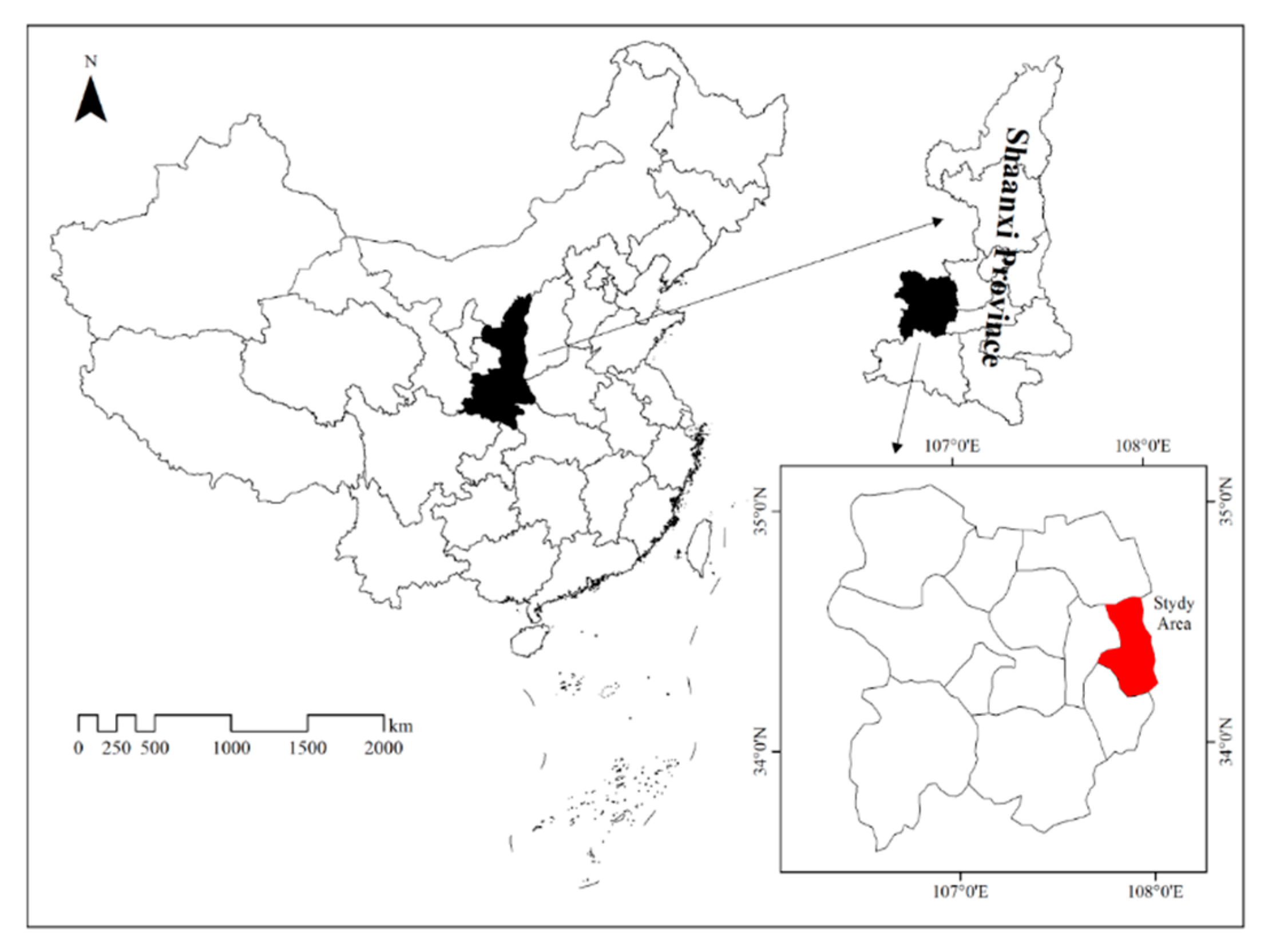
The study was conducted during the 2016–2018 growing seasons (from May to October) in orchards located in Xinglin town, Fufeng County, Shaanxi Province, China (W 107°45′–108°03′, N 34°12′-34°37′) (Figure 1). This region has a temperate, continental, semiarid climate. The average annual precipitation and average annual temperature are 591.9 mm and 12.4 °C, respectively.
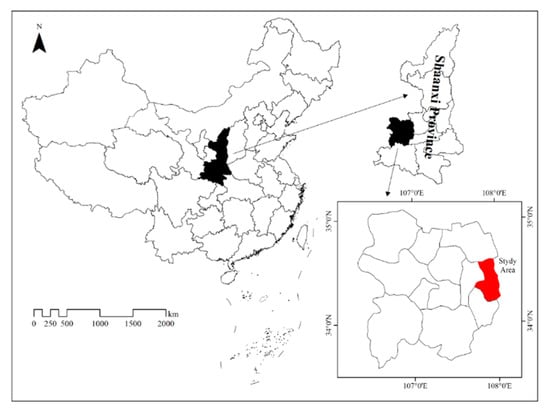
Figure 1.
Study area in this study.
The average height of the apple trees was 2.5 m, the average crown width was 2.5 m, and the spacing was 4 m × 3 m in the apple orchard, which ensured good light conditions and suitable growth temperatures throughout the year. The soil in the apple orchard was a Loess agricultural soil. The basic fertility level of the cultivated soil layer was as follows: the average content of organic matter was 18.65 g/kg, the alkali hydrolyzed nitrogen was 76.68 mg/kg, the available phosphorus was 35.19 mg/kg, and the quick-acting potassium content was 114.91 mg/kg.
From May to October 2016–2018, 17–20 apple trees were selected in 10–20-year-old apple orchards and collected five times (the final flowering stage, fruiting stage, fruit expansion stage, fruit coloring growth stage, and fruit ripening stage) each year. Due to the weather, data from only four growth stages were collected in 2016 (Table 1). Five healthy apple leaves were collected evenly from the upper layer to the lower layer of the canopy in the four directions of the apple tree. A total of 20 apple leaves were collected from each apple tree. The 17 × 20 = 340 (in 2016) and 20 × 20 = 400 (in 2017 and 2018) samples were placed into a freshness protection package, and the packages were then placed in an ice box.

Table 1.
Different growth stages of the samples used in this study.
2.2. Hyperspectral Data Acquisition
A spectroradiometer SVC HR1024i ( Spectra Vista Crop., Poughkeepsie, NY, USA) with 1024 spectral channels and a spectral range of 350–2500 nm was used to measure the spectral reflectance of apple leaves. Spectral resolutions of 3.5, 9.5 and 6.5 nm with spectral ranges of 350–1000, 1000–1890 and 1890–2500 nm [19], respectively, were used. Because the chlorophyll response band to the leaf spectrum is mainly in the visible and reflected infrared bands, the 350–1000 nm band was primarily used for the analysis, and the spectrum was resampled to 2 nm. The spectra of leaves were measured at three randomly selected sample points. Six measurements were conducted for each sample leaf, and 30 spectral measurements (5 × 6) were averaged to represent the reflectance of the leaves. The numbers of spectral samples in this study are shown in Table 1.
2.3. Leaf Chlorophyll Content Measurement
In this study, leaf LCC was determined by collecting samples from point leaves (corresponding to spectral sampling) via a hand-held chlorophyll meter (SPAD-502, Minolta Osaka Company Ltd., Tokyo, Japan) in the laboratory. The chlorophyll meter mainly uses leaf transmittance in the central band of 650 to 940 nm to determine the chlorophyll content [20], and the SPAD value can better reflect the change in leaf greenness. Each sample was collected from the same location on the leaf where the spectral data were sampled. Six measurements were conducted for each sample leaf. The 30 value measurements (5 × 6) were averaged to represent the SPAD values of the leaves.
2.4. Methods
2.4.1. Spectral Transformation (ST)
In this study, the spectral response in Vis-NIR infrared bands at 350–1000 nm was used to estimate the apple tree LCC. All reflectance spectra were resampled at 2 nm spectral intervals [21]. In addition, widely used preprocessing methods were employed in this study, and labeling of the original spectrum (OS) was performed. Then, three types of common STs were used, including a reciprocal transformed spectrum (RS), first-order differential spectrum (FODS) and continuum removal spectrum (CRS) [19,22,23] (Table 2).
2.4.2. Vegetation Indices
The construction of a vegetation index involves the combination of different sensitive bands to eliminate the impact of environmental background effects (such as non-vegetation target soil, water body, etc.) to a certain extent. The vegetation indices evaluated in this study are presented in Table 2. NDVI [24] and mSR705 [25] were selected because they are the earliest and simplest VIs, and their narrowband versions have great potential to improve LCC estimation accuracy. The leaf chlorophyll index (LCI) is a vegetation index involving the red-side band, that uses the spectral reflectance characteristics of the red-side band and the near-infrared band to show differences in chlorophyll content [26]. The ratio vegetation index (RVI) is based on the red and near-infrared bands [27].
2.4.3. Three Edge Parameters
To further study the relationship between spectral data and LCC, the preprocessing of spectral data is required. The “three edge” parameters refer to the relevant variables based on the characteristics of the spectral position, namely, red edge, blue edge and yellow edge [28]. The “three edge” parameters can better reflect the spectral characteristics of green vegetation and are sensitive to LCC changes. Therefore, these parameters can be used as a diagnostic characteristic parameter for LCC. The relevant definitions of the “three edge” parameters are shown in Table 2.

Table 2.
Spectral parameters evaluated in this study.
Table 2.
Spectral parameters evaluated in this study.
| Parameters | Explanation | References |
|---|---|---|
| ST (1) | ||
| OS | Original spectrum | [19] |
| RS | Reciprocal transformed spectrum | [19] |
| FODS | First-order differential spectrum | [19] |
| CRS | Continuum removal spectrum | [19] |
| VIs (2) | ||
| Normalized difference Vegetation index (NDVI) | (R800 − R670)/(R800 + R670) | [24] |
| Ratio vegetation index (RVI) | R765/R720 | [27] |
| Green ratio vegetation index (GRVI) | (R620 − R506)/(R620 + R506) | [29] |
| Photochemical reflectance Index (PRI) | (R570 − R531)/(R570 + R531) | [30] |
| Normalized pigment chlorophyll index (NPCI) | (R642 − R432)/(R642 + R432) | [31] |
| Modified red edge simple ratio index (mSR705) | (R750 − R445)/(R705 − R445) | [25] |
| Plant pigment ratio (PPR) | (R503 − R436)/(R503 + R436) | [32] |
| Structure intensive pigment index (SIPI) | (R800 − R445)/(R800 − R680) | [33] |
| Normalized difference spectral index (NDSI) | (R813 − R763)/(R813 + R763) | [34] |
| Leaf chlorophyll index (LCI) | (R850 − R710)/(R850 − R680) | [26] |
| TEP (3) | ||
| Db | First-order differential spectrum maximum in the wavelength range of 490~530 nm | [35] |
| Dy | First-order differential spectrum maximum in the wavelength range of 560~640 nm | [35] |
| Dr | First-order differential spectrum maximum in the wavelength range of 680~760 nm | [35] |
| SDb | First-order differential spectral integration in the wavelength range of 490~530 nm | [35] |
| SDy | First-order differential spectral integration in the wavelength range 560~640 nm | [35] |
| SDr | First-order differential spectral integration in the wavelength range of 680~760 nm | [35] |
| SDr/SDb | Ratio of the red edge area to the blue edge area | [35] |
| SDr/SDy | Ratio of the red edge area to the yellow edge area | [35] |
| (SDr − SDb)/(SDr + SDb) | Normalized value of the red edge area and the blue edge area | [35] |
| (SDr − SDy)/(SDr + SDy) | Normalized value of the red edge area and the yellow edge area | [35] |
Note: (1) spectral transformation (ST); (2) vegetation indices (VIs); (3) three edge parameters (TEP).
2.4.4. Linear Regression Analysis
To date, ULR and MLR are the most popular statistical models for estimating LCC [36,37,38,39]. Some regression models (linear, logarithmic, and exponential models) were chosen based on the highest coefficient of determination (R2) and the lowest root mean square error (RMSE). Even though regression analysis is simple to perform, fast to model, and especially useful when the variable region is not particularly complicated, other more advanced data analytics methods likely required to take advantage of highly multiplex and multidimensional hyperspectral datasets.
2.4.5. Random Forest (RF) Regression
RF regression is based on the decision tree method and bagging method with an additional layer of randomness in the bagging process [40]. The random forest regression model is a nonparametric regression technique. In the process of model establishment, the assignment of ntree and mtry is automatically adjusted by Python 3.6.0. The RF algorithm is as follows: first, a bootstrap sample is drawn ntree times from the original dataset, and each bootstrap sample is used to build a tree; then, an unpruned tree is created for each bootstrap sample, and only randomly selected mtry predictors are used for each tree. Finally, predictions are made by aggregating the ntree tree prediction results, where the aggregation strategy is generally based on the majority of votes for classification and the average for regression. ntree and mtry are the two key parameters that control the performance and complexity of RF modes. In this study, mtry was set to 1/3 of the number of independent variables, and ntree was set to 500, as suggested by Breiman [40].
2.4.6. Support Vector Regression (SVR)
SVR is a machine learning method based on statistical learning theory. It maps input space (ST, VIs, and TEP) to high-dimensional space through nonlinear transformation, analyses the data and builds estimation models. Small samples and nonlinear aspects have advantages that traditional learning methods do not have and use more rigorous mathematical theoretical foundations [41].
An SVR model mainly achieves the fitting of nonlinear functions by selecting different inner product kernel functions. In practical applications, commonly used kernel functions are linear functions, polynomial kernel functions, and radial basis kernel functions. The key to success with an SVR model is to choose the penalty parameter C and the kernel parameter γ. The penalty parameter C controls the degree of punishment for the sample beyond the error and determines the impact of the empirical risk generated by the training sample on the performance of the model, the structural risk and the empirical risk relationship. The kernel parameter g controls the regression error of the model and affects the complexity of the distribution of the sample data in the high-dimensional feature space. Therefore, this paper used the grid search method to select the parameters to obtain the best estimation results. C and γ were optimized within [10−2, 10−1, 1, 10, 100] and [10−4, 10−3, 10−2, 10−1, 1, 10], respectively.
2.5. Data Analysis
Data from three consecutive years (2016–2018) were collected and then randomly divided into a calibration dataset (2/3) and a validation dataset (1/3). The total of each growth stage of the calibration and validation datasets is shown in Table 3. In the analyzed LCC, the coefficient of variation (CV) of the calibration datasets was 11.49–13.63%, the CV of the validation datasets was 11.70–13.40%, and the CV of both datasets exhibited variability (Table 3).

Table 3.
Summary of LCC measurements for each growth stage.
2.6. Calibration and Validation
The scikit-learn library [42,43] was used to establish models for the estimation of LCC using two common machine learning methods: RF regression and SVR. Ten-fold cross-verification and grid searching were used to identify the optimal parameters during model development. The coefficient of determination (R2) and root mean square error (RMSE) were used to measure the predictive performance of each estimation model by different methods. Higher values of R2 and lower values of RMSE indicate better dependability and accuracy of the regression model in predicting LCC.
3. Results
3.1. Descriptive Analysis of Measured LCC
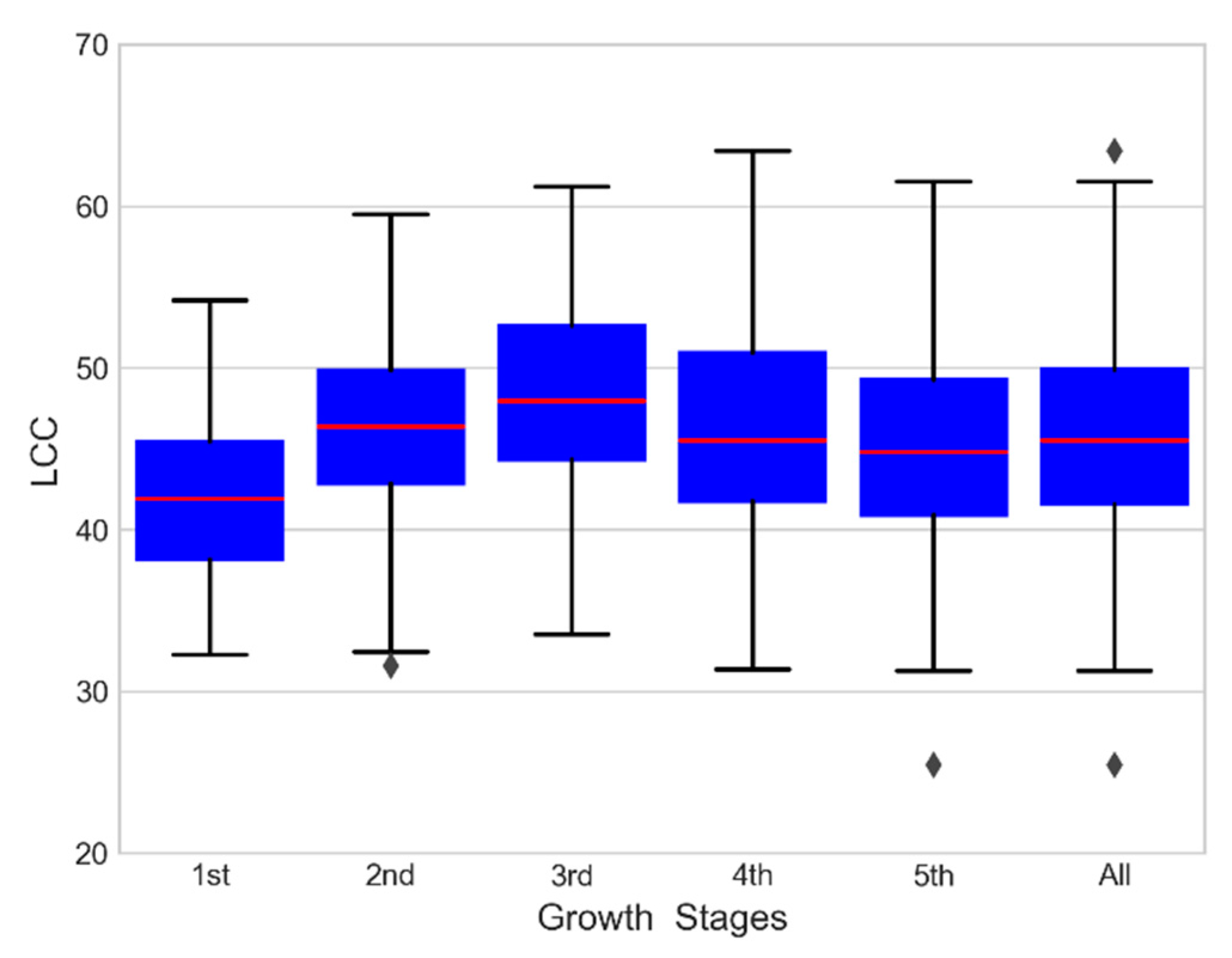
The range of LCC was 25.45 to 63.40, as shown in Table 3. The LCC increased in young expanding leaves, reached the highest value at maturity, and then decreased significantly during senescence. The measured LCC increased gradually from the 1st growth stage to the 3rd growth stage and decreased to a minimum at the 5th growth stage (Figure 2).

Figure 2.
Measured LCC in this study.
3.2. Selection of Sensitivity Parameters
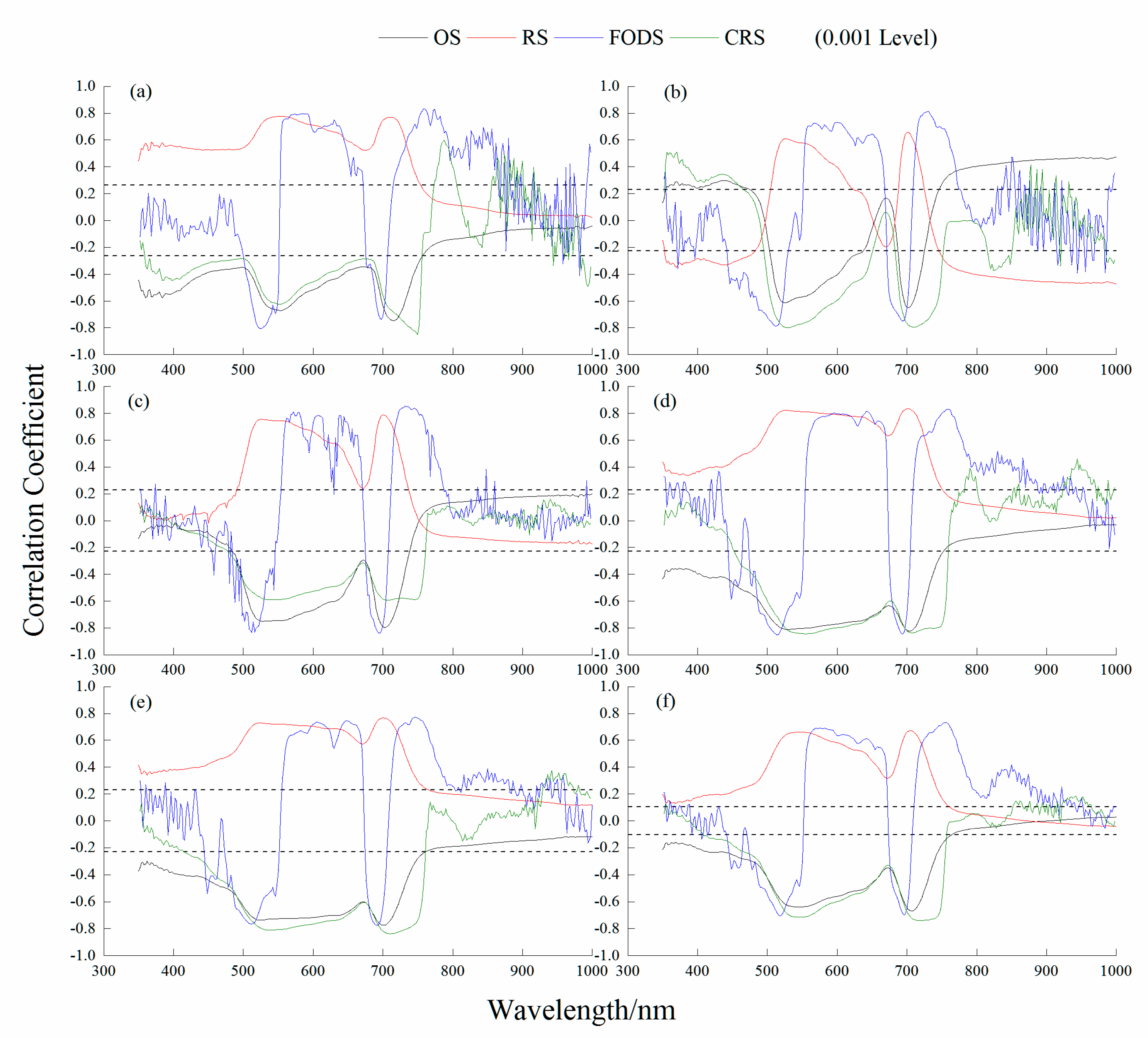
Table 4 shows that the outcomes of the correlation analysis between the four STs and LCC were extremely significant. The CRS had the highest significant correlation with LCC in the 1st and 5th growth stages and all stages together, with values of 0.85, 0.84 and 0.74, respectively. At the 2nd, 3rd and 4th growth stages, FODS had the highest significant correlation with LCC, with correlation coefficients of 0.81, 0.86 and 0.85, respectively. All the sensitive wavebands of STs were selected in the visible band: CRS at 750 nm, FODS at 730 nm, FODS at 732 nm, FODS at 514 nm, CRS at 710 nm, and CRS at 718 nm at the 1st to 5th and All growth stages, respectively (Figure 3).

Table 4.
Correlation relationship between LCC and different variables.
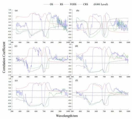
Figure 3.
Correlation coefficients between LCC and spectral transformation at the different growth stages. (a) 1st growth stage; (b) 2nd growth stage; (c) 3rd growth stage; (d) 4th growth stage; (e) 5th growth stage; (f) All growth stages. OS: original spectrum; RS: reciprocal transformed spectrum; FODS: first−order differential spectrum; CRS: continuum removal spectrum.
The relationships between the NDSI and LCC at the 1st growth stage had the highest correlation, with a correlation coefficient of 0.80. Except for the 1st growth stage, the correlation between LCI and LCC was highest at the 2nd, 3rd, 4th, 5th and All growth stages, and the correlation coefficients were 0.79, 0.87, 0.86, 0.84, and 0.75, respectively. As shown in Table 4, SDr/SDb, SDr/SDy, and (SDr − SDb)/(SDr + SDb) had the best correlation with LCC at different growth stages.
3.3. ULR
ULR was performed to identify the three most appropriate and sensitive parameters (ST, VIs, and TEP) for LCC estimation using spectral datasets. The three parameters (ST, VIs, and TEP) were set as the independent variables, LCC was set as the dependent variable, and the optimal fitting models were used. In Table 5, a linear model was established by correlation analysis to obtain the R2 and RMSE of the calibration and validation datasets. The R2 values of the calibration datasets were all greater than 0.60 at every growth stage. A single ST had the best LCC performance at the 1st growth stage, and the R2 and RMSE were 0.75 and 2.44, respectively. A single VI had the best LCC performance at the 3rd growth stage, and the R2 and RMSE were 0.75 and 2.96, respectively. A single TEP had the best LCC performance at the 3rd growth stage, and the R2 and RMSE were 0.74 and 2.98, respectively. All these relationships were significant at p < 0.01.

Table 5.
Regression analysis and curve fitting results of three parameters versus LCC.
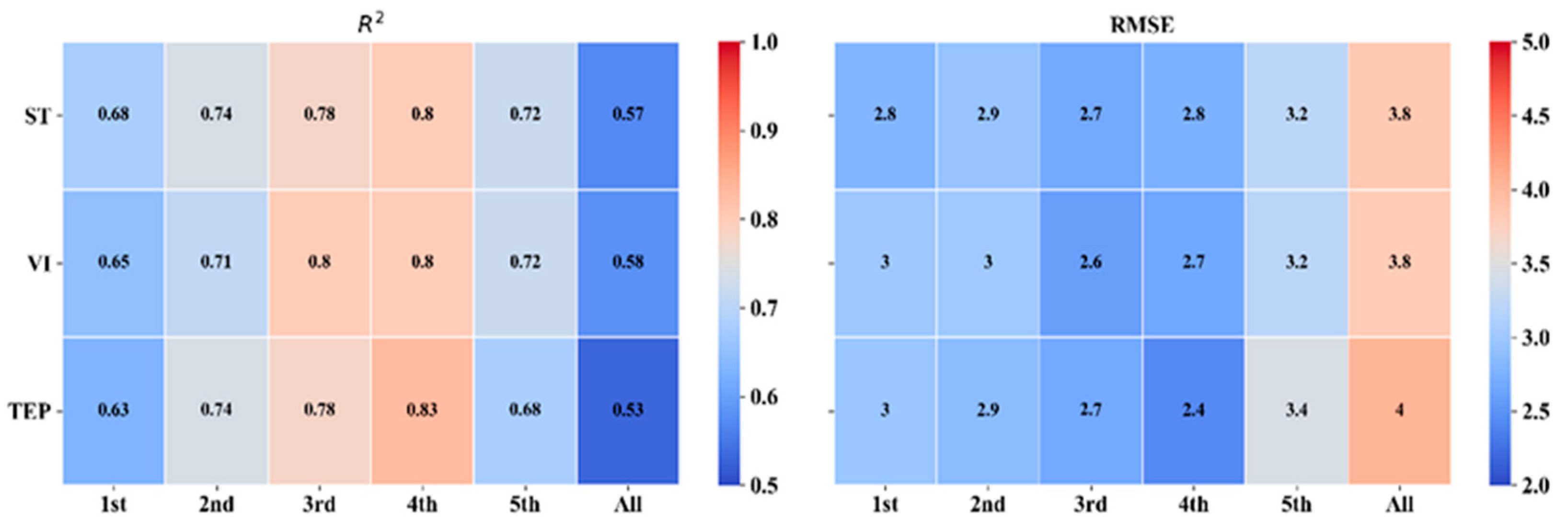
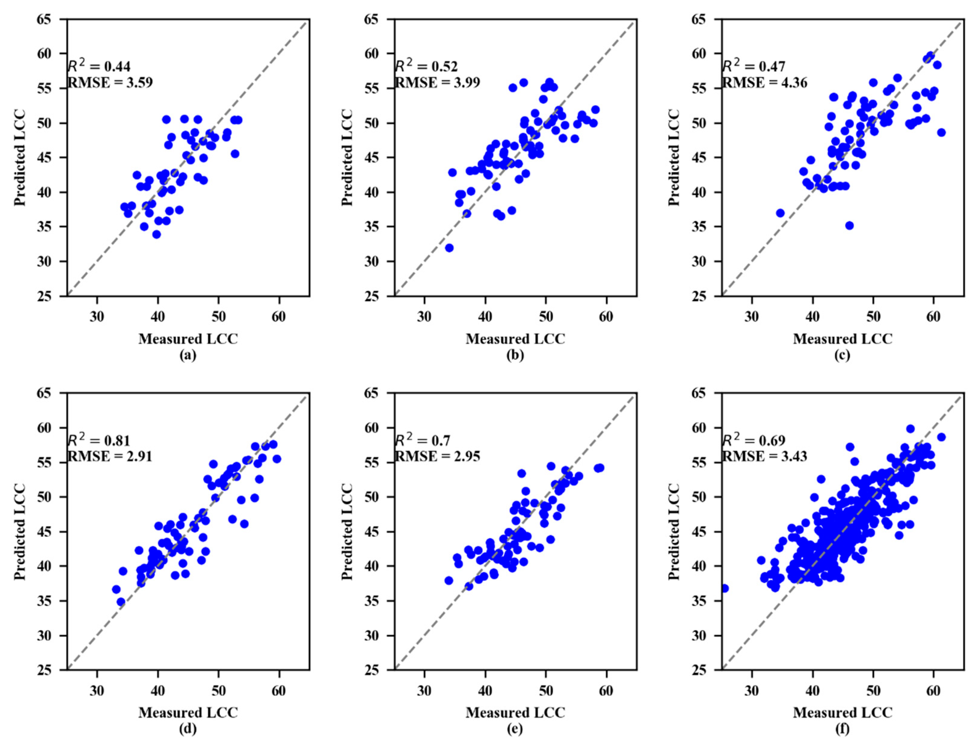
The ST, VIs, and TEP were established by the regression models for the prediction of LCC at different growth stages, which were validated using the validation datasets, and the results are shown in Figure 4. The R2 and RMSE of the validation datasets under different growth conditions and the R2 of the validation datasets were all greater than 0.50.
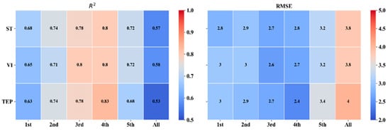
Figure 4.
R2 and RMSE of validation datasets at different growth stages. Spectrum translation (ST), vegetation indices (VIs), and three edge parameters (TEP).
3.4. MLR
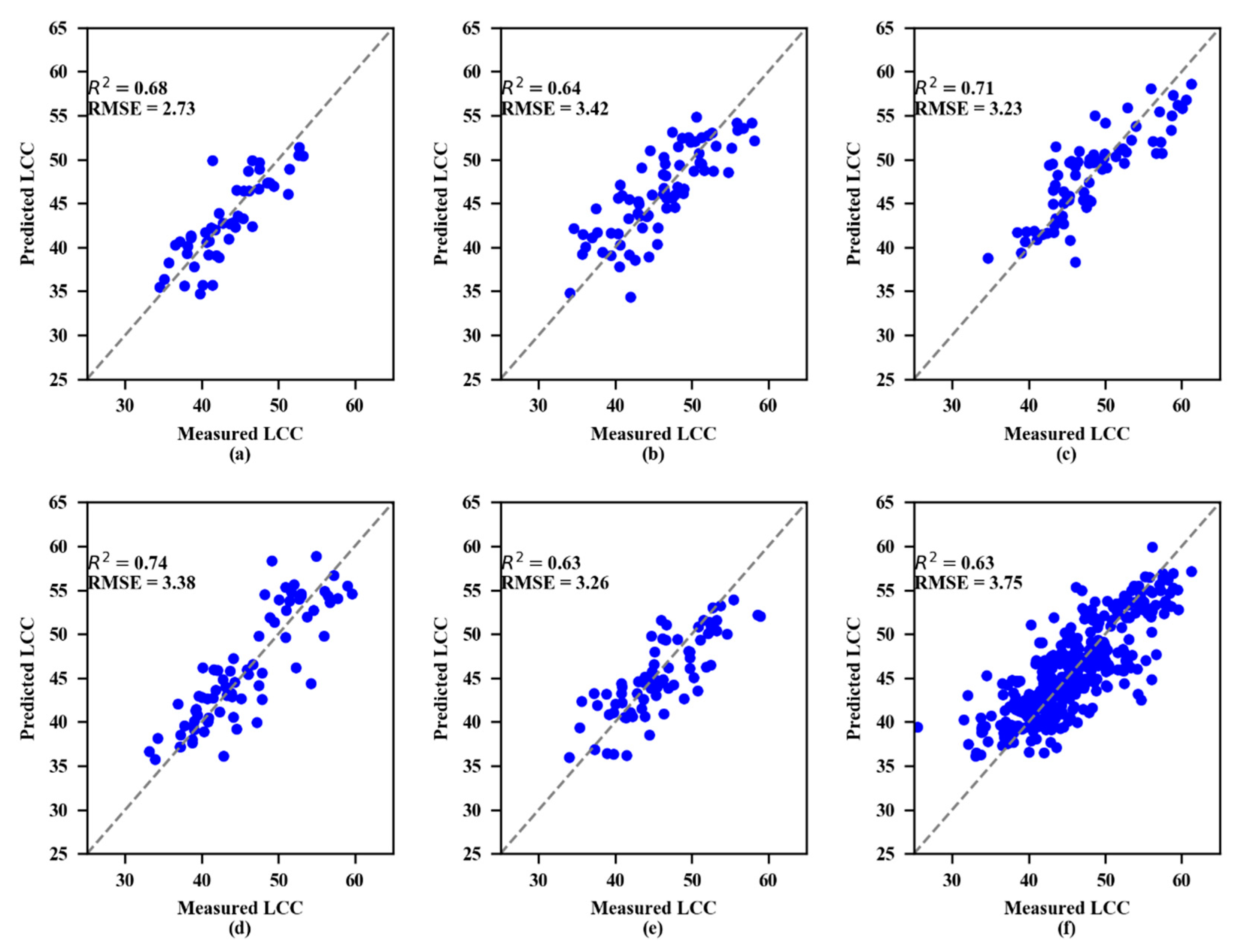
In this section, the three best parameters (ST, VIs, and TEP) were selected and combined to predict the LCC at different growth stages. The MLR analysis results indicated that R2 was 0.66–0.79 and RMSE was 2.27–3.40 (Table 6). The estimation model at the 3rd growth stage had the highest R2 (0.79) and lowest RMSE (2.46) compared with the other growth stages. These MLR models performed better than models based on a single parameter in terms of R2 and RMSE. In addition, the R2 of the validation datasets for each growth stage was greater than 0.60, and the RMSE was low (Figure 5).

Table 6.
Multiple variate linear regression analysis model in calibration datasets.

Figure 5.
Measured and predicted LCC along the 1:1 line in the standalone validation dataset of the MLR models. (a) 1st growth stage, (b) 2nd growth stage, (c) 3rd growth stage, (d) 4th growth stage, (e) 5th growth stage, and (f) All growth stages.
This suggested that multiparameter modeling was feasible at each growth stage. Based on this result, these parameters were used to build a machine learning algorithm model and to reveal the impact of the complex algorithm on LCC inversion in the multivariate case.
3.5. Machine Learning Models
The parameters of the machine learning methods (SVR and RF) were optimized by the grid search method to obtain the best parameters and the calibration dataset coefficients R2 and RMSE, as shown in Table 7. Moreover, the R2 values of RF were higher than SVR for LCC estimation. For RF, the R2 values were all greater than or equal to 0.94. However, for SVR, the R2 values were rarely higher than 0.80, with the highest being approximately 0.82.

Table 7.
R2 and RMSE of calibration datasets in the machine learning models.
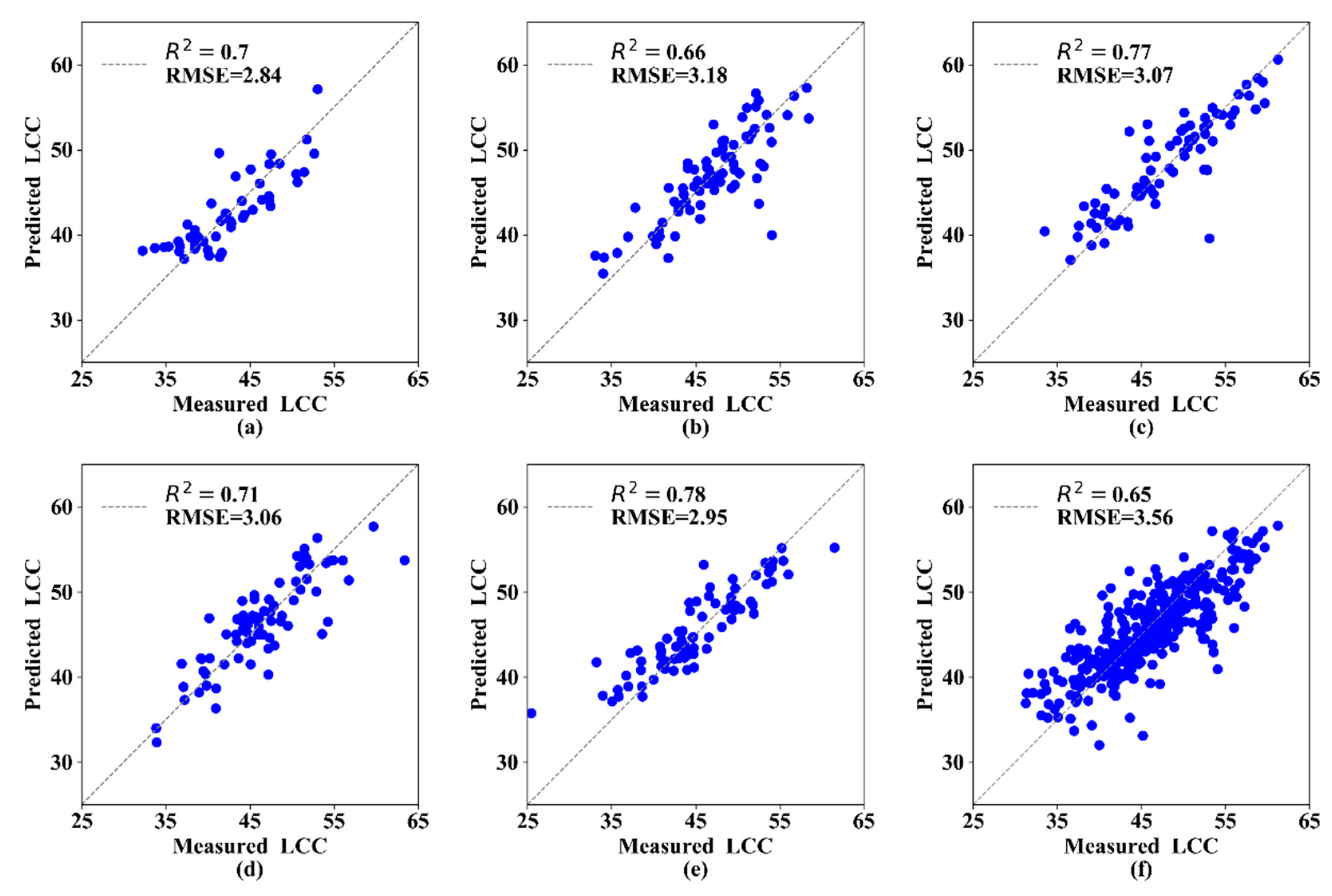
The validation results showed that both the SVR and RF models performed best at the 4th growth stage (Figure 6 and Figure 7, respectively). To estimate LCC, the RF models consistently performed better than the SVR models at every growth stage.
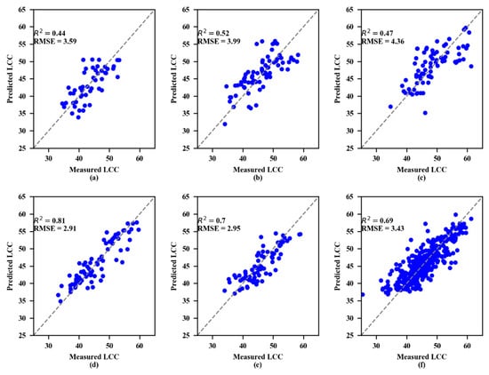
Figure 6.
Measured and predicted LCC along the 1:1 line in the standalone validation datasets of the support vector regression (SVR) model. (a) 1st growth stage, (b) 2nd growth stage, (c) 3rd growth stage, (d) 4th growth stage, (e) 5th growth stage, and (f) All growth stages.

Figure 7.
Measured and predicted LCC along the 1:1 line in the standalone validation datasets of the random forest (RF) model. (a) 1st growth stage, (b) 2nd growth stage, (c) 3rd growth stage, (d) 4th growth stage, (e) 5th growth stage, and (f) All growth stages.
4. Discussion
4.1. Selected Optimized Spectral Indices
Hyperspectral RS is commonly used to monitor seasonal changes in the LCC of crops. In this study, a correlation analysis between three spectral variables (ST, VIs, and TEP) and LCC is shown in Table 4. The results of this study indicate that FODS had the best sensitivity to LCC at the 2nd, 3rd, and 4th growth stages and that CRS had the best sensitivity to LCC at the 1st and 5th growth stages and in All growth stages combined. The most relevant VI of the 1st growth stage was the NDSI, the most relevant VI of other growth stages was the LCI, and the correlation coefficients were all greater than 0.70. In this study, a correlation analysis between TEP and LCC showed that SDr/SDb, SDr/SDy, and (SDr − SDb)/ (SDr + SDb) had the best correlation with LCC; the correlation coefficients were 0.81, 0.81, 0.87, 0.88, 0.82, and 0.73 at the 1st, 2nd, 3rd, 4th, 5th and All growth stages, respectively. These results may be attributed to the reflectance in the red-edge region (680–760 nm) being closely related to the chlorophyll content in apple trees, which has always been considered important in relationships between biochemical or biophysical parameters [44].
In summary, the first-order differential spectrum (FODS) and (SDr − SDb)/(SDr + SDb) are generally the most sensitive to apple leaf chlorophyll content. In previous research, the first derivative was closely related to LCC in wheat crops [45], which was designed to eliminate background signals or noise and to resolve overlapping spectral features. In the future, we will use the spectral data after spectral transformation for models, and spectral transformation could improve the accuracy of the model. The vegetation index has begun to be used more and more in research evaluating crop parameters, but some of the previously researched vegetation indices may not be suitable for future research. Therefore, the vegetation index will be developed or optimized in future research.
4.2. Comparison of Estimation Models with LCC
In this study, LCC was estimated using ST, VIs and TEP alone at different growth stages. The SLR results indicate that ST, VIs and TEP alone best predicted LCC at the 1st, 3rd, and 4th growth stages, and the highest R2 values for these stages were 0.75, 0.75 and 0.74, respectively (Table 5). The MLR regression results indicated that the combination parameter had the best estimated LCC at the 3rd growth stage, at which the R2 value was 0.79 (Table 6). These results demonstrate that using ST, VIs and TEP predicted LCC to have seasonable features. In addition, farmers can perform measurements and use appropriate amounts of fertilizer at the 3rd growth stage. Apple tree leaves had the highest LCC at the 3rd growth stage (Figure 2).
The U/M linear regression models can provide only linear estimations, while ML methods can determine nonlinear relationships. Machine learning (RF and SVR) methods provided better estimations than methods based on linear regression. The machine learning algorithms, especially the RF models, which had the best estimation capacity, all resulted in higher calibration than the U/M linear regression models; however, for the validation datasets, the RF and SVR models performed unevenly at different growth stages. These results could indicate that ML modeling has an overfitting issue [46].
However, multiple variable regression models encompass linear models and machine learning models (SVR and RF) that were used in this study. More research has demonstrated that machine learning models can predict apple tree leaf chlorophyll content [8,47]. The RF regression algorithm is an ensemble-learning algorithm that combines a broad set of regression trees. A regression tree represents a set of conditions or restrictions that are hierarchically organized and successively applied from the roots to the leaves of a tree [48]. The SVM algorithm is based on statistical learning theory and can be regarded as the same type of network, which can also be used for both classification and regression problems [49]. ML models all achieved better results than linear regression models with respect to calibration, but the accuracy of the RF models was lower than that of the SVR models in the validation analysis. A possible reason for such results is that the RF model often results in an overfitting phenomenon, and the robustness and generalization ability of RF are stronger than those of the other SVR methods [46]. Although linear regression models performed slightly worse than ML models in this study, these approaches possessed an extremely fast processing speed; this attribute indicates that these methods comprise a promising technique that can be integrated into crop monitoring systems.
4.3. Challenges and Future Research
In this study, MLR models and machine learning models (SVR and RF) were established using indoor measurement spectral data to assess LCC data at different growth stages. Machine learning methods can improve the prediction accuracy of leaf chlorophyll content at different growth stages. However, this research found that MLR models and machine learning (SVR and RF) models showed decrease sensitivity various at growth stages. In the future, we need to optimize the model to further improve prediction accuracy and stability. In addition, an increasing number of advanced technologies, such as unmanned aerial vehicles (UAVs) and satellite RS images, are now used to retrieve crop growth parameters and physiological parameters [50,51]. We will use these advanced technologies in future research and develop more machine learning methods to evaluate the growth information and physiological parameters of orchard fruit trees and provide technical support for intelligent orchard management.
5. Conclusions
Experiments undertaken using machine learning and statistical regression methods included an analysis of ST, VIs, and TEP. Notably, using the RF algorithm significantly improved the predictability and accuracy of the model in terms of the R2 and RMSE values. Our results also showed that the prediction models of different growth stages were better in their prediction accuracy when using the RF model (R2 = 0.96) and that the prediction accuracy for the 1st growth stage was the best with the RF model. The results indicated that the predicted LCC follows seasonal patterns. Furthermore, evaluating the 1st growing season using the RF model can provide reasonable accuracy for each growth stage.
Author Contributions
Conceptualization: N.T. and Q.C.; methodology: N.T. and Y.Z.; formal analysis: N.T. and Y.Z.; data curation: N.T.; writing—original draft preparation: N.T.; visualization: Y.Z.; project administration: Q.C.; funding acquisition: Q.C. All authors have read and agreed to the published version of the manuscript.
Funding
This work is funded by the Hi-Tech Research and Development Program (863) of China (2013AA102401-2).
Informed Consent Statement
Not applicable.
Data Availability Statement
The experimental data were measured according to the test specifications, which can be used for further analysis.
Conflicts of Interest
The authors declare no conflict of interest.
References
- Gitelson, A.A.; Merzlyak, M.N. Remote estimation of chlorophyll content in higher plant leaves. Int. J. Remote Sens. 1997, 18, 2691–2697. [Google Scholar] [CrossRef]
- Peng, Y.; Nguy-Robertson, A.; Arkebauer, T.; Gitelson, A.A. Assessment of Canopy Chlorophyll Content Retrieval in Maize and Soybean: Implications of Hysteresis on the Development of Generic Algorithms. Remote Sens. 2017, 9, 226. [Google Scholar] [CrossRef] [Green Version]
- Merzlyak, M.N.; Gitelson, A.A.; Chivkunova, O.B.; Rakitin, V.Y. Non-destructive optical detection of pigment changes during leaf senescence and fruit ripening. Physiol. Plant. 1999, 106, 135–141. [Google Scholar] [CrossRef] [Green Version]
- Ustin, S.L.; Valko, P.G.; Kefauver, S.C.; Santos, M.J.; Zimpfer, J.F.; Smith, S.D. Remote sensing of biological soil crust under simulated climate change manipulations in the Mojave Desert. Remote Sens. Environ. 2009, 113, 317–328. [Google Scholar] [CrossRef]
- Gitelson, A.A.; Viña, A.; Ciganda, V.; Rundquist, D.C.; Arkebauer, T.J. Remote estimation of canopy chlorophyll content in crops. Geophys. Res. Lett. 2005, 32, 1–4. [Google Scholar] [CrossRef] [Green Version]
- Upreti, D.; Huang, W.; Kong, W.; Pascucci, S.; Pignatti, S.; Zhou, X.; Ye, H.; Casa, R. A Comparison of Hybrid Machine Learning Algorithms for the Retrieval of Wheat Biophysical Variables from Sentinel-2. Remote Sens. 2019, 11, 481. [Google Scholar] [CrossRef] [Green Version]
- Peuelas, J.; Filella, I. Visible and near-infrared reflectance techniques for diagnosing plant physiological status. Trends Plant Sci. 1998, 3, 151–156. [Google Scholar] [CrossRef]
- Shah, S.H.; Angel, Y.; Houborg, R.; Ali, S.; McCabe, M.F. A Random Forest Machine Learning Approach for the Retrieval of Leaf Chlorophyll Content in Wheat. Remote Sens. 2019, 11, 920. [Google Scholar] [CrossRef] [Green Version]
- Cui, B.; Zhao, Q.; Huang, W.; Song, X.; Ye, H.; Zhou, X. A New Integrated Vegetation Index for the Estimation of Winter Wheat Leaf Chlorophyll Content. Remote Sensor 2019, 11, 974. [Google Scholar] [CrossRef] [Green Version]
- Zhu, W.; Sun, Z.; Yang, T.; Li, J.; Peng, J.; Zhu, K.; Li, S.; Gong, H.; Lyu, Y.; Li, B.; et al. Estimating leaf chlorophyll content of crops via optimal unmanned aerial vehicle hyperspectral data at multi-scales. Comput. Electron. Agric. 2020, 178, 105786. [Google Scholar] [CrossRef]
- Li, C.; Zhu, X.; Wei, Y.; Cao, S.; Guo, X.; Yu, X.; Chang, C. Estimating apple tree canopy chlorophyll content based on Sentinel-2A remote sensing imaging. Sci. Rep. 2018, 8, 1–10. [Google Scholar] [CrossRef] [PubMed]
- Moghimi, A.; Pourreza, A.; Zuniga-Ramirez, G.; Williams, L.; Fidelibus, M. A Novel Machine Learning Approach to Estimate Grapevine Leaf Nitrogen Concentration Using Aerial Multispectral Imagery. Remote Sens. 2020, 12, 3515. [Google Scholar] [CrossRef]
- Wang, L.; Chang, Q.; Li, F.; Yan, L.; Huang, Y.; Wang, Q.; Luo, L. Effects of Growth Stage Development on Paddy Rice Leaf Area Index Prediction Models. Remote Sens. 2019, 11, 361. [Google Scholar] [CrossRef] [Green Version]
- Liang, S.; Zhu, X.C. Hyperspectral estimation models of chlorophyll content in apple leaves. Spectrosc Spect Anal. 2012, 32, 1367–1370. [Google Scholar] [CrossRef]
- Kong, W.; Huang, W.; Casa, R.; Zhou, X.; Ye, H.; Dong, Y. Off-Nadir Hyperspectral Sensing for Estimation of Vertical Profile of Leaf Chlorophyll Content within Wheat Canopies. Sensors 2017, 17, 2711. [Google Scholar] [CrossRef] [Green Version]
- Jin, X.; Li, Z.; Feng, H.; Xu, X.; Yang, G. Newly Combined Spectral Indices to Improve Estimation of Total Leaf Chlorophyll Content in Cotton. IEEE J. Sel. Top. Appl. Earth Obs. Remote Sens. 2014, 7, 4589–4600. [Google Scholar] [CrossRef]
- Jin, X.; Wang, K.-R.; Xiao, C.-H.; Diao, W.-Y.; Wang, F.-Y.; Chen, B.; Li, S.-K. Comparison of two methods for estimation of leaf total chlorophyll content using remote sensing in wheat. Field Crop. Res. 2012, 135, 24–29. [Google Scholar] [CrossRef]
- Zhu, Y.; Yang, G.; Yang, H.; Zhao, F.; Han, S.; Chen, R.; Zhang, C.; Yang, X.; Liu, M.; Cheng, J.; et al. Estimation of Apple Flowering Frost Loss for Fruit Yield Based on Gridded Meteorological and Remote Sensing Data in Luochuan, Shaanxi Province, China. Remote Sens. 2021, 13, 1630. [Google Scholar] [CrossRef]
- Li, F.; Wang, L.; Liu, J.; Wang, Y.; Chang, Q. Evaluation of Leaf N Concentration in Winter Wheat Based on Discrete Wavelet Transform Analysis. Remote Sens. 2019, 11, 1331. [Google Scholar] [CrossRef] [Green Version]
- Costa, C.; Dwyer, L.M.; Dutilleul, P.; Stewart, D.W.; Ma, B.L.; Smith, D.L. Inter-relationships of applied nitrogen, SPAD, and yeild of leafy and non-leafy maize genotypes. J. Plant Nutr. 2001, 24, 1173–1194. [Google Scholar] [CrossRef]
- Huanjun, L.; Wu, B.; Zhao, C.; Zhao, Y. Effect of spectral resoIution on black soil organic matter content predicting model based on laboratory renectance. Spectrosc Spect Anal. 2012, 32. [Google Scholar] [CrossRef]
- Marabel, M.; Alvarez-Taboada, F. Spectroscopic Determination of Aboveground Biomass in Grasslands Using Spectral Transformations, Support Vector Machine and Partial Least Squares Regression. Sensors 2013, 13, 10027–10051. [Google Scholar] [CrossRef] [PubMed] [Green Version]
- Ding, Y.; Li, M.; Zheng, L.; Sun, H. Estimation of tomato leaf nitrogen content using continuum-removal spectroscopy analysis technique. Proc. Spie 2012, 8527, 19. [Google Scholar]
- Rouse, J.W.; Haas, R.H.; Schell, J.A.; Deering, D.W. Monitoring Vegetation Systems in the Great Okains with ERTS. In Proceedings of the 3rd Earth Resources Technology Satellite-1 Symposium, Washington, DC, USA, 10–14 December 1974; pp. 325–333. [Google Scholar]
- Daughtry, C.S.T.; Walthall, C.L.; Kim, M.S.; De Colstoun, E.B.; McMurtrey, J. E Estimating Corn Leaf Chlorophyll Concentration from Leaf and Canopy Reflectance. Remote Sens. Environ. 2000, 74, 229–239. [Google Scholar] [CrossRef]
- Datt, B. A New Reflectance Index for Remote Sensing of Chlorophyll Content in Higher Plants: Tests using Eucalyptus Leaves. J. Plant Physiol. 1999, 154, 30–36. [Google Scholar] [CrossRef]
- Jordan, C.F. Derivation of Leaf-Area Index from Quality of Light on the Forest Floor. Ecology 1969, 50, 663–666. [Google Scholar] [CrossRef]
- Turpie, K.R. Explaining the Spectral Red-Edge Features of Inundated Marsh Vegetation. J. Coast. Res. 2013, 290, 1111–1117. [Google Scholar] [CrossRef]
- Gitelson, A.A.; Kaufman, Y.J.; Merzlyak, M.N. Use of a green channel in remote sensing of global vegetation from EOS-MODIS. Remote Sens. Environ. 1996, 58, 289–298. [Google Scholar] [CrossRef]
- Gamon, J.A.; Peñuelas, J.; Field, C.B. A narrow-waveband spectral index that tracks diurnal changes in photosynthetic efficiency. Remote Sens. Environ. 1992, 41, 35–44. [Google Scholar] [CrossRef]
- Blackburn, G.A. Spectral indices for estimating photosynthetic pigment concentrations: A test using senescent tree leaves. Int. J. Remote Sens. 1998, 19, 657–675. [Google Scholar] [CrossRef]
- Metternicht, G. Vegetation indices derived from high-resolution airborne videography for precision crop management. Int. J. Remote Sens. 2003, 24, 2855–2877. [Google Scholar] [CrossRef]
- Penuelas, J.; Baret, F.; Filella, I. Semi-empirical indices to assess carotenoids / chlorophyll a ratio from leafspectral reflectance. Photosynthetica 1995, 31, 221–230. [Google Scholar]
- Inoue, Y.; Penuelas, J.; Miyata, A.; Mano, M. Normalized difference spectral indices for estimating photosynthetic efficiency and capacity at a canopy scale derived from hyperspectral and CO2 flux measurements in rice. Remote Sens. Environ. 2008, 112, 156–172. [Google Scholar] [CrossRef]
- Li, X.-Y.; Liu, G.-S.; Yang, Y.-F.; Zhao, C.-H.; Yu, Q.-W.; Song, S.-X. Relationship Between Hyperspectral Parameters and Physiological and Biochemical Indexes of Flue-Cured Tobacco Leaves. Agric. Sci. China 2007, 6, 665–672. [Google Scholar] [CrossRef]
- Noi, P.T.; Degener, J.; Kappas, M. Comparison of Multiple Linear Regression, Cubist Regression, and Random Forest Algorithms to Estimate Daily Air Surface Temperature from Dynamic Combinations of MODIS LST Data. Remote Sens. 2017, 9, 398. [Google Scholar] [CrossRef] [Green Version]
- Clevers, J.G.P.W.; Kooistra, L.; Brande, M.M.M.V.D. Using Sentinel-2 Data for Retrieving LAI and Leaf and Canopy Chlorophyll Content of a Potato Crop. Remote Sens. 2017, 9, 405. [Google Scholar] [CrossRef] [Green Version]
- Cheng, T.; Song, R.; Li, D.; Zhou, K.; Zheng, H.; Yao, X.; Tian, Y.; Cao, W.; Zhu, Y. Spectroscopic Estimation of Biomass in Canopy Components of Paddy Rice Using Dry Matter and Chlorophyll Indices. Remote Sens. 2017, 9, 319. [Google Scholar] [CrossRef] [Green Version]
- Fu, X.; Mo, W.-P.; Zhang, J.-Y.; Zhou, L.-Y.; Wang, H.-C.; Huang, X.-M. Shoot growth pattern and quantifying flush maturity with SPAD value in litchi (Litchi chinensis Sonn.). Sci. Hortic. 2014, 174, 29–35. [Google Scholar] [CrossRef]
- Breiman, L. Random Forests. Mach. Learn. 2001, 5, 5–32. [Google Scholar] [CrossRef] [Green Version]
- Smola, A.J.; Olkopf, B.S. A tutorial on support vector regression. Stat. Comput. 2004, 14, 199–222. [Google Scholar] [CrossRef] [Green Version]
- Abraham, A.; Pedregosa, F.; Eickenberg, M.; Gervais, P.; Mueller, A.; Kossaifi, J.; Gramfort, A.; Thirion, B.; Varoquaux, G. Machine learning for neuroimaging with scikit-learn. Front. Aging Neurosci. 2014, 8, 14. [Google Scholar] [CrossRef] [Green Version]
- Pedregosa, F.; Varoquax, G.; Gramfort, A.; Michel, V.; Thirion, B.; Grisel, O.; Blondel, M.; Prettenhofer, P.; Weiss, R.; Dubourg, V.; et al. Scikit-learn machine learning in python. J. Mach. Learn. Res. 2011, 12, 2825–2830. [Google Scholar]
- Cho, M.A.; Skidmore, A.K. A new technique for extracting the red edge position from hyperspectral data: The linear extrapolation method. Remote Sens. Environ. 2006, 101, 181–193. [Google Scholar] [CrossRef]
- Ju, C.-H.; Tian, Y.-C.; Yao, X.; Cao, W.-X.; Zhu, Y.; Hannaway, D. Estimating Leaf Chlorophyll Content Using Red Edge Parameters. Pedosphere 2010, 20, 633–644. [Google Scholar] [CrossRef]
- Zheng, H.; Li, W.; Jiang, J.; Liu, Y.; Cheng, T.; Tian, Y.; Zhu, Y.; Cao, W.; Zhang, Y.; Yao, X. A Comparative Assessment of Different Modeling Algorithms for Estimating Leaf Nitrogen Content in Winter Wheat Using Multispectral Images from an Unmanned Aerial Vehicle. Remote Sens. 2018, 10, 2026. [Google Scholar] [CrossRef] [Green Version]
- Dutta, D.; Das, P.K.; Bhunia, U.K.; Singh, U.; Singh, S.; Sharma, J.R.; Dadhwal, V.K. Retrieval of tea polyphenol at leaf level using spectral transformation and multi-variate statistical approach. Int. J. Appl. Earth Obs. Geoinf. 2014, 36, 22–29. [Google Scholar] [CrossRef]
- Li’ai, W.; Zhou, X.; Zhu, X.; Dong, Z.; Guo, W. Estimation of biomass in wheat using random forest regression algorithm and remote sensing data. Crop. J. 2016, 3, 62–69. [Google Scholar]
- Durbha, S.S.; King, R.L.; Younan, N.H. Support vector machines regression for retrieval of leaf area index from multiangle imaging spectroradiometer. Remote Sens. Environ. 2007, 107, 348–361. [Google Scholar] [CrossRef]
- Maimaitijiang, M.; Sagan, V.; Sidike, P.; Daloye, A.M.; Erkbol, H.; Fritschi, F.B. Crop Monitoring Using Satellite/UAV Data Fusion and Machine Learning. Remote Sens. 2020, 12, 1357. [Google Scholar] [CrossRef]
- Ali, A.M.; Darvishzadeh, R.; Skidmore, A.; Gara, T.W.; O’Connor, B.; Roeoesli, C.; Heurich, M.; Paganini, M. Comparing methods for mapping canopy chlorophyll content in a mixed mountain forest using Sentinel-2 data. Int. J. Appl. Earth Obs. Geoinf. 2020, 87, 102037. [Google Scholar] [CrossRef]
Publisher’s Note: MDPI stays neutral with regard to jurisdictional claims in published maps and institutional affiliations. |
© 2021 by the authors. Licensee MDPI, Basel, Switzerland. This article is an open access article distributed under the terms and conditions of the Creative Commons Attribution (CC BY) license (https://creativecommons.org/licenses/by/4.0/).

