Abstract
Automatically extracting buildings from remote sensing images with deep learning is of great significance to urban planning, disaster prevention, change detection, and other applications. Various deep learning models have been proposed to extract building information, showing both strengths and weaknesses in capturing the complex spectral and spatial characteristics of buildings in remote sensing images. To integrate the strengths of individual models and obtain fine-scale spatial and spectral building information, this study proposed a stacking ensemble deep learning model. First, an optimization method for the prediction results of the basic model is proposed based on fully connected conditional random fields (CRFs). On this basis, a stacking ensemble model (SENet) based on a sparse autoencoder integrating U-NET, SegNet, and FCN-8s models is proposed to combine the features of the optimized basic model prediction results. Utilizing several cities in Hebei Province, China as a case study, a building dataset containing attribute labels is established to assess the performance of the proposed model. The proposed SENet is compared with three individual models (U-NET, SegNet and FCN-8s), and the results show that the accuracy of SENet is 0.954, approximately 6.7%, 6.1%, and 9.8% higher than U-NET, SegNet, and FCN-8s models, respectively. The identification of building features, including colors, sizes, shapes, and shadows, is also evaluated, showing that the accuracy, recall, F1 score, and intersection over union (IoU) of the SENet model are higher than those of the three individual models. This suggests that the proposed ensemble model can effectively depict the different features of buildings and provides an alternative approach to building extraction with higher accuracy.
1. Introduction
Automatic extraction of buildings from remote sensing imagery is of great significance for many applications, such as urban planning, environmental research, change detection and digital city construction [1,2,3]. Recently, substantial improvements in the capabilities of remote sensing techniques have been achieved and have led to a dramatic increase in the availability and accessibility of high-resolution remote sensing images [4]. The high spatial resolution of remote sensing imagery reveals fine details in urban areas and greatly facilitates automatic building extraction. However, the diverse characteristics of buildings, including color, shape, size, and the interference of building shadows [5], make the development of an accurate and reliable building extraction method a challenging task.
Over the past few decades, various approaches for feature extraction from images have been developed. Spatial and textural features of images are extracted through mathematical descriptors, such as the scale-invariant feature transform (SIFT) [6], local binary patterns (LBPs) [7], and histograms of oriented gradients (HOGs) [8]. More recently, pixel-by-pixel predictions were introduced based on extracted features through classifiers, such as support vector machines (SVMs) [9], adaptive boosting (AdaBoost) [10], random forests [11], and conditional random fields (CRFs) [12]. However, these methods rely heavily on manual feature designs and implementations, which generally change with the application area. As a consequence, they can easily introduce biases, have poor generalization abilities, and are time-consuming and labor-intensive.
With the rapid development of computer technology, deep learning methods have shown strong performance in classification and detection in the field of image processing. In the past decade, convolutional neural network (CNN) models, such as fully convolutional networks (FCNs) [13], SegNet [14], U-Net [15], and LinkNet [16], have been proposed by researchers and have been widely used for extracting buildings from remote sensing images. Mnih [17] and Saito et al. [18] transformed the output of a fully connected layer of a CNN into the predicted block to achieve building extraction. Bittner et al. [19] implemented an FCN that effectively combined high-resolution images with normalized DSMs and automatically generated architectural predictions. Based on these classical semantic segmentation models, research has optimized and proposed improved models suitable for building extraction. Yi et al. [20] compared the building extraction performance of the proposed DeepResUNet with other semantic segmentation architectures: FCN-8s, SegNet, DeconvNet [21], U-Net, ResUNet [22], and DeepUNet [23]. Pan et al. [24] used a generative adversarial network model with spatial and channel attention mechanisms to select more useful features for building extraction and compared their method with the classical model to verify the superiority of different methods. Ye et al. [25] proposed a novel FCN that adopts attention-based reweighting to extract buildings from aerial imagery. The advantages of the proposed RFA-UNET were verified by comparing it with U-Net, SegNet, RefineNet [26], FC-DenseNet [27], DeepLab-V3Plus [28], and MFRN [29] on three public aerial image datasets. These deep learning models have made great contributions to improving the accuracy of building extraction from remote sensing images.
Despite the strengths of the proposed deep learning models, limitations still exist in extracting building information. Liu et al. [30] found through comparative experiments that U-Net failed to detect holes when extracting large buildings, but it is better than SegNet at recognizing shadows. Zhang et al. [31] found that SegNet often misclassifies shadowed building pixels as nonbuildings. On the other hand, Ma et al. [32] discovered that FCNs and SegNet have smooth boundary predictions and perform better on small buildings compared with other models. In addition, clouds and fog in remote sensing images will also affect the accuracy of model extraction, but there have been many defogging technologies, such as IDE [33] and IDGCP [34], that can effectively solve this problem. Considering the complex characteristics of building shape, structure, color, texture, and other features, it is difficult for an individual deep learning model to maintain high forecasting accuracy and robustness.
Considering the limitations of individual models, research has adopted ensemble learning to combine the advantages of different models. Ensemble learning uses several different individual models and certain ensemble strategies to improve the generalization performance of the entire model and has been proven to be an effective method for overcoming the abovementioned problems [35]. The integration strategies of ensemble learning include averaging, voting, and learning [36,37]. Sun et al. [38] used simple majority voting based on rule images for decision fusion to refine boundaries and reduce noise. Saqlain et al. [39] proposed a voting ensemble classifier with multitype features to identify wafer map defect patterns in semiconductor manufacturing. However, averaging and voting represent the fusion of results at the decision level, which will lead to large learning errors [40]. The learning method represented by stacking can correct errors in the base model to improve the performance of the integrated model and maximize the advantages of different models to a certain extent [32]. Stacking is an ensemble method with a two-layer structure that combines the outputs of more than two base models via a new (meta) model to find the optimal regression performance. When a stacking technique is used to integrate the features of the output results of the base model, result fusion at the feature level can be achieved.
Motivated by the analysis above, in this study, a deep learning feature integration method based on a stacking ensemble technique is proposed for extracting buildings from remote sensing images. Taking the integration of three CNN models (U-net, SegNet, and FCN-8s) as an example, an ensemble model called SENet was developed. To verify that the model can effectively integrate the advantages of different base models to extract different building features, a dataset was also created for building detection, and feature attribute tags were added to the buildings in the test set. The main contributions of this study are summarized as follows:
- (1)
- A deep learning feature integration method is proposed for extracting buildings from remote sensing images. The method combines the advantages of deep learning and ensemble learning. It can enhance the generalization and robustness of the whole model by integrating the advantages of different CNN models.
- (2)
- An optimization method for the prediction results of the basic model is proposed based on fully connected CRFs. The influence of the number of inference function calculations in the CRFs on the optimization result is analyzed, and the number of inference function calculations needed to obtain the best optimization result is determined.
- (3)
- A stacking ensemble method based on a sparse autoencoder [41] is proposed to combine the features of the optimized basic model prediction results. A sparse autoencoder is used to extract the features of the optimized base model prediction results, and then these features are integrated based on the stacking ensemble technique.
A building dataset is created, and the proposed SENet is compared with three individual models on this dataset. By adding attribute labels to each building sample in the test set, the accuracy of extracting different building features from the model is quantitatively analyzed. The experimental results showed that SENET can effectively integrate different model features and improve the accuracy of building extraction.
The rest of this article is organized as follows. In Section 2, an overview of the method and a description of the dataset are introduced. Section 3 provides descriptions of the experimental results and comparisons of three individual models. Discussions and conclusions are given in Section 4 and Section 5, respectively.
2. Methodology
2.1. Overview of the Proposed Model
The framework of the proposed ensemble deep learning model for building extraction (denoted as SENet) is presented in Figure 1. The overview of the framework consists of three stages: data preparation, basic model construction, and basic model combination. In the data preparation stage, a building dataset from satellite images was created, and the accuracy of the building features extracted by the model was quantitatively analyzed by adding attribute tags to the buildings in the test set. In the basic model construction stage, three CNN models of U-net, SegNet, and FCN-8s are used to train the model and extract features from the building dataset. Furthermore, a method for optimizing the prediction results of the basic model is proposed based on CRFs. In the basic model combination stage, an ensemble method based on a sparse autoencoder is proposed. First, the sparse autoencoder is used to extract the features of the optimized base model prediction results, and then the stacking ensemble technique is used to integrate the features in a weighted way to obtain the final prediction results. In the following subsections, the methods involved in the construction and combination of the basic predictors are described in detail. The data preparation stage will be introduced in Section 3.1.
Figure 1.
Overview of the framework.
2.2. Basic Model Construction
The basic model construction stage consists of two parts, namely to train the basic semantic segmentation models for building extraction and to optimize basic prediction results by using fully connected CRFs.
2.2.1. Semantic Segmentation Models for Building Extraction
Based on the performance of individual models, three representative models, including FCN-8s, U-Net, and SegNet, were selected. Detailed comparisons of the selected models are summarized in Table 1.

Table 1.
Detailed comparisons of FCN-8s, U-Net and SegNet. ’LRP’ denotes the learning rate policy.
The introduction of FCNs has caused a rapid increase in the number of semantic segmentation networks. The FCN model transforms all of the fully connected layers to convolutional layers and allows the input image to be arbitrarily sized. In addition, it combines semantic image information from deep layers with the information from shallow layers to produce the final segmentation result by using a skip architecture. Long et al. [13] proposed three end-to-end FCN models (i.e., FCN-32s, FCN-16s, and FCN-8s), among which FCN-8s was considered the best. Therefore, the FCN-8s model is selected in this study.
U-Net was built upon an FCN and adopts an encoder-decoder architecture that consists of a contracting path to capture context and a symmetric expanding path to enable accurate localization. It was originally designed to segment medical images and achieves good results with fewer training sets. In recent years, some studies have shown that U-Net is also suitable for remote sensing images [42], and it has great potential to be improved.
Similar to U-Net, SegNet is also built on an encoder-decoder structure. Its encoder network is topologically the same as the 13 convolutional layers of VGG-16 [43]. The decoder network first uses max-pooling indexes generated from the corresponding encoder to enhance the location information. Bischke et al. [44] used SegNet with a new cascaded multitask loss to further preserve semantic segmentation boundaries in high-resolution satellite images.
2.2.2. Optimized Basic Prediction Results
The extraction performances of the individual basic models influence the extraction performance of the ultimate ensemble model. It is therefore necessary to optimize the prediction results of a single model before model combination. In this study, fully connected CRFs [45] are introduced to perform postprocessing on the prediction results of the basic model. By combining the relationships among all pixels, the CRF model carries out full connection modeling between adjacent pixels, introduces pixel color information as a reference, and calculates the pixel classification probability according to the prediction results of the basic model [46]. The probability distribution map is calculated as unary potential energy. Thus, each pixel is classified and evaluated, and the classification probability is calculated. Moreover, the position information and color information provided by the input of the original image are used as binary potential energy, and the category energy of the prediction class is finally reduced to the minimum value to achieve the final optimization result. The optimization process is shown in Figure 1(c-1). The input of this process is the prediction result of the basic model, and the output is the prediction result optimized by CRFs.
The energy function of CRFs consists of two parts:
where a is the label assignment for each pixel and is the total number of pixels in the image. is a unary potential energy function, which is mainly used to calculate the probability that a pixel of the input image belongs to category , which can be directly obtained from the CNN. It can predict the label of the pixel without considering the smoothness and consistency of the label assignment. is the binary potential energy function of the energy function, which is mainly used to calculate the mutual influence between pixels and assigns similar labels to similar pixels. The pairwise potential is defined as
where and are the feature vectors of pixels and , respectively, in a feature space, and they are derived from the spatial position and RGB value in the image feature. Each is a Gaussian kernel weighted by . is a label compatibility function, which depends on only the labels and .
To achieve segmentation and labeling of multiple types of images, CRFs use two contrasting Gaussian kernel functions [47,48]. The first kernel function uses the position information and color information of pixels. and are used to represent the positions of pixels and , respectively. and represent the original color values of pixels y and z, respectively; and learnable parameters and are used to determine the spatial proximity and color similarity, respectively. The second kernel uses only pixel position information to remove isolated regions.
where , , , , and are all parameters that can be learned from the model.
2.3. Basic Model Combination
A Stacking Ensemble Method Based on a Sparse Autoencoder
Stacking is an ensemble method with a two-layer structure that combines outputs of more than two base models via a new (meta) model to find the optimal regression performance. This method can correct errors in the basic model to improve the performance of the integrated model and maximize the advantages of different models to a certain extent. The development of computer technology can provide opportunities for deeper networks, but even without increases in depth, network performance has been increasing. Inspired by the designs of the VGG and GoogLeNet [49] structures, the features of different CNN outputs can be used to perform integrated optimization and explore better classification methods. Therefore, a stacking ensemble method based on a sparse autoencoder is proposed in this study. First, the features of the output results of multiple base models optimized by CRFs were selected, and the weight parameters of the primary encoder were obtained by encoding the multilayer features through the sparse autoencoder. Then, the sparse autoencoder is used again to fit the output of the primary encoder with the real output, and the weight parameters of the secondary encoder are obtained. Finally, the output of each subencoder is integrated via Euclidean distance weighting to obtain the final prediction result. As shown in Figure 1(c-2), the input of the sparse autoencoder is the optimized prediction result image, and the output is the feature weight parameter of each image. Figure 1(c-3) shows the process of integrating features based on stacking technology. The input of this process is all the features extracted by the sparse autoencoder, and the output is the final prediction result.
First, it is assumed that the training sample input by the network is , and the feature extracted by the base model is denoted as . According to the idea of a stacking ensemble, the sparse autoencoder is used to construct the first group of learners , which is called the primary encoder. The optimization function of the primary encoder is:
where is the objective function to be optimized, is the true label, is the feature of the input primary encoder, is the parameter matrix of the primary encoder, and is the regularization coefficient. The primary encoder trained by the base model is selected as . Then, the predicted output is . This optimization process shortens the training time. The prediction result after feature passes through the primary encoder is reoptimized and expressed as:
where is the weight matrix of the prediction result of the primary encoder and the expected output and is called the secondary encoder.
The optimized primary encoder parameter and the secondary encoder parameter are obtained by the above method. After inputting the test samples, the predicted output of the secondary encoder is obtained:
The prediction results of each secondary encoder are weighted according to the Euclidean distance between the prediction result and the real label after the feature extracted by each base model passes through the secondary encoder. The larger the distance between the predicted result and the real label is, the smaller the assigned weight. Then, the final predicted result is obtained:
where is the final prediction result and is the weighting coefficient.
3. Experiments and Results
In this section, we first describe the dataset used in the experiments and experimental setting. We then provide qualitative and quantitative comparisons of performances between SENet and other individual models in semantic segmentation of buildings from the same data source.
3.1. Dataset
Based on the proposed model, a building dataset is established to quantitatively evaluate the accuracy of extracting different building features. Currently, publicly available building datasets only provide satellite or aerial images and the corresponding building label data and lack descriptions of the feature attributes of each building sample. Therefore, it is difficult to classify buildings according to their features and calculate the extraction accuracy of each feature after using a deep learning model to extract buildings. Related studies have found that the shape, color, size, texture, and shadow of a building will affect the extraction accuracy of CNN models [30,32,50]. However, the types of texture features are complex and difficult to classify. To solve this issue, the building-feature attribute label including four kinds of feature information, namely, the color, size, shape, and shadow are involved in this study. We counted the number of each roof color in the building dataset and found that the four most common colors were red, blue, white, and gray, so we divided the building color attributes into five categories: red, blue, white, gray, and others. Castagno and Atkins [51] divided building shapes into eight types, unknown, complex flat, flat, gabled, half hipped, hipped, pyramid, and skill (shed), in the study of roof shape classification in lidar images using supervised learning. In this study, the classification results are simplified to describe the shape of buildings in terms of the structure and edge contours. For the size definition, we refer to the size classification standard of buildings in the cost–benefit analysis of green buildings by Gabay et al. [52]. The detailed definitions and descriptions of the building-feature attribute labels are listed in Table 2.
Table 2.
Definitions and descriptions of the building-feature attribute label.
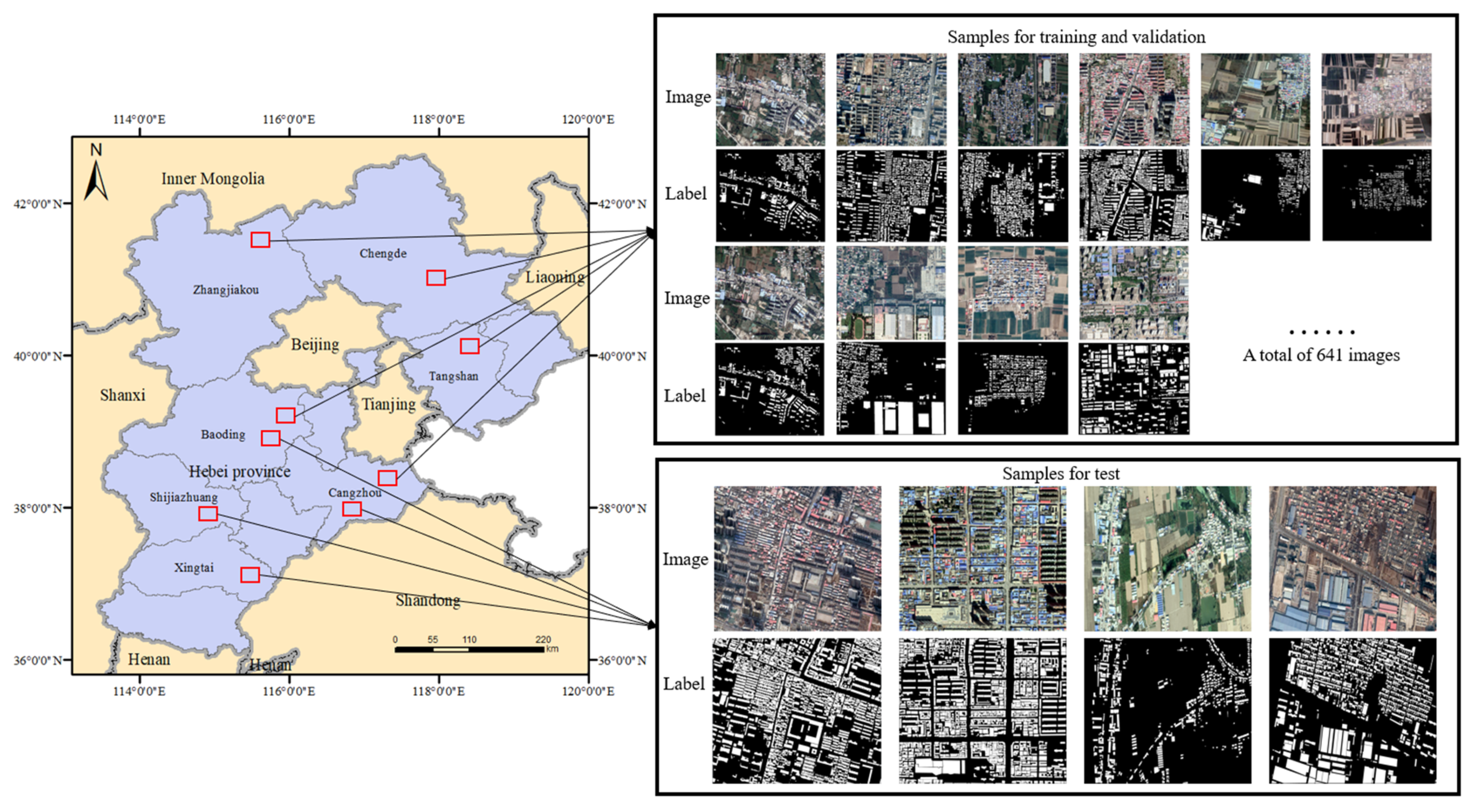
According to the above building-feature attribute labels, we manually created a large-scale satellite image building dataset. As shown in Figure 2, the study area selected for creating the dataset was in several cities, Hebei Province, China and contained 1,029,000 buildings of various types with ground resolutions of 0.27 m. We seamlessly cropped the images according to the subregions of cities, towns, and rural areas and cut out a total of 650 images that were approximately 5000 × 3500 pixels. Then, we drew building vector diagrams and added feature attribute tags in ArcGIS software, stored them in shape file format, and converted them to raster annotation data, as required for deep learning model training.

Figure 2.
Study area and samples for training, validation and testing.
Several high-resolution remote sensing image data were utilized, including QuickBird and Worldview series data, with ground resolutions of up to 0.27 m and three spectral bands (RGB). Since deep learning is a data-driven algorithm, the larger the amount of data is and the more types of data there are, the easier it is for the model to learn representative features. The dataset we created includes a variety of civil, industrial, and agricultural buildings. The building samples include different colors, sizes, shapes, and textures. Figure 3 shows examples of different types of buildings.
Figure 3.
Examples of buildings with different colors, sizes, shapes and textures from the satellite dataset.
3.2. Experimental Setting
The building dataset created in this paper is used as the experimental dataset and contains 650 remote sensing images with 5000 × 3500 pixels and the corresponding building labels. Hence, 10% of the images from the 650 images were selected as the test images. Considering the limitation of video memory size, we cropped all the images with a sliding window of 256 ×256 pixels and divided the remaining 90% of images (from 650 images) into training sets and validation sets. In the training process, the rectified linear unit (ReLU) function is used as the activation function. Instead of the simple mean square error (MSE), binary cross entropy is chosen to calculate the loss between every prediction and relative ground truth. The experiment was conducted with the Keras framework (https://keras.io/, accessed on 29 August 2021) with a TensorFlow GPU (https://tensorflow.google.cn, accessed on 29 August 2021) as the backend, and the Adam algorithm was used for network optimization. All the experiments were carried out on an NVIDIA GeForce RTX 2060 GPU with 64 GB of memory under CUDA 9.0. PyCharm software was employed for developing the suggested algorithm. The proposed SENet and three individual CNN models (U-Net, SegNet, and FCN-8s) were trained and used for prediction on the same dataset. The experiments were carried out in exactly the same experimental environments. Each network was trained from scratch without a pretrained model. The building attribute labels in the test set were used to classify the extracted results according to different attribute features, and the overall extraction accuracy and the fusion of different building features were compared and analyzed.
3.3. Model Performance
3.3.1. Overall Performance
Figure 4 shows the prediction results of four satellite images from the test dataset after training with four models. The first column in the figure shows the buildings in a village. The buildings are small in size and relatively scattered. The prediction results of the SENet and U-Net networks in this region are highly accurate, while some misclassifications (false positives) appeared in the segmentation results of SegNet and FCN-8s. SegNet misclassifies parts of cultivated land as buildings, while FCN-8s misclassifies parts of roads as buildings. The test area in the second column of the figure is a town, and the buildings include compactly arranged small houses and large factories. As seen from the prediction diagram, the extraction accuracies of SENet and FCN-8s are relatively high. Although FCN-8s misclassifies parts of the land into buildings, there are few cases of false negatives (blue). However, the extraction accuracies of U-Net and SegNet in this area are relatively low, both of which have false negatives (blue), and U-Net also has many false positives (red). The third and fourth columns contain images of buildings in a city. The differences between the images in the columns are that the original image in the third column is dark in color, the satellite image was taken at a large tilt angle, and the buildings appear in an irregular arrangement. The images in the fourth column are brightly colored, and the buildings are arranged normally. It can be seen from the figure that the building extraction effect of the four models in the fourth column image is better than that in the third column image. In the third column, U-Net and SegNet appear to have more false negatives (blue), and FCN-8s misclassifies some squares as buildings. In the fourth column, the extraction accuracies of SENet, SegNet, and FCN-8s are very high, and only the U-Net results contain many false negatives (green).
Figure 4.
Segmentation results of the different methods on the test dataset. (a) Original input image. (b) Label map (ground truth). (c) The output of SENet. (d) The output of U-Net. (e) The output of SegNet. (f) The output of FCN-8s. The green, red, and blue pixels of the maps represent true positive, false positive and false negative predictions, respectively.
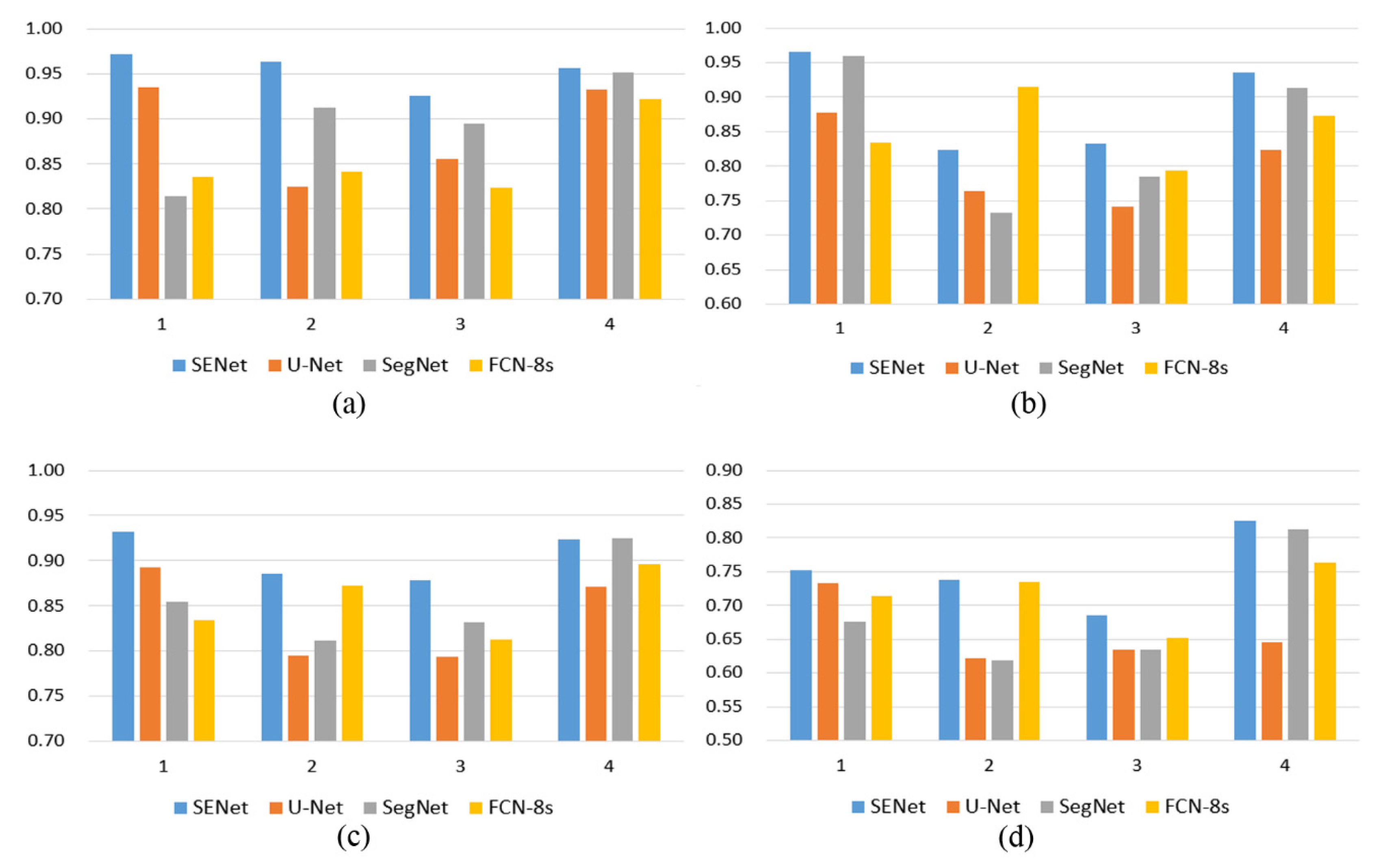
Table 3 and Figure 5 show that the SENet model is better than the other three models in terms of the average of the four evaluation indicators for the four test areas. The U-Net model has the lowest recall rates for the four test areas, which is caused by the excessive number of false negatives (blue) in the predicted results. In terms of precision, FCN-8s has the lowest average value. Figure 4 shows that the FCN-8s model makes more misclassifications (false positives) in the four predicted images, but the FCN-8s has higher recall rates, especially in the second column test images, and fewer false negatives (blue) than the other two individual models. The accuracy, recall, F1 score, and IoU of the experimental results of the SENet model on the test dataset reached 0.954, 0.889, 0.905, and 0.750, respectively, which were higher than those of the three individual models.
Table 3.
Quantitative results of SENet, U-Net, SegNet and FCN-8s on 4 test datasets.
Figure 5.
Quantitative results of the different methods. (a) Precision results, (b) recall results, (c) F1 results, and (d) IoU results.
3.3.2. Building Colors
The test results are classified and counted according to the color attribute information of the building-feature attribute tags in the test set. The accuracy of the classification results for buildings of different colors under different models was calculated. The evaluation indexes were precision and recall. Table 4 shows the accuracy evaluation indexes extracted by the four models for buildings of different colors.
Table 4.
Quantitative results of the different models for buildings of different colors.
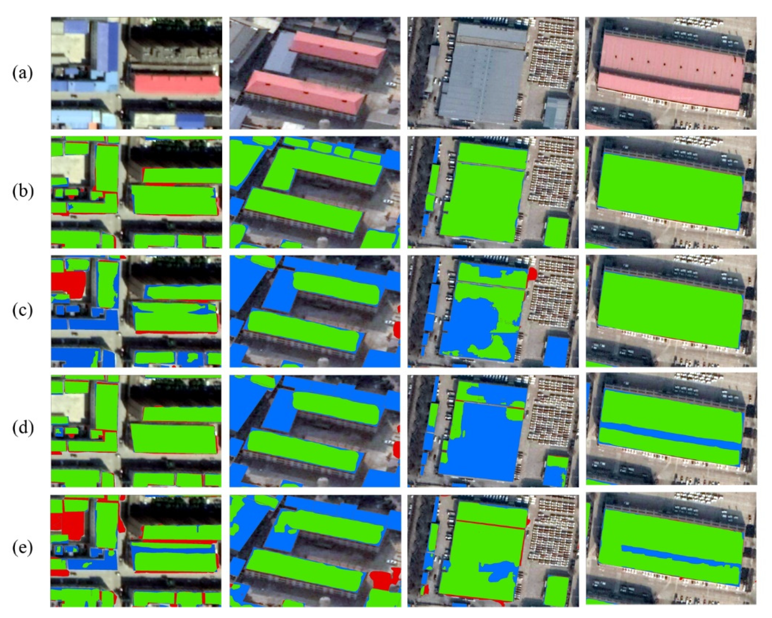
Table 4 shows that the extraction accuracy and recall rate of SENet for buildings of different colors are higher than those of the three individual models. We also found that the precision and recall rate for white and gray buildings are not very different from the average values, indicating that buildings of these two colors have little influence on the extraction accuracy of the four models. The precision and recall rate of the four models in extracting red buildings are 0.016, 0.071, 0.032, and 0.029 and 0.075, 0.083, 0.09, and 0.082 higher than the averages, respectively, indicating that the accuracies of the four models in extracting red buildings are higher than those in extracting buildings of other colors. The precision and recall rate when extracting blue buildings are lower than the average by 0.02, 0.061, 0.032, and 0.03 and 0.087, 0.087, 0.1, and 0.09, indicating that these four models have lower accuracies when extracting blue buildings. To show the difference more intuitively in the extraction accuracies of red and blue buildings, four samples of red and blue building data are selected from the test dataset. Figure 6 shows the extraction results of the four models on these four building samples.

Figure 6.
Segmentation results of the different methods for buildings of different colors. (a) Original input image. (b) The output of SENet. (c) The output of U-Net. (d) The output of SegNet. (e) The output of FCN-8s. The green, red, and blue pixels of the maps represent true positive, false positive and false negative predictions, respectively.
Figure 6 shows that all models have high accuracy when extracting red buildings. Only SegNet (Figure 6d) and FCN-8s (Figure 6e) exhibit false negatives (blue) in the middle shadow part of the red buildings in the fourth column. In Figure 6c,d, U-Net and SegNet have a large number of missed extractions when extracting blue buildings. The reason for this result is that the color difference between the blue buildings and the image background, which contains roads and ground, is small, which leads to the model easily misclassifying blue buildings as non-buildings. The color difference between the red buildings and the image background is large, so the extraction accuracy is high. After using CRFs to optimize the prediction results of the basic model, SENet showed good extraction performance for buildings of different colors.
3.3.3. Building Sizes
We calculate the accuracy of the extraction results for buildings of different sizes with different models. Precision and recall are still selected as evaluation indexes. Table 5 shows the accuracy evaluation indexes extracted by the four models for buildings of different sizes. SENet achieved the highest precision and recall values when extracting buildings of all different sizes compared with the other three individual models. For small buildings, the precision and recall values of the extraction results of the four models are greater than the average values. When extracting medium-sized buildings, the precision values of U-Net and FCN-8s are lower than the average value, which indicates that the two models produce more false-positive (red) pixels in the extraction of medium-sized buildings. When extracting large buildings, the recall value of FCN-8s is higher than the average value and is 10.6% and 8.8% higher than the U-Net and SegNet values, respectively, and the highest recall value of SENet is 0.897.
Table 5.
Quantitative results of different models for buildings of different sizes.
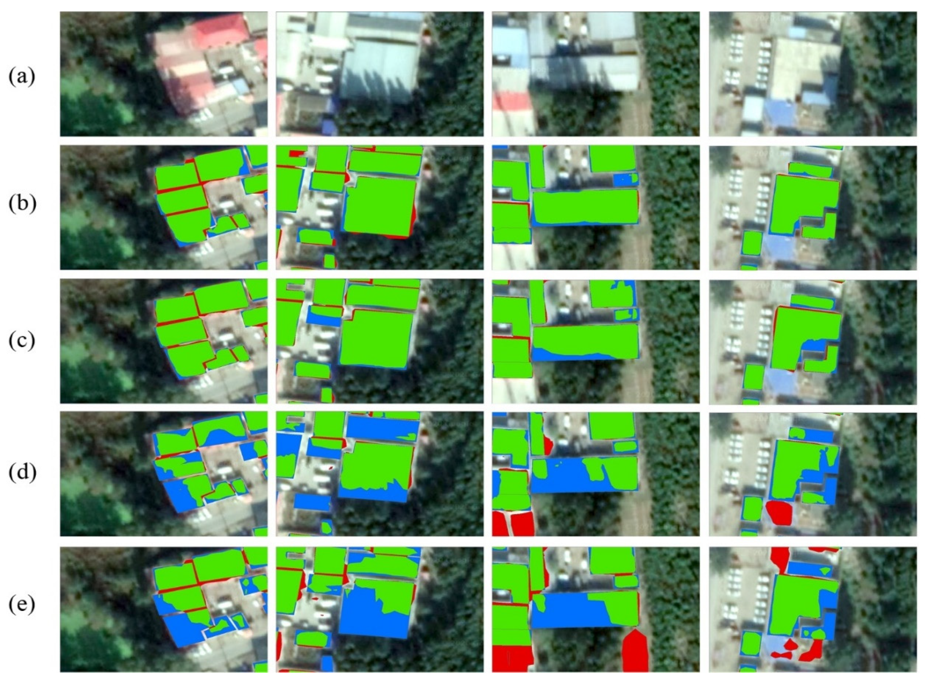
We select representative buildings from each category in the building dataset and classify them by size to visualize the extraction results. The results are shown in Figure 7. Among them, the area with small buildings is 160 m2, the area with medium buildings is 2323 m2, and the area with large buildings is 15,973 m2. To ensure that the contrast experiment is not affected by the color of the building roofs, we selected three buildings with similar colors.
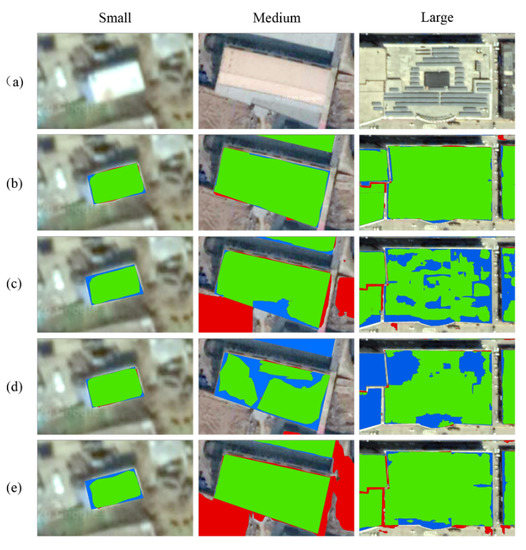
Figure 7.
Segmentation results of the different methods for buildings of different sizes. (a) Original input image. (b) The output of SENet. (c) The output of U-Net. (d) The output of SegNet. (e) The output of FCN-8s. The green, red, and blue pixels of the maps represent true positive, false positive and false negative predictions, respectively.
Figure 7 shows that for small buildings in the first column, the four models have achieved high extraction accuracies, especially the SENet and SegNet models, which produce very few false negatives (blue) and false positives (red). For medium-sized buildings, U-Net and SegNet produce a large number of false negatives (blue), and their extraction accuracies are reduced. SENet and FCN-8s produce fewer false negatives (blue), but FCN-8s produces a large area of false positives (red). For large buildings, U-Net and SegNet generate many missed detection holes, while FCN-8s produces fewer missed detections. SENet inherits the excellent features of FCN-8S when extracting large-scale buildings.
3.3.4. Building Shapes
For the feature attribute labels of the buildings, we use the structure and edge contours to describe the shape of a building. We selected buildings of different shapes from the prediction results of the test dataset for analysis, as shown in Figure 8. The first two columns of buildings in the picture are simple in structure, while the last two columns contain buildings that are complex. Among the four building samples, only the third column of buildings has blurry edge contours, while the remaining three buildings have obvious edge contours. The figure shows that SegNet has poor performance for building extraction, and there are a large number of false negatives (blue) on the four building samples. For the other two individual models, U-Net and FCN-8s have good extraction performance for simple buildings, such as those in the first and second columns. However, for the third column containing buildings with complex structures and blurry edge contours, all models failed to identify the boundaries of the buildings well, and many missing pixels appeared on the edges of the buildings. Although the building in the fourth column has a complex structure, its edges are obvious and significantly different from the surrounding roads. SENet and U-Net have high extraction precision outcomes on such buildings. For buildings of different shapes, the extraction results of SENet are better than those of the other three individual models.
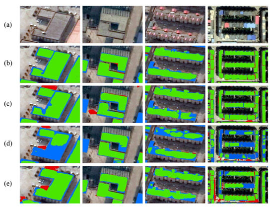
Figure 8.
Segmentation results of the different methods for buildings of different shapes. (a) Original input image. (b) The output of SENet. (c) The output of U-Net. (d) The output of SegNet. (e) The output of FCN-8s. The green, red, and blue pixels of the maps represent true positive, false positive and false negative predictions, respectively.
3.3.5. Building Shadows
According to the shadow attributes in the building-feature attribute tags, we found a total of 126 buildings covered by shadows from four test images and analyzed the extraction performance of the four models on these buildings. Building pixels covered by shadows are often misclassified as non-buildings. These misclassified results are considered false negatives (blue), so we use recall to evaluate the extraction performance. We define a single building with a recall value greater than or equal to 0.8 as a complete extraction and with a recall value less than 0.8 as an incomplete extraction. Among the 126 buildings covered by shadows, the SENet model completely extracted 121 buildings with the highest accuracy rate of 96.0%. The U-Net model completely extracted 107 buildings with an accuracy rate of 84.9%. SegNet completely extracted 13 buildings with an accuracy rate of 10.3%. FCN-8s only extracted four buildings
Completely with an accuracy rate of 3.2%. Figure 9 shows four of the 126 buildings covered by tree shadows and the extraction results of the different models. As shown in Figure 9d,e, SegNet and FCN-8s did not effectively extract the buildings covered by shadows, which are considered missed detections. U-Net extracted most of the area covered by shadows, and only a small number of missing pixels appeared. SENet effectively inherits the advantages of U-Net in extracting shadowed buildings and has the highest extraction accuracy.

Figure 9.
Segmentation results of the different methods for buildings covered by shadows. (a) Original input image. (b) The output of SENet. (c) The output of U-Net. (d) The output of SegNet. (e) The output of FCN-8s. The green, red, and blue pixels of the maps represent true positive, false positive and false negative predictions, respectively.
4. Discussion
In this section, the proposed model is discussed in five aspects. First, the established building dataset is compared with the other available public building datasets. In order to explore the applicability of the proposed SENet, we select another dataset to test the effectiveness of SENet. In addition, the processing time of different models is compared. An ablation study is also conducted to discuss the contributions of different models. Finally, the influence of the number of inference function calculations in the CRFS model on the optimization results is discussed in detail.
4.1. Dataset Evaluation
Currently, there are four open-source datasets commonly used for building extraction, namely the WHU dataset [53], ISPRS dataset, Massachusetts dataset [17], and Inria dataset [54]. Table 6 compares the dataset created in this paper with these datasets in terms of the coverage area, ground resolution, data source, image block size and number, and label format. The WHU dataset provides samples that contain both raster and vector data types from aerial and satellite sources. The ISPRS Vaihingen dataset and Potsdam dataset provide labels for semantic segmentation and consist of high-resolution orthophotographs and the corresponding digital surface models. However, the Vaihingen and Potsdam datasets cover only a very small ground range. The Massachusetts dataset covers 340 km2 but has a relatively low resolution. The ground resolution of the INRIA dataset is similar to the ground resolution of the dataset created in this article, but the coverage area is smaller than that of our dataset. Although our dataset is inferior to the WHU and ISPRS datasets in terms of ground resolution, our dataset has a larger coverage area and richer building sample types. In addition, our dataset is the only dataset among all the publicly available datasets that has attribute tags describing the features of each building.
Table 6.
Comparison of our dataset and the other open-source datasets.
4.2. Applicability Analysis of SENet
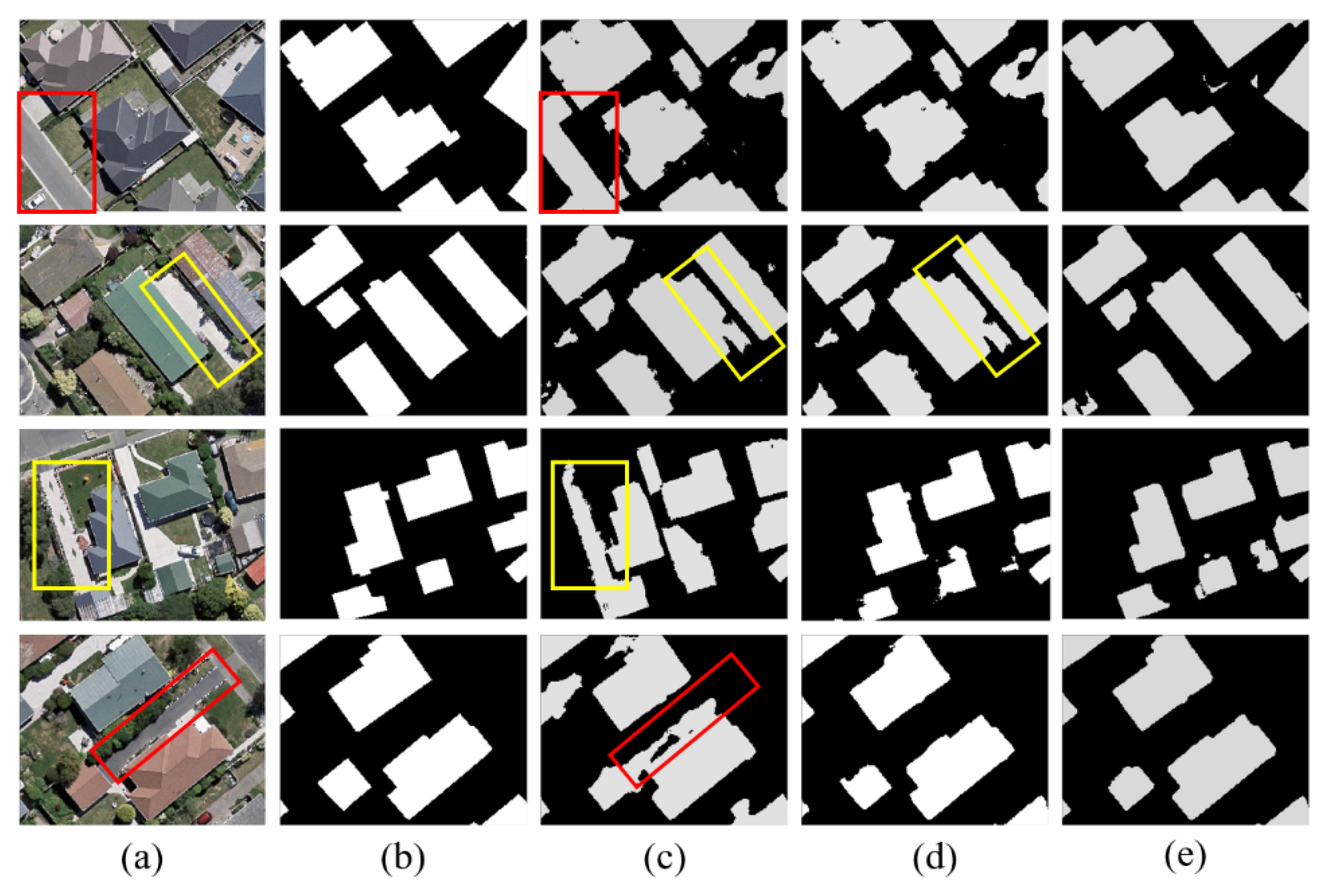
To further explore the applicability of SENet, the urban area of Waimakariri, New Zealand was used to test the effectiveness of SENet. The aerial images of Waimakariri were taken during 2015 and 2016, with a spatial resolution of 0.075 m. The corresponding building outlines were also provided by the website (https://data.linz.govt.nz, accessed on 29 August 2021). The results of the Waimakariri area are presented in Figure 10. The U-Net model misclassifies parts of roads as buildings (Figure 10c red rectangle). Both U-Net and SegNet misclassify hardened ground as buildings (Figure 10c,d yellow rectangle). It is obvious that SENet outperformed the other approaches. Quantitative results are provided in Table 7. The overall performance of SENet in this study was the best among deep models, followed by SegNet and U-Net. The performance of these deep models was basically consistent with the testing results of the dataset created in this article, indicating that SENet has high applicability and can be applied to other cities and rural areas.

Figure 10.
Segmentation results of the different methods for an urban area of Waimakariri, New Zealand. (a) Original input image. (b) Ground truth. (c) The output of U-Net. (d) The output of SegNet. (e) The output of SENet.
Table 7.
Quantitative comparison of four metrics (for an urban area of Waimakariri, New Zealand) obtained from the segmentation results by SegNet, U-Net and the proposed SENet.
4.3. Complexity Comparison of Deelp Learning Models
Computational cost is also a significant efficiency indicator in deep learning. It represents the complexity of the deep learning model where the costs for training and testing quantify the differences in complexity between CNN models. To evaluate the complexity of SENet, the training time and testing time were compared with five existing deep learning approaches (i.e., SegNet, FCN-8s, U-Net, DeconvNet, and DeepUNet). It is worthwhile mentioning that the running time of deep models including training and testing time can be affected by many factors, such as the structure and the model parameters. Here, we simply compared the complexity of deep models. As shown in Table 8, DeconvNet has the longest training time and testing time among all models. DeepUNet has the shortest training and testing time, because DeepUNet adopted a very small convolution channel (each convolutional layer with 32 channels). However, SENet requires a longer training time than SegNet, FCN-8s, and U-Net. The main reason for this is that the optimization and combination of the basic model requires a portion of the processing time. Compared with FCN-8s and SegNet, they require less training time than SENet, but the testing time of SENet is shorter than that of FCN-8s, close to that of SegNet. From the viewpoint of accuracy improvement and reducing computing resources, such a minor time increase should be acceptable. Overall, SENet achieves a relative trade-off between the model performance and complexity.
Table 8.
Complexity comparison of SegNet, FCN-8s, U-Net, DeconvNet, DeepUNet and the proposed SENet.
4.4. Ablation Study
As mentioned in Section 2, SENet is integrated by three basic models, including SegNet, FCN-8s and U-Net. To study their contributions to the building extraction task, we design five networks to complete the building extraction respectively. They are as follows:
- Net 1: SegNet
- Net 2: SegNet + FCN-8s
- Net 3: SegNet + U-Net
- Net 4: FCN-8s + U-Net
- Net 5: SegNet + FCN-8s + U-Net
Note that the experimental settings of the networks in this section are the same as those mentioned in Section 3.2. The results of these networks counted on the dataset are shown in Figure 11. From the observation of Figure 10, we can find that the performance of different networks is proportional to the number of basic models. In detail, the behavior of Net 1 is the weakest among all compared networks since it only consists of a basic model SegNet. After integrating two basic models, the performances of Net 2, Net 3, and Net 4 are stronger than that of Net 1. Integrating all three basic models, Net 5 achieves the best performance. Furthermore, the performance gap between Net 5 and other networks is distinct. The results discussed above demonstrate that each basic models can make a positive contribution to our SENet model, and integrating three basic model achieves an incremental improvement over two.
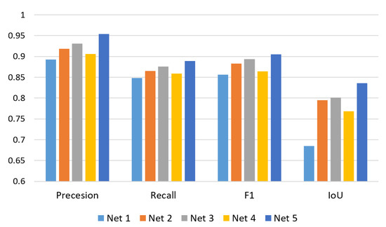
Figure 11.
Ablation Study for the proposed SENet.
4.5. Analysis of the Number of CRF Optimization Calculations
The most important step in the CRF model is to use the inference function to perform inference operations to obtain the value of the energy function. Each additional operation will reduce the energy so that the segmentation results are closer to the color information of the real objects. Although the color information of buildings can be used to improve the edge segmentation effect of buildings, overinference is also likely to increase segmentation result errors due to the interference of color information, resulting in overclassification. To explore the number of inference function estimation calculations required to obtain the optimal segmentation result, experiments with 0–7 calculations were carried out. Taking the segmentation optimization of residential buildings as an example, the effect is shown in Figure 12.
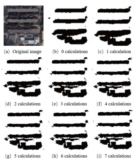
Figure 12.
Optimization effect under different calculation numbers.
Figure 10 shows that a better optimization effect can be reached after four calculations. In addition to the complex color information of buildings on the south side, which leads to a poor segmentation effect, the boundary segmentation result has been optimized according to a certain amount of color information, and the postsegmentation operation has been completed well. In the fifth inference, the image is influenced by more color information, resulting in oversegmentation. Therefore, in this study, the four-calculation inference CRF model is used to optimize the base model to achieve the best optimization effect.
5. Conclusions
To integrate the feature advantages of different deep learning models and improve the robustness and stability of the model, a deep learning feature integration method based on a stacking ensemble technique was proposed for extracting buildings from remote sensing images. The proposed SENet model was compared with three individual CNN models (U-NET, SegNet and FCN-8s) on the dataset created in this paper. By adding feature attribute tags to the buildings in the test set, it is verified that the proposed model can effectively integrate the feature advantages of different models. To ensure the fairness and reliability of the experiment, the same training data and training parameters were used. Four widely used statistical metrics were selected for evaluating the extraction performance of the model. The experimental results show that the accuracy, recall, F1 score, and IoU of the proposed SENet on the test dataset reached 0.954, 0.889, 0.905, and 0.75, respectively, which are all superior to those of the three individual CNN models (U-net, SegNet and FCN-8s). The proposed SENet can effectively integrate the feature advantages of different models and obtain excellent prediction results when extracting buildings of different colors, sizes, and shapes and buildings with shadows. The prediction results will form an important information source for environmental observations.
Although the proposed model can achieve satisfactory extraction results, limitations still exist. First, the proposed model requires more computation time, memory, and resources than the individual models in the construction and combination stages of the basic predictors. Therefore, more effective strategies for the construction and combination of basic models must be explored to further enhance the computational efficiency and scalability of the model. Second, the proposed model also needs to be tested on other public building datasets to verify its generalization ability on different datasets.
Author Contributions
Conceptualization, D.C. and H.X.(Hanfa Xing); methodology, software, and validation, D.C., H.X. (Hanfa Xing) and Y.M.; formal analysis, D.C.; writing—original draft preparation, D.C.; writing—review and editing, H.X. (Hanfa Xing), M.S.W., M.-P.K., H.X. (Huaqiao Xing) and Y.M.; project administration, H.X. (Hanfa Xing); funding acquisition, H.X. (Hanfa Xing) All authors have read and agreed to the published version of the manuscript.
Funding
Hanfa Xing thanks the funding support from a grant by the National Natural Science Foundation of China (Grant no. 41971406). Man Sing Wong thanks the funding support from a grant by the General Research Fund (Grant no. 15602619), the Collaborative Research Fund (Grant no. C7064-18GF), and the Research Institute for Sustainable Urban Development (Grant no. 1-BBWD), the Hong Kong Polytechnic University. Mei-Po Kwan was supported by grants from the Hong Kong Research Grants Council (General Research Fund Grant no. 14605920; Collaborative Research Fund Grant no. C4023-20GF) and a grant from the Research Committee on Research Sustainability of Major Research Grants Council Funding Schemes of the Chinese University of Hong Kong.
Data Availability Statement
Not applicable.
Acknowledgments
The authors are grateful to the Editor and reviewers for their constructive comments, which significantly improved this work.
Conflicts of Interest
The authors declare no conflict of interest.
References
- Ghanea, M.; Moallem, P.; Momeni, M. Building extraction from high-resolution satellite images in urban areas: Recent methods and strategies against significant challenges. Int. J. Remote Sens. 2016, 37, 5234–5248. [Google Scholar] [CrossRef]
- Grinias, I.; Panagiotakis, C.; Tziritas, G. MRF-based segmentation and unsupervised classification for building and road detection in peri-urban areas of high-resolution satellite images. ISPRS J. Photogramm. Remote Sens. 2016, 122, 145–166. [Google Scholar] [CrossRef]
- Chen, R.; Li, X.; Li, J. Object-Based Features for House Detection from RGB High-Resolution Images. Remote Sens. 2018, 10, 451. [Google Scholar] [CrossRef] [Green Version]
- Hui, J.; Du, M.; Ye, X.; Qin, Q.; Sui, J. Effective Building Extraction From High-Resolution Remote Sensing Images With Multitask Driven Deep Neural Network. IEEE Geosci. Remote Sens. Lett. 2018, 16, 786–790. [Google Scholar] [CrossRef]
- Jing, W.; Xu, Z.; Ying, L. Texture-based segmentation for extracting image shape features. In Proceedings of the 2013 19th International Conference on Automation and Computing (ICAC), London, UK, 13–14 September 2013. [Google Scholar]
- Lowe, D.G. Distinctive Image Features from Scale-Invariant Keypoints. Int. J. Comput. Vis. 2004, 60, 91–110. [Google Scholar] [CrossRef]
- Ojala, T.; Pietikainen, M.; Maenpaa, T. Multiresolution gray-scale and rotation invariant texture classification with local binary patterns. IEEE Trans. Pattern Anal. Mach. Intell. 2002, 24, 971–987. [Google Scholar] [CrossRef]
- Dalal, N.; Triggs, B. Histograms of Oriented Gradients for Human Detection. In Proceedings of the IEEE Computer Society Conference on Computer Vision and Pattern Recognition, San Diego, CA, USA, 20–25 June 2005; Volume 1, pp. 886–893. [Google Scholar] [CrossRef] [Green Version]
- Inglada, J. Automatic recognition of man-made objects in high resolution optical remote sensing images by SVM classification of geometric image features. ISPRS J. Photogramm. Remote Sens. 2007, 62, 236–248. [Google Scholar] [CrossRef]
- Aytekin, Ö.; Zongur, U.; Halici, U. Texture-Based Airport Runway Detection. IEEE Geosci. Remote Sens. Lett. 2012, 10, 471–475. [Google Scholar] [CrossRef]
- Dong, Y.; Du, B.; Zhang, L. Target Detection Based on Random Forest Metric Learning. IEEE J. Sel. Top. Appl. Earth Obs. Remote Sens. 2015, 8, 1830–1838. [Google Scholar] [CrossRef]
- Li, E.; Femiani, J.; Xu, S.; Zhang, X.; Wonka, P. Robust Rooftop Extraction From Visible Band Images Using Higher Order CRF. IEEE Trans. Geosci. Remote Sens. 2015, 53, 4483–4495. [Google Scholar] [CrossRef]
- Long, J.; Shelhamer, E.; Darrell, T. Fully convolutional networks for semantic segmentation. arXiv 2014, arXiv:1411.4038. [Google Scholar]
- Badrinarayanan, V.; Kendall, A.; Cipolla, R. SegNet: A Deep Convolutional Encoder-Decoder Architecture for Image Segmentation. IEEE Trans. Pattern Anal. Mach. Intell. 2017, 39, 2481–2495. [Google Scholar] [CrossRef] [PubMed]
- Ronneberger, O.; Fischer, P.; Brox, T. U-Net: Convolutional Networks for Biomedical Image Segmentation. arXiv 2015, arXiv:1505.04597. [Google Scholar]
- Chaurasia, A.; Culurciello, E. LinkNet: Exploiting encoder representations for efficient semantic segmentation. In Proceedings of the 2017 IEEE Visual Communications and Image Processing (VCIP), Saint Petersburg, FL, USA, 10–13 December 2017; pp. 1–4. [Google Scholar]
- Mnih, V. Machine Learning for Aerial Image Labeling; University of Toronto: Toronto, ON, Canada, 2013. [Google Scholar]
- Saito, S.; Yamashita, T.; Aoki, Y. Multiple Object Extraction from Aerial Imagery with Convolutional Neural Networks. J. Imaging Sci. Technol. 2016, 60, 104021–104029. [Google Scholar] [CrossRef]
- Bittner, K.; Adam, F.; Cui, S.; Korner, M.; Reinartz, P. Building Footprint Extraction From VHR Remote Sensing Images Combined With Normalized DSMs Using Fused Fully Convolutional Networks. IEEE J. Sel. Top. Appl. Earth Obs. Remote Sens. 2018, 11, 2615–2629. [Google Scholar] [CrossRef] [Green Version]
- Yi, Y.; Zhang, Z.; Zhang, W.; Zhang, C.; Li, W.; Zhao, T. Semantic Segmentation of Urban Buildings from VHR Remote Sensing Imagery Using a Deep Convolutional Neural Network. Remote Sens. 2019, 11, 1774. [Google Scholar] [CrossRef] [Green Version]
- Noh, H.; Hong, S.; Han, B. Learning deconvolution network for semantic segmentation. In Proceedings of the IEEE International Conference on Computer Vision, Santiago, Chile, 7–13 December 2015; pp. 1520–1528. [Google Scholar]
- Zhang, Z.; Liu, Q.; Wang, Y. Road Extraction by Deep Residual U-Net. IEEE Geosci. Remote Sens. Lett. 2018, 15, 749–753. [Google Scholar] [CrossRef] [Green Version]
- Li, R.; Liu, W.; Yang, L.; Sun, S.; Hu, W.; Zhang, F.; Li, W. DeepUNet: A Deep Fully Convolutional Network for Pixel-Level Sea-Land Segmentation. IEEE J. Sel. Top. Appl. Earth Obs. Remote Sens. 2018, 11, 3954–3962. [Google Scholar] [CrossRef] [Green Version]
- Pan, X.; Yang, F.; Gao, L.; Chen, Z.; Zhang, B.; Fan, H.; Ren, J. Building Extraction from High-Resolution Aerial Imagery Using a Generative Adversarial Network with Spatial and Channel Attention Mechanisms. Remote Sens. 2019, 11, 917. [Google Scholar] [CrossRef] [Green Version]
- Ye, Z.; Fu, Y.; Gan, M.; Deng, J.; Comber, A.; Wang, K. Building Extraction from Very High Resolution Aerial Imagery Using Joint Attention Deep Neural Network. Remote Sens. 2019, 11, 2970. [Google Scholar] [CrossRef] [Green Version]
- Lin, G.; Milan, A.; Shen, C.; Reid, I. RefineNet: Multi-path Refinement Networks for High-Resolution Semantic Segmentation. In Proceedings of the IEEE Conference on Computer Vision and Pattern Recognition, Honolulu, HI, USA, 21–26 July 2017; pp. 5168–5177. [Google Scholar] [CrossRef] [Green Version]
- Jegou, S.; Drozdzal, M.; Vazquez, D.; Romero, A.; Bengio, Y. The one hundred layers tiramisu: Fully convolutional DenseNets for semantic segmentation. In Proceedings of the IEEE Computer Society Conference on Computer Vision and Pattern Recognition Workshops, Honolulu, HI, USA, 21–26 July 2017; pp. 1175–1183. [Google Scholar]
- Liu, P.; Liu, X.; Liu, M.; Shi, Q.; Yang, J.; Xu, X.; Zhang, Y. Building Footprint Extraction from High-Resolution Images via Spatial Residual Inception Convolutional Neural Network. Remote Sens. 2019, 11, 830. [Google Scholar] [CrossRef] [Green Version]
- Lin, L.; Jian, L.; Min, W.; Zhu, H. A Multiple-Feature Reuse Network to Extract Buildings from Remote Sensing Imagery. Remote Sens. 2018, 10, 1350. [Google Scholar]
- Liu, W.; Yang, M.; Xie, M.; Guo, Z.; Li, E.; Zhang, L.; Pei, T.; Wang, D. Accurate Building Extraction from Fused DSM and UAV Images Using a Chain Fully Convolutional Neural Network. Remote Sens. 2019, 11, 2912. [Google Scholar] [CrossRef] [Green Version]
- Zhang, S.; Chen, Y.; Zhang, W.; Feng, R. A novel ensemble deep learning model with dynamic error correction and multi-objective ensemble pruning for time series forecasting—ScienceDirect. Inf. Sci. 2021, 544, 427–445. [Google Scholar] [CrossRef]
- Ma, J.; Wu, L.; Tang, X.; Liu, F.; Zhang, X.; Jiao, L. Building Extraction of Aerial Images by a Global and Multi-Scale Encoder-Decoder Network. Remote Sens. 2020, 12, 2350. [Google Scholar] [CrossRef]
- Ju, M.; Ding, C.; Ren, W.; Yang, Y.; Zhang, D.; Guo, Y.J. IDE: Image Dehazing and Exposure Using an Enhanced Atmospheric Scattering Model. IEEE Trans. Image Process. 2021, 30, 2180–2192. [Google Scholar] [CrossRef] [PubMed]
- Ju, M.; Ding, C.; Guo, Y.J.; Zhang, D. IDGCP: Image Dehazing Based on Gamma Correction Prior. IEEE Trans. Image Process. 2020, 29, 3104–3118. [Google Scholar] [CrossRef] [PubMed]
- Shao, H.; Jiang, H.; Lin, Y.; Li, X. A novel method for intelligent fault diagnosis of rolling bearings using ensemble deep auto-encoders. Mech. Syst. Signal Process. 2018, 102, 278–297. [Google Scholar] [CrossRef]
- Zhou, J.; Peng, T.; Zhang, C.; Sun, N. Data Pre-Analysis and Ensemble of Various Artificial Neural Networks for Monthly Streamflow Forecasting. Water 2018, 10, 628. [Google Scholar] [CrossRef] [Green Version]
- David, B. Online cross-validation-based ensemble learning. Stat. Med. 2018, 2, 37. [Google Scholar]
- Sun, G.; Huang, H.; Zhang, A.; Li, F.; Zhao, H.; Fu, H. Fusion of Multiscale Convolutional Neural Networks for Building Extraction in Very High-Resolution Images. Remote Sens. 2019, 11, 227. [Google Scholar] [CrossRef] [Green Version]
- Saqlain, M.; Jargalsaikhan, B.; Lee, J.Y. A Voting Ensemble Classifier for Wafer Map Defect Patterns Identification in Semiconductor Manufacturing. IEEE Trans. Semicond. Manuf. 2019, 32, 171–182. [Google Scholar] [CrossRef]
- Cheng, J.; Aurélien, B.; van der, L.M. The relative performance of ensemble methods with deep convolutional neural networks for image classification. J. Appl. Stat. 2018, 45, 2800–2818. [Google Scholar]
- Gong, M.; Liu, J.; Li, H.; Cai, Q.; Su, L. A Multiobjective Sparse Feature Learning Model for Deep Neural Networks. IEEE Trans. Neural Networks Learn. Syst. 2015, 26, 3263–3277. [Google Scholar] [CrossRef]
- Huang, B.; Lu, K.; Audeberr, N.; Khalel, A.; Tarabalka, Y.; Malof, J.; Boulch, A.; Le Saux, B.; Collins, L.; Bradbury, K.; et al. Large-Scale Semantic Classification: Outcome of the First Year of Inria Aerial Image Labeling Benchmark. In Proceedings of the IGARSS 2018—2018 IEEE International Geoscience and Remote Sensing Symposium, Valencia, Spain, 22–27 July 2018; pp. 6947–6950. [Google Scholar]
- Simonyan, K.; Zisserman, A. Very deep convolutional networks for large-scale image recognition. arXiv 2014, arXiv:1409.1556. [Google Scholar]
- Bischke, B.; Helber, P.; Folz, J.; Borth, D.; Dengel, A. Multi-Task Learning for Segmentation of Building Footprints with Deep Neural Networks. In Proceedings of the 2019 IEEE International Conference on Image Processing (ICIP), Taipei, Taiwan, 22–25 September 2019; pp. 1480–1484. [Google Scholar] [CrossRef] [Green Version]
- Krähenbühl, P.; Koltun, V. Efficient Inference in Fully Connected CRFs with Gaussian Edge Potentials. Adv. Neural Inf. Process. Syst. 2012, 24, 10–20. [Google Scholar]
- Zhang, B.; Wang, C.; Shen, Y.; Liu, Y. Fully Connected Conditional Random Fields for High-Resolution Remote Sensing Land Use/Land Cover Classification with Convolutional Neural Networks. Remote Sens. 2018, 10, 1889. [Google Scholar] [CrossRef] [Green Version]
- Orlando, J.I.; Prokofyeva, E.; Blaschko, M. A Discriminatively Trained Fully Connected Conditional Random Field Model for Blood Vessel Segmentation in Fundus Images. IEEE Trans. Biomed. Eng. 2016, 64, 16–27. [Google Scholar] [CrossRef] [PubMed] [Green Version]
- Wagner, S.A. SAR ATR by a combination of convolutional neural network and support vector machines. IEEE Trans. Aerosp. Electron. Syst. 2016, 52, 2861–2872. [Google Scholar] [CrossRef]
- Szegedy, C.; Liu, W.; Jia, Y.; Sermanet, P.; Reed, S.; Anguelov, D.; Erhan, D.; Vanhoucke, V.; Rabinovich, A. Going deeper with convolutions. In Proceedings of the 2015 IEEE Conference on Computer Vision and Pattern Recognition (CVPR), Boston, MA, USA, 7–12 June 2015; pp. 1–9. [Google Scholar]
- Zhang, Y.; Gong, W.; Sun, J.; Li, W. Web-Net: A Novel Nest Networks with Ultra-Hierarchical Sampling for Building Extraction from Aerial Imageries. Remote Sens. 2019, 11, 1897. [Google Scholar] [CrossRef] [Green Version]
- Castagno, J.; Atkins, E. Roof Shape Classification from LiDAR and Satellite Image Data Fusion Using Supervised Learning. Sensors 2018, 18, 3960. [Google Scholar] [CrossRef] [PubMed] [Green Version]
- Gabay, H.; Meir, I.A.; Schwartz, M.; Werzberger, E. Cost-benefit analysis of green buildings: An Israeli office buildings case study. Energy Build. 2014, 76, 558–564. [Google Scholar] [CrossRef]
- Ji, S.; Wei, S.; Lu, M. Fully Convolutional Networks for Multisource Building Extraction From an Open Aerial and Satellite Imagery Data Set. IEEE Trans. Geosci. Remote Sens. 2019, 57, 574–586. [Google Scholar] [CrossRef]
- Maggiori, E.; Tarabalka, Y.; Charpiat, G.; Alliez, P. Can semantic labeling methods generalize to any city? The inria aerial image labeling benchmark. In Proceedings of the 2017 IEEE International Geoscience and Remote Sensing Symposium (IGARSS), Fort Worth, TX, USA, 23–28 July 2017; pp. 3226–3229. [Google Scholar]


Publisher’s Note: MDPI stays neutral with regard to jurisdictional claims in published maps and institutional affiliations. |
© 2021 by the authors. Licensee MDPI, Basel, Switzerland. This article is an open access article distributed under the terms and conditions of the Creative Commons Attribution (CC BY) license (https://creativecommons.org/licenses/by/4.0/).