Article

Camouflaged Target Detection Based on Snapshot Multispectral Imaging

School of Mechanical Engineering and Automation, Fuzhou University, Fuzhou 350108, China
*
Author to whom correspondence should be addressed.
Remote Sens. 2021, 13(19), 3949; https://doi.org/10.3390/rs13193949
Submission received: 22 July 2021 / Revised: 21 September 2021 / Accepted: 29 September 2021 / Published: 2 October 2021
(This article belongs to the Special Issue Applications of Remote Sensing Imagery for Urban Areas)

Abstract

:
The spectral information contained in the hyperspectral images (HSI) distinguishes the intrinsic properties of a target from the background, which is widely used in remote sensing. However, the low imaging speed and high data redundancy caused by the high spectral resolution of imaging spectrometers limit their application in scenarios with the real-time requirement. In this work, we achieve the precise detection of camouflaged targets based on snapshot multispectral imaging technology and band selection methods in urban-related scenes. Specifically, the camouflaged target detection algorithm combines the constrained energy minimization (CEM) algorithm and the improved maximum between-class variance (OTSU) algorithm (t-OTSU), which is proposed to obtain the initial target detection results and adaptively segment the target region. Moreover, an object region extraction (ORE) algorithm is proposed to obtain a complete target contour that improves the target detection capability of multispectral images (MSI). The experimental results show that the proposed algorithm has the ability to detect different camouflaged targets by using only four bands. The detection accuracy is above 99%, and the false alarm rate is below 0.2%. The research achieves the effective detection of camouflaged targets and has the potential to provide a new means for real-time multispectral sensing in complex scenes.

1. Introduction

Hyperspectral target detection is widely used in industry, agriculture, and urban remote sensing [1]. Hyperspectral images (HSI) are often presented as spectral data cubes measured for each pixel as a spectral vector. The elements in the spectral vector correspond to the reflectance or radiation value in different spectral bands [2]. Therefore, it is possible to detect the camouflaged targets based on the spectral characteristic of the target materials [3]. Manolakis, Shaw, and other researchers [4,5,6,7] in MIT’s Lincoln laboratory summarized the detection algorithms that exploit spectral information and argued that the “apparent” superiority of sophisticated algorithms with simulated data or in laboratory conditions did not necessarily translate to superiority in real-world applications. From the perspective of military defense and reconnaissance applications, they proposed to improve the performance of detection algorithms by solving the problem of the inherent variability target and background spectra (i.e., the mismatch between the spectral library and in-scene signatures) [5,7]. In addition, many other scholars made relevant contributions. Yan [8] and Hua [9] et al. successfully used the constrained energy minimization (CEM) [10] algorithm and the adaptive coherence estimator (ACE) [6] algorithm to detect the camouflaged targets in real-world scenarios. Kumar et al. [11] used unsupervised target detection algorithms, including the K-means classification method, the Reed–Xiaoli (RX) algorithm, and the Iterative Self Organizing Data Analysis Technique Algorithm (ISODATA) to detect various camouflaged targets in mid-wave infrared HSIs.
However, the slow imaging speed of currently available spectral imagers and the “Hughes phenomenon”, which is induced due to the high dimensionality of data, limit the usage of HSI in applications with a high real-time requirement [12]. To address the problem of data redundancy in HSI, many researchers worked on dimensionality reduction (band selection) in HSI [13,14,15,16]. The main idea of band selection is to identify a representative set of bands among the spectral components with high correlation. The optimal clustering framework (OCF) [14], the multi-objective optimization band selection (MOBS) method [15], and the scalable one-pass self-representation learning (SOP-SRL) framework [16] are effective band selection methods.
Different from preserving the spectral features of substances through band selection, some researchers [17,18,19,20] focused on including the spatial features in the image analysis, which can be used for modeling the objects in the scene and increasing the discriminability between different thematic classes. Kwan and Ayhan et al. [21,22] demonstrated the effectiveness of Extended Multi-Attribute Profiles (EMAP) through extensive experiments. They also applied the Convolutional Neural Network (CNN)-based deep learning algorithms to spectral images enhanced with the EMAP, which achieve better land cover classification performance using only four bands as compared to that using all 144 hyperspectral bands [22]. However, this method generated additional augmented bands, consuming large amounts of computing resources and increasing the running time [21,22].
Additionally, the data redundancy problem also can be solved by determining several characteristic bands. Zhang [23], Liu [24], and Tian [25] et al. experimentally determined the characteristic bands of jungle camouflaged materials and white snow camouflaged materials as 680–720 nm and 330–380 nm, respectively. Afterward, the rapid identification of camouflaged targets was achieved with a common camera and the corresponding spectral filters. This method has high real-time performance and simple implementation. However, it requires more necessary prior knowledge to successfully detect specific targets and has narrow applications.
In order to achieve real-time spectral imaging, a filter array consisting of interferometric devices in multispectral imagers was designed to obtain spectral images containing corresponding bands [26,27]. A snapshot multispectral camera was manufactured by XIMEA, in conjunction with the Interuniversity Microelectronics Centre (IMEC) to quickly obtain multispectral images (MSIs). It integrates the pixel-level Fabry–Pérot filter mosaic array on the CMOS chip of an existing industrial camera, which improves the imaging speed. Contrary to the traditional multispectral imaging equipment, which obtains MSI at discrete time points, this snapshot multispectral camera extends spectral imaging to a broader field, such as dynamic video [28]. However, it is still a challenging problem to accurately detect the targets by limited multispectral bands.
Usually, a balance between the detection accuracy and the characteristic band numbers is of great significance in the application of targets detection in urban scenarios. In this work, based on the snapshot spectral imaging, we introduce the OCF algorithm to determine several general-purpose bands for the detection of camouflaged targets, so as to reduce the consumption of computing resources. We also propose a camouflaged target detection method based on CEM and an improved maximum between-class variance (OTSU) algorithm (t-OTSU). The CEM algorithm requires only prior spectral information to efficiently detect different camouflaged targets with low computational resource consumption, which applies well to our requirement. The proposed t-OTSU algorithm that overcomes the defect of the traditional OTSU algorithm is used to adaptively segment the target region from the output of the CEM detector in different scenarios. To eliminate the influence of misjudged regions contiguous to the target region, the object region extraction (ORE) algorithm is also proposed to obtain a complete contour of a camouflaged target.

2. Methodology

In this section, a detailed introduction of the proposed algorithm is presented. Figure 1 shows the flow chart of the proposed algorithm.

2.1. Calibration

The snapshot multispectral camera (MQ022HG-IM-SM5X5-NIR, XIMEA) with a spectral range of 670–975 nm is used to acquire the raw multispectral images ( I r a w ). Then, the raw images ( I r a w ) are corrected by using the white and dark references to reduce the spatial intensity variation of light and the dark current effect of the CMOS camera. The corrected multispectral image ( I M S I ) can be calculated as follows:
I M S I = I r a w I b l a c k _ r e f I w h i t e _ r e f I b l a c k _ r e f
where I b l a c k _ r e f and I w h i t e _ r e f represent a dark and a white reference, respectively.

2.2. CEM Detector

The CEM [10] detector is equivalent to an adaptive filter to pass the desired target with a specific gain, while the filter output resulting from unknown signal sources can be minimized, which can be used in camouflaged target reconnaissance. The MSI with N spectral vectors and D bands is expressed as a D × N matrix X = [ x 1 , x 2 , x 3 , , x N ] , and the spectrum of the target is represented as a D × 1 vector d . The main idea of the CEM algorithm, i.e., designing a finite impulse response (FIR) linear filter W = [ ω 1 , ω 2 , , ω N ] T , is implemented based on the MSI X and the prior known target spectrum vector d . Therefore, the output of CEM is described as the inner product of the spectral vector x and the FIR filter W as:
y = W T x .
The average energy output is expressed as:
1 N y 2 2 = 1 N W T x 2 2 = 1 N W T x x T W = W T R W
where R = ( 1 / N ) X X T denotes the correlation matrix of the MSI and y = [ y 1 , y 2 , , y N ] represents the output of the CEM detector.
By highlighting the target pixel while suppressing the “energy” of the background pixel, the CEM detector in the spectral space can separate the target from the background.
min W E { y 2 } = W T R W s . t .   W T d = 1
The filter is obtained as:
W C E M = R 1 d d T R 1 d .
The resultant target detection is expressed by the following mathematical expression.
y = ( W C E M ) T X = d T R 1 d R 1 d T X
After CEM treatment, the target is separated by using a threshold segmentation [8]. However, we observe that the results are significantly affected by the spectrum resolution. It is difficult to obtain a complete camouflaged target when the spectral bands are significantly reduced. To effectively address this problem, we propose an improved OTSU algorithm (t-OTSU).

2.3. Improved OTSU Algorithm (t-OTSU)

The traditional OTSU is an adaptive threshold segmentation algorithm, which is sensitive to the object size [29,30]. It is noteworthy that in the long-distance reconnaissance scenes, the proportion of the target pixels is much smaller than the background. Therefore, a large number of interferential areas are generated when OTSU is directly applied to the output of the CEM detector. The t-OTSU algorithm was proposed to eliminate the influence of object size. At the same time, by setting the value of the parameter t , we can avoid the phenomenon of false detection in the scene without camouflage target, to alert us to change the scene to search for targets.
Based on the traditional OTSU algorithm, we set the parameter t to determine the final adaptive threshold. We divide the pixels in the output of the CEM detector into two categories (i.e., C 0   and   C 1 ) based on a threshold T   ( 1 T M ) , where the output of the CEM detector ( I ) is represented in M gray levels. C 0 represents the set of background pixels, and C 1 represents the target. The probability of background and target pixels is p 1   and   p 2 , respectively. This is mathematically expressed by the following expression.
p 1 = i = 1 T p i p 2 = 1 p 1
where p i denotes the probability of the i th gray-level pixels, and
p i = n i N
where n i denotes the number of pixels at the i th gray level and N   ( N   =   n 1 + n 2 + + n M ) represents the total number of pixels.
Suppose m 1 and m 2 denote the mean values of the two categories, respectively; then, the overall mean m G of the image is expressed as:
m 1 = 1 / p 1 i = 1 T i p i m 2 = 1 / p 2 i = T + 1 M i p i m G = i = 1 M i p i
p 1 m 1 + p 2 m 2 = m G .
Similar to variance, the between-class variance is computed by the following relation.
σ 2 = p 1 ( m 1 m G ) 2 + p 2 ( m 2 m G ) 2
Based on Equations (7) and (8), the σ 2 is further expressed as:
σ 2 = p 1 p 2 ( m 1 m 2 ) 2 = ( m G p 1 i = 1 T i p i ) p 1 ( 1 p 1 ) .
The optimal threshold T * is defined as:
σ 2 ( T * ) = max { σ 2 } s . t .   1 T * M .
The parameter t is set to limit the value T to avoid the interference caused by the target size. The final result is expressed as follows:
T = { t 1 <   T * < t T * t <   T * < M .
The proposed t-OTSU algorithm is designed to segment the target region while minimizing the misclassified background pixels. However, there are still some misclassified regions around the target region. To solve this problem, we propose the following object region extraction (ORE) algorithm.

2.4. Object Region Extraction (ORE)

The opening operator can be used to separate the regular target region and the connected cluttered background areas, which does not affect the contour integrity of the target [31]. Thus, the ORE algorithm based on morphological operations [32] is proposed to eliminate the interferential regions. In our work, we use a disk structural element of radius 1 to separate the target region from the connected cluttered background area without affecting the contour integrity of the target.
The morphological “opening” is the combination of “erosion” and “dilation”, which is utilized to smooth the contours of large object regions while eliminating small free regions.
The erosion is similar to the convolution operation. We slide the structural element ( S E ) on the binary image I t O T S U , and the minimum value of the pixels in the overlapping area of the S E and I t O T S U is assigned to the corresponding anchor point position as the output value. This is expressed as follows:
I t O T S U S E = { x , y | ( S E ) x y I t O T S U }
where (x, y) denotes the corresponding position of anchor points, which is the center of S E .
Contrary, in dilation, the maximum value of pixels in overlapping areas is used as the output of the corresponding anchor point position as:
I t O T S U S E = { x , y | ( S E ) x y I t O T S U Ø } .
The morphological opening is the superposition of erosion and dilation and is expressed as follows:
I o = I t O T S U S E = ( I t O T S U S E ) S E .
The total number of independent regions in the binary image ( I o ), denoted as A , is determined based on the “n-Neighborhood” theory. Then, the regions are marked as R i ( i = 1 , 2 , 3 , , A ). Then, we record the number of the salient points within each area, and the area R J with the most pixels is selected. The salient points in the region R J are retained, whereas the rest of the areas are excluded to obtain a complete object region without interferential areas.

2.5. Evaluation Metrics

We use the false alarm ( F a ), accuracy ( A C ), and F1 measure ( F 1 ) as the evaluation metrics to quantitatively evaluate the performance of algorithms [33,34], which are expressed as follows:
F a = N F P N T P + N F P A C = N T P + N T N N
where N T N and N F P denote the number of background pixels that are correctly and incorrectly classified, respectively. N T P denotes the number of target pixels classified correctly, and N F N denotes the number of misclassified target pixels.
F 1 is mathematically expressed as:
F 1 = 2 P r e R e c P r e + R e c
where P r e and R c a l l represent the precision and recall, respectively. These quantities are mathematically expressed as:
P r e = N T P N T P + N F P R c a l l = N T P N T P + N F N .
Now, the F 1 is simplified as:
  F 1 = 2 N T P 2 N T P + N F P + N F N .
The ideal value of the index A C , which indicates that the proportion of correctly classified pixels is 1. Contrary, F a is a negative evaluation index, which is expected to approach 0 indefinitely. The F 1 is similar to A C ; however, it is considered more accurate.

3. Results

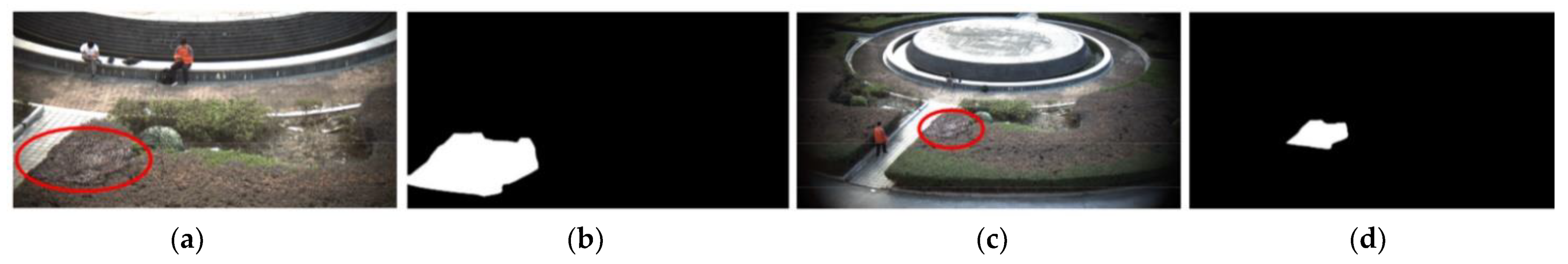
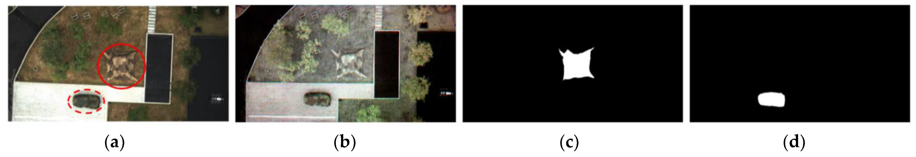
3.1. Experimental Scenarios

We obtain the original images by using a snapshot multispectral imager (MQ022HG-IM-SM5X5-NIR, XIMEA), as depicted in Figure 2a. This device contains 25 wavelength-specific Fabry–Pérot filters ranging from 660 to 975 nm overlaid on the custom CMOS chip, with the spectral resolution of about 10 nm, as presented in Figure 2b. The lens (ML-M1616UR, MOTRITEX) with 16 mm focal length and the lens (VIS-NIR, #67-714, EDMUND) with 35 mm focal length are applied.
We select the anti-spectral reconnaissance camouflaged net (ASRC-net) with a small mosaic pattern and the anti-infrared reconnaissance camouflaged net (AIRC-net) with a deformed camouflaged pattern as the target, as shown in Figure 2c,d, respectively. We used a hyperspectral camera (GaiaField-V10E, Dualix) with a spectral response range of 400–1000 nm and a spectral resolution of 2.8 nm to obtain the spectra shown in Figure 3. It should be noted that the target spectrum is affected by many factors such as seasons, vegetation growth status, and light conditions. Figure 3 shows that the camouflage characteristics of the two camouflaged nets are significantly different even under the same conditions. In the range of 660–975 nm (the spectral range of the snapshot multispectral camera), the spectrum of the ASRC-net is close to that of the vegetation, which increases the difficulty of camouflaged target detection. The AIRC-net effectively reduces the radiation of the targets in the near-infrared band, which has the ability of anti-infrared reconnaissance. Therefore, we use these two camouflaged nets to fully verify the feasibility of the proposed algorithm.
To verify the feasibility of the proposed algorithms, we focus on several urban-related scenarios where camouflaged nets appear frequently but are difficult to detect, i.e., (i) Lawn, (ii) Bush and Tree (BT), (iii) Bush and Fountain (BF), and (iv) Unmanned Aerial Vehicle (UAV) scene, as shown in Table 1. The experiment was carried out under different light intensities (1370–19,648 lux) to study the effect of spectrum changes caused by light intensity on the algorithm performance. The detection distance is around 20–50 m. In addition, the focal lengths of 35 and 16 mm are applied in BF to generate a different field of view (FOV) at the same imaging distance. The integration time varies from 0.1540 to 5 ms.

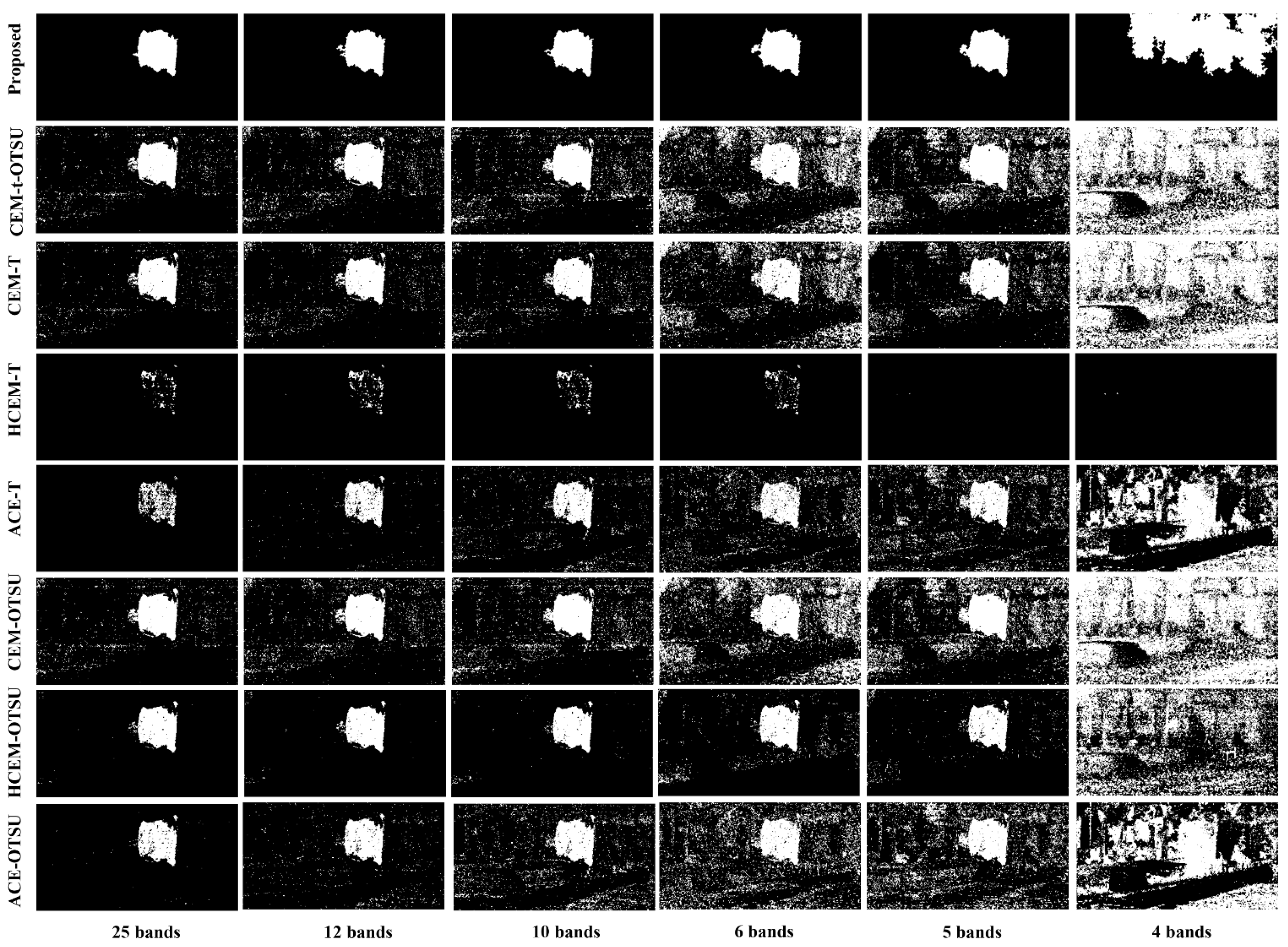
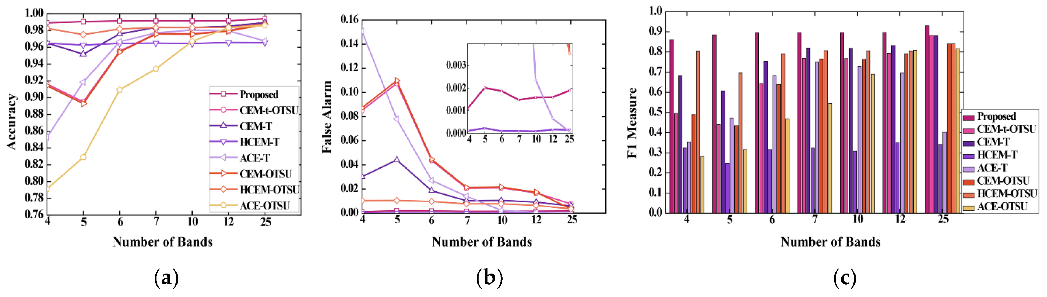
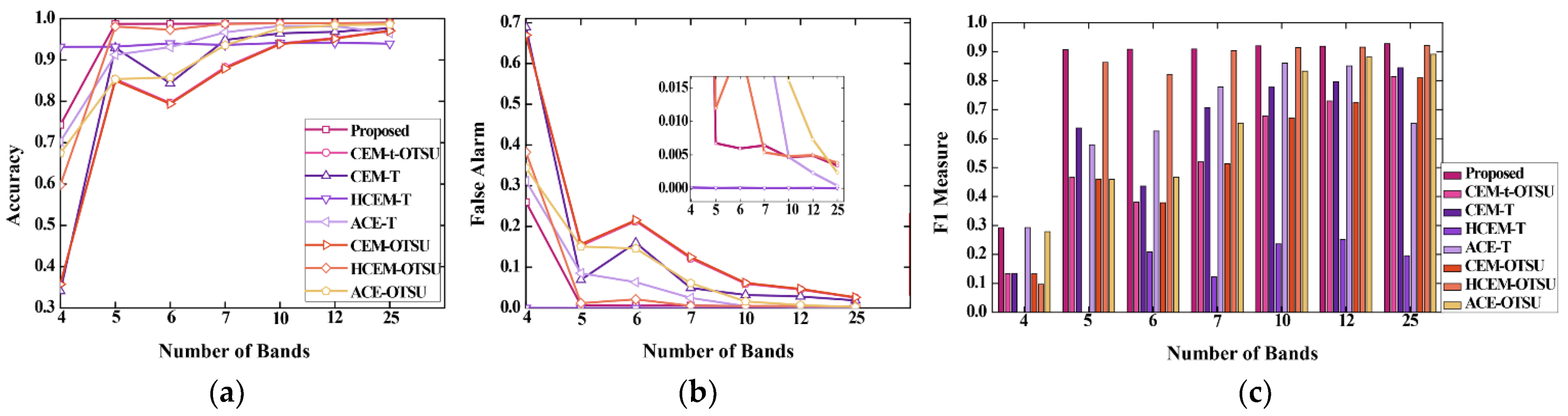
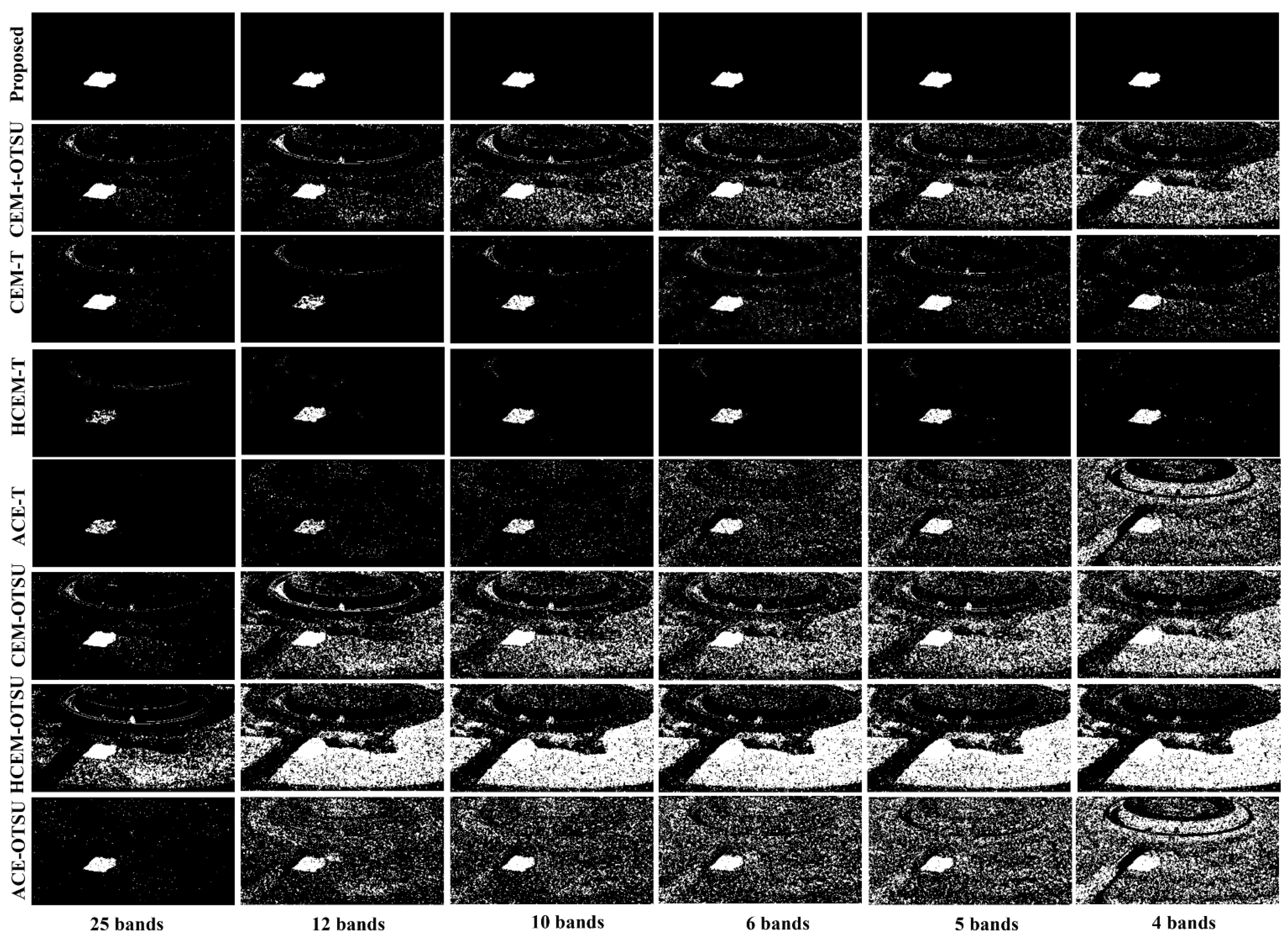
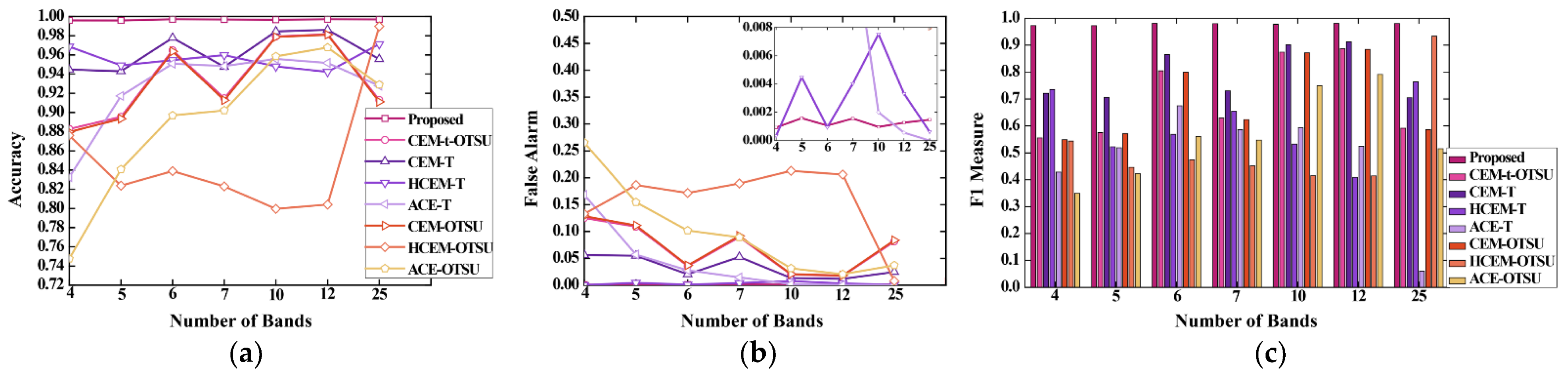
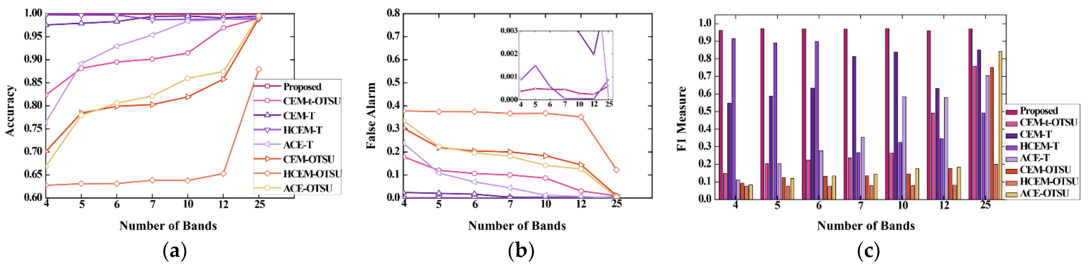
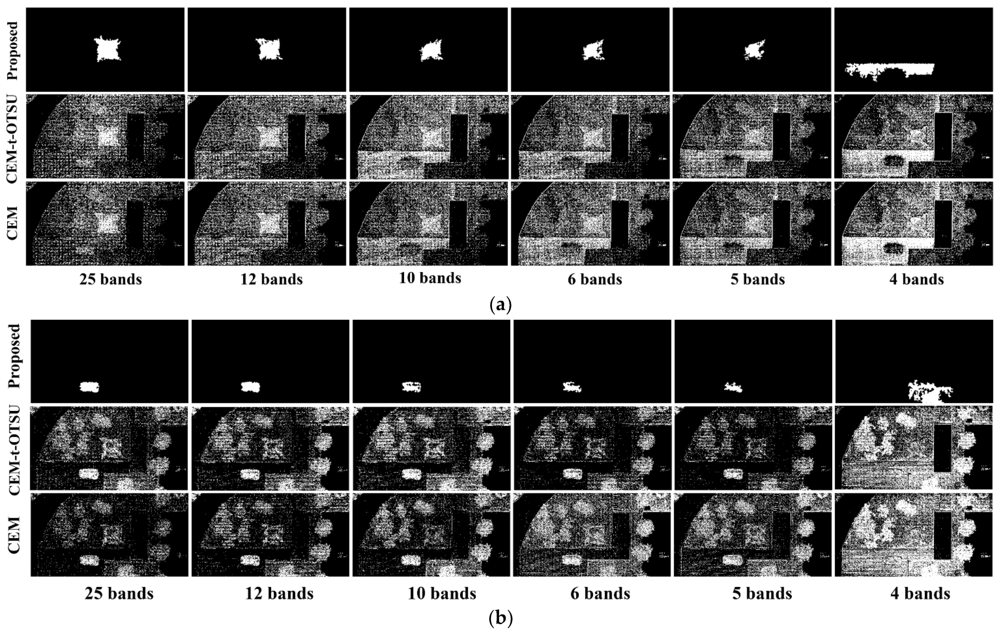
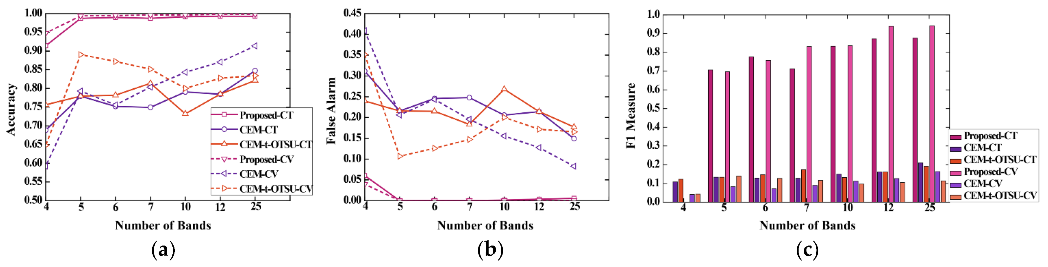
3.2. Results of the Band Selection

Data redundancy is a critical issue in MSI. To address this problem, a band selection algorithm named OCF is introduced. The OCF [14] constructs an optimal cluster structure on HSI, and the discriminative information between the bands is evaluated based on a cluster ranking strategy for the achieved structure to determine the optimal band combination. Figure 4 shows the flow chart of the OCF algorithm.
As shown in Table 2, we determine a series of subsets of bands, where the number of bands ranged from 4 to 25. In each band subset, the specific bands are selected by ranking the occurrence frequency of the characteristic bands. The above characteristic bands are obtained by applying the OCF algorithm to the abundant data of the first three urban scenarios.

3.3. Compared Methods

The effectiveness of the proposed methods is evaluated by comparing the proposed algorithm with six commonly applied algorithms, namely ACE-T, CEM-T, HCEM-T, ACE-OTSU, CEM-OTSU, and HCEM-OTSU. The ACE-T, CEM-T, and HCEM-T are the combination of the ACE algorithm [6], the CEM algorithm [10], the HCEM algorithm [3], and a fixed threshold T, respectively. In addition, ACE-OTSU, CEM-OTSU, and HCEM-OTSU are the combinations of OTSU [29] and the three previously mentioned algorithms, respectively. To analyze whether the performance improvement of the algorithm is brought by the t-OTSU algorithm or the ORE algorithm, we also combine CEM with t-OTSU as an additional comparison. In the HCEM detector, the CEM detector is used as a basic detector in each layer. The spectrum of a target is iteratively updated based on the output of the upper layer. Meanwhile, the parameter t of the t-OTSU algorithm is set to 0.3, while the fixed threshold T is set to 0.5. The remaining parameters of HCEM are kept as the default. It should be noted that the input spectrums we use in the algorithms are obtained by the snapshot multispectral camera. Due to the diversity of colors of two camouflaged nets, we use the average spectrums of multiple regions on their surfaces as input spectrums of the algorithms.
The data were processed with the Matlab 2018 under a win 10 system on a desktop computer with an i5 six-core CPU and 16GB memory.

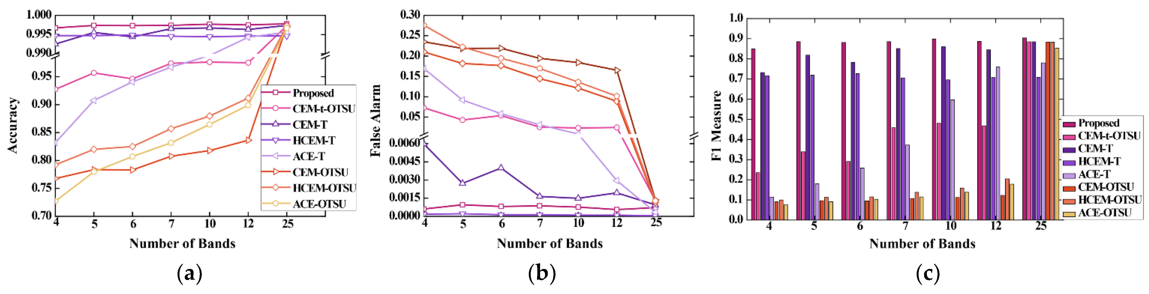
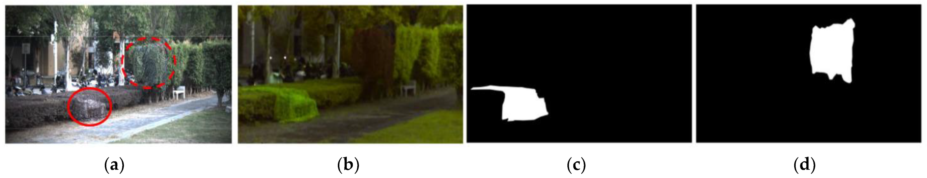
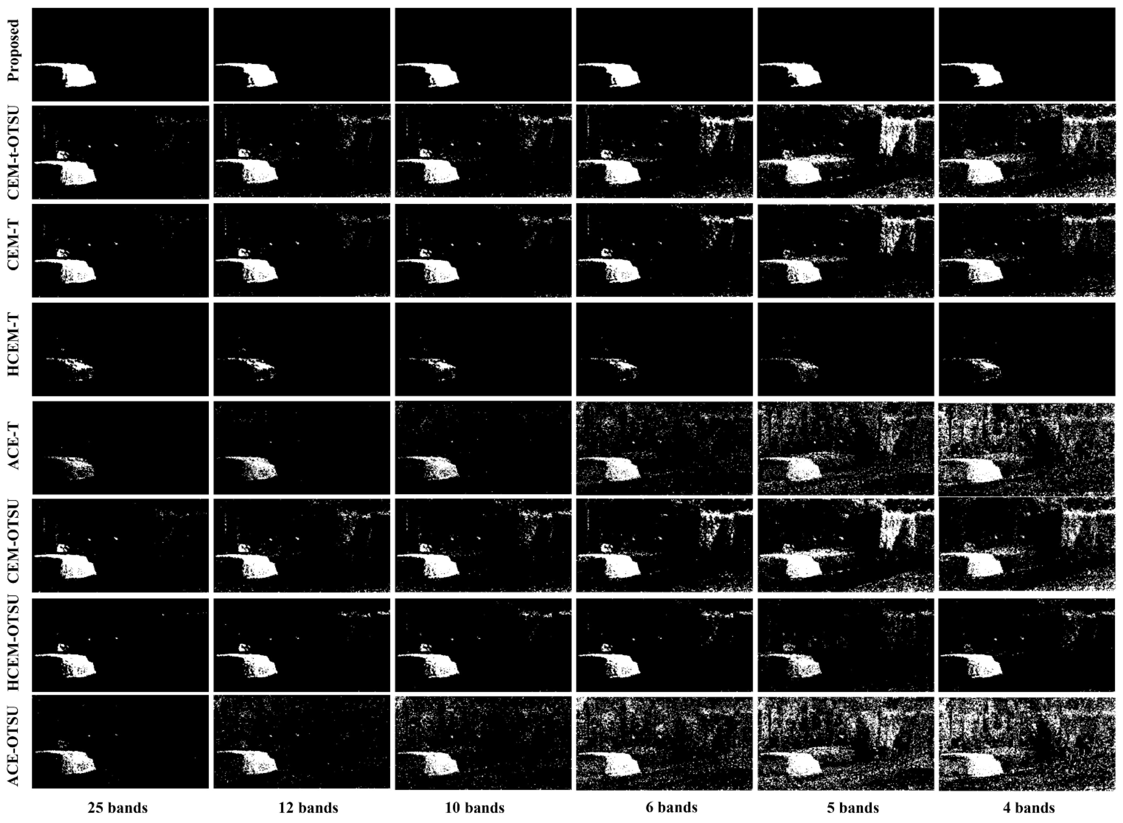
3.4. Experimental Results with the Lawn Scene

As shown in Figure 5a, the ASRC-net and the AIRC-net are spread on a lawn with sufficient light. The false-color image (Figure 5b) shows that the AIRC-net can be easily identified from the background of the lawn. On the other hand, the special design of the ASRC-net makes it barely distinguishes from the lawn. The reference images of the ASRC-net and AIRC-net are shown in Figure 5c,d, respectively.
The detection results of the ASRC-net and AIRC-net are exhibited in Figure 6 and Figure 7, respectively. It is notable that as the number of bands decreases, the misjudged areas all increase with all five comparison algorithms except HCEM-T. With inadequate band numbers, the contour of the target is unclear with the algorithm of HCEM-T, which affects our judgment of the target area. As discussed earlier, the performance of the OTSU algorithm is influenced by the target size [30]. When the target is relatively small, a large number of background pixels are misclassified as the target, which was the reason for a large number of misjudged areas in the detection results of HCEM-OTSU, CEM-OTSU, and ACE-OTSU algorithms. However, the improved t-OTSU algorithm can avoid this phenomenon well, as can be seen from the ASRC-net detection results of CEM-t-OTSU (Figure 6). It is noteworthy that the performance of the recently proposed HCEM is even worse than the original CEM algorithm. The main reason is that based on the principle of HCEM, the reweighted target spectrum in each layer gradually deviates from the real target spectrum. It is possible to exhibit better performance when the target spectra occupy a larger proportion of data [1].
Wang [10] et al. discussed that the decrease in spectral resolution caused by the reduction of bands has a serious impact on the performance of comparison methods. Figure 8 (ASRC-net) and Figure 9 (AIRC-net) compare the A C , F a , and F 1 corresponding to the detection results of the seven algorithms, respectively. As compared with several other algorithms, the proposed algorithm maintains relatively high target contour integrity due to the combination of the improved t-OTSU algorithm and the ORE algorithm. When the number of bands reduces from 25 to 4, the A C values corresponding to the ASRC-net and AIRC-net are above 0.996 and 0.995, respectively, which are higher than the compared algorithms. The F a values corresponding to the proposed algorithm are below 0.0015, which is slightly higher than the HCEM-T algorithm. The F 1 value considers both the precision and the recall, which reflects the performance of the camouflaged target detection algorithm more comprehensively [33]. When the number of bands is above 5, the F 1 value corresponding to the ASRC-net result obtained by the proposed algorithm stays above 0.9. It has to be pointed out that the highest value corresponding to other algorithms is only 0.81 (CEM-T), as presented in Figure 8c. When the proposed algorithm is applied to detect AIRC-net in MSIs with four bands, the result F 1 is around 0.91. The specific analysis of detection results and quantitative metrics shows that in a simple urban background (Lawn) with sufficient light (light intensity: 19,618 lux), the proposed method shows good performance and robustness in detecting different camouflaged targets.

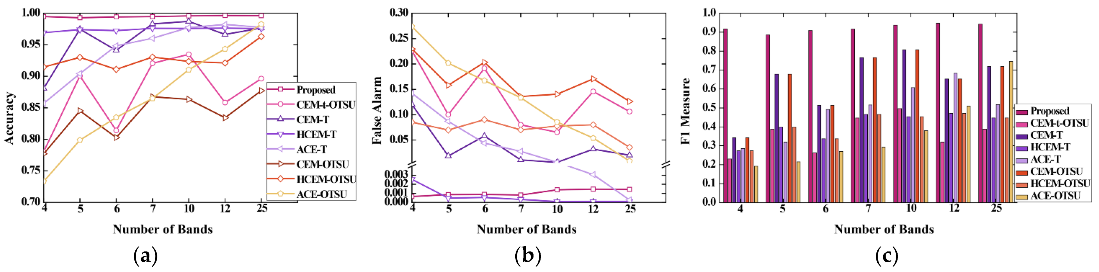
3.5. Experimental Results in the BT Scene

As compared to the Lawn scene, the background of the BT scene in the city is more complicated, as it includes bushes (with both brown and green color), trees, lawn, and building. The positions of the two camouflaged nets are marked in Figure 10a. In order to distinguish the targets from the background, a corresponding false-color image is provided in Figure 10b. The reference images of camouflaged targets are shown in Figure 10c,d, respectively.
Figure 11 (ASRC-net) and Figure 12 (AIRC-net) show that the performance of our algorithm is barely affected in the BT scenes in insufficient light conditions, and complete target contours are obtained in the MSI of different bands. However, we notice that when the number of bands is reduced to four, the detection results of the AIRC-net are greatly affected. A possible reason is that imaging noise caused by poor lighting conditions aggravated the mismatch between the prior spectrum and the in-scene signature, causing a degradation in the performance of the algorithms [5,7]. In this experimental scenario, we find out that the optimization of the t-OTSU algorithm is not obvious. This is because the targets account for a large proportion and the difference between the thresholds obtained by the t-OTSU algorithm and those obtained by the OTSU algorithm is small.
As can be seen in the comparison of evaluation metrics in Figure 13 (ASRC-net) and Figure 14 (AIRC-net), the performance of several compared algorithms (CEM-T, HCEM-T, CEM-OTSU, and HCEM-OTSU) are relatively stable when the number of bands ranges from seven to 25. The CEM-t-OTSU and CEM-OTSU algorithms also exhibit very similar performance due to the similarity of the thresholds. However, the ACE algorithm is more sensitive to the change of bands number. On the contrary, our algorithm maintains a stable performance, as the A C and F 1 remain above 0.99 and 0.85, respectively, and the F a remains stable around 0.0015. By analyzing the results in the BT scene, our algorithm can well overcome the impact of imaging noise caused by the insufficient light intensity (1370 lux).

3.6. Experimental Results in the BF Scene

To explore the effectiveness of the proposed algorithm in detecting the camouflaged targets at different distances, we use lenses of 16 mm and 35 mm focal lengths to simulate distance variations in the urban BF scene containing people, roads, fountains, and green and brown bushes, in which the ASRC-net is set as a target. As compared with the image acquired by a 16 mm focal length lens shown in Figure 15a, the target occupies a much larger proportion in the image acquired by a 35 mm focal length lens shown in Figure 15c. In addition, the reference images of the target for different focal lengths are shown in Figure 15b,d.
The detection results of different methods are shown in Figure 16 (35 mm) and Figure 17 (16 mm), respectively. The results show that the complete target contours in MSI of different focal lengths are detected by using the proposed method. However, since the OTSU algorithm is very sensitive to the target size [23], a large number of misjudged areas are generated by CEM-OTSU, ACE-OTSU, and HCEM-OTSU. The situation is even worse with a 16 mm focal length than with a 35 mm focal length. There is no doubt that the optimization effect of the t-OTSU algorithm is more prominent in images at 16 mm focal length than at 35 mm focal length.
The performance of the eight methods at different focal lengths are shown in Figure 18 (35 mm) and Figure 19 (16 mm), respectively. The robustness of the proposed method is shown by comparing Figure 18 and Figure 19. The A C is stable and above 0.995, F a is around 0.001, while F 1 stays above 0.93. In the MSIs of the 35 mm focal length, the overall performance of several comparison methods fluctuated greatly with the decrease in bands. However, in the images of the 16 mm focal length, the overall performance of several comparison methods showed a monotonically decreasing trend without fluctuations, which indicated that these methods were more influenced by the imaging distance. It is noteworthy that there is a great improvement in the performance of HCEM-T when the number of bands is reduced from 25 to 12. We also see similar phenomena in the work of other researchers. For instance, Christian [35] pointed out that the principal component analysis (PCA) method used fewer bands, but still obtaining better performance than using all bands. It is also noted in the literature [36] that the improved sparse subspace clustering (ISSC) and linear prediction (LP) methods also used fewer bands and yet obtained higher accuracy than using all bands. However, we may need additional theoretical studies to fully explain the above observations.
In the BF scene, the proposed method detects the complete target contour at different distances, which demonstrates the robustness of the proposed method to variations of distance.

3.7. Experimental Results in the UAV Scene

To verify the versatility of our proposed method, we used a UAV-mounted snapshot multispectral camera to capture two camouflaged targets in a complex scene at an altitude of 50 m. As shown in Figure 20a, the scene contains roads, trees, grass, a pool, and other objects. The camouflaged tent (CT) is used to simulate illegal buildings, and the vehicle covered with the camouflaged net is used to simulate camouflaged vehicles (CV). These two targets are covered by the AIRC-net. In addition, the reference images of the two targets are shown in Figure 20c,d. The previous experiments prove that the performance of the CEM algorithm is better than the other two comparison algorithms (ACE and HCEM), so we only take the CEM algorithm as a comparison in this scenario. It should be noted that in this scenario, the CEM algorithm is combined with a fixed threshold of 0.7, and the value of the parameter t of the t-OTSU algorithm is set to 0.65.
The detection results of the two targets are shown in Figure 21a,b, respectively. Compared with the previous scenes, such as the Lawn scene and the BT scene, the performance of the CEM algorithm significantly declines in this scenario, and it is difficult to identify the position of the camouflaged targets. In our method, the completeness of the contour decreases as the bands decrease, but the position of the camouflaged targets can still be easily distinguished. When the number of bands reduces to four, the performance of the proposed algorithm degrades greatly.
Figure 22 shows that the performance of the proposed method is significantly better than the CEM algorithm. In addition, the advantages of the t-OTSU algorithm gradually become apparent as the number of bands decreases. Interestingly, the proposed method has better detection results for the CV target than the CT targets. We analyze that the reason may lie in the fact that the CT target is propped up, with a less flat surface and more folds, which leads to an increase in spectral variability that reduces the target detection performance [7]. The CT target surface is flatter and more regular in shape, which is more favorable for our algorithm. When the number of bands is reduced to four, the detection accuracy of the proposed algorithm decreases significantly, and we consider that it may be caused by the unsuitability of the selected bands. Since these four common bands are selected based on the previous experimental scenarios, the UAV scene varies considerably relative to the previous scenes, and other more representative band subsets exist in the UAV scene. In general, the proposed algorithm is more robust than other algorithms, showing good detection performance in this complex UAV scene.
In the Supplementary Materials, we also use the proposed algorithm to detect the targets one by one in the same scene. The comparison with other algorithms further illustrates the effectiveness and robustness of our algorithm.

3.8. Parameter Analysis

Regarding the choice of threshold, the threshold is usually set larger to improve the accuracy of target detection in related applications of HSI [3]. However, as demonstrated in the experiment, setting a larger fixed threshold in the MSI will lead to an incomplete target contour, and the OTSU algorithm is greatly affected by the size of the target. In the scene where the target is relatively small, the target segmentation accuracy of the OTSU algorithm is worse. To address the problem, based on the analysis of the contour of the camouflaged target, we proposed the t-OTSU algorithm and the ORE algorithm. As an important parameter in the proposed t-OTSU algorithm, t greatly affects the performance and robustness of the proposed method. Therefore, in order to determine the appropriate value of t , experiments with different values of t are conducted to obtain the mean values of evaluation metrics for several scenes.
As shown in Table 3, the values of A C , F a , and F 1 of the proposed method show a decreasing trend. This indicates that the performance of the proposed algorithm decreases as the value of t increases from 0.3 to 0.6. When t is set to 0.2 and 0.3, there is an unobvious change in the performance of the algorithm. In order to improve the accuracy of target detection in most scenes, the parameter t is set to 0.3.

4. Discussion

In our experiments, the band selection method was utilized to obtain MSI containing only a few bands and thus reduce the computational effort. Experimental results show that as the number of bands decreases, the performance of the comparison algorithms also declines [37]. Interestingly, we noticed that different methods show different sensitivities to changes in the number of bands. The ACE algorithm is the most sensitive in that its performance declines the most as the number of bands decreases. The reduction of bands also leads to an improvement in the performance of specific algorithms, which means that more but redundant spectral bands may be more harmful than fewer but non-redundant bands [21].
In addition, an important influencing factor in the practical applications of spectral image target detection is the lighting conditions. Experiments prove that the combination of a few bands and poor illumination conditions is a disaster for the target detection applications in MSI. The performance of the recently proposed HCEM algorithm is even worse than the original CEM algorithm. The main reason may be that the reweighted target spectrum in each layer gradually deviates from the real target spectrum due to the interference of the background noise caused by the poor lighting condition. It also suggests that the algorithms that perform well in the laboratory may not necessarily be superior in real-world applications [5].
Combined with the subsequent UAV experiments, it can be found that the proposed algorithm has a better detection capability for the camouflaged targets with regular shapes and flat surfaces. For irregularly shaped targets, the spectral inconsistency brought by their surface shadows or folds weakens the performance of the algorithms.
At the same time, we compare the UAV experiment with the results of the previous three experiments and find out that the performance of the algorithm slightly declines. The reason is that the UAV scenario is more complex than the other three experimental scenarios, and the original waveband subset is not fully suitable for this scenario. This also shows that in order to achieve excellent target detection with fewer bands, it is necessary to select different subsets of bands for different scenarios [13,14].
The flow chart of the proposed algorithm (Figure 1) shows that the CEM detector plays a key role in distinguishing the camouflaged nets and vegetation, and the ORE algorithm plays a critical role in obtaining an accurate and complete target contour. Although the results show that the performance of CEM-T is better than that of CEM-t-OTSU in simple scenarios, the t-OTSU algorithm showed its advantages when the scene becomes more complicated, such as the last UAV scene. In summary, the t-OTSU algorithm is mainly used to adaptively segment out the complete target contour, contributing to the robustness of the proposed algorithm in different scenarios. Meanwhile, the ORE algorithm is used to accurately obtain the target region, playing a significant role in improving the performance of our algorithm. For the application of camouflaged targets detection, these two algorithms are both indispensable in our study. In general, this algorithm can overcome influencing factors such as low spectral resolution and poor lighting conditions and is more suitable for fast and high-precision detection of unoccluded targets within 100 m. However, when the light intensity in the scene is lower than 800 lux, the detection performance of our algorithm is significantly reduced. Meanwhile, it should be noted that this algorithm is not suitable for the detection of unknown camouflaged targets, which is also a common problem of algorithms such as CEM and HCEM.

5. Conclusions

In this work, we introduce a rapid and accurate camouflaged targets detection method by using a snapshot multispectral camera. Firstly, we screen several general-purpose bands used for the detection of the camouflaged targets based on snapshot multispectral imaging technology and band selection methods. Additionally, a method based on the constrained energy minimization (CEM) algorithm and improved OTSU algorithm is proposed to adaptively segment the camouflaged target region in MSIs. The CEM detector is used to obtain the initial detection results. Then, the improved OTSU algorithm adds a minimum threshold t to segment the target region. In order to eliminate the interference of misjudged areas and obtain a complete camouflaged target contour, the object region extraction (ORE) algorithm is proposed. The experimental results of two different targets in four typical urban scenes show that our proposed algorithms achieve better performance of camouflaged target detection using only four bands as compared to other algorithms that using all 25 multispectral bands, which is of great importance in practical applications. The proposed method achieves A C over 0.99, F a while remains under 0.002, and F 1 is over 0.9. In addition, the proposed method also exhibits the best robustness in experiments using multiple focal length lenses to simulate a variation in imaging distances.
A snapshot multispectral camera is a relatively new imaging device in recent years. It is extremely limited to the select matched spatial resolution and band range of a snapshot multispectral camera. In the future, the snapshot camera could be customized so that it is more suitable for target detection according to the proposed algorithm. Meanwhile, we will build a data set of camouflaged targets based on the snapshot multispectral camera, using deep learning-based algorithms to detect unknown camouflaged targets in complex scenes under long-distance, poor lighting conditions.

Supplementary Materials

The following are available online at https://www.mdpi.com/article/10.3390/rs13193949/s1, Figure S1: Detection results of the two camouflaged nets in different scenarios with bands ranging from 4 to 25. (a) The detection results of two targets in the Lawn scene. (b) The detection results of two targets in the BT scene. (c) The detection results of two targets in the UAV scene, Figure S2: The quantitative comparison of the detection results of two targets in different scenes. (a) The curves of AC using different methods for the two targets. (b) The curves of Fa using different methods for the two targets. (c) The histograms of F1 using different methods for the two targets.

Author Contributions

Conceptualization, Y.S., F.H., J.L. and S.W.; methodology, J.L.; software, J.L.; investigation, J.L., W.L., L.C.; formal analysis, J.L., W.L. and S.W.; writing—original draft preparation, J.L. and Y.S.; writing—review and editing, Y.S., J.L., F.H., S.W. All authors have read and agreed to the published version of the manuscript.

Funding

This work was supported by the National Natural Science Foundation of China (62005049); Natural Science Foundation of Fujian Province (2020J01451); Education and Scientific Research Foundation for Young Teachers in Fujian Province (JAT190003); and Fuzhou University Research Project (GXRC-19052).

Institutional Review Board Statement

Not applicable.

Informed Consent Statement

Not applicable.

Data Availability Statement

A formal dataset was not completed in the paper. Data used in the figures is available upon request.

Conflicts of Interest

The authors declare no conflict of interest.

References

  1. Zhao, R.; Shi, Z.; Zou, Z.; Zhang, Z. Ensemble-based cascaded constrained energy minimization for hyperspectral target detection. Remote Sens. 2019, 11, 1310. [Google Scholar] [CrossRef] [Green Version]
  2. Bárta, V.; Racek, F. Hyperspectral discrimination ofcamouflaged target. In Proceedings of the SPIE 10432: SPIE Security + Defence: Target and Background Signatures III, Warsaw, Poland, 11–12 September 2017; p. 1043207. [Google Scholar]
  3. Zou, Z.; Shi, Z. Hierarchical Suppression Method for Hyperspectral Target Detection. IEEE Trans. Geosci. Remote Sens. 2016, 54, 330–342. [Google Scholar] [CrossRef]
  4. Manolakis, D.; Marden, D.; Shaw, G.A. Hyperspectral image processing for automatic target detection applications. Linc. Lab. J. 2003, 14, 79–116. [Google Scholar]
  5. Manolakis, D.; Truslow, E.; Pieper, M.; Cooley, T.; Brueggeman, M. Detection algorithms in hyperspectral imaging systems: An overview of practical algorithms. IEEE Signal Process. Mag. 2013, 31, 24–33. [Google Scholar] [CrossRef]
  6. Manolakis, D.; Lockwood, R.; Cooley, T.; Jacobson, J. Is there a best hyperspectral detection algorithm? In Proceedings of the SPIE 7334: Algorithms and Technologies for Multispectral, Hyperspectral, and Ultraspectral Imagery XV, Orlando, FL, USA, 13–16 April 2009; p. 733402. [Google Scholar]
  7. Manolakis, D.; Shaw, G. Detection algorithms for hyperspectral imaging applications. IEEE Signal Process. Mag. 2002, 19, 29–43. [Google Scholar] [CrossRef]
  8. Yan, Q.; Li, H.; Wu, Y.; Zhang, X.; Wang, S.; Zhang, Q. Camouflage target detection based on short-wave infrared hyperspectral images. In Proceedings of the SPIE 11023, The Fifth Symposium on Novel Optoelectronic Detection Technology and Application, Xi’an, China, 12 March 2019; p. 110232M. [Google Scholar]
  9. Shi, G.; Li, X.; Huang, B.; Hua, W.; Guo, T.; Liu, X. Camouflage target reconnaissance based on hyperspectral imaging technology. In Proceedings of the 2015 International Conference on Optical Instruments and Technology: Optoelectronic Imaging and Processing Technology, Beijing, China, 5 August 2015. [Google Scholar]
  10. Farrand, W.H.; Harsanyi, J.C. Mapping the distribution of mine tailings in the Coeur d’Alene River Valley, Idaho, through the use of a constrained energy minimization technique. Remote Sens. Environ. 1997, 59, 64–76. [Google Scholar] [CrossRef]
  11. Kumar, V.; Ghosh, J.K. Camouflage Detection Using MWIR Hyperspectral Images. J. Indian Soc. Remote Sens. 2016, 45, 139–145. [Google Scholar] [CrossRef]
  12. Cao, X.; Yue, T.; Lin, X.; Lin, S.; Yuan, X.; Dai, Q.; Carin, L.; Brady, D.J. Computational Snapshot Multispectral Cameras Toward dynamic capture of the spectral world. IEEE Signal Process. Mag. 2016, 33, 95–108. [Google Scholar] [CrossRef]
  13. Karlholm, J.; Renhorn, I. Wavelength band selection method for multispectral target detection. Appl. Opt. 2002, 41, 6786–6795. [Google Scholar] [CrossRef]
  14. Wang, Q.; Zhang, F.; Li, X. Optimal Clustering Framework for Hyperspectral Band Selection. IEEE Geosci. Remote Sens. Mag. 2018, 10, 5910–5922. [Google Scholar] [CrossRef] [Green Version]
  15. Gong, M.; Zhang, M.; Yuan, Y. Unsupervised Band Selection Based on Evolutionary Multiobjective Optimization for Hyperspectral Images. IEEE Trans. Geosci. Remote Sens. 2016, 54, 544–557. [Google Scholar] [CrossRef]
  16. Wei, X.; Zhu, W.; Liao, B.; Cai, L. Scalable One-Pass Self-Representation Learning for Hyperspectral Band Selection. IEEE Trans. Geosci. Remote Sens. 2019, 57, 4360–4374. [Google Scholar] [CrossRef]
  17. Dalla Mura, M.; Atli Benediktsson, J.; Waske, B.; Bruzzone, L. Extended profiles with morphological attribute filters for the analysis of hyperspectral data. Int. J. Remote Sens. 2010, 31, 5975–5991. [Google Scholar] [CrossRef]
  18. Benediktsson, J.A.; Palmason, J.A.; Sveinsson, J.R. Classification of hyperspectral data from urban areas based on extended morphological profiles. IEEE Trans. Geosci. Remote Sens. 2005, 43, 480–491. [Google Scholar] [CrossRef]
  19. Benediktsson, J.A.; Pesaresi, M.; Amason, K. Classification and feature extraction for remote sensing images from urban areas based on morphological transformations. IEEE Trans. Geosci. Remote Sens. 2003, 41, 1940–1949. [Google Scholar] [CrossRef] [Green Version]
  20. Fauvel, M.; Benediktsson, J.A.; Chanussot, J.; Sveinsson, J.R. Spectral and Spatial Classification of Hyperspectral Data Using SVMs and Morphological Profiles. IEEE Trans. Geosci. Remote Sens. 2008, 46, 3804–3814. [Google Scholar] [CrossRef] [Green Version]
  21. Kwan, C.; Gribben, D.; Ayhan, B.; Bernabe, S.; Plaza, A.; Selva, M. Improving Land Cover Classification Using Extended Multi-Attribute Profiles (EMAP) Enhanced Color, Near Infrared, and LiDAR Data. Remote Sens. 2020, 12, 1392. [Google Scholar] [CrossRef]
  22. Kwan, C.; Ayhan, B.; Budavari, B.; Lu, Y.; Perez, D.; Li, J.; Bernabe, S.; Plaza, A. Deep Learning for Land Cover Classification Using Only a Few Bands. Remote Sens. 2020, 12, 2000. [Google Scholar] [CrossRef]
  23. Zhang, C.; Cheng, H.; Chen, C.; Zheng, W. The development of hyperspectral remote sensing and its threat to military equipment. Electro-Opt. Technol. Appl. 2008, 23, 10–12. [Google Scholar]
  24. Liu, K.; Shun, X.; Zhao, Z.; Liang, J.; Wang, S. Hyperspectral imaging detection method for ground target camouflage features. J. PLA Univ. Sci. Technol. (Nat. Sci. Ed.) 2005, 6, 166–169. [Google Scholar]
  25. Tian, Y.; Jin, W.; Zhao, Z.; Dong, S.; Jin, B. Research on UV detection technology of snow camouflage materials based on reflection spectra and images. Infrared Technol. 2017, 39, 469–474. [Google Scholar]
  26. Bao, J.; Bawendi, M.G. A colloidal quantum dot spectrometer. Nature 2015, 523, 67–70. [Google Scholar] [CrossRef]
  27. Jia, J.; Barnard, K.J.; Hirakawa, K. Fourier spectral filter array for optimal multispectral imaging. IEEE Trans. Image Process. 2016, 25, 1530–1543. [Google Scholar] [CrossRef] [PubMed]
  28. Geelen, B.; Carolina, B.; Gonzalez, P.; Tack, N.; Lambrechts, A. A tiny, VIS-NIR snapshot multispectral camera. Proc. SPIE—Int. Soc. Opt. Eng. 2015, 9374. [Google Scholar] [CrossRef]
  29. Otsu, N. A threshold selection method from gray-level histograms. IEEE Trans. Syst. Man Cybern. 1979, 9, 62–66. [Google Scholar] [CrossRef] [Green Version]
  30. Zhang, J.; Hu, J. Image segmentation based on 2D Otsu method with histogram analysis. In Proceedings of the 2008 International Conference on Computer Science and Software Engineering, Wuhan, China, 12–14 December 2008; pp. 105–108. [Google Scholar]
  31. Meng, F.J.; Song, M.; Guo, B.L.; Shi, R.X.; Shan, D.L. Image fusion based on object region detection and Non-Subsampled Contourlet Transform. Comput. Electr. Eng. 2017, 62, 375–383. [Google Scholar] [CrossRef]
  32. Gonzalez, R.C.; Woods, R.E. Digital Image Processing, 3rd ed.; Prentice-Hall, Inc.: Upper Saddle Rive, NJ, USA, 2007. [Google Scholar]
  33. Ma, L.; Jia, Z.; Yu, Y.; Yang, J.; Kasabov, N.K. Multi-Spectral Image Change Detection Based on Band Selection and Single-Band Iterative Weighting. IEEE Access 2019, 7, 27948–27956. [Google Scholar] [CrossRef]
  34. Xue, B.; Yu, C.; Wang, Y.; Song, M.; Li, S.; Wang, L.; Chen, H.; Chang, C. A Subpixel Target Detection Approach to Hyperspectral Image Classification. IEEE Trans. Geosci. Remote Sens. 2017, 55, 5093–5114. [Google Scholar] [CrossRef]
  35. Debes, C.; Merentitis, A.; Heremans, R.; Hahn, J.; Frangiadakis, N.; van Kasteren, T.; Liao, W.; Bellens, R.; Pižurica, A.; Gautama, S. Hyperspectral and LiDAR data fusion: Outcome of the 2013 GRSS data fusion contest. IEEE J. Sel. Top. Appl. Earth Obs. Remote Sens. 2014, 7, 2405–2418. [Google Scholar] [CrossRef]
  36. Sun, W.; Du, Q. Hyperspectral band selection: A review. IEEE Geosci. Remote Sens. Mag. 2019, 7, 118–139. [Google Scholar] [CrossRef]
  37. Geng, X.; Ji, L.; Sun, K.; Zhao, Y. CEM: More Bands, Better Performance. IEEE Geosci. Remote Sens. Lett. 2014, 11, 1876–1880. [Google Scholar] [CrossRef]
Figure 1. The flow chart of the proposed camouflaged target detection method.
Remotesensing 13 03949 g001
Figure 2. (a) The XIMEA camera; (b) The diagram of a 5 × 5 Filter array on the imaging sensor; (c) The ASRC-net; (d) The AIRC-net.
Remotesensing 13 03949 g002
Figure 3. The spectra of different targets and vegetation.
Remotesensing 13 03949 g003
Figure 4. The flow chart of the OCF algorithm (in the figure, each color refers to a cluster of bands). First, the optimal band partition via OCF is based on the given objective function. Then, all the bands are evaluated through an arbitrary ranking method. Finally, the top-rank bands are selected in each cluster.
Remotesensing 13 03949 g004
Figure 5. (a) The visible image of the Lawn scene, where the ASRC-net is circled by the solid line and the AIRC-net is circled by the dashed line; (b) The false-color image of the Lawn scene; (c) The reference image of the ASRC-net; (d) The reference image of the AIRC-net.
Remotesensing 13 03949 g005
Figure 6. The detection results of different methods for the ASRC-net in the Lawn scene with bands ranging from 4 to 25. All the results are normalized to the range [0, 1] for a fair comparison.
Remotesensing 13 03949 g006
Figure 7. The detection results of different methods for the AIRC-net in the Lawn scene with bands ranging from 4 to 25. All the results are normalized to [0, 1] for a fair comparison.
Remotesensing 13 03949 g007
Figure 8. The quantitative comparison of ASRC-net detection results in the Lawn scene. (a) The curves of A C obtained using different methods; (b) The curves of F a obtained using different methods. (c) The histograms of F 1 obtained using different methods.
Remotesensing 13 03949 g008
Figure 9. The quantitative comparison of AIRC-net detection results in the Lawn scene. (a) The curves of A C obtained using different methods; (b) The curves of F a obtained using different methods. (c) The histograms of F 1 obtained using different methods.
Remotesensing 13 03949 g009
Figure 10. (a) The visible image of the BT scene, where the ASRC-net is circled by the solid line and the AIRC-net is circled by the dashed line; (b) The false-color image of the BT scene; (c) The reference image of the ASRC-net; (d) The reference image of the AIRC-net.
Remotesensing 13 03949 g010
Figure 11. The detection results of different methods for the ASRC-net in the BT scene with bands ranging from 4 to 25. All the results are normalized to [0, 1] for a fair comparison.
Remotesensing 13 03949 g011
Figure 12. The detection results of different methods for the AIRC-net in the BT scene with bands ranging from 4 to 25. All the results are normalized to [0, 1] for a fair comparison.
Remotesensing 13 03949 g012
Figure 13. The quantitative comparison of the ASRC-net detection results in the BT scene. (a) The curves of A C obtained using different methods; (b) The curves of F a obtained using different methods. (c) The histograms of F 1 obtained using different methods.
Remotesensing 13 03949 g013
Figure 14. The quantitative comparison of AIRC-net detection results in the BT scene. (a) The curves of A C obtained using different methods; (b) The curves of F a obtained using different methods; (c) The histograms of F 1 obtained using different methods.
Remotesensing 13 03949 g014
Figure 15. (a) The visible image of the BF scene at 35 mm focal length, where the ASRC-net is circled by the solid line; (b) The reference image of the ASRC-net at 35 mm focal length; (c) The visible image of the BF scene at 16 mm focal length, where the ASRC-net is circled by the solid line; (d) The reference image of the ASRC-net at 16 mm focal length.
Remotesensing 13 03949 g015
Figure 16. The detection results of the ASRC-net in the BF scene (35 mm focal length) with bands ranging from 4 to 25. All results are normalized to [0, 1] for a fair comparison.
Remotesensing 13 03949 g016
Figure 17. The detection results of the ASRC-net in the BF scene (16 mm focal length) with bands ranging from 4 to 25. All results are normalized to [0, 1] for a fair comparison.
Remotesensing 13 03949 g017
Figure 18. The quantitative comparison of ASRC-net detection results in the BF scene at 35 mm focal length; (a) The curves of A C obtained using different methods; (b) The curves of F a obtained using different methods; (c) The histograms of F 1 obtained using different methods.
Remotesensing 13 03949 g018
Figure 19. The quantitative comparison of ASRC-net detection results in the BF scene at 16 mm focal length; (a) The curves of A C using different methods; (b) The curves of F a using different methods; (c) The histograms of F 1 using different methods.
Remotesensing 13 03949 g019
Figure 20. (a) The visible image of the UAV scene. The camouflaged tent is circled by the solid line. The camouflaged vehicle is circled by the dashed line; (b) The false-color image of the UAV scene; (c) The reference image of the camouflaged tent; (d) The reference image of the camouflaged vehicle.
Remotesensing 13 03949 g020
Figure 21. The detection results of two targets in the UAV scene with bands ranging from four to 25. (a) The results of camouflaged tent detection with different algorithms. (b) The results of camouflaged vehicle detection with different algorithms. All results are normalized to [0, 1] for a fair comparison.
Remotesensing 13 03949 g021
Figure 22. The quantitative comparison of the detection results of two targets in the UAV scene. (a) The curves of A C using different methods for the two targets. (b) The curves of F a using different methods for the two targets. (c) The histograms of F 1 using different methods for the two targets.
Remotesensing 13 03949 g022
Table 1. The basic parameters of the experiments.
SceneDistance
/m
Focus Length
/mm
FOV
/cm2
Light Intensity
/Lux
Integration Time
/ms
Lawn2335740 × 39319,6180.154
BT2535804 × 42713705
BF20161408 × 74816003
2035644 × 34216003
UAV50163520 × 187018003
Table 2. Subsets of bands in the first three urban scenarios.
Number of BandsThe Wavelength of Selected Bands (nm)
12665/686/710/727/738/751/779/787/850/897/911/949
10665/686/710/738/751/802/841/897/911/949
7665/686/710/738/751/841/897
6665/710/751/766/779/897
5665/710//751/779/841
4665/710/727/751
Table 3. Experimental results with different parameters t . The best results are bolded.
t = 0.2 t = 0.3 t = 0.4 t = 0.5 t = 0.6
SCENE A C ¯ F a ¯ F 1 ¯ A C ¯ F a ¯ F 1 ¯ A C ¯ F a ¯ F 1 ¯ A C ¯ F a ¯ F 1 ¯ A C ¯ F a ¯ F 1 ¯
LAWN0.99700.00170.92120.99700.00160.92220.9970 0.0012 0.9215 0.9957 0.0008 0.8952 0.9919 0.0005 0.8057
BT0.99230.00280.93000.99230.00280.93000.9923 0.0028 0.9300 0.9909 0.0021 0.9080 0.9891 0.0014 0.8863
BF0.99800.00110.97460.99800.00110.97460.9980 0.0011 0.9746 0.9980 0.0010 0.9728 0.9980 0.0009 0.9723
Publisher’s Note: MDPI stays neutral with regard to jurisdictional claims in published maps and institutional affiliations.

