Abstract
Large uncertainty exists in the estimations of greenhouse gases and aerosol emissions from crop residue burning, which could be a key source of uncertainty in quantifying the impact of agricultural fire on regional air quality. In this study, we investigated the crop residue burning emissions and their uncertainty in North China Plain (NCP) using three widely used methods, including statistical-based, burned area-based, and fire radiative power-based methods. The impacts of biomass burning emissions on atmospheric carbon dioxide (CO2) were also examined by using a global chemical transport model (GEOS-Chem) simulation. The crop residue burning emissions were found to be high in June and followed by October, which is the harvest times for the main crops in NCP. The estimates of CO2 emission from crop residue burning exhibits large interannual variation from 2003 to 2019, with rapid growth from 2003 to 2012 and a remarkable decrease from 2013 to 2019, indicating the effects of air quality control plans in recent years. Through Monte Carlo simulation, the uncertainty of each estimation was quantified, ranging from 20% to 70% for CO2 emissions at the regional level. Concerning spatial uncertainty, it was found that the crop residue burning emissions were highly uncertain in small agricultural fire areas with the maximum changes of up to 140%. While in the areas with large agricultural fire, i.e., southern parts of NCP, the coefficient of variation mostly ranged from 30% to 100% at the gridded level. The changes in biomass burning emissions may lead to a change of surface CO2 concentration during the harvest times in NCP by more than 1.0 ppmv. The results of this study highlighted the significance of quantifying the uncertainty of biomass burning emissions in a modeling study, as the variations of crop residue burning emissions could affect the emission-driven increases in CO2 and air pollutants during summertime pollution events by a substantial fraction in this region.
1. Introduction
Crop residue burning, which is a kind of biomass burning, releases significant amounts of combustion products into the atmosphere, including carbon dioxide (CO2), carbon monoxide (CO), methane (CH4), non-methane organic volatile organic compounds (NMVOCs), black carbon (BC), organic carbon (OC), nitrogen oxides (NOx), ammonia (NH3), sulfur dioxide (SO2), and particulate matter (PM). In China, crop residue burning is a common management practice in the agricultural zones during the pre-planting, harvesting, and post-harvesting stages. In other words, the crop residue is the majority of biomass burning in the open in China [1]. Notably, previous studies have indicated that the open crop fires may rapidly degrade the local air quality in harvest seasons and significantly affect the atmospheric chemistry and climate change in eastern China, such as North China and the Yangtze River delta [1,2,3,4,5,6]. Moreover, biomass burning CO2 emissions remain a large source of uncertainty in estimates of global and regional carbon budgets [7].
Considerable efforts have been made to estimate the agricultural residue burning emissions in China [8,9]. Some studies obtained the amounts and distribution of crop residue burning emissions based on the statistical data, such as crop yield, dry matter-to-crop residue ratio, percentage of dry matter burned in the field, combustion efficiency, and emission factors [10,11]. To improve the state of crop residue-burning emissions at the national or regional scale, some studies have estimated the emissions from crop residue burning by using remote sensing data, such as active fire products, burned area (BA) products, and fire radiative power (FRP) products [12,13,14,15,16]. Presently, multiple estimations on crop residue burning emissions in China produced by satellite data exist. For example, Huang et al. developed a crop residue burning emissions inventory for the year 2006 in China by applying a statistical method and then obtained the spatial distribution of crop residue burning emissions based on the fire counts detected by satellite observation [12]. With more accurate time-varying statistical data and locally observed emission factors, Li et al. proposed a historical crop residue burning emission inventory and showed that the emissions of the trace gases, greenhouse gases, and PM have increased by 500% to 775% during the period 1990–2013 in China [17]. Qiu et al. built a high-resolution biomass burning emission inventory in China for the year 2013 based on the Moderate Resolution Imaging Spectroradiometer (MODIS) BA product (MCD64Al), the active fire product (MCD14 ML), and a high-resolution land cover dataset, whilst their results obtained that the emissions from cropland accounted for 60–80% of the total open biomass burning emission over China in 2013 [15]. In addition, Liu et al. used an FRP-based method to estimate fire radiative energy (FRE), then to estimate emissions from crop fire in June over the North China Plain from 2003 to 2014 [14]. Recently, Yin et al. applied the FRP-based approach to calculate emissions of biomass burning in China from 2003 to 2017 and found that crop residue emissions continued to increase during 2003–2015 due to socio-economic development with reduced consumption of crop residues as a residential energy source in rural areas, but dropped by 42% during the period 2015–2016 as strict supervisions were implemented [16].
The abovementioned studies provided an improved understanding of the characteristics of crop residue burning emissions in China. However, there is still a lot of uncertainty regarding the annual crop residue burning emissions in terms of spatiotemporal variation and total amounts, especially on a regional scale [1,12,15,18]. The discrepancies among current studies are largely due to the limitation of different estimated approaches, as the estimations depend strongly on relevant parameters and data sources. For instance, multiple parameters required in the statistical-based method (i.e., residue-to-production ratio, dry matter-to-crop residue ratio, percentage of dry matter burned in the field, combustion efficiency, and emission factors) are obtained mainly from field investigations and statistical records that correspond to the local agricultural practices, which may not be updated in time or be suitable for the whole country [19]. While in the satellite-based approach, the uncertainties might arise from the overlook of small fires due to the low temporal and spatial resolution of the satellite products, or be introduced by the overpass time of the orbiting satellite when converting from FRP to FRE [20], the uncertainties in the input data, such as the combustion factor, and the available fuel loads used in either the modeling or inversion approach may enlarge the differences in emissions estimates [21]. The emission factors, FRP measurements, and FRP parameterization are the major sources of the uncertainty of crop residue-burning emissions as well [14].
Some previous studies underscored the differences among several widely used biomass burning emissions inventories derived from multiple satellite datasets, for instance, the Global Fire Emissions Database (GFED3 and GFED4), the Global Fire Assimilation System (GFAS1.0), the Fire Inventory from NCAR (FINN1.0), and the Global Inventory for Chemistry-Climate studies-GFED4 (G-G), but previous studies have mostly focused on the inventories at continental and global scales [22,23]. Little is known about the similarities and discrepancies among crop residue burning emission inventories based on different methods and the spatial distributions and variations with a long timescale at regional levels due to the highly spatiotemporal variability of crop fires. Some studies have investigated the impacts of biomass burning on particulate matter pollution in China [1,3,4,5,6], which reported that crop residue burning can elevate PM2.5 concentration by 34% and 37% (~40 μg m−3) in the North China Plain and Yangtze River delta, respectively, during summertime pollution episodes. No previous studies, to our knowledge, have examined the impacts of crop residue-burning emissions on atmospheric CO2 concentrations in China.
In this study, we developed three different emissions inventories from crop residue burning in the North China Plain during the period 2003–2019 by using multiple approaches, including the statistical-based, BA-based, and FRP-based approaches. In particular, we aimed to identify the spatial characteristics and seasonal and inter-annual variations of crop residue-burning emissions in the study region through a comparison of the three emissions inventories developed in this study. Additionally, we attempted to highlight the similarities and differences in the geographical patterns, trends, and temporal variation of the three estimations by examining the associated uncertainties in crop residue burning emissions. Special focus was given to the impacts of biomass burning emissions and their uncertainty in atmospheric CO2 simulation, which might be of particular importance to climate and environmental research.
2. Materials and Methods
2.1. Study Area
The NCP—including two province-level municipalities, Beijing and Tianjin, and six provinces, Hebei, Shanxi, Shandong, Henan, Anhui, and Jiangsu (Figure 1)—is one of the city clusters in China with a dense population and the most rapid development of agricultural modernization and a rural economy. Meanwhile, the NCP is also a large contributor of agricultural products in northern China, including wheat and corn, causing large amounts of crop residue to be openly burned. Hence, crop residue burning is the key source of biomass burning emissions in NCP [24], which has been considered as an important factor that influences the air pollution in this region during harvest seasons [1,6].
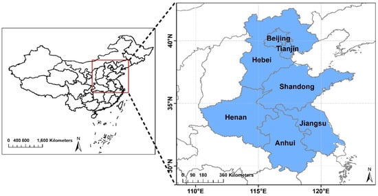
Figure 1.
Location of the study area.
2.2. Methods for Estimating Crop Residue-Burning Emissions
The emissions of CO2, CO, CH4, non-methane hydrocarbon (NMHC), SO2, NH3, NOx, BC, OC, PM2.5, and PM10 from crop fires in NCP were estimated by using statistical-based, BA-based, and FRP-based methods.
2.2.1. Statistical-Based Method
In this method, the emissions from crop fires are estimated by multiplying the total mass of in-field burning crop residues (the product of the crop production, the residue-to-crop ratio, the dry fraction of crop residue, the proportion of crop residues burned in the field, and the combustion factor) and the corresponding emission factor. At a provincial level, the amounts of emissions from crop residues burned in fields were calculated as in Equation (1) [9,25]:
where i and k represent the types of crops and provinces, respectively. is the annual provincial crop production (kg), is the crop-specific residue-to-crop ratio (dry matter). is the dry fraction of crop residue, is the crop-specific proportion of crop residues burned in the field, is the crop-specific combustion factor (Tables S1 and S2), and is the emission factor (g kg−1) (Table S3).
is often seen as a constant value without interannual variation due to the limited availability of investigations. Xu et al. [26] used the MODIS active fire counts to estimate the annual . As a strong relationship between FRP and crop residue burning emissions [27,28], the FRP can be used as a better proxy for spatiotemporal allocation. Similar to Xu et al. [26], we improved the interannual estimations in this work by applying a dynamic annual scale factor () instead of based on the MODIS FRP data:
where j stands for the year. is the crop-specific proportion of crop residues burned in fields for province k in year j. is the sum of FRP that occurred in cropland for province k in year j. is the sum of FRP that occurred in cropland for province k at the base year and is the crop-specific proportion of crop residues burned in fields for province k at the base year, which was collected from the literature (Table S2).
Then, the annual statistical estimations were further interpolated into the monthly emissions in the study domain with a horizontal resolution of 0.05° × 0.05° according to Equation (3).
where m represents the month, represents the gridded crop residue burning for month m, is the monthly gridded scale factor for temporal and spatial allocation, and it can be calculated by using the ratio between the monthly gridded FRP in province i for month m in year j () and the annual total FRP in province i for year j (). is the sum of the estimations () from crop type k in province i for year j.
2.2.2. Burned Area (BA)-Based Method
The amounts of emissions from crop residue burning are generally calculated based on the satellite-derived BA and land cover, together with emission factors, the combustion factor, and estimated fuel loads, as developed by Seiler and Crutzen [29]:
where BA denotes burned area (m2). FL is the available fuel loads, representing the aboveground biomass density in kg (dry matter) m−2, which was set to 0.14 kg dry matter m−2 in this work [30]. CF represents the combustion factor, representing the ratio of actually burned biomass to available biomass; here, the value of 0.86 was applied [18]. EF is the emission factor (g kg−1) (Table S3).
2.2.3. Fire Radiative Power (FRP)-Based Method
This method is based on the assumption that there is a linear relationship between fuel consumption and the total emitted FRE [31]. FRE was estimated by integrating FRP throughout the firing process. As the MODIS FRP data are provided only four times per day (see Section 2.3. for more information), the fire diurnal variations cannot be directly detected by the MODIS sensor [32,33], and the maximum daily fire activity, corresponding to the peak FRP value, would be missed. To reduce the fire event omission error, we assumed that the FRP diurnal cycle of crop residue burning followed a Gaussian distribution and used a modified Gaussian function to parameterize the FRP diurnal cycle following the method of Vermote et al. [34]. The amount of emissions were obtained using Equation (5).
where FRE is the total radiative energy during the fire diurnal cycle (MJ). CR is the associated conversion factor (kg dry matter MJ−1), which is used to convert FRE to combusted biomass. Following the approaches of previous studies in China [14,16,35], an average value (0.411 ± 0.04 kg MJ−1) of Wooster et al. [31,36] and Freeborn et al. [37] was used in this work. EF (g kg−1) is the emission factor (Table S3).
FRPpeak represents the peak of the fire diurnal cycle, b represents the background FRP of the diurnal cycle, σ represents the standard deviation of the curve, t is time, and h is the hour of peak FRP (local time). The parameters b, σ, and h were calculated as a function of Terra/Aqua (T/A) FRP ratios (Equations (6)–(8)) [16,34,38].
where x represents the T/A ratio. Following the method of Liu et al. [14], a parameter ε (ε = 4) was added to modify the FRP peak hour (h) of the diurnal curve, as the original parameterized FRP diurnal cycle could not effectively reproduce the observed FRP temporal variation in the NCP, which was possibly due to the incorrect FRP peak hour. Then, the FRP peak was calculated by using the mean FRP within Aqua daytime observation and the above parameters (Equation (9)).
The emissions from crop residues burning estimated in this work are spatiotemporally allocated with a 0.05° × 0.05° grid size.
2.3. Data Description
The values for the residue-to-production ratios, the dry fraction of crop residue, combustion factors, and provincial proportion of crop residues burned in the field, which were used in the statistical-based method, were compiled from the laboratory measurements and statistical values from previous studies [12,39,40]. More details are shown in Tables S1 and S2. The emission factors for different gaseous and aerosol emissions from crop fires were obtained from previous studies [13,41,42], and listed in Table S3. The provincial-level crop productions were acquired from the China Statistical Yearbook distributed by the National Bureau of Statistics of China (NBSC, available at http://www.stats.gov.cn/english/Statisticaldata/AnnualData/, accessed on 21 July 2021). Due to a lack and deficiency of crop production data for the year 2019, the crop residue-burning emissions were estimated by a statistical-based method for the period of 2003–2018.
The standard quality MODIS Collection 6 Thermal Anomalies/Fire locations product (MCD14ML), with a moderate spatial resolution (1 km) and temporal resolution (daily) for 2003–2019, was used in the FRP-based method. The MCD14ML provided by the Fire Information for Resource Management System (FIRMS) (https://firms.modaps.eosdis.nasa.gov/, accessed on 21 July 2021) is a subset of the standard science quality data processed by the MODIS Fire Team Science Computing Facility at the University of Maryland. The MODIS FRP data are provided four times (10:30 a.m., 10:30 p.m., 01:30 a.m., and 01:30 p.m. at local time) per day by the Terra and Aqua satellites. This product contains information on the geographic location, fire occurrence time, FRP, and other attributes, such as the detection confidence and the inferred hot spot type for each fire point. In this work, the FRP observations were filtered according to the type and confidence parameters provided by the MCD14ML (standard quality) product. Type = 0 denotes the presumed vegetation fire, whereas Types = 1–3 denote active volcano, other static land sources, and offshore fire, respectively [43]. Here, we selected only observations with Type = 0. The detection confidence in the product is intended to help users gauge the quality of individual hotspot/fire pixels. The confidence values range from 0% to 100% and can be used to assign one of the three fire classes (low-confidence fire, nominal-confidence fire, or high-confidence fire) to all fire pixels within the fire mask [43]. To reduce the uncertainty in fire detection, only the fire observations with nominal- and high-confidence were used, and observations with low-confidence were treated as clear, non-fire, land pixels.
The MODIS Collection 6 burned area product (MCD64A1) with a spatial resolution of 500 m and the monthly time resolution for 2003–2019 was used in the BA-based method (https://lpdaac.usgs.gov/products/mcd64a1v006/, accessed on 21 July 2021). The MCD64A1 detected an approximation of burning at a pixel by identifying rapid changes in daily surface reflectance time series data [44]. The validation in previous studies showed that 44% of the MCD64A1 burned pixels were detected on the same day of an active fire, and the detection rate increase to 68% within 2 days, indicating a substantial reduction in the uncertainty of this product in monthly resolution. Overall, the global accuracy, omission error, and commission error of MCD64A1 were 0.97, 0.37, and 0.24, respectively [45].
The MODIS land cover type product (MCD12Q1) with a 500 m horizontal resolution was used to obtain the land cover types in three methods (https://lpdaac.usgs.gov/products/mcd12q1v006/, accessed on 21 July 2021). Here, the types of “cropland” and “Mosaic of crop” in the International Geosphere-Biosphere Programme (IGBP) classification were considered as the cropland. If a fire detected by the MODIS sensor was located in a 500m cropland pixel, it could be recognized as a crop residue burning.
2.4. Method for Quantifying Uncertainties in Crop Residue Burning Emissions
The uncertainties in emissions estimations mainly involve two aspects: (1) the uncertainties induced by the input parameters of each method, and (2) the uncertainties caused by different estimating methods. Here, we used statistical methods to quantify the associated uncertainty of estimates. First, for each method, we used the Monte Carlo simulation to propagate uncertainties in model inputs, then to quantify the uncertainty in each emission estimate. The uncertainties in model inputs for each method were obtained by expert judgment from the literature according to data availability [46]. Second, the uncertainties that arise from different estimated methods were calculated by using statistical parameters, such as the standard deviation (STD) and the coefficient of variation (CV), at the gridded level, which represents the extent of variability.
where is the value of the point in the dataset, is the mean value for the point in the dataset, and is the number of data points.
2.5. Model and Numerical Simulation
The impact of biomass burning emission on atmospheric CO2 concentrations was simulated by using the global chemical transport model (GEOS-Chem) (version 12-01, available at http://acmg.seas.harvard.edu/geos/, accessed on 21 July 2021). The CO2 simulation in GEOS-Chem was developed by Suntharalingam et al. [47], and updated by Nassar et al. [48,49]. The simulation of CO2 in the model is conducted as a separate tracer simulation and can be “tagged” by its source type or region, whose concentrations are determined by atmospheric transport (horizontal and vertical advection and diffusion) and eight types of CO2 emission inventories [49]. This model has been widely utilized to investigate the spatio-temporal variation of CO2 concentration [50,51,52], and the CO2 sources and sinks inversion studies [53,54,55,56]. The abovementioned studies have proven that the model can capture the variations of atmospheric CO2 reasonably well for both seasonal and interannual scales.
The GEOS-Chem CO2 simulation was driven by MERRA-2 meteorological fields [57] for the year 2018 at a 2.5° longitude × 2.0° latitude resolution with 47 vertical layers. The initial fields of the atmospheric CO2 were obtained by GEOS-Chem Unit Tester; then the model was spun up for one year to produce a new restart file for further simulation. The CO2 emission inventories used in this work include the following: the fossil fuel emission from the Open-source Data Inventory for Atmospheric CO2 emissions (ODIAC) with monthly gridded data at 1° × 1° resolution [58]; the biomass burning emissions, including forest wildfire, savanna fires, peat burning, and agricultural residual burning, were obtained from the GFED4 [59]; the biofuel burning emissions from Yevich and Logan, 2013 [60]; the atmosphere-terrestrial ecosystem exchanges were obtained from the Simple Biospheric Model version 3 (Sib3) [61]; the ocean fluxes were taken from Takahashi et al. [62]; the shipping emissions from the International Comprehensive Ocean-Atmosphere Data Set (ICOADS) [63]; the aviation emission from AEIC [64] scaled with global annual CO2 emission totals calculated from the IEA [65]; and the chemical productions from the oxidation of carbon monoxide, methane, and non-methane volatile organic compounds [48].
To investigate the role of biomass burning, atmospheric CO2, as well as the tagged CO2 concentrations from different sources, were simulated by GEOS-Chem using two sets of configurations. The first was designed as the standard simulation with the prescribed emissions and fluxes, as mentioned above. The second was conducted as the comparison simulation, which was similar to the standard simulation but without the biomass burning emissions. Hence, the contribution of biomass burning emissions to surface CO2 concentration was quantified by subtracting the results of the comparison simulation from those of the standard one.
3. Results
3.1. Spatial Distribution of Crop Residue Burning Emissions
For the period 2003–2018, the average annual emissions of CO2, CO, CH4, NMHC, SO2, NH3, NOx, BC, OC, PM2.5, and PM10 at the provincial level in NCP are listed in Table 1. There are notable differences among the three methods at total magnitude. The amount of statistical-based estimation is the highest, while the BA-based estimation is the lowest. The spatial distributions of these pollutants are similar; thus, the seasonal and spatial distributions of CO2 emissions from crop residue burning are used as a representative example. The patterns of crop residue-burning emissions show a reasonable agreement with high emissions concentrated in major cropland regions. As shown in Figure 2, we found that the CO2 emissions obtained from different estimating methods are consistent with the similar features in the spatial distribution, and large emissions were found in the southern part of NCP, where significant amounts of cereal crops exist.

Table 1.
Average annual crop residue-burning emissions (Gg yr−1) in each province during the study period.
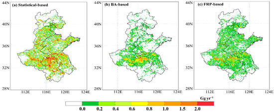
Figure 2.
Spatial distribution of annual CO2 emissions (unit: Gg yr−1) from crop residue burning estimated from the statistical-based method (averaged over 2003–2018), BA-based method (averaged over 2003–2019), and FRP-based method (averaged over 2003–2019), respectively.
However, there are some discrepancies among the distribution of different estimations. For example, it is shown that high crop residue-burning emissions were found in the center and southern area of NCP based on the statistical-based method, while the hot spots of crop fire emissions in southern NCP were not found on the BA-based method. One possible reason for the discrepancies is the differences in the remote sensing-related parameters (i.e., the fire counts or the BA) used in statistical-based and BA-based methods, which show different capabilities of detecting small fires. As in the BA-based method, the spatial distribution of the emissions is dependent on the MODIS BA product. Whilst BA products have been shown to provide high-quality data for the regions where large fires occur, their performance in regions dominated by small fires remains uncertain. As highlighted by previous studies, the MCD64A1 BA product typically fails to detect many of the fires in “small fire dominated” areas, as the changes in landscape spectral reflectance are often not significant enough to be confidently identified by the MCD64A1 BA algorithm in coarse spatial resolution (500 m) [66,67]. However, in the statistical-based method, the estimated emissions are further spatiotemporally allocated through using FRP as a proxy, which might capture much smaller fire-affected areas. Overall, Henan Province and Anhui Province are the largest contributors to the total CO2 emissions from crop fires according to the three methods.
3.2. Temporal Variations of the Emissions and Driving Force
In terms of seasonal variations of CO2 emission from crop residue burning, peak emissions occurred in June, and small peaks were detected in October (Figure 3a), mainly due to the agricultural activities in the NCP region. The open burning of crop residue is a traditional treatment before crop sowing or after crop harvest. In NCP, winter wheat and summer maize rotation are usually important planting patterns. Winter wheat is sown in mid-October and harvested in May–June. The alternative summer maize often grows from June to September and is harvested in October every year. Hence, high crop burning emission mainly occurs in June and October in NCP. Based on all three estimations, the CO2 emissions from crop residue burning in June and October contributed approximately 50–65% of the annual emissions over the study period. The monthly distribution of crop residue-burning emissions in NCP is unlike those in other agricultural regions with different natural and anthropogenic conditions, such as Northeast China, the Chengdu-Chongqing region, and the Pearl River Delta region. For example, the highest crop residue-burning emissions are mainly found in October and April over Northeast China, while in the PRD region, larger emissions are concentrated mainly from November to March [26].
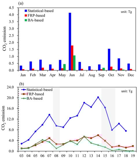
Figure 3.
(a) Seasonal variation of CO2 emission from crop residue burning over the NCP region averaged from 2003 to 2019 based on three methods. (b) Interannual variation of CO2 emission from crop residue burning over the NCP region from 2003 to 2019 based on three methods.
The variations in annual total emissions from crop residue burning in NCP are displayed in Figure 3b. There are some discrepancies in the interannual variations of CO2 emissions from crop residue burning over the period 2003–2019 among the three methods. The interannual variations obtained from the BA method are slightly different from those obtained from the FRP method. The estimations of the FRP method showed a peak in 2014, while the estimations of the BA method exhibited a maximum in 2012. However, the BA estimations agreed well with the FRP estimations in the years with large reductions (i.e., 2008 and 2015). In general, the average annual growth rates of CO2 emission from crop residue burning in the study period are 6.9%, 4.0%, and −12.1% for the statistical-based, FRP-based, and BA-based methods, respectively. The negative growth rate of BA-based estimation, which is opposite to the uptrend of statistical-based and FRP-based estimations, is mainly because of the decrease of crop residue burning emissions (−41.2%) in 2012–2019 that was significantly greater than the increase (13.2%) over 2003–2011.
To examine the effects of rigorous air quality policy since the year 2013, we divided the study period into two distinct stages. It was found that the total crop residue burning emissions derived from the three different methods showed steady increasing trends with annual fluctuations during the period 2003–2012, but sharply decreasing trends during the period 2013–2019 consistently, despite the discrepancies in trends calculated from the three methods for these two periods.
With the economic development and rapid modernization in NCP, the crop production in this region steadily increases during 2003–2018, yielding positive linear trends of 0.5 million tons per year (p < 0.01) and an average annual growth rate of 3.2% (Figure S1). Naturally, the increases in crop yields produce more residues. As the consumption of crop residues for cooking and heating in the rural area decreased sharply from 1992 to 2012 [68], more crop residues were burned in the field, possibly due to the lack of affordable and effective removal mechanisms, which are the main reasons for the increased crop residue burning emissions during the period 2003–2012. Since 2013, a series of stricter pollution-prevention managements were issued nationwide to improve air quality and protect public health rights, i.e., ten measures that were issued by the State Council in the action plan for the prevention and control of air pollution (http://www.gov.cn/zwgk/2013-09/12/content_2486773.htm, accessed on 21 July 2021). Therefore, open crop residue burning is more strictly controlled than before, with the enhanced monitoring of crop residue burning by satellite monitoring. Additionally, the comprehensive utilization rate of crop residues has also been improved through science and technology in recent years. Because of these factors, crop residue-burning emissions have declined significantly since 2013. Note that some severe and effective policies, such as the fire-forbidding policy, were implemented for Beijing and its surrounding provinces to achieve the air quality goals and “blue-sky” during the Beijing Olympic Games 2008, and the Beijing APEC 2015 (http://www.gov.cn/zwgk/2007-06/14/content_648934.htm; http://www.gov.cn/zwgk/2013-05/27/content_2411933.htm, accessed on 21 July 2021). Such a harsh, short-term control policy might be the main reason for the notable reductions in 2008 and 2015.
This change can also be seen clearly in Figure 4 and Figure S2, which shows the spatial distributions of linear trends in crop fire CO2 emissions during these periods based on the FRP-based method. During the period 2003–2012, many places showed positive trends, except for the northern part of Jiangsu Province, the central and eastern parts of Henan Province, and some places of Hebei Province, where growth rates were within the range of 0.1–1.0 Gg yr−1. However, from 2013 to 2019, the emissions from crop residue burning decreased rapidly in the NCP region. The most prominent improvements were found in the southern NCP, with decreasing trends of greater than 1.0 Gg yr−1. However, positive trends were still found in the southern parts of Hebei Province during this period, even though crop residue burning had already been banned and numerous policies for air quality control had been implemented, indicating that strict supervision measures and strong government support for crop straw energy utilization are needed for these areas.
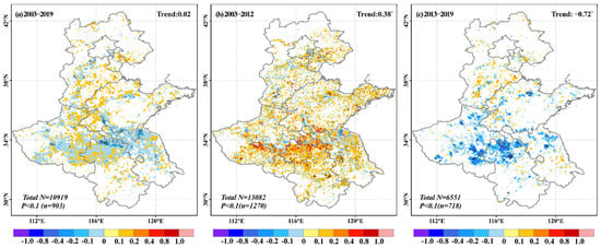
Figure 4.
Linear trends of CO2 emissions (unit: Gg yr−1) from crop residue burning in the NCP region estimated by the FRP-based method over the three periods of (a) 2003–2019, (b) 2003–2012, and (c) 2013–2019. The linear trend is calculated based on the least square method. Trends that are statistically significant above a 90% confidence level are marked with black borders, and the numbers of trends with a significant confidence level of about 90% are shown in the bottom left of each panel. Values inset in the upper right of each panel are linear regression trends for regional annual total crop residue burning emission over NCP, and those marked with * are statistically significant at a 95% confidence level.
3.3. Comparisons with Other Studies
The crop residue-burning emissions obtained in this work were compared with previously published studies for the same region and period to evaluate the estimations (Table 2). Generally, our results were in the same order of magnitude as the existing estimates. Take CO2 emission from crop residue burning as an example; the CO2 emissions were estimated within the range of 0.5 to 28.0 Tg reported for the NCP region of China [12,14,16,43,69,70]. The total annual mean CO2 emission was 2.35–11.45 Tg yr−1 based on the three different methods in our study. The estimates of emissions from crop residue burning using the BA-based method were substantially smaller than those of GFED4, which is based on the BA but with the correction on small fire burned area. It is also noted that our estimates of CO2 emission from crop residue burning over NCP in the year 2006 are somewhat lower than the values of 27.5 and 16.0 Tg reported by Huang et al. [12] and Liu et al. [14], which used statistical-based and FRP-based methods, respectively. This is mainly a result of the discrepancy in emission factors and other parameters used for estimations. Values of these parameters usually depend on the local agriculture practices and vary significantly in different studies. For example, the provincial crop-specific proportion of crop residues burned in the field ranges from 0.06 to 0.8 in different studies [70,71,72,73]. The emission factor for crop residue burning ranges from 1163.0 to 1723.0 (g kg−1) for CO2 estimation in different studies [10,12,25,29,69]. Regarding the FRP-based method, the combustion conversion ratio from energy to mass used in this work [31,37] is different from previous works. Generally, the comparison suggests that the estimates of crop residue-burning emissions in this work are within a reasonable range but highlights the need for the assessment of the spatial uncertainty in crop residue-burning emissions.
Table 2.
Comparison of CO2 emissions (Tg yr−1) from crop residue burning calculated in this work with the estimates made in previous studies.
3.4. Uncertainty Analysis
For each method, the uncertainty range in crop residue burning emission over NCP is quantified by using the Monte Carlo simulation. For statistical-based estimations, the uncertainties were associated with the total mass of in-field burning crop residues (Equation (1)) and EFs. Given the large statistical uncertainties assumed to be associated with such datasets, expert judgment was used to estimate the uncertainty in the amount of crop residue burning. Here, the uncertainty in the amount of crop residue burning was estimated to be 30%, which is the maximum value used in previous studies [75,76]. As for the BA-based method, the estimation uncertainties were related to the BA, available fuel loads, combustion efficiency factor, and EFs (Equation (4)). Following the reported values of previous works [44,77,78], the uncertainties of the BA data, available fuel loads, and combustion efficiency factors were estimated to be 30%, 20%, and 20%, respectively. For the FRP-based method, the uncertainties in emissions estimations were mainly caused by the FRP data, the conversion ratio and EFs (Equation (5)). In this work, we referred to the literature values and assumed the uncertainties in FRP and the conversion ratio to be 30% and 10%, respectively [16,34,79]. The reliability of EFs played an important role in driving uncertainty in all three methods. The uncertainties in the EFs of each pollutant are following to Huang et al. [12] and Ni et al. [25] and ranged from 6% to 50% (Table S3). As the uncertainties lower than ±60% were assumed to be normally distributed in most cases [80,81], all the parameters in each method were assumed to have a normal distribution, which was applied in previous works in China [16,77].
Considering all these parameters, 100,000 Monte Carlo simulations were conducted for pollutant emissions with a 95% confidence interval. The means and the uncertainty ranges of averaged annual crop residue burning emissions for each method are shown in Table S4. In general, the uncertainties of crop residue burning CO2 emissions from the statistical-based, BA-based, and FRP-based methods were (−17%, 26%), (−52%, 68%) and (−25%, 33%), respectively. For other gases and pollutants, the uncertainty ranges of estimations from the three methods were larger, which could be up to 103%, 138%, and 108% for statistical-based, BA-based, and FRP-based methods, respectively. The results showed that the uncertainties in the estimations based on the BA-method are the largest, followed by the FRP-based estimations and the statistical-based estimations. It should be noted that the uncertainty estimation for each method was strongly related to the assumed probability distribution and uncertainties in input parameters.
In addition to the uncertainty in each method, we also compared the emissions derived from different estimation methods. The emission gaps among the three different estimation approaches are significant, and Figure 5 presents the extent of variability in the three estimates for the period 2003–2019 at the grid level. Spatially, there are obvious variabilities among different estimates in the areas with low emission intensity, for which the maximum changes (CV) by up to 140% at the gridded level, while in the areas with high emission intensity, the uncertainties of crop residue burning emission inventories are relatively small, with the CV values ranging from 30% to 100%.
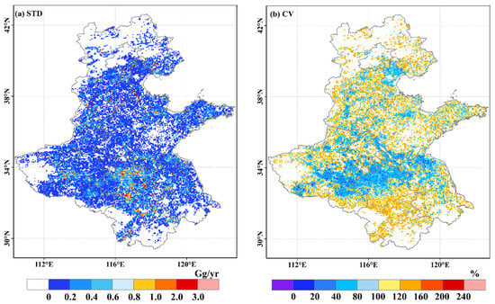
Figure 5.
(a) The gridded standard deviation (STD) and (b) coefficient of variation (CV) calculated based on the annual CO2 emission of crop residue burning from statistical-based, BA-based, and FRP-based methods over 2003–2019.
The range of crop residue-burning emissions of CO2, CO, CH4, NMHC, SO2, NH3, NOx, BC, OC, PM2.5, and PM10 over NCP according to the three methods are shown in Figure 6. For each species, the width of the box in Figure 6 may indicate the degree of variation in the estimations. The averaged total amount of CO2 emission calculated by the statistical-based method is more than three times higher than those calculated via FRP-based and BA-based methods. In general, the mean values of the three emissions of CO2, CO, CH4, NMHC, SO2, NH3, NOx, BC, OC, PM2.5, and PM10 over the period 2003–2018 are 5.532, 0.248, 0.015, 0.033, 0.002, 0.003, 0.014, 0.003, 0.018, 0.030, and 0.027 Tg yr−1, respectively, while the standard deviations of crop residue burning emissions in NCP are 4.94, 0.22, 0.013, 0.029, 0.002, 0.003, 0.013, 0.003, 0.016, 0.027, and 0.024 Tg yr−1, respectively.
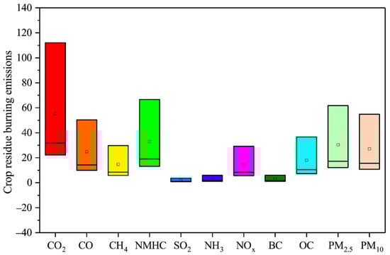
Figure 6.
Box-plots for annual emissions of CO2, CO, CH4, NMHC, SO2, NH3, NOx, BC, OC, PM2.5, and PM10 from crop residue burning obtained from the three methods (the units for all the species are Gg yr−1, but for clarity, the CO2 and CO emissions are scaled by a factor of 0.01 and 0.1, respectively). For each species, the bottom and top of the box are the maximum and minimum of the estimations, and the band inside the box is the median within the three methods. The width of the box indicates the degree of variation in the estimation.
4. Implication for the Impact of Crop Residue Burning Emission
The impact of the uncertainties in biomass burning emissions on CO2 simulation was quantified by performing several numerical simulations using the GEOS-Chem model. The distributions of simulated monthly mean CO2 concentrations of the standard simulation in June and October are presented in Figure 7a,b. Generally, CO2 concentrations in winter were higher than in other seasons due to large fossil fuel emissions and weak atmosphere-terrestrial exchange in cold seasons in NCP, which is consistent with previous studies [82]. For June, the highest CO2 concentrations were found in southeastern NCP, while the largest values in October were found in central NCP. The spatial distribution patterns are driven by the emissions, especially fossil fuel emission, and mediated by atmospheric transport. We tagged the CO2 emission from biomass burning in the standard simulation, and the results indicate that the biomass burning emission contributed 1.3 to 2.3 ppmv to the surface CO2 concentration in June and October in NCP (Figure 7c,d). This seems a rather small quantity for atmospheric CO2, but the magnitude of the contribution of biomass burning emissions to CO2 concentration in NCP is a few times larger than the changes of 0.25 ppmv in the Northern Hemisphere induced by the 7.9% reduction during the COVID-19 pandemic in the year 2020 [83], and the magnitude is equivalent to the interannual climate variability, for example, El Niño-Southern Oscillation (ENSO) induces biogenic CO2 changes of 1–3 ppmv [84,85].
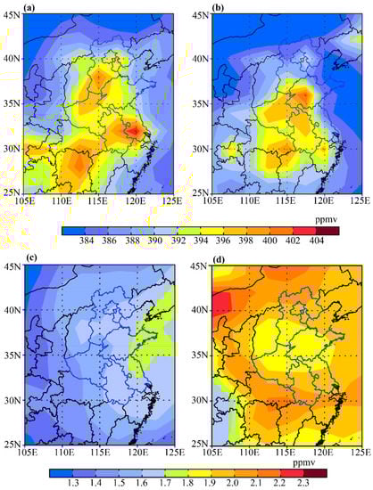
Figure 7.
Simulated surface CO2 concentration in (a) June and (b) October for the year 2018 over NCP from the standard simulation. (c,d) are the CO2 concentrations derived from biomass burning emission in June and October, respectively.
Next, we discuss the role of biomass burning emissions in shaping the CO2 concentration by comparing the results of the standard simulation (with biomass burning emissions) with those of the comparison simulation (without biomass burning emissions). The identified differences in CO2 concentration between the standard and comparison simulations could perhaps reflect the impact of biomass-burning emissions with a change of 100%. As expected, through an examination of the results of the standard simulation (Figure 7a,b), those of the comparison simulation present a similar spatial pattern with a bit lower value (not shown). Our results showed that the 100% reduction in biomass burning emissions might lead to a decrease in surface CO2 concentration by as much as 0.8–1.2 ppmv in NCP for the harvest time (Figure 8). This magnitude of change indicates that the effects of the uncertainties on existing biomass burning emission inventories may cause a substantial change in estimating the contribution of crop residue burning to atmospheric CO2 since large uncertainties were found for different sources of biomass burning emission inventories.
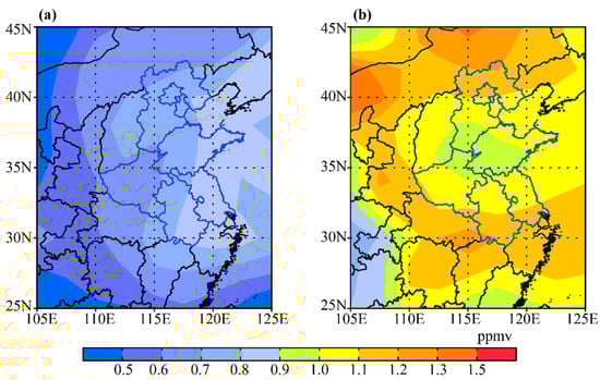
Figure 8.
(a,b) are the changes in surface CO2 concentration caused by the changes in biomass burning emissions for June and October, respectively (standard simulation minus comparison simulation).
5. Conclusions and Discussions
In this study, emissions from crop residue burning in the North China Plain (NCP) were investigated using three different methods, namely, statistical-based, BA-based, and FRP-based methods. The agreements and discrepancies in the spatiotemporal distribution of the three inventories for the period of 2003–2019 were compared, and the uncertainties in crop residue burning emission were examined. Overall, the estimates are consistent in both spatial distribution and temporal variation, despite obvious discrepancies in the total amount of the emissions. Spatially, crop residue burning is concentrated in the central and southern regions of the NCP. The results show that crop residue burning is high in June and October, which are the harvest times for winter wheat and summer corn in NCP.
The annual emissions of CO2, CO, CH4, NMHC, SO2, NH3, NOx, BC, OC, PM2.5, and PM10 averaged for three estimates over the period 2003–2018 were 5.532 ± 4.94, 0.248 ± 0.22, 0.015 ± 0.013, 0.033 ± 0.029, 0.002 ± 0.002, 0.003 ± 0.003, 0.014 ± 0.013, 0.003 ± 0.003, 0.018 ± 0.016, 0.030 ± 0.027, and 0.027 ± 0.024 Tg yr−1 (mean value ± standard deviation), respectively. The range of uncertainty in each estimate of crop residue burning over the NCP was quantified by Monte Carlo simulation, and the variations ranged from 20% to 70% for CO2 emissions at the regional level. The uncertainties of crop residue burning emissions are larger in low emission regions than those in high emission regions, which is mainly attributable to the uncertainties in small fire detection derived from satellite products. The coefficient of variation among the three estimates over NCP is within the range of 20% to 140% for hotspots at the gridded level.
Our results indicated that the statistical-based estimations are higher than those of BA-based and FRP-based estimations. Through contrastive analysis in this work, the advantages and shortcomings of each method were exhibited. The statistical-based method is necessary for estimating local emissions, while the accuracy of estimations for the large region using this method might be hampered by the sparse availability of statistical parameters. On the other hand, the satellite-based methods, including BA and FRP methods, are considered to be a reliable approach to constrain the estimations of emissions. In particular, the BA-based method is suitable for large fire emissions, such as forest or grassland fire, while the FRP-based method is suitable for small fire emissions, such as crop residue burning emissions. Hence, the estimations derived from the FRP-based method are considered to be more reasonable in spatial distribution and temporal variation, despite the emissions in this study are somewhat lower than the values reported in previous studies.
There are various sources of uncertainties in this study. The major uncertainties in the statistical-based estimations in this work arose from the accuracy and representativeness of the parameters (i.e., the residue-to-crop ratio, the dry fraction of crop residue, the proportion of crop residues burned in the field, etc.), as these parameters usually depend heavily on local agriculture practices and must be updated based on more field or laboratory measurements [16,72]. Regarding the BA-based method, the MCD64A1 tended to underestimate the burned crop area in coarse spatial resolution, as many fires in the cropland were less than 100 ha [67]. Previous studies have indicated that burned areas identified by satellites can be adjusted by a “small fire boost” methodology [86], or by using fractional vegetation cover and the degree of burning in pixels to reduce the uncertainty of BA [87,88]. However, these adjustments for the BA are not considered here. Another source of uncertainty in the BA-based method is related to the use of the available fuel load and combustion factor with a constant value for crops during the study period. Though the combustion factor in different periods among different vegetation varied significantly [18,35], the experimental data for the combustion factor of the crops are generally scarce and not consistent enough for inclusion in our estimation. For the FRP-based method, the associated conversion factor was obtained from the literature-extracted mean value, which may have caused uncertainties in estimations. A grided emission coefficient data developed based on satellite-driven FRP, and aerosol optical thickness is thought to be an important advance in fire emission estimations [36] and warrants further investigation in future studies. Additionally, the uncertainty in relation to the FRP-based methods is derived from the errors in satellite-derived active fire detections [16]. Recently, Zhang et al. [89,90] used a high-spatiotemporal resolution and small-fire-optimized VIIRS-IM FRP product with fire diurnal cycle information from the geostationary Himawari-8 satellite to estimate crop fire emissions and found that the FRP detected by the VIIRS-IM product is four times higher than that of the MODIS products in eastern China, which could lead to an increase in crop fires emissions by a factor of 0.5–4.7 compared to those reported by the GFAS and GFED 4.1 s. Furthermore, the accuracies in the land cover data are not explicitly taken into account in this study, which may yield part of the uncertainties in emission estimations.
The results of the model simulations show that the contribution of biomass-burning emissions had an important influence on the surface CO2 concentration (June and October), 1.0–2.0 ppmv, indicating a vital role of biomass burning emissions in atmospheric CO2 concentration during these seasons. The simulated monthly CO2 concentration varied by up to 0.8–1.2 ppmv due to the changes in biomass burning emissions. As reported by Zeng et al. [83], the observed reduction of 10–30 ppmv in Beijing and Chengdu was due to the reduced traffic and emissions as well as the weather variability during the COVID-19 lockdown. Although the magnitude of changes caused by biomass burning emissions is 10 times smaller than those changes, the impacts of biomass burning on CO2 concentration should not be ignored due to the large uncertainty in current estimations.
Finally, our study indicated that further investigations on improving parameterizations and promoting the accuracy of measurement and satellite instruments are needed to reconcile the differences between bottom-up and top-down methods. The findings in this work may give some limited insight into the impact of biomass burning emission on CO2 concentration due to the uncertainty in the emission inventories and atmospheric transport used in the model. More observations in this region would help us to make strong conclusions on understanding the influences of the uncertainty in biomass burning emissions.
Supplementary Materials
The following are available online at https://www.mdpi.com/article/10.3390/rs13193880/s1, Figure S1: Total crop productions (unit: million tons) over NCP from 2003 to 2018 derived from the National Bureau of Statistics of China, Figure S2: Linear trends of estimates of CO2 emission (Gg yr−1) from crop residue burning with significance at the 90% confidence level estimated by the FRP-based method over the three periods of 2003–2019, 2003–2012, and 2013–2019, respectively. (d,f) similar to (a–c), but for those trends with significance at the 95% confidence level. The numbers of trends significant at about the 90% or 95% confidence level are also shown in the upper right of each panel, Table S1: Crop-specific residue-to-production ratio, the dry fraction of crop residue and combustion factor for different crops, Table S2: Provincial crop-specific proportion of crop residues burned in the field (%) in the year 2012, Table S3: Emission factor (g kg−1 dry matter)and its uncertainty (%) for different pollutants, Table S4: Average annual crop residue burning emissions (Gg yr−1) over NCP during the study period. The values shown in parentheses are the uncertainty ranges of emissions in percentage change (%) that are relative to the mean.
Author Contributions
Conceptualization, Y.F.; Formal analysis, Y.F.; Funding acquisition, Y.F., H.L. and X.T.; Investigation, Y.F. and H.G.; Methodology, Y.F. and H.G.; Resources, Y.F. and H.G.; Software, H.G.; Supervision, H.L.; Visualization, Y.F. and H.G.; Writing—original draft, Y.F.; Writing—review and editing, H.G., H.L., and X.T. All authors have read and agreed to the published version of the manuscript.
Funding
This research was funded by the National Key Research and Development Program of China (2016YFA0600203 and 2019YFA0606802), and the National Natural Science Foundation of China (41977191).
Data Availability Statement
The data used to support the findings of this study are available from the corresponding author upon request.
Acknowledgments
We acknowledge the use of MODIS data products provided by Land Processes Distributed Active Archive Center (LP DAAC). We also thank NASA’s Science Computing Facility (SCF) at the University of Maryland for providing the FRP data. We acknowledge the efforts of the GEOS-Chem working groups for developing and managing the model. We would like to thank 4 anonymous reviewers for their helpful comments and suggestions on the improvement of the manuscript.
Conflicts of Interest
The authors declare no conflict of interest.
References
- Huang, X.; Song, Y.; Li, M.; Li, J.; Zhu, T. Harvest season, high polluted season in East China. Environ. Res. Lett. 2012, 7, 044033. [Google Scholar] [CrossRef]
- Ding, A.J.; Fu, C.B.; Yang, X.Q.; Sun, J.N.; Petäjä, T.; Kerminen, V.-M.; Wang, T.; Xie, Y.; Herrmann, E.; Zheng, L.F.; et al. Intense atmospheric pollution modifies weather: A case of mixed biomass burning with fossil fuel combustion pollution in eastern China. Atmos. Chem. Phys. 2013, 13, 10545–10554. [Google Scholar] [CrossRef] [Green Version]
- Cheng, Z.; Wang, S.; Fu, X.; Watson, J.G.; Jiang, J.; Fu, Q.; Chen, C.; Xu, B.; Yu, J.; Chow, J.C.; et al. Impact of biomass burning on haze pollution in the Yangtze River delta, China: A case study in summer 2011. Atmos. Chem. Phys. 2014, 14, 4573–4585. [Google Scholar] [CrossRef] [Green Version]
- Zhu, Y.; Yang, L.; Chen, J.; Wang, X.; Xue, L.; Sui, X.; Wen, L.; Xu, C.; Yao, L.; Zhang, J.; et al. Characteristics of ambient volatile organic compounds and the influence of biomass burning at a rural site in Northern China during summer 2013. Atmos. Environ. 2016, 124, 156–165. [Google Scholar] [CrossRef]
- Zhang, L.; Liu, Y.; Hao, L. Contributions of open crop straw burning emissions to PM2.5 concentrations in China. Environ. Res. Lett. 2016, 11, 014014. [Google Scholar] [CrossRef]
- Long, X.; Tie, X.; Cao, J.; Huang, R.; Feng, T.; Li, N.; Zhao, S.; Tian, J.; Li, G.; Zhang, Q. Impact of crop field burning and mountains on heavy haze in the North China Plain: A case study. Atmos. Chem. Phys. 2016, 16, 9675–9691. [Google Scholar] [CrossRef] [Green Version]
- Friedlingstein, P.; O’Sullivan, M.; Jones, M.W.; Friedlingstein, P.; O’sullivan, M.; Jones, M.W.; Andrew, R.M.; Hauck, J.; Olsen, A.; Peters, G.P.; et al. Global Carbon Budget 2020. Earth Syst. Sci. Data 2020, 12, 3269–3340. [Google Scholar] [CrossRef]
- Chen, J.; Li, C.; Ristovski, Z.; Milic, A.; Gu, Y.; Islam, M.S.; Wang, S.; Hao, J.; Zhang, H.; He, C.; et al. A review of biomass burning: Emissions and impacts on air quality, health and climate in China. Sci. Total Environ. 2017, 579, 1000–1034. [Google Scholar] [CrossRef] [Green Version]
- Mehmood, K.; Chang, S.; Yu, S.; Wang, L.; Li, P.; Li, Z.; Liu, W.; Rosenfeld, D.; Seinfeld, J.H. Spatial and temporal distributions of air pollutant emissions from open crop straw and biomass burnings in China from 2002 to 2016. Environ. Chem. Lett. 2018, 16, 301–309. [Google Scholar] [CrossRef]
- Zhang, T.; Wooster, M.; Green, D.; Main, B. New field-based agricultural biomass burning trace gas, PM2.5, and black carbon emission ratios and factors measured in situ at crop residue fires in Eastern China. Atmos. Environ. 2015, 121, 22–34. [Google Scholar] [CrossRef] [Green Version]
- Sun, J.; Peng, H.; Chen, J.; Wang, X.; Wei, M.; Li, W.; Yang, L.; Zhang, Q.; Wang, W.; Mellouki, A. An estimation of CO2 emission via agricultural crop residue open field burning in China from 1996 to 2013. J. Clean. Prod. 2016, 112, 2625–2631. [Google Scholar] [CrossRef]
- Huang, X.; Li, M.; Li, J.; Song, Y. A high-resolution emission inventory of crop burning in fields in China based on MODIS Thermal Anomalies/Fire products. Atmos. Environ. 2012, 50, 9–15. [Google Scholar] [CrossRef]
- McCarty, J.; Ellicott, E.A.; Romanenkov, V.; Rukhovitch, D.; Koroleva, P. Multi-year black carbon emissions from cropland burning in the Russian Federation. Atmos. Environ. 2012, 63, 223–238. [Google Scholar] [CrossRef]
- Liu, M.; Song, Y.; Yao, H.; Kang, Y.; Li, M.; Huang, X.; Hu, M. Estimating emissions from agricultural fires in the North China Plain based on MODIS fire radiative power. Atmos. Environ. 2015, 112, 326–334. [Google Scholar] [CrossRef]
- Qiu, X.; Duan, L.; Chai, F.; Wang, S.; Yu, Q.; Wang, S. Deriving High-Resolution Emission Inventory of Open Biomass Burning in China based on Satellite Observations. Environ. Sci. Technol. 2016, 50, 11779–11786. [Google Scholar] [CrossRef]
- Yin, L.; Du, P.; Zhang, M.; Liu, M.; Xu, T.; Song, Y. Estimation of emissions from biomass burning in China (2003–2017) based on MODIS fire radiative energy data. Biogeosciences 2019, 16, 1629–1640. [Google Scholar] [CrossRef] [Green Version]
- Li, J.; Li, Y.; Bo, Y.; Xie, S. High-resolution historical emission inventories of crop residue burning in fields in China for the period 1990–2013. Atmos. Environ. 2016, 138, 152–161. [Google Scholar] [CrossRef]
- Streets, D.G.; Yarber, K.F.; Woo, J.-H.; Carmichael, G.R. Biomass burning in Asia: Annual and seasonal estimates and atmospheric emissions. Glob. Biogeochem. Cycles 2003, 17, 1099. [Google Scholar] [CrossRef] [Green Version]
- Hoelzemann, J.J.; Schultz, M.; Brasseur, G.P.; Granier, C.; Simon, M. Global Wildland Fire Emission Model (GWEM): Evaluating the use of global area burnt satellite data. J. Geophys. Res. Space Phys. 2004, 109, 14. [Google Scholar] [CrossRef]
- Roy, B.A.; Pouliot, G.A.; Mobley, J.D.; Pace, T.G.; Pierce, T.E.; Soja, A.J.; Szykman, J.J.; Al-Saadi, J. Development of Fire Emissions Inventory Using Satellite Data. In Air Pollution Modeling and Its Application XIX; Springer: Berlin/Heidelberg, Germany, 2008; pp. 217–225. [Google Scholar]
- Shi, Y.; Yamaguchi, Y. A high-resolution and multi-year emissions inventory for biomass burning in Southeast Asia during 2001–2010. Atmos. Environ. 2014, 98, 8–16. [Google Scholar] [CrossRef]
- Shi, Y.; Matsunaga, T.; Saito, M.; Yamaguchi, Y.; Chen, X. Comparison of global inventories of CO2 emissions from biomass burning during 2002–2011 derived from multiple satellite products. Environ. Pollut. 2015, 206, 479–487. [Google Scholar] [CrossRef] [Green Version]
- Shi, Y.; Matsunaga, T. Temporal comparison of global inventories of CO2 emissions from biomass burning during 2002–2011 derived from remotely sensed data. Environ. Sci. Pollut. Res. 2017, 24, 16905–16916. [Google Scholar] [CrossRef]
- Wu, J.; Kong, S.; Wu, F.; Cheng, Y.; Zheng, S.; Qin, S.; Liu, X.; Yan, Q.; Zheng, H.; Zheng, M.; et al. The moving of high emission for biomass burning in China: View from multi-year emission estimation and human-driven forces. Environ. Int. 2020, 142, 105812. [Google Scholar] [CrossRef]
- Ni, H.; Han, Y.; Cao, J.; Chen, L.-W.; Tian, J.; Wang, X.; Chow, J.C.; Watson, J.; Wang, Q.; Wang, P.; et al. Emission characteristics of carbonaceous particles and trace gases from open burning of crop residues in China. Atmos. Environ. 2015, 123, 399–406. [Google Scholar] [CrossRef]
- Xu, Y.; Huang, Z.; Jia, G.; Fan, M.; Cheng, L.; Chen, L.; Shao, M.; Zheng, J. Regional discrepancies in spatiotemporal variations and driving forces of open crop residue burning emissions in China. Sci. Total Environ. 2019, 671, 536–547. [Google Scholar] [CrossRef] [PubMed]
- Vadrevu, K.P.; Giglio, L.; Justice, C. Satellite based analysis of fire–carbon monoxide relationships from forest and agricultural residue burning (2003–2011). Atmos. Environ. 2013, 64, 179–191. [Google Scholar] [CrossRef]
- Whitburn, S.; Van Damme, M.; Kaiser, J.; van der Werf, G.; Turquety, S.; Hurtmans, D.; Clarisse, L.; Clerbaux, C.; Coheur, P.-F. Ammonia emissions in tropical biomass burning regions: Comparison between satellite-derived emissions and bottom-up fire inventories. Atmos. Environ. 2015, 121, 42–54. [Google Scholar] [CrossRef]
- Seiler, W.; Crutzen, P.J. Estimates of gross and net fluxes of carbon between the biosphere and the atmosphere from biomass burning. Clim. Chang. 1980, 2, 207–247. [Google Scholar] [CrossRef]
- Song, Y.; Liu, B.; Miao, W.; Chang, D.; Zhang, Y. Spatiotemporal variation in nonagricultural open fire emissions in China from 2000 to 2007. Glob. Biogeochem. Cycles 2009, 23, 2008. [Google Scholar] [CrossRef]
- Wooster, M.J.; Roberts, G.; Perry, G.; Kaufman, Y.J. Retrieval of biomass combustion rates and totals from fire radiative power observations: FRP derivation and calibration relationships between biomass consumption and fire radiative energy release. J. Geophys. Res. Space Phys. 2005, 110, 24311. [Google Scholar] [CrossRef]
- Andela, N.; Kaiser, J.W.; van der Werf, G.R.; Wooster, M.J. New fire diurnal cycle characterizations to improve fire radiative energy assessments made from MODIS observations. Atmos. Chem. Phys. 2015, 15, 8831–8846. [Google Scholar] [CrossRef] [Green Version]
- Li, F.; Zhang, X.; Roy, D.P.; Kondragunta, S. Estimation of biomass-burning emissions by fusing the fire radiative power retrievals from polar-orbiting and geostationary satellites across the conterminous United States. Atmos. Environ. 2019, 211, 274–287. [Google Scholar] [CrossRef]
- Vermote, E.; Ellicott, E.; Dubovik, O.; Lapyonok, T.; Chin, M.; Giglio, L.; Roberts, G.J. An approach to estimate global biomass burning emissions of organic and black carbon from MODIS fire radiative power. J. Geophys. Res. Space Phys. 2009, 114, 18205. [Google Scholar] [CrossRef]
- Shi, Y.; Zang, S.; Matsunaga, T.; Yamaguchi, Y. A multi-year and high-resolution inventory of biomass burning emissions in tropical continents from 2001–2017 based on satellite observations. J. Clean. Prod. 2020, 270, 122511. [Google Scholar] [CrossRef]
- Ichoku, C.; Ellison, L. Global top-down smoke-aerosol emissions estimation using satellite fire radiative power measure-ments. Atmos. Chem. Phys. 2014, 14, 6643–6667. [Google Scholar] [CrossRef] [Green Version]
- Freeborn, P.H.; Wooster, M.; Hao, W.M.; Ryan, C.A.; Nordgren, B.L.; Baker, S.P.; Ichoku, C. Relationships between energy release, fuel mass loss, and trace gas and aerosol emissions during laboratory biomass fires. J. Geophys. Res. Space Phys. 2008, 113, 01301. [Google Scholar] [CrossRef]
- Ellicott, E.; Vermote, E.; Giglio, L.; Roberts, G. Estimating biomass consumed from fire using MODIS FRE. Geophys. Res. Lett. 2009, 36, L13401. [Google Scholar] [CrossRef] [Green Version]
- Wang, S.X.; Zhang, C.Y. Spatial and temporal distribution of air pollutant emissions from open burning of crop residues in China. Sci. Pap. Online 2008, 3, 329–333. (In Chinese) [Google Scholar]
- Liu, J.; Zheng, C.; Zheng, L.; Lei, Y. Ground Water Sustainability: Methodology and Application to the North China Plain. Ground Water 2008, 46, 897–909. [Google Scholar] [CrossRef]
- Li, X.; Wang, S.; Duan, L.; Hao, J.; Li, C.; Chen, Y.; Yang, L. Particulate and Trace Gas Emissions from Open Burning of Wheat Straw and Corn Stover in China. Environ. Sci. Technol. 2007, 41, 6052–6058. [Google Scholar] [CrossRef]
- He, M.; Zheng, J.; Yin, S.; Zhang, Y. Trends, temporal and spatial characteristics, and uncertainties in biomass burning emissions in the Pearl River Delta, China. Atmos. Environ. 2011, 45, 4051–4059. [Google Scholar] [CrossRef]
- Giglio, L. MODIS Collection 6 Active Fire Product User’s Guide, Revision B. 2018. Available online: https://cdn.earthdata.nasa.gov/conduit/upload/10575/MODIS_C6_Fire_User_Guide_B.pdf (accessed on 13 July 2021).
- Giglio, L.; Loboda, T.; Roy, D.P.; Quayle, B.; Justice, C.O. An active-fire based burned area mapping algorithm for the MODIS sensor. Remote Sens. Environ. 2009, 113, 408–420. [Google Scholar] [CrossRef]
- Giglio, L.; Boschetti, L.; Roy, D.P.; Humber, M.L.; Justice, C.O. The Collection 6 MODIS burned area mapping algorithm and product. Remote. Sens. Environ. 2018, 217, 72–85. [Google Scholar] [CrossRef]
- Zheng, J.; Zheng, Z.; Yu, Y.; Zhong, L. Temporal, spatial characteristics and uncertainty of biogenic VOC emissions in the Pearl River Delta region, China. Atmos. Environ. 2010, 44, 1960–1969. [Google Scholar] [CrossRef]
- Suntharalingam, P.; Jacob, D.J.; Palmer, P.; Logan, J.A.; Yantosca, R.M.; Xiao, Y.; Evans, M.J.; Streets, D.; Vay, S.L.; Sachse, G.W. Improved quantification of Chinese carbon fluxes using CO2/CO correlations in Asian outflow. J. Geophys. Res. Space Phys. 2004, 109, 109. [Google Scholar] [CrossRef]
- Nassar, R.; Jones, D.B.A.; Suntharalingam, P.; Chen, J.M.; Andres, R.J.; Wecht, K.J.; Yantosca, R.M.; Kulawik, S.S.; Bowman, K.W.; Worden, J.R.; et al. Modeling global atmospheric CO2 with improved emission inventories and CO2 production from the oxidation of other carbon species. Geosci. Model Dev. 2010, 3, 689–716. [Google Scholar] [CrossRef] [Green Version]
- Nassar, R.; Napier-Linton, L.; Gurney, K.R.; Andres, R.J.; Oda, T.; Vogel, F.R.; Deng, F. Improving the temporal and spatial distribution of CO2 emissions from global fossil fuel emission data sets. J. Geophys. Res. Atmos. 2013, 118, 917–933. [Google Scholar] [CrossRef]
- Shim, C.; Nassar, R.; Kim, J. Comparison of Model-simulated Atmospheric Carbon Dioxide with GOSAT Retrievals. Asian J. Atmos. Environ. 2011, 5, 263–277. [Google Scholar] [CrossRef] [Green Version]
- Chen, Z.H.; Zhu, J.; Zeng, N. Improved simulation of regional CO2 surface concentrations using GEOS-Chem and fluxes from VEGAS. Atmos. Chem. Phys. 2013, 13, 7607–7618. [Google Scholar] [CrossRef] [Green Version]
- Fu, Y.; Liao, H.; Tian, X.-J.; Gao, H.; Cai, Z.-N.; Han, R. Sensitivity of the simulated CO2 concentration to inter-annual variations of its sources and sinks over East Asia. Adv. Clim. Chang. Res. 2019, 10, 250–263. [Google Scholar] [CrossRef]
- Feng, L.; Palmer, P.I.; Yang, Y.; Yantosca, R.M.; Kawa, S.R.; Paris, J.-D.; Matsueda, H.; Machida, T. Evaluating a 3-D transport model of atmospheric CO2 using ground-based, aircraft, and space-borne data. Atmos. Chem. Phys. 2011, 11, 2789–2803. [Google Scholar] [CrossRef] [Green Version]
- Nassar, R.; Jones, D.B.A.; Kulawik, S.S.; Worden, J.R.; Bowman, K.W.; Andres, R.J.; Suntharalingam, P.; Chen, J.M.; Brenninkmeijer, C.A.M.; Schuck, T.J.; et al. Inverse modeling of CO2 sources and sinks using satellite observations of CO2 from TES and surface flask measurements. Atmos. Chem. Phys. 2011, 11, 6029–6047. [Google Scholar] [CrossRef] [Green Version]
- Liu, J.; Bowman, K.W.; Schimel, D.S.; Parazoo, N.C.; Jiang, Z.; Lee, M.; Bloom, A.A.; Wunch, D.; Frankenberg, C.; Sun, Y.; et al. Contrasting carbon cycle responses of the tropical continents to the 2015–2016 El Niño. Science 2017, 358, eaam5690. [Google Scholar] [CrossRef] [Green Version]
- Philip, S.; Johnson, M.S.; Potter, C.; Genovesse, V.; Baker, D.F.; Haynes, K.D.; Henze, D.K.; Liu, J.; Poulter, B. Prior biosphere model impact on global terrestrial CO2 fluxes estimated from OCO-2 retrievals. Atmos. Chem. Phys. 2019, 19, 13267–13287. [Google Scholar] [CrossRef] [Green Version]
- Gelaro, R.; McCarty, W.; Suárez, M.J.; Todling, R.; Molod, A.; Takacs, L.; Randles, C.A.; Darmenov, A.; Bosilovich, M.G.; Reichle, R.; et al. The Modern-Era Retrospective Analysis for Research and Applications, Version 2 (MERRA-2). J. Clim. 2017, 30, 5419–5454. [Google Scholar] [CrossRef]
- Oda, T.; Maksyutov, S. A very high-resolution (1 km × 1 km) global fossil fuel CO2 emission inventory derived using a point source database and satellite observations of nighttime lights. Atmos. Chem. Phys. 2011, 11, 543–556. [Google Scholar] [CrossRef] [Green Version]
- van der Werf, G.R.; Randerson, J.T.; Giglio, L.; Collatz, G.J.; Mu, M.; Kasibhatla, P.S.; Morton, D.C.; DeFries, R.S.; Jin, Y.; van Leeuwen, T.T. Global fire emissions and the contribution of deforestation, savanna, forest, agricultural, and peat fires (1997–2009). Atmos. Chem. Phys. 2010, 10, 11707–11735. [Google Scholar] [CrossRef] [Green Version]
- Yevich, R.; Logan, J.A. An assessment of biofuel use and burning of agricultural waste in the developing world. Global Biogeochem. Cycles 2003, 17, 1095. [Google Scholar] [CrossRef]
- Messerschmidt, J.; Parazoo, N.; Wunch, D.; Deutscher, N.M.; Roehl, C.; Warneke, T.; Wennberg, P.O. Evaluation of seasonal atmosphere–biosphere exchange estimations with TCCON measurements. Atmos. Chem. Phys. 2013, 13, 5103–5115. [Google Scholar] [CrossRef] [Green Version]
- Takahashi, T.; Sutherland, S.C.; Wanninkhof, R.; Sweeney, C.; Feely, R.A.; Chipman, D.W.; Hales, B.; Friederich, G.; Chavez, F.; Sabine, C.; et al. Climatological mean and decadal change in surface ocean pCO2, and net sea–air CO2 flux over the global oceans. Deep Sea Res. Part II Top. Stud. Oceanogr. 2009, 56, 554–577. [Google Scholar] [CrossRef]
- Corbett, J.J.; Koehler, H.W. Considering alternative input parameters in an activity-based ship fuel consumption and emissions model: Reply to comment by Øyvind Endresen et al. on “Updated emissions from ocean shipping”. J. Geophys. Res. Space Phys. 2004, 109, 23303. [Google Scholar] [CrossRef]
- Simone, N.W.; Stettler, M.E.J.; Barrett, S.R.H. Rapid estimation of global civil aviation emissions with uncertainty quantifica-tion. Transp. Res. Part D 2013, 25, 33–41. [Google Scholar] [CrossRef]
- Olsen, S.C.; Brasseur, G.P.; Wuebbles, D.J.; Barrett, S.R.; Dang, H.; Eastham, S.D.; Jacobson, M.Z.; Khodayari, A.; Selkirk, H.; Sokolov, A.; et al. Comparison of model estimates of the effects of aviation emissions on atmospheric ozone and methane. Geophys. Res. Lett. 2013, 40, 6004–6009. [Google Scholar] [CrossRef] [Green Version]
- Randerson, J.T.; Chen, Y.; van der Werf, G.; Rogers, B.M.; Morton, D.C. Global burned area and biomass burning emissions from small fires. J. Geophys. Res. Space Phys. 2012, 117, 04012. [Google Scholar] [CrossRef]
- Zhu, C.; Kobayashi, H.; Kanaya, Y.; Saito, M. Size-dependent validation of MODIS MCD64A1 burned area over six vegetation types in boreal Eurasia: Large underestimation in croplands. Sci. Rep. 2017, 7, 4181. [Google Scholar] [CrossRef] [PubMed]
- Tao, S.; Ru, M.Y.; Du, W.; Zhu, X.; Zhong, Q.; Li, B.G.; Shen, G.F.; Pan, X.L.; Meng, W.J.; Chen, Y.L.; et al. Quantifying the rural residential energy transition in China from 1992 to 2012 through a representative national survey. Nat. Energy 2018, 3, 567–573. [Google Scholar] [CrossRef]
- Wiedinmyer, C.; Akagi, S.K.; Yokelson, R.J.; Emmons, L.K.; Al-Saadi, J.A.; Orlando, J.J.; Soja, A.J. The Fire INventory from NCAR (FINN): A high resolution global model to estimate the emissions from open burning. Geosci. Model Dev. 2011, 4, 625–641. [Google Scholar] [CrossRef] [Green Version]
- van der Werf, G.R.; Randerson, J.T.; Giglio, L.; van Leeuwen, T.T.; Chen, Y.; Rogers, B.M.; Mu, M.; van Marle, M.J.E.; Morton, D.C.; Collatz, G.J.; et al. Global fire emissions estimates during 1997–2016. Earth Syst. Sci. Data 2017, 9, 697–720. [Google Scholar] [CrossRef] [Green Version]
- Gao, X.; Ma, W.; Ma, C.; Zhang, F.; Wang, Y. Analysis on the current status of utilization of crop straw in China. J. Huazhong Agric. Univ. 2002, 21, 242–247. (In Chinese) [Google Scholar]
- Yan, X.; Ohara, T.; Akimoto, H. Bottom-up estimate of biomass burning in mainland China. Atmos. Environ. 2006, 40, 5262–5273. [Google Scholar] [CrossRef]
- Yang, S.; He, H.; Lu, S.; Chen, D.; Zhu, J. Quantification of crop residue burning in the field and its influence on ambient air quality in Suqian, China. Atmos. Environ. 2008, 42, 1961–1969. [Google Scholar] [CrossRef]
- Kaiser, J.W.; Heil, A.; Andreae, M.O.; Benedetti, A.; Chubarova, N.; Jones, L.; Morcrette, J.J.; Razinger, M.; Schultz, M.G.; Suttie, M.; et al. Biomass burning emissions estimated with a global fire assimilation system based on observed fire radiative power. Biogeosciences 2012, 9, 527–554. [Google Scholar] [CrossRef] [Green Version]
- Zhao, Y.; Nielsen, C.P.; Lei, Y.; McElroy, M.B.; Hao, J. Quantifying the uncertainties of a bottom-up emission inventory of anthropogenic at-mospheric pollutants in China. Atmos. Chem. Phys. 2011, 11, 2295–2308. [Google Scholar] [CrossRef] [Green Version]
- Zhang, Y.; Shao, M.; Lin, Y.; Luan, S.; Mao, N.; Chen, W.; Wang, M. Emission inventory of carbonaceous pollutants from biomass burning in the Pearl River Delta Region, China. Atmos. Environ. 2013, 76, 189–199. [Google Scholar] [CrossRef]
- Wu, J.; Kong, S.; Wu, F.; Cheng, Y.; Zheng, S.; Yan, Q.; Zheng, H.; Yang, G.; Zheng, M.; Liu, D.; et al. Estimating the open biomass burning emissions in central and eastern China from 2003 to 2015 based on satellite observation. Atmos. Chem. Phys. 2018, 18, 11623–11646. [Google Scholar] [CrossRef] [Green Version]
- Shi, Y.; Matsunaga, T.; Yamaguchi, Y. High-Resolution Mapping of Biomass Burning Emissions in Three Tropical Regions. Environ. Sci. Technol. 2015, 49, 10806–10814. [Google Scholar] [CrossRef] [PubMed]
- Freeborn, P.H.; Wooster, M.J.; Roy, D.P.; Cochrane, M.A. Quantification of MODIS fire radiative power (FRP) measurement uncertainty for use in satellite-based active fire characterization and biomass burning estimation. Geophys. Res. Lett. 2014, 41, 1988–1994. [Google Scholar] [CrossRef]
- Monni, S.; Syri, S.; Savolainen, I. Uncertainties in the Finnish greenhouse gas emission inventory. Environ. Sci. Policy 2004, 7, 87–98. [Google Scholar] [CrossRef]
- Ramírez, A.; de Keizer, C.; Van der Sluijs, J.P.; Olivier, J.; Brandes, L. Monte Carlo analysis of uncertainties in the Nether-lands greenhouse gas emission inventory for 1990–2004. Atmos. Environ. 2008, 42, 8263–8272. [Google Scholar] [CrossRef] [Green Version]
- Kou, X.; Zhang, M.; Peng, Z.; Wang, Y. Assessment of the biospheric contribution to surface atmospheric CO2 concentrations over East Asia with a regional chemical transport model. Adv. Atmos. Sci. 2015, 32, 287–300. [Google Scholar] [CrossRef]
- Zeng, N.; Han, P.; Liu, D.; Liu, Z.; Oda, T.; Martin, C.; Liu, Z.; Yao, B.; Sun, W.; Wang, P.; et al. Global to local impacts on atmospheric CO2 caused by COVID-19 lockdown. arXiv 2020, arXiv:2010.13025. Available online: https://arxiv.org/abs/2010.13025v1 (accessed on 23 September 2021).
- Zeng, N.; Mariotti, A.; Wetzel, P. Terrestrial mechanisms of interannual CO2 variability. Glob. Biogeochem. Cycles 2005, 19, 1016. [Google Scholar] [CrossRef]
- Graven, H.D.; Keeling, R.F.; Piper, S.C.; Patra, P.K.; Stephens, B.B.; Wofsy, S.C.; Welp, L.R.; Sweeney, C.; Tans, P.P.; Kelley, J.J.; et al. Enhanced Seasonal Exchange of CO2 by Northern Ecosystems Since 1960. Science 2013, 341, 1085–1089. [Google Scholar] [CrossRef] [Green Version]
- Zhang, T.; Wooster, M.J.; de Jong, M.C.; Xu, W. How Well Does the ‘Small Fire Boost’ Methodology Used within the GFED4.1s Fire Emissions Database Represent the Timing, Location and Magnitude of Agricultural Burning? Remote Sens. 2018, 10, 823. [Google Scholar] [CrossRef] [Green Version]
- Gao, H.; Zhang, J.; Zheng, W.; Liu, C. Comparative study on the emission estimation from the forest fire based on different resolution satellite data. Geogr. Res. 2017, 36, 850–860. [Google Scholar]
- Chen, J.; Zheng, W.; Gao, H.; Shao, J.; Liu, C. Estimation method of straw burned area based on multi-source satellite remote sensing. Trans. Chin. Soc. Agric. Eng. 2015, 31, 207–214, (In Chinese with English abstract). [Google Scholar]
- Zhang, T.; Wooster, M.; Xu, W. Approaches for synergistically exploiting VIIRS I- and M-Band data in regional active fire detection and FRP assessment: A demonstration with respect to agricultural residue burning in Eastern China. Remote Sens. Environ. 2017, 198, 407–424. [Google Scholar] [CrossRef] [Green Version]
- Zhang, T.; de Jong, M.C.; Wooster, M.J.; Xu, W.; Wang, L. Trends in eastern China agricultural fire emissions derived from a combination of geostationary (Himawari) and polar (VIIRS) orbiter fire radiative power products. Atmos. Chem. Phys. 2020, 20, 10687–10705. [Google Scholar] [CrossRef]
Publisher’s Note: MDPI stays neutral with regard to jurisdictional claims in published maps and institutional affiliations. |
© 2021 by the authors. Licensee MDPI, Basel, Switzerland. This article is an open access article distributed under the terms and conditions of the Creative Commons Attribution (CC BY) license (https://creativecommons.org/licenses/by/4.0/).