Change Detection Using a Texture Feature Space Outlier Index from Mono-Temporal Remote Sensing Images and Vector Data

Abstract

Multi-temporal remote sensing images are the primary sources for change detection. However, it is difficult to obtain comparable multi-temporal images at the same season and time of day with the same sensor. Considering texture homogeneity among objects belonging to the same category, this paper presents a new change detection approach using a texture feature space outlier index from mono-temporal remote sensing images and vector data. In the proposed approach, a texture feature contribution index (TFCI) is defined based on information gain to select the optimal texture features, and a feature space outlier index (FSOI) based on local reachability density is presented to automatically identify outlier samples and changed objects. Our approach includes three steps: (1) the sampling method is designed considering spatial distribution and topographic properties of image objects extracted by segmenting the recent image with existing vector map. (2) Samples with changed categories are refined by an iteration procedure of texture feature selection and outlier sample elimination; and (3) the changed image objects are identified and classified using the refined samples to calculate the FSOI values of the image objects. Three experiments in the two study areas were conducted to validate its performance. Overall accuracies of 95.94%, 96.36%, and 96.28% were achieved, respectively, while the omission and commission errors for every category were all very low. Four widely used methods with two-temporal images were selected for comparison, and the accuracy of the proposed method is higher than theirs. This indicates that our approach is effective and feasible.

1. Introduction

Change detection of the Earth’s surface features is the process of measuring the landscape changes of the same geographical area at different times [1,2,3]. It is extremely important for monitoring disasters and observing urban expansion as well as ecosystem and land-use/land-cover changes [4,5,6,7,8]. Due to the advantages of repetitive data acquisition, its synoptic view, low cost, and fast response capacities, remote sensing has long been recognized as an effective tool for a variety of change detection applications [9,10,11].

At present, multi-temporal remote sensing images are the primary sources used for a variety of change detection applications [1,12,13], and researchers have developed a series of change detection methods with multi-temporal images, such as direct comparison methods (e.g., change vector analysis and image differencing) [14,15,16,17], post-classification comparison (PCC) [18,19], object-based methods (OBMs) [20], hybrid change detection [21,22], machine learning (e.g., support vector machine (SVM), random forest (RF), and artificial neural network) [23,24,25], and deep-learning-based methods (DLMs) [26,27]. Various researchers have exhaustively highlighted the shortfalls and application aspects of these change detection techniques [12,13,28]. For example, the difficulty with the direct comparison methods is the identification of changed trajectories and the strict requirement of image data acquired from the same phenological period with the same sensor [29,30]. PCC requires an accurate and complete training data set, and final accuracy is dependent on the classification accuracy of individual images [31,32]. Machine learning has some difficulty in choosing training samples, and the computational time for classification and achieving optimization during the learning phase increases polynomially with the increase of data dimensionality [33,34]. The main issues with DLMs are that it is sensitive to the training data quality and the number of training samples per class [35,36]. All of these above methods require at least two-temporal comparable images [37,38]. However, it is usually very difficult to acquire comparable multi-temporal images that can meet all of the above criteria, because there are many factors that impact the spectral features of surface objects, such as sensors, phenological characteristics, and environmental factors. Therefore, change detection that uses an additional easily obtainable data source (e.g., vector data and digital elevation model (DEM)) has become a popular research topic [39,40,41].

On one hand, vector data includes a priori information such as location, shape, size, and categories, which allow the user to exploit the geometric information (e.g., location and shape) of objects, reducing the search space and minimizing false alarms [28,42]. On the other hand, with the construction of all kinds of geodatabases (e.g., GlobeLand30), vector data for many application requirements of change detection can be obtained from the existing geodatabases [4,43]. In recent years, vector data have been widely used as a major additional source of data to improve the change detection accuracy of remote sensing images. However, these approaches using vector data are limited in most cases to the comparison of image-vector objects [28,39]. For example, Li et al. [41] described a buffer-detection algorithm and an integrated approach with vector data for change detection of linear and area features, respectively. Sofina and Ehlers et al. [38] proposed a new “detected part of contour” feature with vector data for building change detection. De Alwis Pitts and So et al. [44] utilized readily available pre-disaster vector data and two high-resolution images to enhance change detection for disaster response. Lopez et al. [45] utilized high-resolution SAR images and a priori knowledge about the imaged scene from vector maps to perform change detection of ship activity. Guo and Du et al. [39] integrated high-resolution images and vector data to acquire knowledge of building extraction and change detection, such as optimal segmentation scales, samples, and the feature subsets. The effectiveness of these change detection methods is close to or higher than the image-based methods. However, due to the complexity of surface landscapes in the high-resolution remote sensing images, challenges still remain in applying vector data and images for change detection. For example, it is still difficult to automatically identify the changed objects and determine their types. Accordingly, it is necessary to further investigate the integration of vector data and remote sensing images for change detection.

Considering texture homogeneity among objects belonging to the same categories, this paper presents an object-texture-outlier (OTO)-based change detection approach. In the proposed method, the vector data is used as a substitute for historic remote sensing images. The image objects are extracted by segmenting image with existing vector data. Changed objects are identified by comparing texture heterogeneity among image objects which have the same a priori categories. Compared with unchanged objects, the changed image objects are described as outlier objects according to texture heterogeneity. Texture features are used to measure the space outlier of image objects. However, how to automatically select the optimal texture features for every category, identify changed objects, and determine their types are still critical issues that need to be addressed. First, a texture feature contribution index (TFCI) is defined based on information gain to select the optimal texture features for each category. Second, a feature space outlier index (FSOI) based on local reachability density is presented to automatically identify outlier samples and changed objects. Samples with changed categories are refined by an iteration procedure of texture feature selection and outlier sample elimination. The types of the changed objects are determined with the refined samples.

The remainder of this paper is organized such that Section 2 outlines the proposed change detection method, including the sampling design, sample refinement by the iteration of texture feature selection and outlier sample elimination, and the changed object detection. The results and discussion are presented in Section 3 and Section 4, respectively. Finally, the main conclusions are drawn in Section 5.

2. Methods

The framework of the proposed change detection approach from mono-temporal remote sensing images and vector data is shown in Figure 1. Our approach involves three main steps. (1) The sampling design is based on a priori information. Image objects are first extracted by segmenting the recent images with the existing vector map, which can significantly reduce the difficulty and improve accuracy of image segmentation. The extracted image objects are bundled with a priori information (e.g., shape and category) from vector data and spectral information from the images. Then, the sampling method is designed considering the spatial distribution and topographic properties of the objects (DEM data are used to represent the topographic properties), and the initial samples are obtained, although there may be some samples with changed categories. (2) Samples with changed categories are refined by an iteration procedure in which texture features are selected and outlier samples are eliminated. In the iteration procedure, a TFCI is defined based on information gain to select the optimal texture features, and an FSOI based on local reachability density is presented to automatically identify outlier samples. After the iteration, the optimal texture features for each category can be determined, and the samples with unchanged categories can be obtained. (3) The detection and classification of the changed objects are conducted. The changed objects are identified with the refined samples by calculating the FSOI values of image objects. The changed image objects are resegmented based on the existing multi-resolution segmentation algorithm [46,47], and the resegmented changed image objects are classified with the refined samples by calculating the FSOI values of the image objects. In this paper, the sampling design, sample refinement (including TFCI and FSOI), and changed object detection are all discussed in detail.

2.1. Sampling Design with a Priori Information from Vector Data and DEM

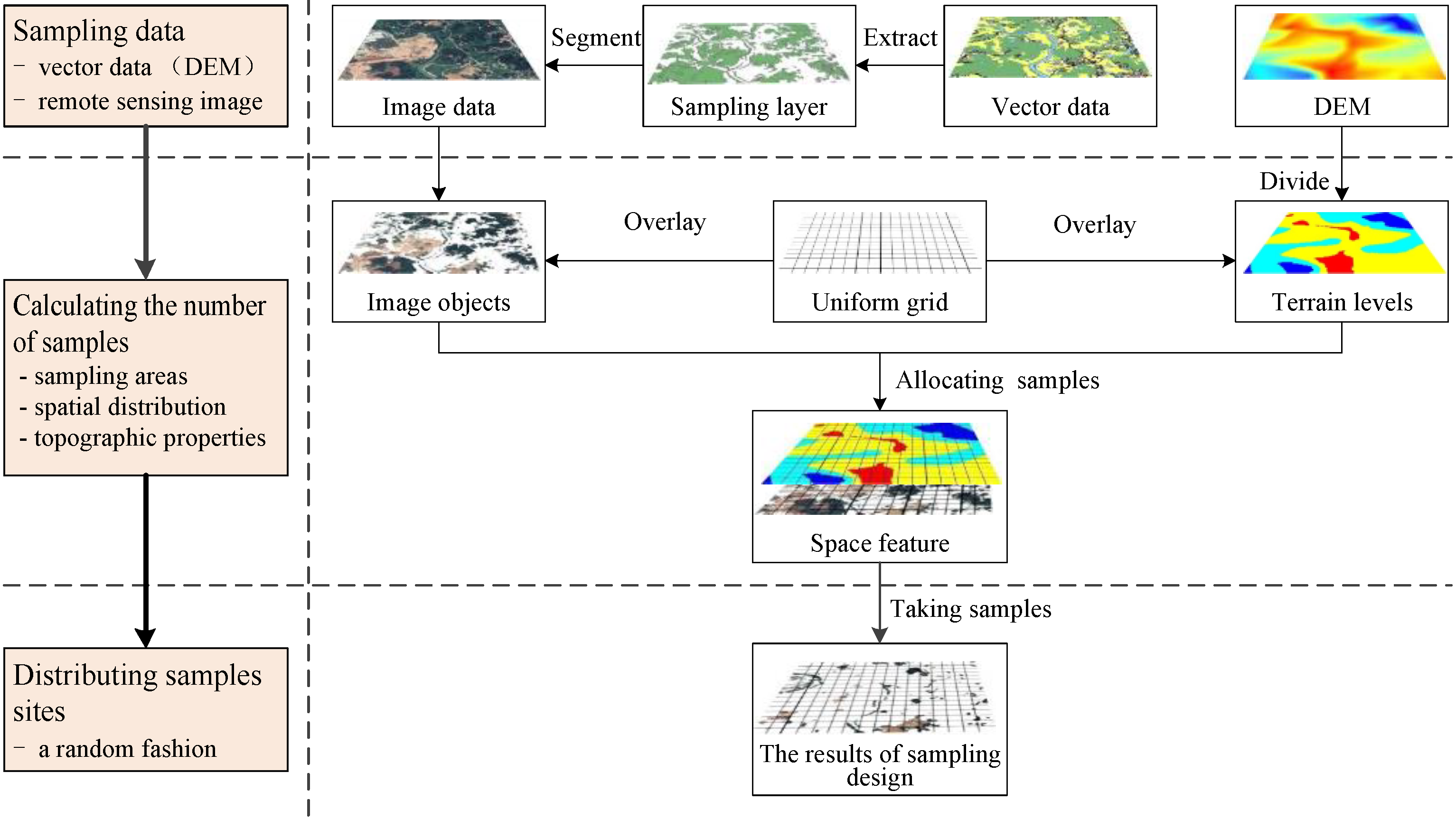
It is well known that the quality of samples determines the success of the change detection process, while the quality of samples is affected by the size and location distribution of sample objects [48]. Besides, the quality of samples is also affected by their representativeness. When the vector map is available, all objects can be theoretically used as samples. However, this will decrease the representativeness of samples. Considering the above reasons, we choose the representative objects as the samples. Therefore, the sampling design is one of the key steps in implementing automatic sampling for change detection. Since samples are taken from image objects that have the same a priori categories, the image objects that have changed in a posteriori category are inevitably sampled. Compared to the number of unchanged objects, the number of changed objects is usually expected to be small. The aim of sampling design is to obtain as few as possible changed samples and enough statistical power to detect texture homogeneity among objects belonging to the same categories. The appropriate sampling area, density of sampling, and allocation of sampling sites are three important characteristics to be considered when designing a sampling program. The sampling area selection should be based on requirements for outlier data and specific study areas. The probability of image objects with homogeneous texture features being sampled will increase with the enlargement of the sampling range, so the sampling design requires sampling at a global range in the study area. The density of sampling (i.e., the number of samples per unit area) is usually dictated by the practical constraints of the landscape and topographic properties. Sampling sites must be distributed in a purely random fashion. Consequently, sampling design is achieved according to sampling areas, spatial distribution, and the topographic properties of the objects.

A uniform grid that covers the sampling area is used to allocate samples. First, the sampling area is divided into a uniform grid. The size of the grid can be properly determined according to the size of the sampling area, the total number of image objects, and the number of samples taken. Second, the sampling area is divided into t levels according to topographic properties based on DEM data, and then the number of samples is calculated in each cell. The number of samples in row r and column c of the grid, ${\mathrm{SN}}_{r\times c}$, is calculated as follows:

$${\mathrm{SN}}_{r\times c}={\displaystyle \sum _{j=1}^{\mathrm{t}}\frac{{\mathrm{Ion}}_{r\times c}^j}{\mathrm{Ion}}}\mathrm{STN}$$

(1)

where Ion is the number of objects and STN is the number of samples taken in the sampling area. ${\mathrm{Ion}}_{r\times c}^j$ is the number of objects in row r and column c of the terrain level j. The principle of sampling design is shown in Figure 2. Finally, samples for each cell are randomly taken from objects included in each cell, and the initial samples containing outlier samples (i.e., changed sample objects) are obtained.

2.2. Refining Samples by Iteration of Texture Feature Selection and Outlier Sample Elimination

To improve the accuracy of the change detection results, a TFCI is defined by information gain to select the optimal texture features for each category, and an FSOI based on local reachability density is presented to automatically identify outlier samples and changed objects. However, the optimal texture features need to be identified from samples with unchanged categories, and samples with unchanged categories need to be extracted according to the optimal texture features. Therefore, automatically identifying the optimal texture features is in contradiction with automatically detecting outlier samples. Consequently, in order to implement automatic sampling for change detection, samples with changed categories must be refined by an iteration procedure of texture feature selection and outlier sample elimination.

2.2.1. TFCI Computation Based on Information Gain

Texture is an innate property of all types of surface objects and contains important information about the structural arrangement of surfaces and their relationship to the surrounding environment [49,50]. Texture information is widely used to help in segmentation or classification. Among multitudinous texture analysis methods, a gray-level co-occurrence matrix (GLCM) has been proven to be an effective tool for capturing numerical features of remote sensing images using spatial relations of similar gray tones [51,52]. The 14 texture features have been defined based on the GLCM [50], as shown in

Table 1. The 14 texture features and their serial numbers.

Serial Number	Texture Features
f1	Angular Second Moment (ASM)
f2	Contrast (CON)
f3	Inverse Difference Moment (IDM)
f4	Entropy (ENT)
f5	Correlation (COR)
f6	Mean (MEAN)
f7	Variance (VAR)
f8	Sum Variance (SVAR)
f9	Sum Average (SAVE)
f10	Sum Entropy (SENT)
f11	Difference Entropy (DENT)
f12	Difference Variance (DVAR)
f13	Information Measures of Correlation (IMC)
f14	Maximal Correlation Coefficient (MCC)

.

Directly applying all of the texture features from the GLCM to describe the texture information results in some redundancy because some of the features may not have a clear contribution to distinguishing different categories of image objects. The redundancy is related to the uncertainty of texture feature values. Therefore, identifying the optimal texture features can be accomplished by analyzing the uncertainty of different texture features. It is well known that information entropy is regarded as an effective tool to measure the uncertainty [27,53], and thus, information entropy is used to measure the contribution of a texture feature to distinguish different categories of image objects.

The information gain is a measure of the decrease in the amount of information entropy that one feature has about all other features [54]. It can be used as an index to measure the importance of texture features. Assume that $\mathrm{Gain}(c_i,f_j)$ indicates the information gain of texture feature $f_j$ belonging to category $c_i$, and the expression of $\mathrm{Gain}(c_i,f_j)$ can be written as:

$$\begin{array}{l}\mathrm{Gain}(c_i,f_j)=\mathrm{H}(c_i)-\mathrm{H}(c_i/f_j)\\ \mathrm{H}(c_i)=-\{p_{c_i}\log (p_{c_i})+(1-p_{c_i})\log (1-p_{c_i})\}\\ \mathrm{H}(c_i/f_j)=-p_{f_j}\{p_{c_i{f}_j}\log (p_{c_i{f}_j})+(1-p_{c_i{f}_j})\log (1-p_{c_i{f}_j})\}\\ p_{c_i}=N_{c_i}/N;p_{f_j}=N_{c_i{f}_j}/N;p_{c_i{f}_j}=N_{c_i}/N_{c_i{f}_j}\end{array}$$

(2)

where $\mathrm{H}(c_i)$ is information entropy and $\mathrm{H}(c_i/f_j)$ is conditional information entropy of category $c_i$. N is the total number of objects and $N_{c_i}$ is the number of objects belonging to category $c_i$. $N_{c_i{f}_j}$ is the number of objects whose values of texture feature $f_j$ belong to the texture feature space of the category $c_i$. However, applying information gain may result in a biased estimation that the optimal texture features tend to have a larger range of the feature vector [55]. Hence, the information gain ratio is employed to eliminate this effect. Assuming that $\mathrm{GainRat}(c_i,f_j)$ represents the information gain ratio of texture feature f_j belonging to the category $c_i$, and $\mathrm{GainRat}(c_i,f_j)$ can be written as:

$$\begin{array}{l}\mathrm{GainRat}(c_i,f_j)=\mathrm{Gain}(c_i,f_j)/\mathrm{H}(f_j)\\ \mathrm{H}(f_j)=-\{p_{f_j}\log (p_{f_j})+(1-p_{f_j})\log (1-p_{f_j})\}\end{array}$$

(3)

where $\mathrm{H}(f_j)$ is the information entropy of texture feature $f_j$. Therefore, a texture feature contribution index (TFCI) based on information gain ratio can be defined as:

$${\mathrm{TFCI}}_{f_j{c}_i}=\frac{\mathrm{GainRat}(c_i,f_j)\times 100\%}{{\max }_c\{\mathrm{GainRat}(c_i,f_j)/{\max }_f(\mathrm{GainRat}(c_i,f_j))\}}$$

(4)

where ${\mathrm{TFCI}}_{f_j{c}_i}$ indicates the TFCI of the texture feature $f_j$ belonging to the category $c_i$. The TFCI value is between 0 and 100%, and the higher its value, the greater the contribution of texture feature $f_j$ on category $c_i$. Hence, it is easy to determine which texture features can be selected as the optimal features to identify changed objects. In order to quantify the contribution levels of texture features, analytic hierarchy process (AHP) is used to determine the priorities of texture feature selection. In AHP for texture features, the equal interval method is applied to divide the TFCI interval into five sub-intervals, and each sub-interval width is equal to all other sub-interval widths [56,57].

Table 2. Five hierarchy numbers and their contribution levels of texture feature contribution index (TFCI).

Hierarchy Number	TFCI Value	Contribution Level
I	[0, 20]	Very low contribution
II	(20, 40]	Low contribution
III	(40, 60]	Moderate contribution
IV	(60, 80]	High contribution
V	(80, 100]	Very high contribution

shows the five sub-intervals and their contribution levels.

The optimal texture features can be selected according to the TFCI value. Generally, the texture features with very low and low contribution levels must be eliminated, texture features with moderate contribution levels can be selected appropriately, and texture features with high and very high contribution levels must be selected.

The texture feature space vector (TFSV) for types of surface objects can be established according to the results of the optimal texture feature selection. Assume that $\mathrm{TFSV}(c_j)$ indicates the TFSV of the category $c_j$. The expression of $\mathrm{TFSV}(c_j)$ can be written as:

$$\mathrm{TFSV}(c_j)={[w_1^j{f}_1,w_2^j{f}_2,\cdots ,w_{14}^j{f}_{14}]}^{\mathrm{T}}$$

(5)

where $w_{{}_i}^j(i=1,2,\cdots ,14)$ is TFCI value of texture feature $f_i$ in the category $c_j$. In Equation (5), if TFCI values of texture feature $f_i$ are below 60%, texture feature $f_i$ should not be chosen, and the $w_{{}_i}^j$ value is set as zero.

2.2.2. FSOI Computation Based on Local Reachability Density

In remote sensing images, there are many factors that impact the spectral features of surface objects, including sensors, phenological characteristics, and environmental factors, as well as changes in the types of surface objects caused by man or sudden natural disasters. However, change detection aims to identify changed objects caused by man or such natural disasters. The texture features of changed objects have clear outlier characteristics, both in samples and change detection. Some scholars describe the concept of an outlier from different aspects [58,59,60]. Intuitively, an outlier is an observation that deviates so much from other observations that it arouses suspicion that it is generated by a different mechanism [61,62]. In this paper, the outlier data can be defined as data sets of low-density areas in the texture feature space (e.g., changed image objects). Consequently, the outlier detection idea is employed to detect outlier samples and changed objects.

Some researchers have proposed the method of calculating density outlier according to the spatial distribution characteristics of outlier data [63,64]. However, for outlier image objects that need to be detected, there may be a large number of outlier objects with the same or similar texture features. In order to detect outlier data more accurately, a feature space outlier index (FSOI) is defined to detect outlier samples and changed objects based on the local reachable density and global characteristics of image objects. In addition, this paper designs an iteration procedure (described in Figure 1) to refine unchanged samples. The FSOI can be calculated through three steps as follows.

The first step is to calculate the reachability distance of an object in texture feature space. Let ${\mathrm{Rdis}}_k\left(o{b}_j,o{b}_i\right)$ denote the reachability k_distance of object $o{b}_i$ with respect to object $o{b}_j$, and it is defined as:

$${\mathrm{Rdis}}_k(o{b}_j,o{b}_i)=\max (k\_dis(o{b}_i),d(o{b}_j,o{b}_i))$$

(6)

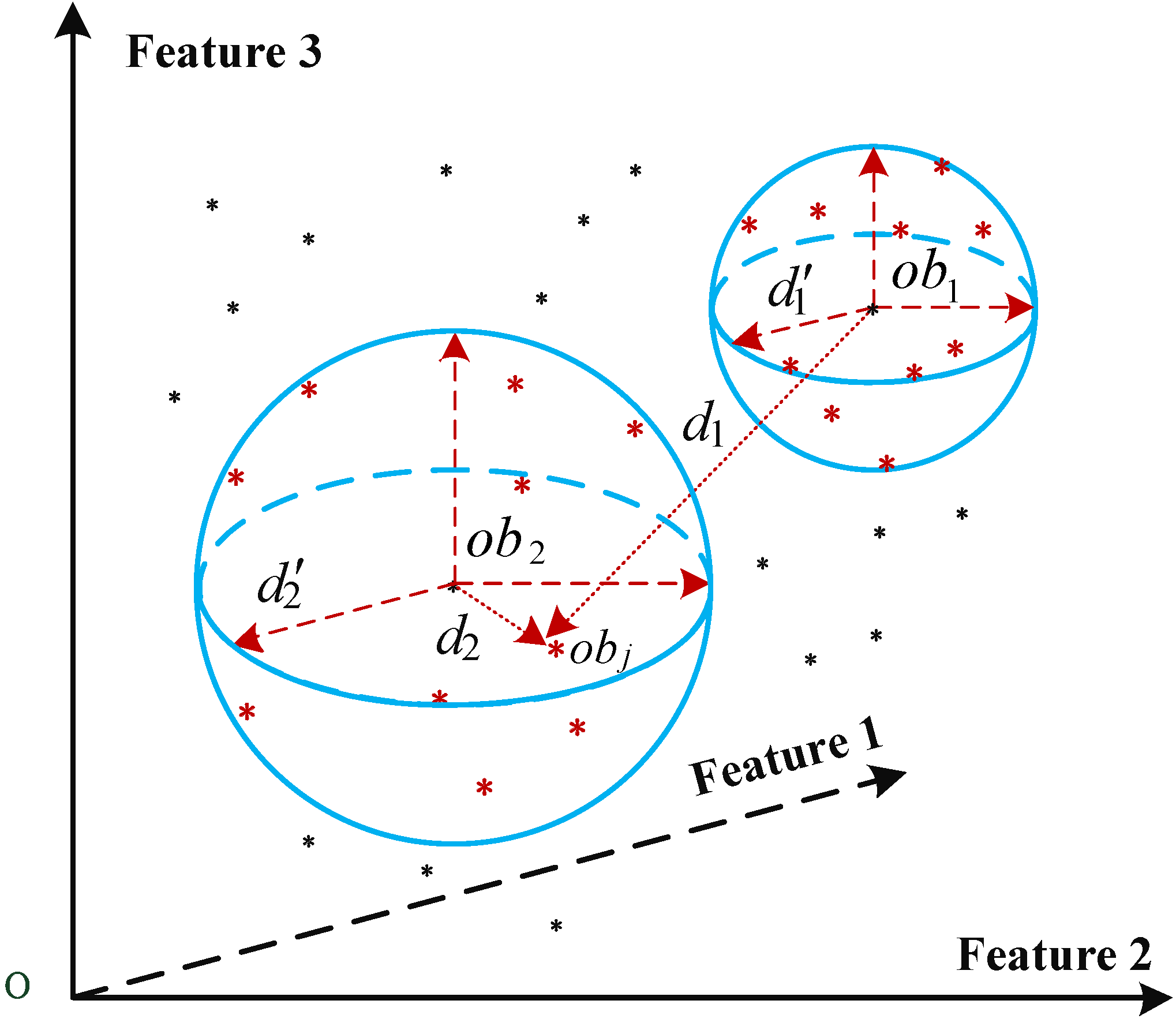
where k is a natural number, and denotes the least number of objects that should be included in the neighborhood of an object. The k_distance denotes the maximum value of Euclidean distance from an object to its neighborhood objects. Let ${\mathrm{N}}_k(o{b}_j)$ be the number of objects in the k_distance neighborhood of object $o{b}_j$, $k\le {\mathrm{N}}_k(o{b}_j)$. $d\left(o{b}_j,o{b}_i\right)$ is the Euclidean distance from object $o{b}_i$ to $o{b}_j$, and $k\_dis\left(o{b}_i\right)$ denotes the k_distance of object $o{b}_i$. The reachability k_distance denotes the maximum value of the k_distance and Euclidean distance from an object to its neighborhood objects. The principle of the reachability 10_distance in three-dimensional texture feature space is shown in Figure 3, where the reachability 10_distance denotes the reachable distance of an object when k value is 10. From Figure 3, the 10_distance of object $o{b}_1$ is $d_1^{\prime }$, and the Euclidean distance from object $o{b}_1$ to $o{b}_j$ is $d_1$. Because $d_1$ is greater than $d_1^{\prime }$, the reachability 10_distance of object $o{b}_1$ with respect to object $o{b}_j$ is $d_1$. By the same reason, the reachability 10_distance of object $o{b}_2$ with respect to object $o{b}_j$ is $d_2^{\prime }$.

The second step is to calculate local reachability density (LRD) of an object according to the reachability distance. Let $\mathrm{LRD}\left(o{b}_j\right)$ be the local reachability density of object $o{b}_j$. $\mathrm{LRD}\left(o{b}_j\right)$ is defined as:

$$\mathrm{LRD}(o{b}_j)=\frac{{\mathrm{N}}_k(o{b}_j)}{{\displaystyle \sum _{i\in {\mathrm{N}}_k(o{b}_j)}{\mathrm{Rdis}}_k(o{b}_j,o{b}_i)}}$$

(7)

$\mathrm{LRD}\left(o{b}_j\right)$ is the inverse of the average reachability distance. Note that $\mathrm{LRD}\left(o{b}_j\right)$ can be $\infty$ if all the reachability distances in the summation are 0.

The last step is to calculate FSOI based on LRD. Let $\mathrm{FSOI}\left(o{b}_j\right)$ be the FSOI of object $o{b}_j$; $\mathrm{FSOI}\left(o{b}_j\right)$ is defined as:

$$\mathrm{FSOI}(o{b}_j)=1-\frac{\mathrm{LRD}(o{b}_j)\times 100\%}{\underset{i\in D}{\max }\left\{\mathrm{LRD}(o{b}_i)\right\}}$$

(8)

where D is the set of objects used for outlier detection. The FSOI value is between 0 and 100%, and the higher its value, the greater the probability that an object deviates from the typical normal objects. Outlier samples and changed objects can be identified according to the size of the FSOI value.

2.2.3. Refining Samples and Selecting the Optimal Texture Features for Each Category

Based on the results of sampling design, changed sample objects can be described as outlier samples in each category. Outlier samples can be identified and eliminated by the iteration of texture feature selection and outlier sample elimination. The iteration procedure can be described as follows:

1.

Calculate the TFCI values using the a priori categories of the initial samples based on Equation (4), and establish the first TFSV by texture feature selection.

2.

Calculate the FSOI values of the initial samples in the TFSV established in step (1) based on Equation (8). Compared with unchanged samples, outlier samples (i.e., the changed samples in the initial sample sets) have higher FSOI values. Thus, outlier samples can be identified by setting an appropriate FSOI threshold. In general, a higher FSOI threshold may misjudge outlier samples as unchanged samples. On the contrary, a lower FSOI threshold may misjudge unchanged samples as outlier samples. In outlier sample detection, it is crucial that all outlier samples must be able to be identified. Accordingly, it is reasonable that each outlier sample can be identified by setting a relatively lower FSOI threshold. Then, eliminate outlier samples by comparing the size of FSOI values with the FSOI threshold, and update sample sets.

3.

Calculate TFCI values using the updated samples in step (2) based on Equation (4), and establish the second TFSV by texture feature selection.

4.

Calculate the FSOI values of samples in the TFSV established in step (3) based on Equation (8). Detect and eliminate outlier samples, and update sample sets.

5.

Repeat steps (3) and (4) until the results of texture feature selection are the same for each category in the last two iterations.

After the iteration, the optimal texture features of each category can be determined, and the samples with unchanged categories can be obtained. Refined samples can be applied to detect changed objects and classify resegmented changed image objects.

2.3. Changed Object Detection Based on the FSOI

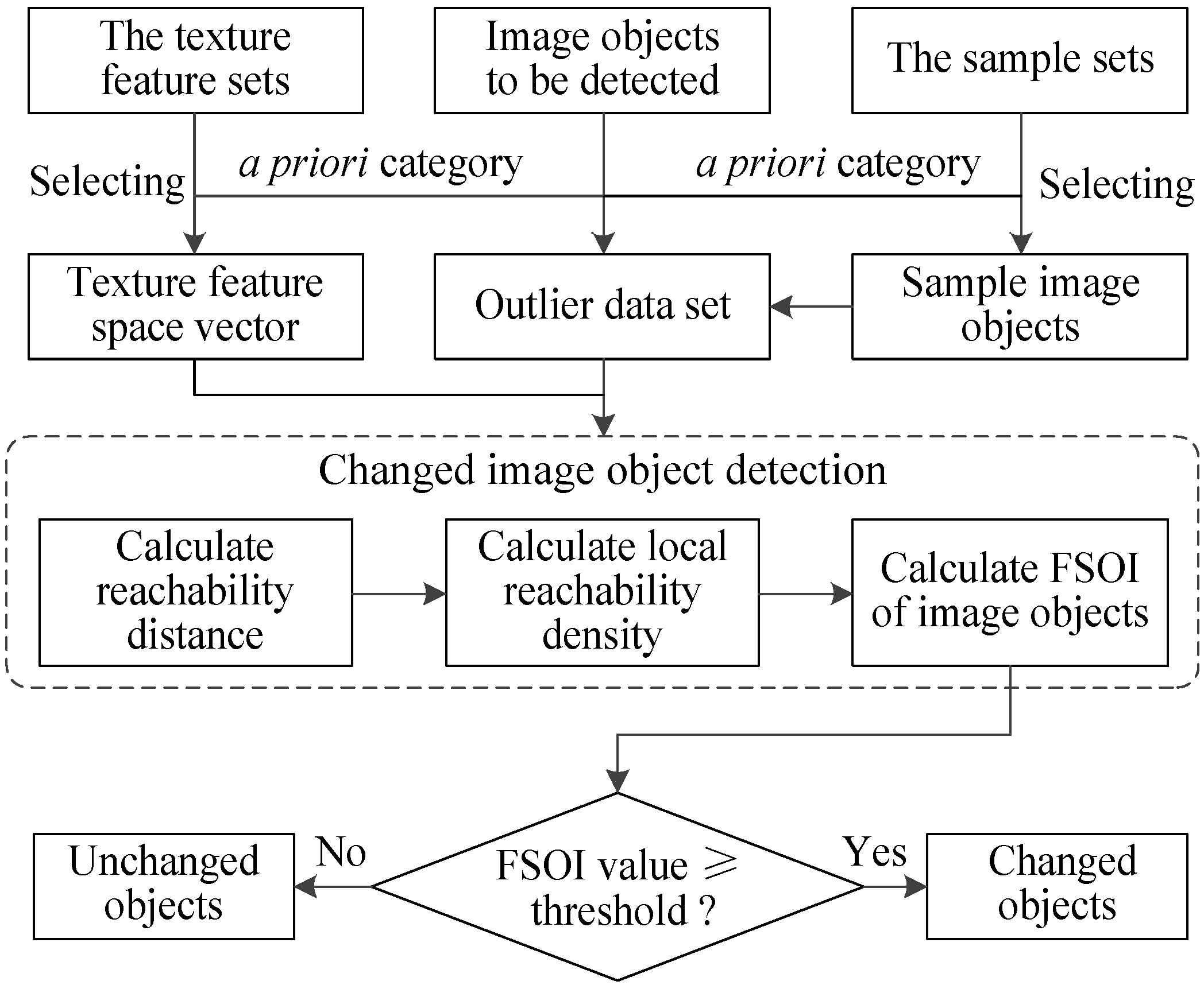
In the proposed texture outlier detection method, changed image objects are considered as outlier data according to texture homogeneity of the refined sample image objects with the same a priori categories. Accordingly, changed objects can be identified with the refined samples by calculating the FSOI values of image objects. Figure 4 presents the process of changed object detection using a texture feature space outlier index. The steps are described in detail as follows.

1.

First, according to the a priori category $c_j$ of an image object to be detected, the data set used for outlier detection with the samples $Sa{m}_j$ and the object $o{b}_i$ is established, and the ${\mathrm{TFSV}}_j$ is determined by the optimal texture features. Let S be the data set used for outlier detection. S can be written as:

$$S=\#\{o{b}_i,Sa{m}_j^1,Sa{m}_j^2,\cdots ,Sa{m}_j^t\}$$

(9)

where $\#\left\{\right\}$ denotes the set of objects used for outlier detection, and t is the number of samples with the same categories $c_j$.

2.

Second, the reachability distance between image objects in S is calculated in the ${\mathrm{TFSV}}_j$ based on Equation (6).

3.

Third, the local reachability density of the image objects in S is calculated by Equation (7).

4.

Then, the FSOI value of the image object $o{b}_i$ can be achieved based on Equation (8). Compared with unchanged image objects, changed image objects have higher FSOI values. Thus, changed image objects can be identified by setting an appropriate FSOI threshold.

5.

Finally, a determination is made whether the object $o{b}_i$ has changed or not by comparing the FSOI value of the object $o{b}_i$ with FSOI threshold. If the FSOI value of the object $o{b}_i$ is greater than FSOI threshold, the object $o{b}_i$ should be identified as changed objects. On the contrary, if the FSOI value of the object $o{b}_i$ is smaller than FSOI threshold, the object $o{b}_i$. should be identified as unchanged objects.

It should be noted that it is necessary and different from outlier sample detection to evaluate results according to overall accuracies for change detection. Both higher and lower FSOI thresholds can reduce the overall accuracy of change detection results. Accordingly, it is very important to set an appropriate FSOI threshold for change detection. In addition, due to partly changing or changing to multiple different objects, the changed image objects must be resegmented to extract change information. Multi-resolution segmentation technology [46,47] is employed to resegment the changed image objects. After resegmenting the changed image objects, the resegmented changed image objects can be classified with the refined samples based on the proposed outlier detection method.

3. Experiments and Results

Since temporal and spatial resolutions, remote sensing sensors, and environmental characteristics have a significant impact on spectral characteristics of surface objects, two study areas are selected to validate the effectiveness and the adaptability of the proposed change detection method, including three experiments using vector data and remote sensing images acquired from different sensors at different times. In addition, the change detection methods based on two-temporal images are also selected to compare with the proposed method.

3.1. Study Areas and Data

3.1.1. Study Area A

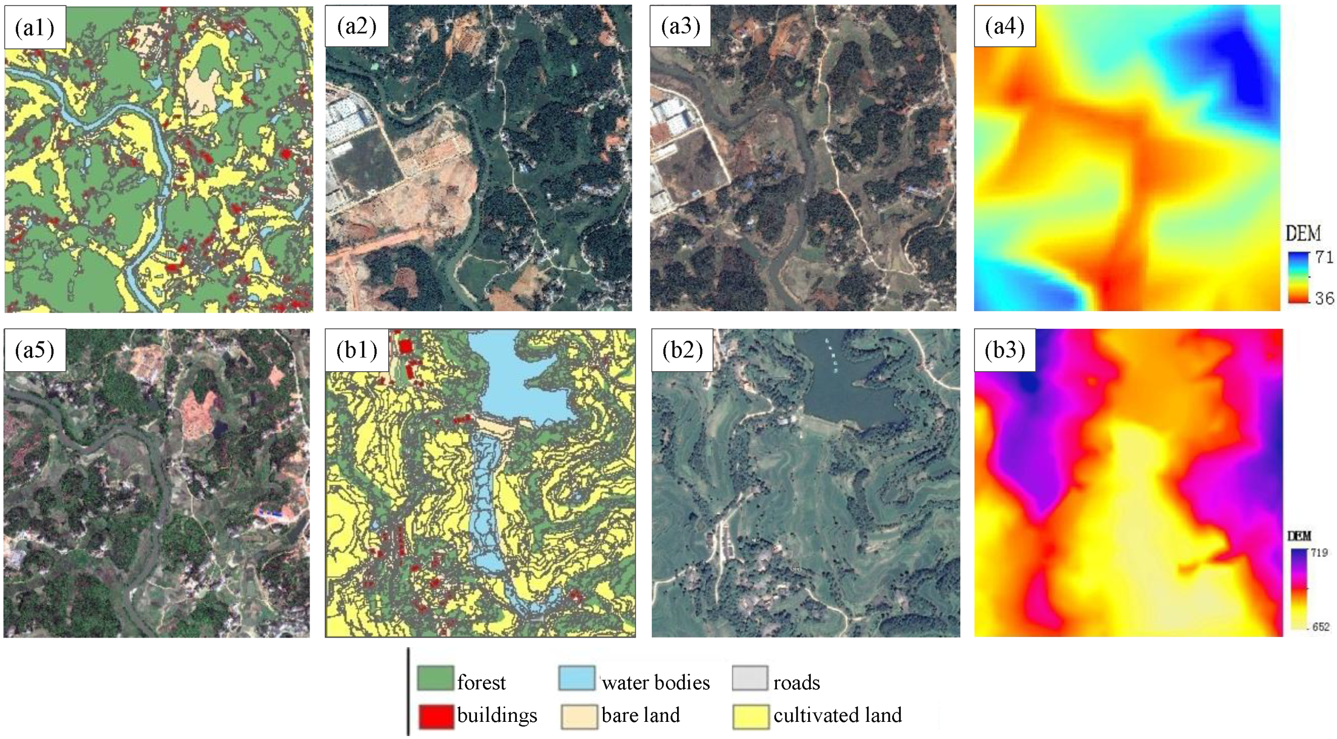
Study area A is located in Miluo City, Hunan province, China (28°29′ N, 113°01′ E). Miluo City is hilly, and the highest and lowest elevations are 71 m and 36 m, respectively (Figure 5(a4)). The experiment data in the study area A include QuickBird images, aerial images, vector data, and DEM. The vector data and DEM were both acquired by digital surveying and mapping in March 2009. The vector data contain 2354 objects and 6 types of surface objects: forest, water bodies, buildings, cultivated land, roads, and bare land (Figure 5(a1)). QuickBird images were acquired on 18 September 2017 (Figure 5(a2)) and 20 April 2009 (Figure 5(a5)), respectively. The size of the QuickBird images is 2920 × 2920 pixels with red, green, and blue bands selected for the experiment, and the spatial resolution of the images is 0.61 m. The size of the aerial images acquired on 8 February 2016 with DOM sensor is 2227 × 2227 pixels with red, green, and blue bands selected for the experiment, and its spatial resolution is 0.8 m (Figure 5(a3)). Two experiments were conducted in the study area A. The QuickBird images on 18 September 2017 and the vector data in March 2009 were used in experiment one, and the aerial images on 8 February 2016 and the vector data in March 2009 were used in experiment two. In addition, the two-temporal QuickBird images on 18 September 2017 and 20 April 2009 were used in the experiment of the change detection methods based on two-temporal images for comparison with the proposed method.

3.1.2. Study Area B

To evaluate the effectiveness of the proposed method in the other study area, another study area B was also selected for experiment three. The study area B is located in Pingchang county, Sichuan province, China (31°30′ N, 106°24′ E). It is a very mountainous region, and its highest and lowest elevations are 712 m and 652 m, respectively (Figure 5(b3)). QuickBird images and vector data were also used in this experiment. The vector data and DEM were both acquired by digital surveying and mapping in April 2014. The vector data contain 1954 objects and 6 types of surface objects (i.e., forest, water bodies, buildings, cultivated land, roads, and bare land (Figure 5(b1)). The QuickBird images were acquired on 14 August 2016 (Figure 5(b2)). The size of the QuickBird images is 2334 × 2334 pixels with red, green, and blue bands selected for the experiment, and the spatial resolution of the images is 0.61 m.

3.2. Results

In the experiments, image objects are first extracted by segmenting images with the vector map. Second, texture features of image objects are calculated according to GLCM. To obtain GLCM of image objects, gray value of each pixel should be calculated by the equal-weighted average of red, green, and blue bands. Third, sampling design is conducted. Then, changed samples are refined by the iteration procedure of texture feature selection and outlier sample detection. Finally, change detection and validation are carried out. In this section, change detection results are thoroughly analyzed, including sampling design, texture feature selection and outlier sample detection, change detection, and validation.

3.2.1. Results of Sampling Design

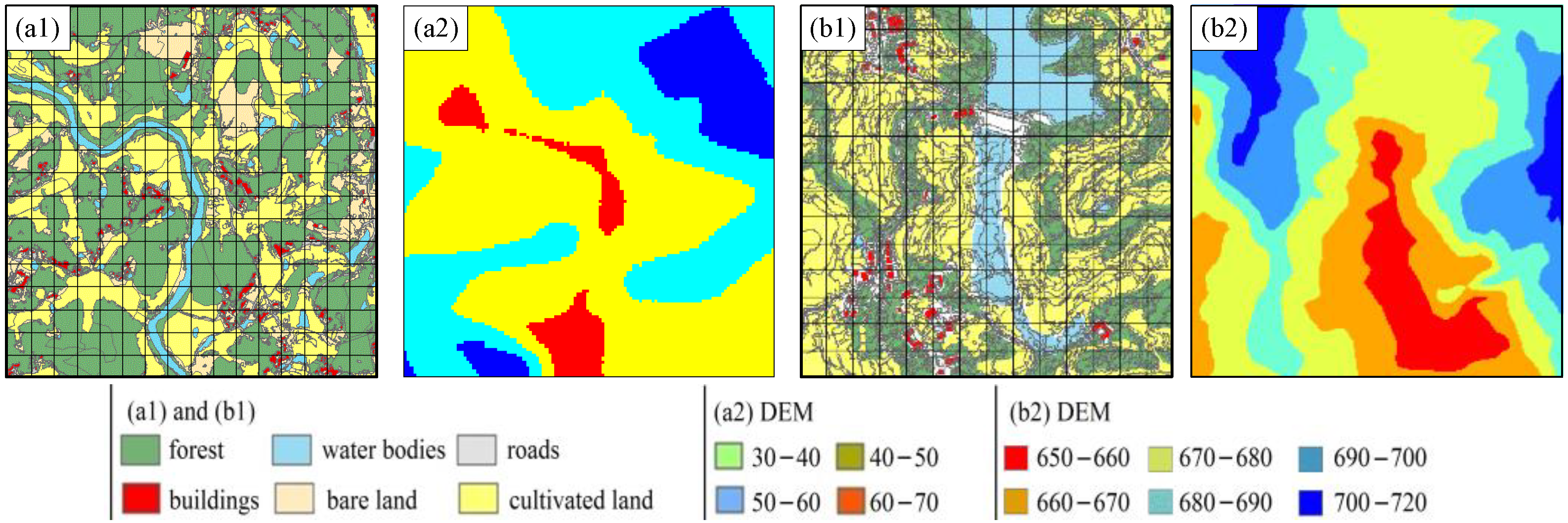
Sampling design needs to be conducted in the study area A and B. The results of sampling design in the study area A are used for the experiments one and two, and the results of sampling design in the study area B are used for the experiment three. According to the proposed sampling design approach, a priori information in the vector map (e.g., spatial distribution of the surface objects and topographic properties in the study area) is employed to allocate samples. First, the sampling area is divided into a uniform grid whose interval is 100 m × 100 m based on horizontal distance. The results of the uniform grids in the study area A and B are shown in Figure 6(a1,b1), respectively. Second, the sampling area is divided into different sampling levels by using the 10 m contour interval as the standard according to topographic properties based on the DEM. The study area A and B is divided into four and six sampling levels, respectively. The results are shown in Figure 6(a2,b2). Then, the number of sampling for six types of surface objects is calculated in each cell according to Equation (1). Finally, sample objects in each cell are distributed in a purely random fashion. The results of the sampling design in the two study areas are shown in Figure 7.

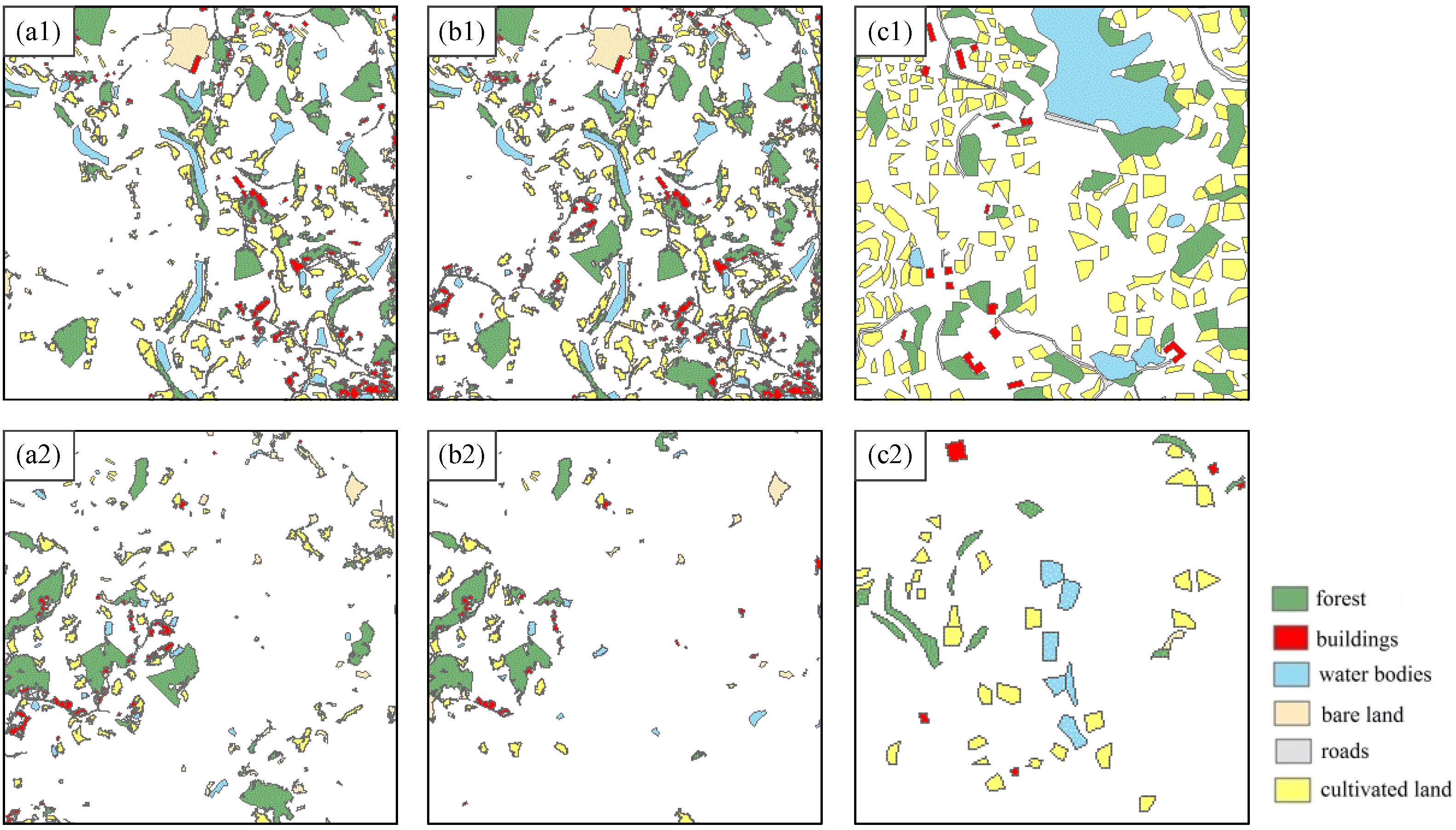
Figure 7(a1,b) are the sample objects for six types of surface objects from the vector map in the study area A and B, respectively. Figure 7(a2,a3) are the sample image objects from the QuickBird images in 2017 and the aerial images in 2016 in the study area A, respectively. It is noted that the sample image objects in the study area B are not shown in Figure 7. Because the sample objects are taken based on a priori information in the vector map, the image objects that have changed in a posteriori category are inevitably sampled. For example, as shown in Figure 7(a2,a3), some changed objects are contained in the sample image objects, and the same results of the sampling design contain a different number of changed samples. However, the number of changed sample objects is smaller than the number of unchanged sample objects. Therefore, the results of sampling design can meet requirements for outlier data.

3.2.2. Texture Feature Selection and Outlier Sample Detection

After obtaining the results of sampling design in the two study areas, the sample image objects need to be refined to eliminate outlier samples and select the optimal features for six types of surface objects in the three experiments. To achieve omission errors of zero in the outlier sample detection, the FSOI threshold and the k value are set as 70% and 1/5 of total number of outlier detection data, respectively, and only the texture features with high and very high contribution levels are selected in the iterations. The sizes of the optimal FSOI threshold and the k value for outlier detection will both be discussed in detail in the discussion section. After the iterations are completed, the results of texture feature selection for six types of surface objects in the three experiments are shown in

Table 3. The results of texture feature selection for six types of surface objects in the three experiments.

Types	Experiment One						Experiment Two						Experiment Three
	Texture Features						Texture Features						Texture Features
	TFCI (%)						TFCI (%)						TFCI (%)
Forest	f6	f9	f8	f4	f1		f6	f8	f9	f1	f3	f4	f3	f2	f12
	100	100	89	85	81		100	100	100	75	75	71	100	86	79
Water bodies	f3	f11	f1	f11			f3	f11					f12	f2	f11
	100	82	72	82			100	85					100	82	76
Buildings	f1	f4					f4	f1					f13	f11	f14
	86	81					91	86					100	64	64
Cultivated land	f6	f9	f8	f7	f2	f10	f3	f11	f6	f8	f9		f6	f9	f8	f1
	100	100	97	93	80	80	100	88	71	71	71		100	100	89	67
Roads	f8	f6	f9				f6	f8	f9				f6	f8	f9
	100	98	98				100	100	100				100	100	100
Bare land	f6	f9	f8				f8	f6	f9				f6	f8	f9
	100	100	98				100	97	97				100	100	100

, and the results of outlier sample detection in the three experiments are shown in Figure 8.

From Table 3, it can be seen that the results of texture feature selection for roads and bare land are both the same or very similar in the three experiments, e.g., f₆, f₈, and f₉ for roads and bare land. Texture features of buildings and water bodies both have similar contribution levels in the same study areas. For example, f₁ and f₄ have high contribution levels on buildings in study area A. However, the results of texture feature selection for cultivated land and forest are both different in the three experiments, and this is mainly due to the different textures of forest and cultivated land caused by different phenological characteristics during different seasons. It follows that selecting the type of texture features is mainly related to textures of the surface objects themselves, but is not strongly related to time, remote sensors, and geographical regions of acquired images. Due to the different textures of the surface objects in different seasons and geographical regions, it is important to select the optimal features for different types of surface objects according to images.

An accuracy assessment is carried out to confirm the effect of outlier samples detection, including commission errors, omission errors, and overall accuracies. In this study, commission errors are defined as the proportion of unchanged objects being judged to be outlier objects in all objects, omission errors are defined as the proportion of changed objects being judged to be normal objects in all objects, and overall accuracies are defined as the proportion of sample objects being correctly identified in all objects. The results of accuracy assessment for six types of surface objects in the three experiments are shown in

Table 4. The accuracies of outlier sample detection for six types of surface objects in the three experiments.

Type	Experiment One			Experiment Two			Experiment Three
	Omission Errors (%)	Commission Errors (%)	Overall Accuracy (%)	Omission Errors (%)	Commission Errors (%)	Overall Accuracy (%)	Omission Errors (%)	Commission Errors (%)	Overall Accuracy (%)
Forest	0	0	100	0	4	96	0	0	100
Buildings	0	0	100	0	0	100	0	5	95
Roads	0	16	84	0	12	88	0	14	86
Water bodies	0	8	92	0	7	93	0	0	100
Bare land	0	19	81	0	18	82	0	8	92
Cultivated land	0	6	94	0	0	100	0	2	98

. It can be seen that omission errors of samples for all types are all 0 in the three experiments, and overall accuracies are all very high. This shows that the results of outlier sample detection can meet the requirements of sample objects used for change detection, and the outlier samples detection approach is effective for samples taken.

3.2.3. Change Detection and Validation

In the two study areas, three experiments were conducted to detect whether or not the objects have changed, respectively. First, image objects with a priori information are extracted from three images using a vector map, respectively. Second, the optimal texture features are selected to establish the TFSV according to a priori categories of image objects, and the data set used for outlier detection is constructed with image objects needed to be detection and sample image objects which have the same a priori categories. Then, the FSOI value of the image object needed to be detection is calculated by Equation (8). In order to obtain higher overall accuracies, FSOI threshold is set as 80% in the change detection experiment. After that, changed objects can be obtained according to the size of the FSOI values. Figure 9(a1,b1,c1) are the change detection results in the three experiments, respectively. In Figure 9(a1,b1,c1), the white areas denote changed areas. It can be seen that there are both clear changes in the two study areas, and there are greater changes in experiment one than in experiment two and three.

Due to partly changing or changing to multiple different objects, the changed image objects must be resegmented to extract change information. Multi-resolution segmentation technology is employed to resegment the changed image objects, and Figure 9(a2,b2,c2) show the results of resegmentation for the changed image objects in the three experiments, respectively. Then, the changed categories can be extracted according to the proposed outlier detection algorithm, i.e., the object can be identified as this type of surface object if the FSOI values of an object in sample objects of one type of surface object are less than the FSOI threshold. The results are shown in Figure 9(a3,b3,c3), respectively. The change extents and trajectories of each type can be calculated according to the results of the changed categories, and the results are shown in

Table 5. Change matrix of six types of surface objects from 2009 to 2017 in experiment one in the study area A.

Types in 2017 (m2)	Types in 2009 (m2)						Total	Changes in 2017
	Forest	Cultivated Land	Bare Land	Water Bodies	Roads	Buildings		(m2)	%
Forest	837,083	167,831	34,919	7976	4639	9202	1,061,650	−414,256	−28.07
Cultivated land	76,106	447,706	53,150	3814	4459	37,204	622,439	−384,266	−38.17
Bare land	188,669	122,642	59,071	380	1280	24,151	396,193	188,508	90.77
Water bodies	12,922	6312	17,953	131,840	1951	22,787	193,765	30,294	18.53
Roads	115,424	91,192	9587	6259	60,057	57,646	340,165	247,975	268.98
Buildings	245,702	171,022	33,005	13,202	19,804	75,727	558,462	331,745	146.33
Total	1,475,906	1,006,705	207,685	163,471	92,190	226,717	3,172,674

,

Table 6. Change matrix of six types of surface objects from 2009 to 2016 in experiment two in the study area A.

Types in 2016 (m2)	Types in 2009 (m2)						Total	Changes in 2016
	Forest	Cultivated Land	Bare Land	Water Bodies	Roads	Buildings		(m2)	%
Forest	1,258,007	51,013	56,558	0	0	50,198	1,415,776	−60,130	−4.07
Cultivated land	0	821,399	0	11,975	0	10,727	844,101	−162,604	−16.15
Bare land	200,206	45,897	50,292	0	0	20,845	317,240	109,555	52.75
Water bodies	0	21,937	0	135,724	0	0	157,661	−5810	−3.55
Roads	0	20,061	0	15,772	61,415	38,657	135,905	43,715	47.41
Buildings	17,693	46,398	100,835	0	30,775	106,290	301,991	75,274	33.20
Total	1,475,906	1,006,705	207,685	163,471	92,190	226,717	3,172,674

and

Table 7. Change matrix of six types of surface objects from 2014 to 2016 in experiment three in the study area B.

Types in 2016 (m2)	Types in 2014 (m2)						Total	Changes in 2016
	Forest	Cultivated Land	Bare Land	Water Bodies	Roads	Buildings		(m2)	%
Forest	522,527	94,714	0	1223	2693	4998	626,154	73,058	13.21
Cultivated land	14,206	839,465	0	61,932	1963	3366	920,932	−74,078	−7.44
Bare land	4943	4881	78,195	1289	947	1319	91,575	6015	7.03
Water bodies	674	2015	0	164,088	0	733	167,510	−71,787	−29.99
Roads	3851	48,694	3409	10,766	106,950	5810	179,479	64,012	55.44
Buildings	6896	5241	3956	0	2914	22,380	41,386	2780	7.20
Total	553,095	995,010	85,560	239,297	115,467	38,606	2,027,036

, respectively.

From Table 5, it can be seen that six types of surface objects have shifted greatly over the period from 2009 to 2017 in the study area A. In this period, forest and cultivated land decreased by 28.07% and 38.17%, respectively. In contrast, roads, buildings, bare land, and water bodies increased by 268.98%, 146.33%, 90.77%, and 18.53%, respectively. In addition, we can explore the reason for internal conversions between different types from Table 5, e.g., the increase of bare land is mainly caused by the decrease of forest and cultivated land. From Table 6, it can also be seen that roads, buildings, and bare land all increased, and forest, water bodies, and cultivated land all decreased over the period from 2009 to 2016 in the study area A. From Table 7, it can be seen that six types of surface objects have also shifted over the period from 2014 to 2016 in the study area B. For example, water bodies and cultivated land decreased by 29.99% and 7.44%, respectively. In contrast, roads, forest, buildings, and bare land increased by 55.44%, 13.21%, 7.20%, and 7.03%, respectively.

Accuracy assessment is an important part of change detection. The most common accuracy assessment elements include overall accuracy, omission errors, commission errors, and the kappa coefficient. The error matrix is the most common method for accuracy assessment of the change detection results. In order to properly generate an error matrix, 468 objects from the change detection results are randomly selected in the three experiments, respectively. The actual types of objects are compared with the results of change detection, and the accuracies of the change detection results are evaluated by omission errors, commission errors, and overall accuracy. The results of accuracy evaluation are shown in

Table 8. The accuracies of change detection result based on the proposed method in the three experiments.

Type	Experiment One		Experiment Two		Experiment Three
	Omission Errors (%)	Commission Errors (%)	Omission Errors (%)	Commission Errors (%)	Omission Errors (%)	Commission Errors (%)
Forest	3.85	6.25	2.56	5.00	2.13	1.28
Cultivated land	3.53	3.53	2.35	3.49	2.36	2.30
Bare land	3.95	7.59	3.95	8.75	3.92	5.19
Water bodies	3.89	1.33	2.67	0.00	1.30	1.56
Roads	4.11	2.78	6.85	2.86	4.32	2.69
Buildings	5.06	2.59	3.80	1.29	2.62	2.53
Overall accuracy	95.94%		96.36%		96.28%
Kappa coefficient	0.951		0.956		0.953

. As shown in Table 8, change detection results have high accuracy. The overall accuracies in the three experiments are 95.94%, 96.36%, and 96.28%, respectively. Omission and commission errors of six types are all very low in the three experiments. Although the accuracies of bare land are relatively lower compared with other types of surface objects, their accuracies are still very high. This shows that the proposed change detection method is valid and can satisfy the accuracy requirement of change detection. The proposed change detection method can be well suited to a variety of study areas and images acquired from different sensors, which can be feasible for the automated change detection and updating land cover data at a large or global scale.

3.3. Comparison of the Proposed OTO-Based Method with Other Change Detection Methods

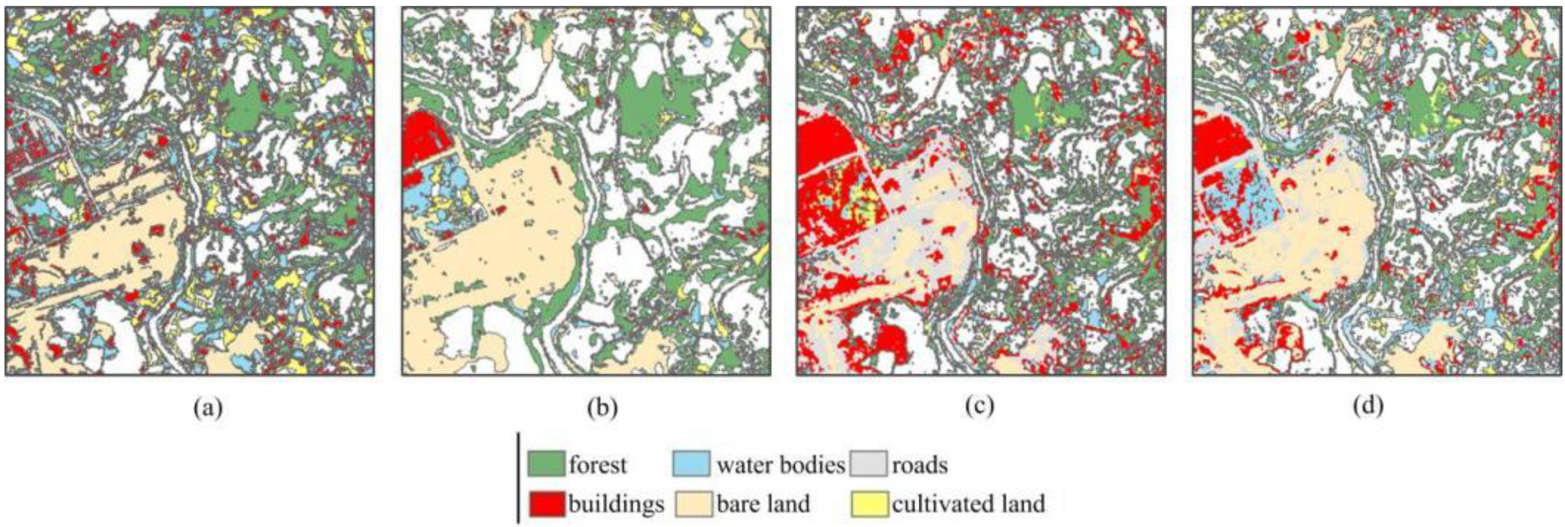
To validate the effectiveness of the proposed method, four other widely used methods based on two-temporal images, e.g., the object-based methods (OBMs) [20], the deep-learning-based methods (DLMs) [26], random forest (RF) [65], and support vector machine (SVM) [24], were selected for comparison. The two-temporal QuickBird images in the study areas A (Figure 5(a2,a5)) are used for experiments. These four change detection methods are all based on the classified images. First, two-temporal images are separately classified into two thematic maps, and then changed results are obtained by implementing comparison of classified images. In the object-based change detection method, remote sensing images are first segmented using the multi-resolution segmentation method from eCognition (v8.7) software, and then the image objects are classified based on the hierarchical classification method. DLM, RF, and SVM all use ENVI (5.3) software to classify two-temporal images and extract change information. The training samples of the four change detection methods required for the supervised classifiers are selected by visual interpretation of images. The change detection results are shown in Figure 10. By visual judgment, there are significant different results of change detection among the four methods. The ground truth data are compared with results of four change detection methods, and the accuracies of change detection results are achieved and are shown in

Table 9. Accuracy of change detection results for four methods.

	Object-Based Methods (OBMs)	Deep-Learning-Based Method (DLMs)	Random Forest (RF)	Support Vector Machine (SVM)	Proposed Method
Overall accuracy (%)	79.23	90.16	78.50	80.50	95.94
Omission errors (%)	9.68	4.12	8.04	9.47	1.87
Commission errors (%)	11.09	5.72	13.46	10.03	2.19

.

As shown in Table 9, the overall accuracies of OBMs, DLMs, RF, and SVM are 79.23%, 90.16%, 78.5%, and 80.5%, respectively. The overall accuracy of the proposed change detection method is higher than that of the four methods. The omission and commission errors of the four methods are all higher than those of the proposed change detection method. Compared with the proposed method, the shortfalls of the four methods mainly include: (1) it is difficult to choose training samples due to the lack of a priori information; (2) the results of change detection are sensitive to the training data quality and the number of training samples; and (3) unchanged areas need to also be classified. In conclusion, the proposed change detection method is outstanding. The main reasons include: (a) using existing vector data to segment images can reduce the search space and minimize false segmentation of objects from images, (b) the change detection error caused by the transmission of classification error is reduced to a great extent, and (c) samples for change detection are taken automatically.

4. Discussion

4.1. Influence of Sample Proportions and Sizes on the Texture Feature Selection of Surface Objects

In the proposed change detection method, it is very important to select the optimal texture features for types of surface objects. However, the optimal texture features need to be identified by calculating TFCI values using samples. Therefore, to test the influence of sample proportions and sizes on the TFCI value, different sampling schemes will be executed in this section.

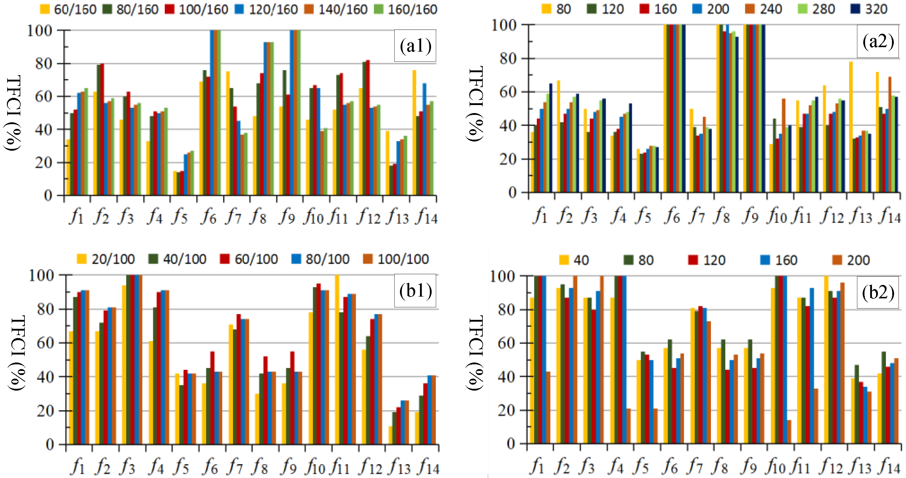
Two types of surface objects from the QuickBird images in the study area B (Figure 5(b2)), i.e., cultivated land and forest, are selected for the experiment. Two sets of experiments for each type of surface objects are designed to test the influence of samples on the TFCI value. The first set of experiments with different sample proportions are carried out to observe the difference of the TFCI value, and the results of TFCI values for cultivated land and forest are shown in Figure 11(a1,b1), respectively. As shown in Figure 11(a1), the size of cultivated land objects included in samples varies from 60 to 160, and the size of the other types of surface objects is fixed as 160. For example, in Figure 11(a1), 60/160 denotes 60 cultivated land objects and 160 other types of surface objects which are included in the samples. As shown in Figure 11(b1), the size of forest objects included in samples varies from 20 to 100, and the size of the other types of surface objects is fixed as 100. For example, in Figure 11(b1), 20/100 denotes 20 forest objects and 100 other types of surface objects which are included in the samples. The second set of experiments with the same sample proportions and different total sample sizes are carried out to observe the difference of the TFCI value, and the results of TFCI values for cultivated land and forest are shown in Figure 11(a2,b2), respectively. As shown in Figure 11(a2), the sample proportions of cultivated land objects are fixed as 50%, and the total sample sizes vary from 80 to 320. As shown in Figure 11(b2), the total sample sizes vary from 40 to 200 when the sample proportions of forest objects are fixed as 50%.

From Figure 11(a1), it can be seen that the contribution levels of texture features on cultivated land are all very similar when the number of cultivated land objects varies from 60 to 160. For example, the TFCI values of f₅ and f₁₃ are both lower than 40%, and it shows that f₅ and f₁₃ are both in low contribution levels. The TFCI values f₆, f₈ and f₉ are all higher than 60%, and they are all in high contribution levels. The same conclusions can also be drawn in Figure 11(b1), e.g., f₁, f₂, f₃, f₄, f₇, f₁₀, f₁₁ and f₁₂ all have high or very high contribution levels on forest. From Figure 11(a2), it can also be seen that f₆, f₈ and f₉ all have very high contribution levels on cultivated land when the total sample sizes vary from 80 to 320. As shown in Figure 11(b2), f₁, f₂, f₃, f₄, f₁₀, f₁₁ and f₁₂ all have very high contribution levels on forest when the total sample sizes vary from 40 to 200. The overall result indicates that contribution levels of texture features on types of surface objects will not be affected by sample proportions and sizes.

4.2. Influence of Image Data Source on the Texture Feature Selection of Surface Objects

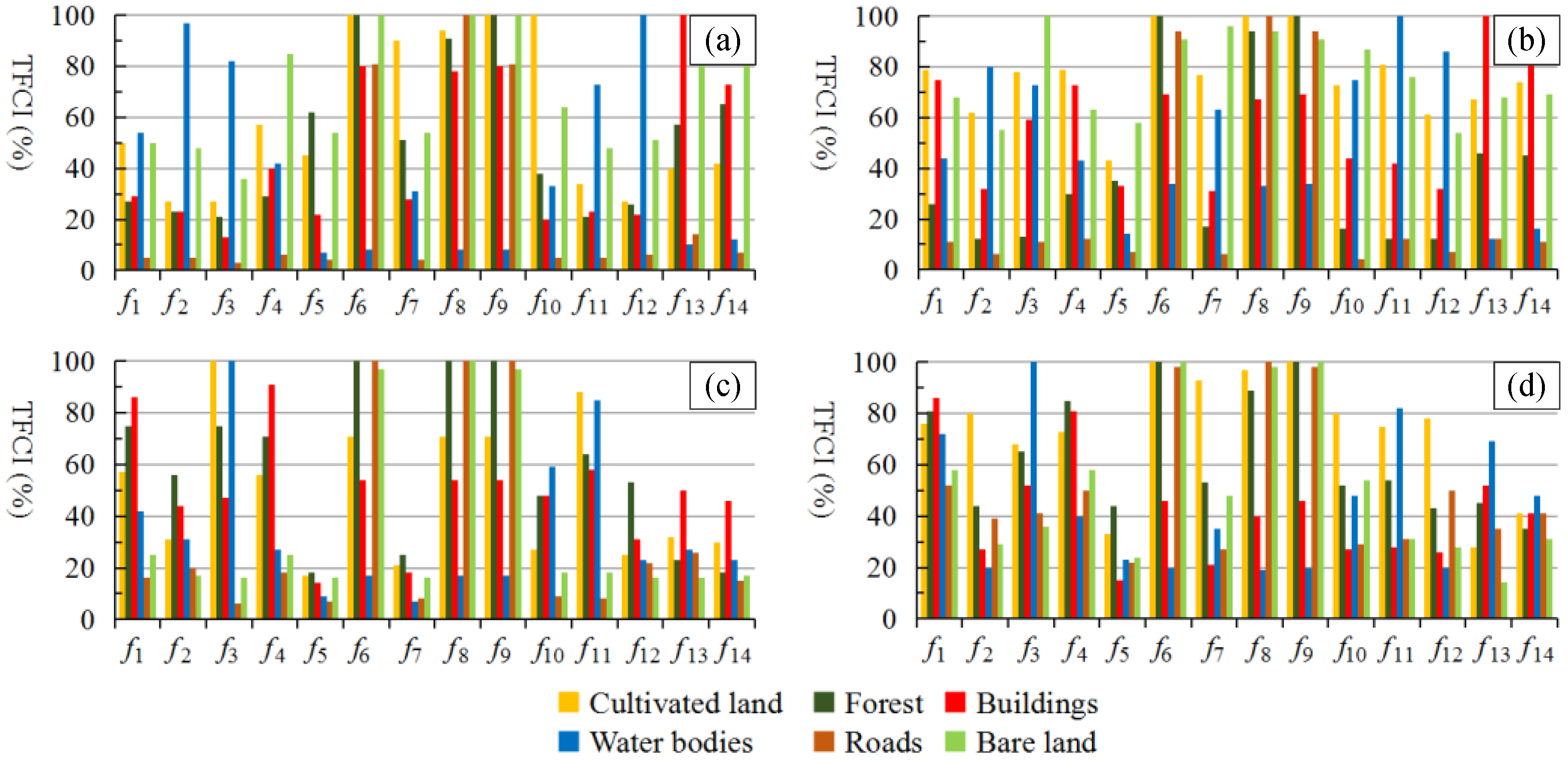
To test the influence of different image data sources on the texture feature selection of surface objects, two study areas including four images are selected for the experiment. The first study area is located in Changsha city, Hunan province, China, including two aerial images with DOM sensor acquired in March 2009 and September 2013, respectively. The spatial resolution of the aerial images is 0.61 m with red, green, and blue bands. Two aerial images are not shown in the figures. The second study area includes two QuickBird images acquired in March 2009 and September 2017, respectively. Two QuickBird images are shown in Figure 5(a2,a5). Six types of surface objects are both included in the two study areas. To compare the results of experiments from different image data sources, 300 samples are selected for experiment in each study area, including 50 samples for each type of surface object. The results of TFCI values of six types of surface objects from four images are shown in Figure 12. Figure 12a,b are the results of TFCI values of six types of surface objects from the aerial images in March 2009 and September 2013, respectively. Figure 12c,d are the results of TFCI values of six types of surface objects from the QuickBird images in March 2009 and September 2017, respectively.

From Figure 12, it can be seen that the contribution levels of some texture features on bare land and roads are very similar in the four images. For example, f₆, f₈ and f₉ all have very high contribution levels on bare land and roads. Texture features of buildings and water bodies both have similar contribution levels in the same study areas, and their contribution levels are different in the different study areas. For example, f₆, f₈, f₉, f₁₃ and f₁₄ all have high contribution levels on buildings in the first study area. f1 and f4 have high contribution levels on buildings in the second study area. However, the contribution levels of texture features on cultivated land and forest are very different in the four images. Thus, it can be seen that the different contribution levels of texture features on types of surface objects are mainly caused by different textures of the surface objects themselves. For example, textures of building roofs are different in different study areas due to different architectural styles, and forest and cultivated land have different textures during different phenological periods.

Therefore, it is very important to select the optimal features for different types of surface objects according to images acquired from different study areas and phenological periods because of the different textures of the surface objects in different seasons and geographical regions.

4.3. Role of Neighborhood Parameter k and FSOI Threshold in Outlier Detection

Calculating the FSOI values of image objects, the only parameter that needs to be set is the neighborhood parameter k. The FSOI value of an image object is affected by the size of k value, owing to the following: the greater the number of image objects included in the neighborhood, the smaller the probability that they belong to the same category. In addition, setting an appropriate FSOI threshold can also remarkably increase the accuracy of outlier detection. Therefore, it is very important to select an appropriate k value and FSOI threshold for outlier detection.

To evaluate the effect of different k values and FSOI threshold on outlier detection, four sets of outlier detection data from the QuickBird images acquired on 18 September 2017 in the study area A (Figure 5(a2)), i.e., cultivated land (145 cultivated land objects and 65 outlier objects), forest (120 forest objects and 30 outlier objects), buildings (85 buildings objects and 35 outlier objects), and water bodies (135 water bodies objects and 45 outlier objects) are selected for experiment. It should be noted that these outlier detection data were randomly selected by visual interpretation, which does not affect the implementation of the proposed automatic change detection.

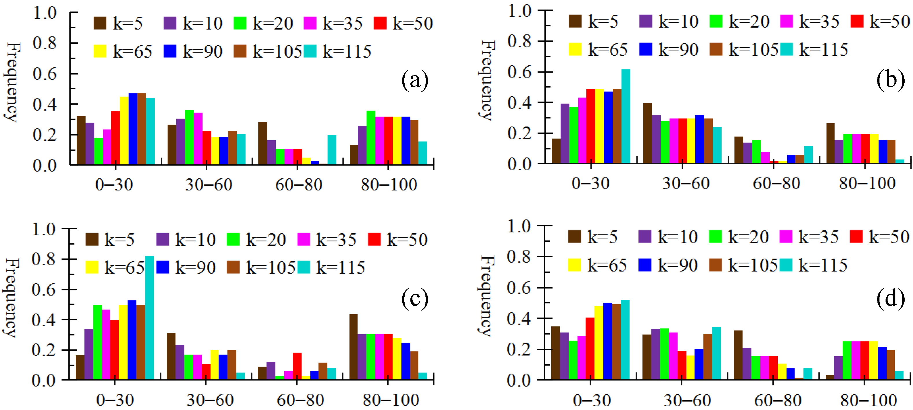
To effectively achieve outlier detection, it is necessary and important to construct a texture feature space vector for the outlier detection data by selecting the optimal texture features. The results of texture features selection for four sets of outlier detection data are shown in Table 3 (experiment one). Then, the FSOI values of each object are calculated, and the frequency distribution histograms of the FSOI values for outlier detection data with different k values are shown in Figure 13. As shown in Figure 13, it is clear that the number of objects at a low FSOI interval increases gradually with the increase of the k value, and the number at the high FSOI interval decreases gradually. When the k value changes during a certain range, e.g., 35–65 in Figure 13a, the number of objects at high FSOI interval tends to be stable. When the k value is too large (e.g., close to the total number of outlier detection data), the objects to be detected are almost all at a low outlier degree level, e.g., Figure 13c. Therefore, a k value that is set too large or too small decreases the accuracy of the outlier detection results, and it is very important to select an appropriate k value for outlier detection. From Figure 13, we can conclude that it is reasonable to set k value as 1/5–1/3 of the number of total outlier detection objects.

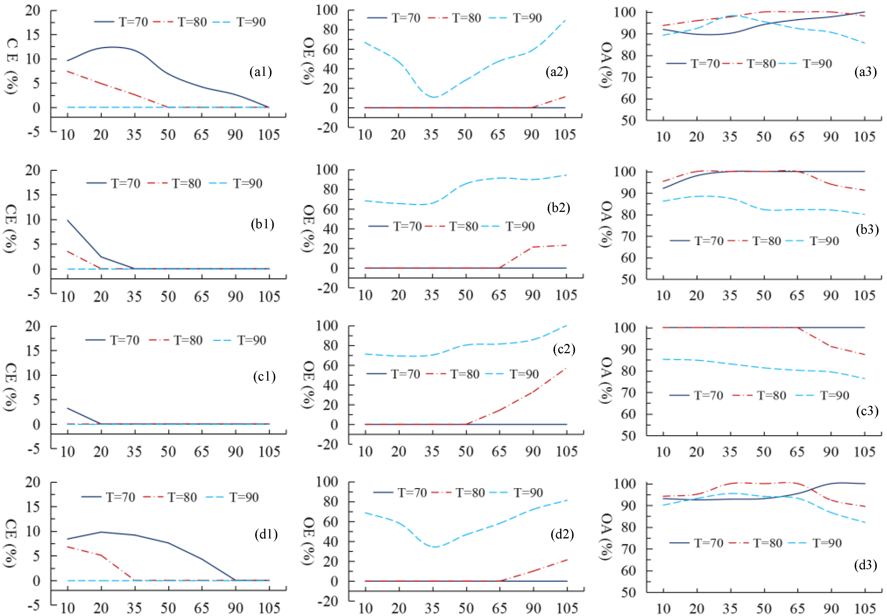
To quantitatively evaluate the effect of outlier detection, commission errors, omission errors, and overall accuracies of four sets of outlier data are calculated by different k values and FSOI threshold, the results of which are shown in Figure 14. As shown in Figure 14, the higher the FSOI threshold, the higher the omission errors and the lower the commission errors, On the contrary, the lower the FSOI threshold, the lower the omission errors, and the higher the commission errors. Omission errors and commission errors can both reach 0, and overall accuracies can all reach 100% when the FSOI threshold is set as 80% and an appropriate k value is selected (e.g., 50–90 in Figure 14(a1–a3), 35–65 in Figure 14(b1–b3), 20–50 in Figure 14(c1–c3), and 35–65 in Figure 14(d1–d3)). When the FSOI threshold is set as 70%, no matter what the value of k is, omission errors can all reach 0; however, that would lead to a high commission error and low overall accuracies. It is reasonable that omission errors can reach 0 at the cost of high commission errors in outlier sample detection, but it is necessary to evaluate the experimental results according to overall accuracies in change detection. Therefore, the results of outlier detection are valid and reliable when the k value is set as 1/5–1/3 of the number of total outlier detection objects and the FSOI threshold is set as 80%.

4.4. Role of Texture Feature Selection in Outlier Detection

In the existing literature, only a few texture features are considered based on experience to describe the texture information of image objects, which lacks accurate quantitative evaluation. For example, Anniballe et al. [66] selected five texture features (contrast, correlation, energy, homogeneity, and entropy) to investigate the textural properties of buildings. However, Sofina and Ehlers et al. [38] utilized three other texture features (angular second moment, contrast, and inverse difference moment) to detect buildings damaged by an earthquake. To evaluate the performance of the optimal texture features on outlier detection, two experiments with and without texture feature selection are conducted. The QuickBird images acquired on 18 September 2017 in the study area A (Figure 5(a2)) are used for two experiments. To compare the results of two experiments, 600 objects are selected in each experiment, including 300 outlier objects (changed objects). The frequency distribution histograms of outlier detection with and without texture feature selection are shown in Figure 15a,b, respectively.

From Figure 15a, it can be seen that the FSOI values of unchanged objects are smaller than 80%, while those of outlier objects (changed objects) are mostly larger than 80%. This indicates that the FSOI values of objects with the optimal texture feature selection can be used to distinguish changed and unchanged objects. However, the distributions of changed and unchanged objects both overlap considerably in Figure 15b. Thus, it is difficult to distinguish changed and unchanged objects based on the FSOI values of objects without optimal texture feature selection. When the FSOI threshold is set as 80%, the results of the quantitative accuracy analysis of the outlier detection with and without texture feature selection are shown in

Table 10. Accuracy of outlier detection with and without texture feature selection.

	Omission Errors (%)	Commission Errors (%)	Overall Accuracy (%)
with texture feature selection	4.52	0.72	94.76
without texture feature selection	35.00	7.22	57.78

. Compared with the optimal texture features, the overall accuracy of outlier detection without texture feature selection, which reduced significantly, is only 57.78%. The omission and commission errors, which both significantly increased, reach 35.00% and 7.22%, respectively. Therefore, the best accuracy results of outlier detection depend on the results of the optimal texture features.

5. Conclusions

In this paper, we have proposed a change detection method using a texture feature space outlier index from mono-temporal remote sensing images and existing vector data. In the proposed method, the vector data are taken as a substitute for historic remote sensing images, and changed objects in the recent images are considered as outlier data according to texture homogeneity among objects belonging to the same category. The sampling design considering spatial distribution and topographic properties of image objects is devised to incorporate as few changed samples as possible while still having enough statistical power to detect changed objects. A TFCI is defined by information gain to select the optimal texture features for each category. An FSOI based on local reachability density is presented to automatically detect outlier samples and changed objects. Samples with changed categories are refined by the iteration procedure of texture feature selection and outlier sample elimination. Overall, the proposed method has the following advantages: (a) the proposed method can reduce the search space and minimize false segmentation of image objects by using existing vector data to segment images, (b) the change detection error caused by the transmission of classification error can be reduced to a great extent, and (c) samples for change detection can be automatically extracted.

The performance of the proposed method was tested by three experiments in the two study areas. In outlier samples detection, omission errors of zero can be achieved when the FSOI threshold is set as 70%. In change detection, overall accuracies of 95.94%, 96.36%, and 96.28% were achieved in the three experiments, respectively, while the omission errors and commission errors of every category were all very low. To validate the effectiveness of the proposed method, four other widely used methods (i.e., OBMs, DLMs, RF, and SVM) based on two-temporal images were used for comparison. The experiment results showed that the accuracy of the proposed method is higher than that of the four change detection methods.

The proposed method can be well suited to a variety of images and different study areas, can accurately detect a given geographical object, and can be applied for ecological environmental monitoring, spatial data updating, and post-disaster emergencies, etc. Despite the advantages in our method, much work remains to improve the effectiveness of change detection from mono-temporal images. For example, the FSOI threshold plays an important role in detecting changed objects by the proposed outlier detection technique, but it is set though many experiments in this paper. Therefore, future work will investigate how to set the FSOI threshold with a more reasonable approach. In addition, our proposed method may not be efficient and accurate for change detection of high-rise buildings in city areas, because it is often inaccurate in identifying high-rise building roofs from an image by using a vector map.

References

1. Wu, C.; Du, B.; Zhang, L. Hyperspectral anomalous change detection based on joint sparse representation. ISPRS J. Photogramm. Remote Sens. 2018, 146, 137–150. [Google Scholar] [CrossRef]
2. Coppin, P.; Jonckheere, I.; Nackaerts, K.; Muys, B.; Lambin, E. Review ArticleDigital change detection methods in ecosystem monitoring: A review. Int. J. Remote Sens. 2004, 25, 1565–1596. [Google Scholar] [CrossRef]
3. Singh, A. Digital change detection techniques using remotely sensed data. Int. J. Remote Sens. 1988, 10, 989–1003. [Google Scholar] [CrossRef] [Green Version]
4. Chen, J.; Chen, J.; Liao, A.; Cao, X.; Chen, L.; Chen, X.; He, C.; Han, G.; Peng, S.; Lu, M.; et al. Global land cover mapping at 30 m resolution: A POK-based operational approach. ISPRS J. Photogramm. Remote Sens. 2015, 103, 7–27. [Google Scholar] [CrossRef] [Green Version]
5. Sterling, S.M.; Ducharne, A.; Polcher, J. The impact of global land-cover change on the terrestrial water cycle. Nat. Clim. Chang. 2012, 3, 385–390. [Google Scholar] [CrossRef]
6. Foley, J.A.; DeFries, R.; Asner, G.; Barford, C.; Bonan, G.; Carpenter, S.R.; Chapin, F.S.; Coe, M.; Daily, G.C.; Gibbs, H.K.; et al. Global Consequences of Land Use. Science 2005, 309, 570–574. [Google Scholar] [CrossRef] [PubMed] [Green Version]
7. Bruzzone, L.; Serpico, S. An iterative technique for the detection of land-cover transitions in multitemporal remote-sensing images. IEEE Trans. Geosci. Remote Sens. 1997, 35, 858–867. [Google Scholar] [CrossRef] [Green Version]
8. Lambin, E.F.; Ehrlich, D. Land-cover changes in sub-saharan Africa (1982–1991): Application of a change index based on remotely sensed surface temperature and vegetation indices at a continental scale. Remote Sens. Environ. 1997, 61, 181–200. [Google Scholar] [CrossRef]
9. Varma, S.; Shah, V.; Banerjee, B.; Buddhiraju, K.M. Change Detection of Desert Sand Dunes: A Remote Sensing Approach. Adv. Remote Sens. 2014, 3, 10–22. [Google Scholar] [CrossRef] [Green Version]
10. Chen, X.; Chen, J.; Shi, Y.; Yamaguchi, Y. An automated approach for updating land cover maps based on integrated change detection and classifi-cation methods. ISPRS J. Photogramm. Remote Sens. 2012, 71, 86–95. [Google Scholar] [CrossRef]
11. Rogan, J.; Chen, D. Remote sensing technology for mapping and monitoring land-cover and land-use change. Prog. Plan. 2004, 61, 301–325. [Google Scholar] [CrossRef]
12. Hussain, M.; Chen, D.; Cheng, A.; Wei, H.; Stanley, D. Change detection from remotely sensed images: From pixel-based to object-based approaches. ISPRS J. Photogramm. Remote Sens. 2013, 80, 91–106. [Google Scholar] [CrossRef]
13. Lu, D.; Mausel, P.; Brondizio, E.; Moran, E. Change detection techniques. Int. J. Remote Sens. 2004, 25, 2365–2401. [Google Scholar] [CrossRef]
14. Alphan, H.; Derse, M.A. Change detection in Southern Turkey using normalized difference vegetation index (NDVI). J. Environ. Eng. Landsc. Manag. 2012, 21, 12–18. [Google Scholar] [CrossRef]
15. Bovolo, F.; Bruzzone, L. A Theoretical Framework for Unsupervised Change Detection Based on Change Vector Analysis in the Polar Domain. IEEE Trans. Geosci. Remote Sens. 2006, 45, 218–236. [Google Scholar] [CrossRef] [Green Version]
16. FAN, H.; MA, A.; LI, J. Case Study on Image Differencing Method for Land Use Change Detection Using Thematic Data in Renhe District of Panzhi-hua. J. Remote Sens. 2001, 5, 75–80. [Google Scholar]
17. Townshend, J.R.G.; Justice, C.O. Spatial variability of images and the monitoring of changes in the Normalized Difference Vegetation Index. Int. J. Remote Sens. 1995, 16, 2187–2195. [Google Scholar] [CrossRef]
18. Alphan, H.; Doygun, H.; Unlukaplan, Y.I. Post-classification comparison of land cover using multitemporal Landsat and ASTER imagery: The case of Kahramanmaraş, Turkey. Environ. Monit. Assess. 2008, 151, 327–336. [Google Scholar] [CrossRef] [PubMed]
19. Manandhar, R.; Odeh, I.O.A.; Ancev, T. Improving the Accuracy of Land Use and Land Cover Classification of Landsat Data Using Post-Classification Enhancement. Remote Sens. 2009, 1, 330–344. [Google Scholar] [CrossRef] [Green Version]
20. Dronova, I.; Gong, P.; Wang, L. Object-based analysis and change detection of major wetland cover types and their classification uncertainty during the low water period at Poyang Lake, China. Remote Sens. Environ. 2011, 115, 3220–3236. [Google Scholar] [CrossRef]
21. Vidal, A.; Moreno, M.R. Change detection of isolated housing using a new hybrid approach based on object classification with optical and Ter-raSAR-X data. Int. J. Remote Sens. 2011, 32, 9621–9635. [Google Scholar] [CrossRef] [Green Version]
22. Duro, D.; Franklin, S.; Dubé, M. Hybrid Object-based Change Detection and Hierarchical Image Segmentation for Thematic Map Updating. Photogramm. Eng. Remote Sens. 2013, 79, 259–268. [Google Scholar] [CrossRef]
23. Eisavi, V.; Homayouni, S. Performance evaluation of random forest and support vector regressions in natural hazard change detection. J. Appl. Remote Sens. 2016, 10, 46030. [Google Scholar] [CrossRef]
24. Cao, G.; Li, Y.; Liu, Y.; Shang, Y. Automatic change detection in high-resolution remote-sensing images by means of level set evolution and support vector machine classification. Int. J. Remote Sens. 2014, 35, 6255–6270. [Google Scholar] [CrossRef]
25. Woodcock, C.; Macomber, S.; Pax-Lenney, M.; Cohen, W.B. Monitoring large areas for forest change using Landsat: Generalization across space, time and Landsat sensors. Remote Sens. Environ. 2001, 78, 194–203. [Google Scholar] [CrossRef] [Green Version]
26. De, S.; Pirrone, D.; Bovolo, F.; Bruzzone, L.; Bhattacharya, A. A novel change detection framework based on deep learning for the analysis of mul-ti-temporal polarimetric SAR images. In Proceedings of the 2017 IEEE International Geoscience and Remote Sensing Symposium (IGARSS), Fort Worth, TX, USA, 23–28 July 2017; pp. 5193–5196. [Google Scholar]
27. Zhang, P.; Gong, M.; Su, L.; Liu, J.; Li, Z. Change detection based on deep feature representation and mapping transformation for mul-ti-spatial-resolution remote sensing images. ISPRS J. Photogramm. Remote Sens. 2016, 116, 24–41. [Google Scholar] [CrossRef]
28. Bouziani, M.; Goïta, K.; He, D.-C. Automatic change detection of buildings in urban environment from very high spatial resolution images using exist-ing geodatabase and prior knowledge. ISPRS J. Photogramm. Remote Sens. 2010, 65, 143–153. [Google Scholar] [CrossRef]
29. Bayarjargal, Y.; Karnieli, A.; Bayasgalan, M.; Khudulmur, S.; Gandush, C.; Tucker, C. A comparative study of NOAA–AVHRR derived drought indi-ces using change vector analysis. Remote Sens. Environ. 2006, 105, 9–22. [Google Scholar] [CrossRef]
30. Nackaerts, K.; Vaesen, K.; Muys, B.; Coppin, P. Comparative performance of a modified change vector analysis in forest change detection. Int. J. Remote Sens. 2005, 26, 839–852. [Google Scholar] [CrossRef]
31. Ghosh, A.; Mishra, N.S.; Ghosh, S. Fuzzy clustering algorithms for unsupervised change detection in remote sensing images. Inf. Sci. 2011, 181, 699–715. [Google Scholar] [CrossRef]
32. Yuan, F.; Sawaya, K.E.; Loeffelholz, B.C.; Bauer, M.E. Land cover classification and change analysis of the Twin Cities (Minnesota) Metropolitan Area by multitemporal Landsat remote sensing. Remote Sens. Environ. 2005, 98, 317–328. [Google Scholar] [CrossRef]
33. Habib, T.; Inglada, J.; Mercier, G.; Chanussot, J. Support Vector Reduction in SVM Algorithm for Abrupt Change Detection in Remote Sensing. IEEE Geosci. Remote Sens. Lett. 2009, 6, 606–610. [Google Scholar] [CrossRef]
34. Huang, C.; Song, K.; Kim, S.; Townshend, J.R.; Davis, P.; Masek, J.G.; Goward, S.N. Use of a dark object concept and support vector machines to automate forest cover change analysis. Remote Sens. Environ. 2008, 112, 970–985. [Google Scholar] [CrossRef]
35. Zhang, H.; Gong, M.; Zhang, P.; Su, L.; Shi, J. Feature-Level Change Detection Using Deep Representation and Feature Change Analysis for Multispectral Imagery. IEEE Geosci. Remote Sens. Lett. 2016, 13, 1666–1670. [Google Scholar] [CrossRef]
36. Gong, M.; Zhao, J.; Liu, J.; Miao, Q.; Jiao, L. Change Detection in Synthetic Aperture Radar Images Based on Deep Neural Networks. IEEE Trans. Neural Netw. Learn. Syst. 2016, 27, 125–138. [Google Scholar] [CrossRef] [PubMed]
37. Zhu, Z. Change detection using landsat time series: A review of frequencies, preprocessing, algorithms, and applications. ISPRS J. Photogramm. Remote Sens. 2017, 130, 370–384. [Google Scholar] [CrossRef]
38. Sofina, N.; Ehlers, M. Building Change Detection Using High Resolution Remotely Sensed Data and GIS. IEEE J. Sel. Top. Appl. Earth Obs. Remote Sens. 2016, 9, 3430–3438. [Google Scholar] [CrossRef]
39. Guo, Z.; Du, S. Mining parameter information for building extraction and change detection with very high-resolution imagery and GIS data. GIScience Remote Sens. 2016, 54, 38–63. [Google Scholar] [CrossRef]
40. Hegazy, I.R.; Kaloop, M.R. Monitoring urban growth and land use change detection with GIS and remote sensing techniques in Daqahlia governorate Egypt. Int. J. Sustain. Built Environ. 2015, 4, 117–124. [Google Scholar] [CrossRef] [Green Version]
41. Li, D. Remotely sensed images and GIS data fusion for automatic change detection. Int. J. Image Data Fusion 2010, 1, 99–108. [Google Scholar] [CrossRef]
42. Baltsavias, E. Object extraction and revision by image analysis using existing geodata and knowledge: Current status and steps towards operational systems. ISPRS J. Photogramm. Remote Sens. 2004, 58, 129–151. [Google Scholar] [CrossRef]
43. Turker, M.; Cetinkaya, B. Automatic detection of earthquake-damaged buildings using DEMs created from pre-and post-earthquake stereo aerial photographs. Int. J. Remote Sens. 2005, 26, 823–832. [Google Scholar] [CrossRef]
44. De Alwis, D.A.; So, E. Enhanced change detection index for disaster response, recovery assessment and monitoring of accessibility and open spaces (camp sites). Int. J. Appl. Earth Obs. Geoinf. 2017, 57, 49–60. [Google Scholar] [CrossRef] [Green Version]
45. Lopez, C.V.; Kempf, T.; Speck, R.; Anglberger, H.; Stilla, U. Automatic change detection using very high-resolution SAR images and prior knowledge about the scene. Radar Sens. Technol. XXI 2017, 10188, 1018805. [Google Scholar] [CrossRef]
46. Tian, J.; Chen, D.-M. Optimization in multi-scale segmentation of high-resolution satellite images for artificial feature recognition. Int. J. Remote Sens. 2007, 28, 4625–4644. [Google Scholar] [CrossRef]
47. Witharana, C.; Civco, D.L. Optimizing multi-resolution segmentation scale using empirical methods: Exploring the sensitivity of the supervised dis-crepancy measure Euclidean distance 2 (ED2). ISPRS J. Photogramm. Remote Sens. 2014, 87, 108–121. [Google Scholar] [CrossRef]
48. Lillesand, T.; Kiefer, R.W.; Chipman, J. Remote Sensing and Image Interpretation, 7th ed.; John Wiley and Sons: Hoboken, NJ, USA, 2015. [Google Scholar]
49. Masjedi, A.; Zoej, M.J.V.; Maghsoudi, Y. Classification of Polarimetric SAR Images Based on Modeling Contextual Information and Using Texture Features. IEEE Trans. Geosci. Remote Sens. 2015, 54, 932–943. [Google Scholar] [CrossRef]
50. Haralick, R.M.; Shanmugam, K.; Dinstein, I. Textural Features for Image Classification. IEEE Trans. Syst. Man Cybern. 1973, SMC-3, 610–621. [Google Scholar] [CrossRef] [Green Version]
51. Eichkitz, C.G.; Amtmann, J.; Schreilechner, M.G. Calculation of grey level co-occurrence matrix-based seismic attributes in three dimensions. Comput. Geosci. 2013, 60, 176–183. [Google Scholar] [CrossRef]
52. Ulaby, F.T.; Kouyate, F.; Brisco, B.; Williams, T.H.L. Textural Infornation in SAR Images. IEEE Trans. Geosci. Remote Sens. 1986, GE-24, 235–245. [Google Scholar] [CrossRef]
53. Białynicki-Birula, I.; Mycielski, J. Uncertainty relations for information entropy in wave mechanics. Commun. Math. Phys. 1975, 44, 129–132. [Google Scholar] [CrossRef]
54. Kent, J.T. Information gain and a general measure of correlation. Biometrika 1983, 70, 163–173. [Google Scholar] [CrossRef]
55. Mohammad, A.H. Comparing two feature selections methods (Information gain and gain ratio) on three different classification algorithms using ara-bic dataset. J. Theor. Appl. Inf. Technol. 2018, 96, 1561–1568. [Google Scholar]
56. Fariza, A.; Rusydi, I.; Hasim, J.A.N.; Basofi, A. Spatial flood risk mapping in east Java, Indonesia, using analytic hierarchy process—Natural breaks classification. In Proceedings of the 2017 2nd International Conferences on Information Technology, Information Systems and Electrical Engineering (ICITISEE), Yogyakarta, Indonesia, 1–3 November 2017; pp. 406–411. [Google Scholar]
57. Rezaeian, M.; Dunn, G.; Leger, S.S.; Appleby, L. The production and interpretation of disease maps. Soc. Psychiatry Psychiatr. Epidemiol. 2004, 39, 947–954. [Google Scholar] [CrossRef] [PubMed]
58. Breunig, M.M.; Kriegel, H.-P.; Ng, R.T.; Sander, J. LOF: Identifying density-based local outliers. In Proceedings of the 2000 ACM SIG-MOD International Conference on Management of Data, Dallas, TX, USA, 15–18 May 2000; pp. 93–104. [Google Scholar]
59. Bartnett, V.; Lewis, T. Outliers in Statistical Data, 3rd ed.; John Wiley and Sons: Hoboken, NJ, USA, 1994. [Google Scholar]
60. Hoaglin, D.C.; Kempthorne, P.J. [Influential Observations, High Leverage Points, and Outliers in Linear Regression]: Comment. Stat. Sci. 1986, 1, 408–412. [Google Scholar] [CrossRef]
61. Ro, K.; Zou, C.; Wang, Z.; Yin, G. Outlier detection for high-dimensional data. Biometrika 2015, 102, 589–599. [Google Scholar] [CrossRef] [Green Version]
62. Hawkins, D.M. Identification of Outliers; Springer: Dordrecht, The Netherlands, 1980; Volume 11. [Google Scholar]
63. Tang, J.; Chen, Z.; Fu, A.W.-C.; Cheung, D.W. Enhancing Effectiveness of Outlier Detections for Low Density Patterns. In Proceedings of the Pacific-Asia Conference on Knowledge Discovery and Data Mining, Seoul, Korea, 30 April–2 May 2003; pp. 535–548. [Google Scholar]
64. Ramaswamy, S.; Rastogi, R.; Shim, K. Efficient algorithms for mining outliers from large data sets. In Proceedings of the 2000 ACM SIGMOD International Conference on Management of Data, Dallas, TX, USA, 15–18 May 2000; pp. 427–438. [Google Scholar]
65. Bai, T.; Sun, K.; Deng, S.; Li, D.; Li, W.; Chen, Y. Multi-scale hierarchical sampling change detection using Random Forest for high-resolution satellite imagery. Int. J. Remote Sens. 2018, 39, 7523–7546. [Google Scholar] [CrossRef]
66. Anniballe, R.; Noto, F.; Scalia, T.; Bignami, C.; Stramondo, S.; Chini, M.; Pierdicca, N. Earthquake damage mapping: An overall assessment of ground surveys and VHR image change detection after L’Aquila 2009 earthquake. Remote Sens. Environ. 2018, 210, 166–178. [Google Scholar] [CrossRef]
Figure 1. The framework of the proposed change detection approach.
Remotesensing 13 03857 g001
Figure 2. The principle of sampling design.
Remotesensing 13 03857 g002
Figure 3. Reachability distance of objects in three-dimensional feature space.
Remotesensing 13 03857 g003
Figure 4. The process of changed object detection.
Remotesensing 13 03857 g004
Figure 5. Data in two study areas. (a1a5) are the data in the study area A, and (b1b3) are the data in the study area B. (a1) The vector data in March 2009; (a2) the QuickBird images on 18 September 2017; (a3) the aerial images on 08 February 2016; (a4) digital elevation model (DEM) in the study area A; (a5) the QuickBird images on 20 April 2009; (b1) the vector data in April 2014; (b2) the QuickBird images on 14 August 2016; and (b3) digital elevation model (DEM) in the study area B.
Remotesensing 13 03857 g005
Figure 6. The results of the uniform grid and the terrain levels in the two study areas: (a1) the uniform grid in the study area A; (a2) the terrain levels in the study area A; (b1) the uniform grid in the study area B; and (b2) the terrain levels in the study area B.
Remotesensing 13 03857 g006
Figure 7. The result of sampling design: (a1,b) are the sample objects for six types of surface objects from the vector map in the study area A and B, respectively; (a2,a3) are the sample image objects from the QuickBird images in 2017 and the aerial images in 2016 in the study area A, respectively.
Remotesensing 13 03857 g007
Figure 8. The results of outlier sample detection. (a1,a2) are the results of samples and outlier samples in experiment one, respectively; (b1,b2) are the results of samples and outlier samples in experiment two, respectively; (c1,c2) are the results of samples and outlier samples in experiment three, respectively.
Remotesensing 13 03857 g008
Figure 9. The results of change detection based on the proposed method. (a1a3) are the results of changed object detection, resegmentation, and classification of changed image objects in experiment one, respectively; (b1b3) are the results of changed object detection, resegmentation, and classification of changed image objects in experiment two, respectively; (c1c3) are the results of changed object detection, resegmentation, and classification of changed image objects in experiment three, respectively.
Remotesensing 13 03857 g009
Figure 10. The results of change detection of four methods based on two-temporal images. (a) The object-based methods (OBMs), (b) the deep-learning-based method (DLMs), (c) the random forest (RF), and (d) the support vector machine (SVM). Note: the white areas denote unchanged areas in Figure 10.
Remotesensing 13 03857 g010
Figure 11. The results of TFCI values of cultivated land and forest with the different sample proportions and sizes. (a1,a2) are the results of TFCI values of cultivated land with the different sample proportions and sizes, respectively. (b1,b2) are the results of TFCI values of forest with the different sample proportions and sizes, respectively. Note: 60/160 denotes 60 cultivated land objects and 160 other types of surface objects which are included in the samples.
Remotesensing 13 03857 g011
Figure 12. The results of TFCI values of six types of surface objects with the different image data source. (a,b) are the results from the aerial images in March 2009 and September 2013, respectively. (c,d) are the results from the QuickBird images in March 2009 and September 2017, respectively.
Remotesensing 13 03857 g012
Figure 13. Frequency distribution of outlier detection for four types of surface objects. (a) Cultivated land, (b) forest, (c) buildings, and (d) water bodies. Note: Transverse axis denotes FSOI values.
Remotesensing 13 03857 g013
Figure 14. Accuracy analysis of outlier detection by using different k values and FSOI threshold: (a1a3) are commission errors, omission errors, and overall accuracy of cultivated land, respectively; (b1b3) are commission errors, omission errors, and overall accuracy of forest, respectively; (c1c3) are commission errors, omission errors, and overall accuracy of buildings, respectively; (d1d3) are commission errors, omission errors, and overall accuracy of water bodies, respectively. Note: Transverse axis denotes k values, and T denotes FSOI threshold. CE: commission errors, OE: omission errors, and OA: overall accuracy.
Remotesensing 13 03857 g014
Figure 15. Frequency distribution of outlier detection. (a) The results of outlier detection with the optimal texture feature selection, and (b) the results of outlier detection without texture feature selection.
Remotesensing 13 03857 g015